A one-dimensional moving-boundary model for tubulin-driven axonal growth

Abstract

A one-dimensional continuum-mechanical model of axonal elongation due to assembly of tubulin dimers in the growth cone is presented. The conservation of mass leads to a coupled system of three differential equations. A partial differential equation models the dynamic and spatial behaviour of the concentration of tubulin that is transported along the axon from the soma to the growth cone. Two ordinary differential equations describe the time-variation of the concentration of free tubulin in the growth cone and the speed of elongation, respectively. All steady-state solutions of the model are categorized. Given a set of the biological parameter values, it is shown how one easily can infer whether there exist zero, one or two steady-state solutions and directly determine the possible steady-state lengths of the axon. Explicit expressions are given for each stationary concentration distribution. It is thereby easy to examine the influence of each biological parameter on a steady state. Numerical simulations indicate that when there exist two steady states, the one with shorter axon length is unstable and the longer is stable. Another result is that, for nominal parameter values extracted from literature, in a large portion of a fully grown axon the concentration of free tubulin is lower than both concentrations in the soma and in the growth cone.

1 Introduction

Axons are cables that transmit electrical signals between neurons. When the cell body of a neuron, the soma, is fully formed, the neuron begins to sprout small projections known as neurites. After an initial stage and through a process not fully detailed yet, one of these neurites exhibits a dramatic increase in growth and is denoted the axon. The axon elongates and seeks its target in the body. This stage is mainly guided by the mobile and sensitive tip of the axon called the growth cone, which is highly responsive to chemical substances in the body environment. Such chemical cues can attract or repel the growth cone. This is achieved by a reorganization of the internal protein structure, the cytoskeleton, inside the growth cone. If a gradient of guidance cue is found, cytoskeletal changes happen asymmetrically and the growth cone turns towards or away from the guidance cue. A description and review of the cytoskeletal dynamics and transport in growth cone motility and axon guidance is provided by Dent and Gertler [2]. A later review by Suter and Miller [23] focuses on the influence of the forces generated by the growth cone on the axonal elongation. Excellent reviews of the different types of modelling of different stages in the development of axons and their behaviour are provided by Graham and van Ooyen [7], Kiddie et al. [11] and van Ooyen [25]. Additional biological insight are provided by Miller and Heidemann [15]. In a recent publication, Hjort et al. [8] model the competitive tubulin-driven outgrowth and withdrawal of different branches of the same neuron.

The elongation of the axon is caused by an assembly (polymerization) of free tubulin dimers to microtubules that build up the cytoskeleton. This occurs mainly in the growth cone, while tubulin is produced in the soma. The fact that axons can grow very long has initiated both experimental and theoretical investigations of the biological and physical processes which are responsible for the transportation of tubulin along the long axon. Fundamental variables that affect the growth are the amount of available free tubulin in the growth cone, the reaction rates of the polymerization and depolymerization processes in the growth cone, the degradation of tubulin in the entire axon, the tubulin production rate in the soma and the processes of transportation of tubulin along the axon.

We have been attracted by the question of whether it is possible to develop a simple mechanistic model for axonal growth so that some investigations can be performed on how the key biological parameters influence the axonal growth. Hence, we will confine to a one-dimensional model and neither consider any axonal pathfinding nor the branching of axons which sometimes occur. Axons may not only grow but also contract or stay still during time periods, and also alternate between these three phases. This has lead to include stochastic variables in models. For example, Janulevicius et al. [9] model the growth and shrinkage phases of microtubules and the random switches between these phases. Model parameters are collected from the experimental work by Walker et al. [28]. Deterministic models, which do not contain such random processes, try to catch the mean value of the behaviours of many microtubules.

All mathematical models of biological phenomena are formulated with substantial simplifications. Some phenomenological models utilize mathematical functions to describe certain connections; for example, O’Toole and Miller [18] quantify axonal elongation in terms of slow axonal transport, protein degradation, protein density, adhesion strength and axonal viscosity.

Models of the dynamic behaviour are formulated by differential equations. Some dynamic models confine to ordinary differential equations (ODEs), hence containing unknown functions (the model outputs) that depend only on time; see e.g. [26, 27]. Because of the substantial length of an axon it is, however, natural to assume that the concentration of a substance varies both with time and position along the axon. Deriving a dynamic model from a physical law, such as the conservation of mass, leads then necessarily to a partial differential equation (PDE); see [5, 6, 12, 13, 14, 20, 22]. The multi-compartment model by Hjort et al. [8], which has a system of ODEs for each axon, is essentially a spatially discretization of a PDE. However, it is generally safer to write a model including functions of several variables (spatial location and time) in terms of PDE and then use established numerical methods for their simulation.

Garcia et al. [5] model the diffusion of tubulin along the axon with the linear diffusion PDE and the active transport by tracking the position of each motor protein assuming they all move with a constant velocity. The microtubule assembly at the tip is modelled by an ODE with a constant polymerization rate and they ignore the depolymerization and degradation of tubulin. Furthermore, they propose a mechanical model of the polymerized microtubules in order to describe how the axonal growth process influences the mechanical properties of the cytoskeleton.

Smith and Simmon [22] presented and analyzed an interesting model of the two components of axonal cargo transport, diffusion and active, of a substance by means of three linear PDEs, all originating from the conservation of mass of one substance present in three states. One diffusion equation models the free substance, and the other two advection equations model the anterograde and retrograde moving cargoes (by motor proteins), respectively. The coupling between the equations occur via source terms, or rather binding/detachment terms, which model the movements of substance between the free state and either of the actively moving-cargo states, in both directions. There are seven model parameters; one diffusion constant, two advection velocities and four rate constants for the bindings/detachments. The axon is assumed to have a fixed length and there is no degradation of the substance included in the model.

The model by Smith and Simmon [22] has been used by Sadegh Zadeh and Shah [20], who successfully calibrated the parameters of the model to published experimental data.

As noted by Smith and Simmon [22], a simplified model of their three linear PDEs consists of a single advection-diffusion PDE with only two model parameters; an effective drift velocity and an effective drift diffusion constant; see [22, Formulas (4a)–(4b)]. We are interested in such a simplified approach for the transport of tubulin along the axon. Such an advection-diffusion PDE, with an additional sink term modelling the degradation of tubulin, can be found in the model by McLean and Graham [12].

The present work is particulary motivated by the deterministic one-dimensional continuum model by McLean and Graham [12]. The linear PDE describes the concentration of tubulin as a function of time and distance from the soma along the axon to the growth cone. The moving growth cone means that the right boundary of the PDE is moving with an unknown velocity, which is the axon growth velocity. Such a moving-boundary problem causes some mathematical difficulties. The axonal elongation speed is modelled by an ODE, which should capture the assembly and disassembly of microtubules depending on the available free tubulin concentration at the moving boundary. The different steady-state solutions are presented in [12]. In [6, 14], numerical simulations of the model are presented. In [6], Graham et al. also introduced an additional parameter, the autoregulation gain, related to the production of tubulin in the soma. In [13], the interesting question of stability of the steady states was investigated.

Our model can be seen as an extension and modification of the one by McLean and Graham [12]. In addition to the linear PDE and ODE described above, we have an ODE modelling the dynamics of the free tubulin concentration in the growth cone where the motor proteins release the tubulin dimers. Another difference is the modelling of the flux of tubulin over the moving boundary.

The rest of the paper is organized as follows. The model is derived in detail in Section 2 with the aim of motivating all parameters. The nominal parameter values chosen are motivated in Section 3. All steady-state solutions of the model are given and characterized in Section 4. Section 5 contain plots of how the different steady-state solutions depend on the variation of each parameter from the nominal set of parameter values. Investigations of the stability of the steady states by means of numerical simulations are given in Section 6. Discussions and conclusions, including a detailed description of the difference between our model and the one by McLean and Graham [12], are given in Section 7.

2 The Model

In this section, a continuum mechanical model for the growth of an axon is derived. Any modelling methodology for capturing a biological or physical phenomenon has to start by making idealizing assumptions. In neuronal physiology it is a known fact that the growth of a newborn axon is strictly connected to the presence of the group of proteins called tubulin. The main idealizing assumption is that tubulin is the only substance involved in the growth of an axon. Another idealizing assumption is that the molecules of free tubulin are so small that one can consider them as a homogeneous continuum. Then the physical conservation law of mass can be used to derive differential equations that govern the dynamic behaviour of the concentration of tubulin both along the axon and in the growth cone. Finally, some constitutive assumptions have to be introduced to couple and thereby reduce the number of unknown variables so that a solution of the equations can be obtained. Such constitutive assumptions are based on physical and biological facts as far as possible.

2.1 Idealizing modelling assumptions

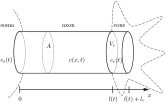
Figure 1: Schematic illustration of a growing axon.

In Figure 1, an idealized axon is shown. The one-dimensional $x$-axis is placed along the axon, which at time $t$ [s] has the length $l(t)$ [m]. The latter variable is one output of the model. The effective cross-sectional area of the axon through which tubulin is transported is assumed to be a constant denoted by $A$ [m²]. Another output of the model is the concentration of tubulin along the axon, which is assumed to vary with $x$ and $t$; i.e. $c=c(x,t)$ [mol$/$m³]. Tubulin is produced only in the cell body, the soma, which is placed to the left of $x=0$. We assume that the time-varying tubulin concentration in the soma $c_{\mathrm{s}}(t)$ is known. No tubulin is produced along the axon, but degradation occurs at the constant rate $g$ [1$/$s]. The tip of the axon, the growth cone, is located to the right of $x=l(t)$, and has the volume $V_{\mathrm{c}}$ [m³]. For simplicity, we introduce a characteristic length of the growth cone; $l_{\mathrm{c}}:=V_{\mathrm{c}}/A$ (it turns out that the final model only contains this ratio). The growth cone is considered to be a completely mixed compartment in which the unknown concentration of tubulin dimers is denoted by $c_{\mathrm{c}}(t)$. No production of tubulin occurs in the cone, but consumption occurs, partly because of degradation at the constant rate $g$ [1$/$s], partly because of the assembly of dimers to microtubules that elongates the axon at a constant rate $\tilde{r}_{\mathrm{g}}$ [1$/$s], i.e., $\tilde{r}_{\mathrm{g}}$ is the reaction rate of polymerization of guanosine triphosphate (GTP) bound tubulin dimers to microtubule bound guanosine diphosphate (GDP). As for the polymerization, we let $A_{\mathrm{g}}$ [m²] denote the constant effective area of growth and $\rho$ [mol$/$m³] the density of the assembled microtubules (the cytoskeleton). Finally, we assume that the assembled microtubules in the growth cone may disassemble at the constant rate $\tilde{s}_{\mathrm{g}}$ [$1/$s]. All biological and physical constants are assumed to be non-negative.

2.2 The conservation law of mass and constitutive assumptions

The conservation of mass of tubulin states that the rate of increase of mass in an arbitrary interval $(x_{1},x_{2})$ of the $x$-axis equals the mass flux (mol per unit time) in minus the flux out plus the production inside the interval:

$$\frac{\mathrm{d}{}}{\mathrm{d}{t}}\int\limits_{x_{1}}^{x_{2}}Ac(x,t)\,\mathrm{d}x=A\left(F|_{x=x_{1}}-F|_{x=x_{2}}\right)+\int\limits_{x_{1}}^{x_{2}}AS_{\!\mathrm{a}}\,\mathrm{d}x,$$ (1)

where $F$ [mol$/($m²s$)$] is the flux per unit area of tubulin and $S_{\!\mathrm{a}}$ [mol$/($m³s$)$] is a source/sink modelling local production/consumption in the axon. Since only degradation is taken into account, we have $S_{\!\mathrm{a}}=-gc$. Note that the flux $F$ is the product of the concentration $c$ and the velocity of tubulin $v$ [m$/$s]:

$$F=cv.$$ (2)

The conservation law (1) yields two dynamic equations. Letting the interval $(x_{1},x_{2})$ shrink to a point $x\in(0,l(t))$ one gets the PDE (assuming $c$ and $F$ are continuously differentiable functions):

$$\frac{\partial{c}}{\partial{t}}+\frac{\partial{F}}{\partial{x}}=-gc\quad\text{for}\quad 0<x<l(t).$$ (3)

This is one equation with two unknowns; $c$ and $F$ (or $v$). A constitutive assumption is needed. It is often assumed that the flux of tubulin $F$ is determined by active transport by motor proteins having the constant velocity $a$ [m$/$s] and diffusion of free tubulin according to Fick’s law [3, 4, 7, 8, 11, 12, 15, 22, 26, 27, 20]. The constitutive assumption relating the flux $F$ and the concentration $c$ is

$$F(c,c_{x})=ac-Dc_{x},$$ (4)

where $D$ [m${}^{2}/$s] is the diffusion coefficient and $c_{x}=\partial c/\partial x$. Substitution of (4) into PDE (3) gives the advection-diffusion-reaction equation

$$\frac{\partial{c}}{\partial{t}}+a\frac{\partial{c}}{\partial{x}}-D\frac{\partial^{2}c}{\partial x^{2}}=-gc\quad\text{for}\quad 0<x<l(t).$$ (5)

The conservation of mass (1) should also hold for the growth cone located in the interval $(x_{1},x_{2})=(l(t),l(t)+l_{\mathrm{c}})$. Over (the moving) right boundary $x=l(t)+l_{\mathrm{c}}$, there is no flux; however, there is over $x=l(t)$. To write down this flux from left to right, we introduce the following notation:

$$c^{-} :=c\big{(}l(t)^{-},t\big{)}=\lim_{\epsilon\searrow 0}c\big{(}l(t)-\epsilon,t\big{)},$$

which is the concentration just to the left of the boundary $x=l(t)$. Similarly, we use the notation $c_{x}^{-}$ and $v^{-}$. The boundary $x=l(t)$ moves with velocity $l^{\prime}(t)=\mathrm{d}{l}/\mathrm{d}{t}$ while the tubulin moves with the velocity $v^{-}$. If $v^{-}$ is higher than $l^{\prime}(t)$, then there is a net inflow of tubulin to the growth cone; otherwise, there is an outflow. Hence, it is the relative velocity of tubulin $v^{-}-l^{\prime}(t)$ that determines whether the net influx is positive or negative. Since the flux (amount per unit time) is the product of the net velocity, the concentration and the cross-sectional area, the net flux over $x=l(t)$ in the $x$-direction is

$$A\big{(}v^{-}-l^{\prime}(t)\big{)}c^{-}.$$ (6)

With the physical law (2) and the constitutive assumption for $F$ (4), the velocity of tubulin can be written

$$v(c,c_{x})=\frac{F(c,c_{x})}{c}=a-D\frac{c_{x}}{c}.$$

Substituting this into (6), we get the flux [mol$/$s] of tubulin over $x=l(t)$ (seen by an observer moving with the boundary):

$$A\big{(}ac^{-}-Dc_{x}^{-}-l^{\prime}(t)c^{-}\big{)}.$$ (7)

The conservation of the amount of free tubulin in the growth cone leads to the following ODE:

$$\begin{split}&\underbrace{\frac{\mathrm{d}{(V_{\mathrm{c}}c_{\mathrm{c}})}}{\mathrm{d}{t}}}_{\text{mass increase per unit time}}=\\ &=\underbrace{A\big{(}ac^{-}-Dc_{x}^{-}-l^{\prime}(t)c^{-}\big{)}}_{\text{flux in}}-\underbrace{gV_{\mathrm{c}}c_{\mathrm{c}}}_{\text{degradation}}-\underbrace{\tilde{r}_{\mathrm{g}}V_{\mathrm{c}}c_{\mathrm{c}}}_{\text{assembly}}+\underbrace{\tilde{s}_{\mathrm{g}}\rho A_{\mathrm{g}}\kappa l_{\mathrm{c}}}_{\text{disassembly}}.\end{split}$$ (8)

We assume that the degradation of free tubulin occurs at the same rate $g$ as in the entire axon. The two last terms describe mass per unit time of the assembly/disassembly (polymerization/deplymerization) of microtubules. The assembled mass per unit time is assumed to be proportional to the available amount of tubulin in the cone $V_{\mathrm{c}}c_{\mathrm{c}}(t)$ with the reaction rate $\tilde{r}_{\mathrm{g}}$ as the proportionality constant. The disassembly at the rate $\tilde{s}_{\mathrm{g}}$ is a process that reduces the growth rate, and is proportional to the already assembled microtubules, $\rho A_{\mathrm{g}}\kappa l_{\mathrm{c}}$, where $\kappa>0$ is a dimensionless constant such that $\kappa l_{\mathrm{c}}$ is the length of the assembled microtubles that may undergo disassembly. Experimental evidence that this term is independent of the free tubulin concentration has been provided by Walker et al. [28].

Before simplifying Equation (8), we note that it contains the two unknown functions $c_{\mathrm{c}}(t)$ and $l(t)$. A relation between these is needed. The conservation of the amount of assembled (polymerized) tubulin is the following, where the terms on the right-hand side have been explained above; see the two last terms of (8):

$$\underbrace{\frac{\mathrm{d}{(\rho A_{\mathrm{g}}l)}}{\mathrm{d}{t}}}_{\text{mass increase per unit time}}=\underbrace{\tilde{r}_{\mathrm{g}}V_{\mathrm{c}}c_{\mathrm{c}}(t)}_{\text{assembly}}-\underbrace{\tilde{s}_{\mathrm{g}}\rho A_{\mathrm{g}}\kappa l_{\mathrm{c}}}_{\text{disassembly}}.$$ (9)

Since the density $\rho$ and growth area $A_{\mathrm{g}}$ of assembled microtubules are assumed to be constants, we can divide Equation (9) by $\rho A_{\mathrm{g}}$ and obtain

$$\frac{\mathrm{d}{l}}{\mathrm{d}{t}}=\frac{\tilde{r}_{\mathrm{g}}V_{\mathrm{c}}}{\rho A_{\mathrm{g}}}c_{\mathrm{c}}(t)-\tilde{s}_{\mathrm{g}}\kappa l_{\mathrm{c}}.$$ (10)

If the concentration of tubulin is too low, this equation yields that the elongation is negative, which means that the axon shrinks. To compare with the notation in the model of McLean and Graham [12], who write the equation $l^{\prime}(t)=r_{\mathrm{g}}c_{\mathrm{c}}-s_{\mathrm{g}}$, we set

$$r_{\mathrm{g}}:=\frac{\tilde{r}_{\mathrm{g}}V_{\mathrm{c}}}{\rho A_{\mathrm{g}}}\quad\text{and}\quad s_{\mathrm{g}}:=\tilde{s}_{\mathrm{g}}\kappa l_{\mathrm{c}},$$

where $s_{\mathrm{g}}$ is easily interpreted as the maximum speed of shrinkage, which occurs when $c_{\mathrm{c}}=0$. The parameter $r_{\mathrm{g}}$ is a sort of rate coefficient for the polymerization; however, it has not the unit of a rate constant. It is the proportionality concentration between the resulting elongation speed due to the polymerization and $c_{\mathrm{c}}$ when there is now disassembly. We also define

$$c_{\infty}:=\frac{s_{\mathrm{g}}}{r_{\mathrm{g}}}=\frac{\tilde{s}_{\mathrm{g}}\rho A_{\mathrm{g}}\kappa l_{\mathrm{c}}}{\tilde{r}_{\mathrm{g}}V_{\mathrm{c}}}=\frac{\tilde{s}_{\mathrm{g}}\rho A_{\mathrm{g}}\kappa}{\tilde{r}_{\mathrm{g}}A},$$ (11)

which is the threshold concentration when $l^{\prime}(t)=0$, i.e. when there is no elongation, since the processes of assembly and disassembly are equally large. Therefore, $c_{\infty}$ is the steady-state concentration in the growth cone. Then (10) can be written

$$\frac{\mathrm{d}{l}}{\mathrm{d}{t}}=r_{\mathrm{g}}(c_{\mathrm{c}}(t)-c_{\infty}).$$ (12)

Thus, $r_{\mathrm{g}}$ is the proportionality constant between the elongation speed and the excess tubulin concentration in the growth cone above the steady-state level $c_{\infty}$.

We now simplify Equation (8) by dividing by $A$, use (11) to introduce $c_{\infty}$ and use (12) to express it without $l^{\prime}(t)$:

$$l_{\mathrm{c}}\frac{\mathrm{d}{c_{\mathrm{c}}}}{\mathrm{d}{t}}=ac^{-}-Dc_{x}^{-}-r_{\mathrm{g}}(c_{\mathrm{c}}-c_{\infty})c^{-}-gl_{\mathrm{c}}c_{\mathrm{c}}-\tilde{r}_{\mathrm{g}}l_{\mathrm{c}}c_{\mathrm{c}}+\tilde{r}_{\mathrm{g}}l_{\mathrm{c}}c_{\infty}.$$ (13)

2.3 Model equations with boundary and initial conditions

The three model equations are (5), (12) and (13), and the unknowns are $c(x,t)$, $c_{\mathrm{c}}(t)$ and $l(t)$. The physical/biological parameters that need to be specified are $a$, $D$, $g$, $l_{\mathrm{c}}$, $\tilde{r}_{\mathrm{g}}$, $r_{\mathrm{g}}$, $c_{\infty}$ and $c_{\mathrm{s}}(t)$. When diffusion is present ($D>0$) it is well known that the parabolic equation (5) has smooth solutions $c(x,t)$. Therefore, it is natural to impose boundary conditions requiring that the concentration is continuous at $x=0$ and $x=l$. In particular, this means that $c^{-}=c(l(t),t)=c_{\mathrm{c}}(t)$, which simplifies the right-hand side of (13). Initially, we assume that the neurite that becomes the axon has the length $l_{0}>0$ (which may be small) and that the given initial concentration distribution is $c_{0}(x)$ (the index denotes $t=0$). From a mathematical point of view, the function $c_{0}(x)$ can be chosen rather freely; however, a natural choice for a small neurite may be the soma concentration. The full model is the following:

$$\left\{\begin{aligned} &\frac{\partial{c}}{\partial{t}}+a\frac{\partial{c}}{\partial{x}}-D\frac{\partial^{2}c}{\partial x^{2}}=-gc,&\quad&0<x<l(t),\ t>0,\\ &\begin{split}&l_{\mathrm{c}}\frac{\mathrm{d}{c_{\mathrm{c}}}}{\mathrm{d}{t}}=(a-gl_{\mathrm{c}})c_{\mathrm{c}}-Dc_{x}^{-}\\ &\qquad-(r_{\mathrm{g}}c_{\mathrm{c}}+\tilde{r}_{\mathrm{g}}l_{\mathrm{c}})(c_{\mathrm{c}}-c_{\infty}),\end{split}&&t>0,\\ &\frac{\mathrm{d}{l}}{\mathrm{d}{t}}=r_{\mathrm{g}}(c_{\mathrm{c}}-c_{\infty}),&&t>0,\\ &c(0,t)=c_{\mathrm{s}}(t),&&t\geq 0,\\ &c\big{(}l(t),t\big{)}=c_{\mathrm{c}}(t),&&t>0,\\ &c(x,0)=c_{0}(x),&&0\leq x\leq l(0)=l_{0},\\ &c_{\mathrm{c}}(0)=c_{0}(l_{0}).&&\\ \end{aligned}\right.$$ (14)

Since we are interested in steady-state solutions in this work, we will mostly use a constant soma concentration.

3 Parameter values

The values of the model parameters are collected from the literature. The nominal values and possible intervals are given in Table 1. Here, we motivate our choices.

Table 1: Parameter values. In steady state, the nominal parameter values together with the constant soma concentration $c_{\mathrm{s}}=c_{\infty}$ imply $l_{\infty}=65.6$ mm (see Figure 6).

Parameter	Nominal value	Interval	Unit
$a$	$1$	$0.5$–$3$	$10^{-8}$ m$/$s
$D$	$10$	$1$–$25$	$10^{-12}$ m${}^{2}/$s
$g$	$5$	$1$–$200$	$10^{-7}$ s-1
$l_{\mathrm{c}}$	$4$	$0.1$–$1000$	$10^{-6}$ m
$r_{\mathrm{g}}$	$1.783$	—	$10^{-5}$ m${}^{4}/($mol s$)$
$\tilde{r}_{\mathrm{g}}$	0.053	—	s-1
$c_{\infty}$	$11.90$	—	$10^{-3}$ mol$/$m3
$c_{\mathrm{s}}$	—	$0$–$4c_{\infty}$	mol$/$m3

Galbraith et al. [4] present experimentally determined values for the transportation of tubulin in the giant squid axon. For the active transport, they obtained $a=93.9~{}\mu$m$/$h $\approx 2.3$ mm$/$day $\approx 2.66\cdot 10^{-8}$ m$/$s and the diffusion coefficient was about $D=8.59~{}\mu$m${}^{2}/$s $=8.59\cdot 10^{-12}$ m${}^{2}/$s. Reported active transport speeds for other animals are $a\approx$ 0.5–2 mm$/$day; see Galbraith and Gallant [3, Table 1] and Miller and Samuels [16, Table 1], and the references therein. Experiments with cultured neuronal cells by Keith [10] yielded the two different values $a=2.3$ mm$/$day and $0.31$ mm$/$day for the slow components a and b, respectively.

Salmon et al. [21] have measured the radial diffusion of tubulin in cytoplasm of eggs and embryos of the sea urchin Lytechinus variegatus and via the linear diffusion equation estimated the diffusion coefficient to $D=5.9\cdot 10^{-12}$ m${}^{2}/$s. Other experiments have resulted in diffusion coefficients of the same order, e.g., Pepperkok et al. [19] report values between $1.3\cdot 10^{-12}$ m${}^{2}/$s and $1.6\cdot 10^{-12}$ m${}^{2}/$s.

As for the tubulin degradation, Caplow et al. [1] report the half-times of 9.6 h for tubulin-GTP and 2.4 h for tubulin-GDP, which give the degradation rates $g=\ln 2/(9.6\cdot 3600)~{}\text{s}^{-1}\approx 2.0\cdot 10^{-5}~{}\text{s}^{-1}$ and $5\cdot 10^{-6}~{}\text{s}^{-1}$, respectively. Miller and Samuels [16, Table 1] report several published experimental results with half-times of 14–75 days, which correspond to $g$ between $1.1\cdot 10^{-7}~{}\text{s}^{-1}$ and $5.7\cdot 10^{-7}~{}\text{s}^{-1}$. It seems to be of interest to investigate the outputs of the model for a large interval of values of $g$.

As in the model by McLean and Graham [12], we condense all complicated building processes in the growth cone and assume that the axonal elongation can be described by Equation (12). Appropriate values should be found for the concentration-rate coefficient $r_{\mathrm{g}}$ and either the steady-state concentration $c_{\infty}$ or the maximum speed of shrinkage $s_{\mathrm{g}}=r_{\mathrm{g}}c_{\infty}$. It is sometimes argued that the speed of axonal elongation from the soma is similar, or equal, to the speed of growth $\upsilon_{+}$ of the plus-end assembly of individual microtubules [6, 17]. Published experiments have shown that the growth speeds $\upsilon_{+}$ and $\upsilon_{-}$ for the plus and minus end, respectively, of an independent microtubule depend on the surrounding free tubulin concentration $c_{\mathrm{c}}$ according to the affine relationships

$$\upsilon_{+} =\alpha_{+}c_{\mathrm{c}}-\beta_{+},$$ (15)

$$\upsilon_{-} =\alpha_{-}c_{\mathrm{c}}-\beta_{-},$$ (16)

for positive constants $\alpha_{+}>\alpha_{-}$, $\beta_{+}$ and $\beta_{-}$ [17, 28]. The dynamic growth of a microtubule consists of phases of growth alternated by rapid shortening due to depolymerization. The shortening phase has a speed that seems to be independent of concentration [28]. Furthermore, both the growth and shortening phases contain periods of pauses.

Mitchison and Kirschner [17] report the experimental values

$$\text{$\alpha_{+}=0.135~{}$m$/(\text{M\,min})=2.25\cdot 10^{-6}~{}\text{m}^{4}/(\text{mol\,s})$},$$

$$\text{$\alpha_{-}=0.042~{}$m$/(\text{M\,min})=0.70\cdot 10^{-6}~{}\text{m}^{4}/(\text{mol\,s})$},$$

and $\beta_{+}$ and $\beta_{-}$ small (near zero). For the same tubulin preparation, the steady-state concentration, when the average elongation/shortening of many microtubules is zero, was $14~{}\mu$M $=14\cdot 10^{-3}$ mol$/$m³, which together with the obtained constants $\alpha_{\pm}$ means that both ends are growing in steady-state ($\upsilon_{+},\upsilon_{-}>0$). Hence, there are other processes, such as the rapid shortening, that make the average growing speed be zero. Mitchison and Kirschner [17] argue that in steady-state the majority of the microtubules that grow slowly is balanced by the minority shrinking rapidly.

Graham et al. [6] refer to the value $\alpha_{+}=2.25\cdot 10^{-6}~{}\text{m}^{4}/(\text{mol\,s})$ of Mitchison and Kirschner [17] when they choose $r_{\mathrm{g}}=2.78\cdot 10^{-6}~{}\text{m}^{4}/(\text{mol\,s})$ in Equation (12) for their model, which is the one by McLean and Graham [12]. Then they choose $c_{\infty}=10~{}\mu$M as the common order of concentration.

Walker et al. [28] presented further detailed measurements of the individual microtubules in porcine brain tubulin and obtained the following values for (15)–(16):

$$\text{$\alpha_{+}=0.33~{}$m$/(\text{M\,min})=5.5\cdot 10^{-6}~{}\text{m}^{4}/(\text{mol\,s})$},$$ (17)

$$\text{$\beta_{+}=1.59\cdot 10^{-6}$~{}m$/\text{min}=2.65\cdot 10^{-8}$~{}m$/\text{s}$},$$ (18)

$$\text{$\alpha_{-}=0.15~{}$m$/(\text{M\,min})=2.5\cdot 10^{-6}~{}\text{m}^{4}/(\text{mol\,s})$},$$

$$\text{$\beta_{-}=0.85\cdot 10^{-6}$~{}m$/\text{min}=1.42\cdot 10^{-8}$~{}m$/\text{s}$}.$$

It is interesting to note that, with these values, the two lines (15)–(16) intersect at the concentration $\approx 5~{}\mu$M, which is also the concentration at which $\upsilon_{+}\approx\upsilon_{-}\approx 0$. The rapid shortening speeds were measured to $27~{}\mu$m$/$min and $34~{}\mu$m$/$min for the plus and minus end, respectively, independently of the surrounding tubulin concentration. We note that Janulevicius et al. [9] use the values (17), (18) and $27~{}\mu$m$/$min (from Walker et al. [28]) for their model of dynamic instability. The model consists of a growth phase with the velocity given by (15), a shrinkage phase with constant shrinkage speed $27~{}\mu$m$/$min, and two affine relationships between the frequencies of rescue and catastrophe as functions of the tubulin concentration, also with coefficients from the measurements of Walker et al. [28]. These frequencies are then used in a probability density function of an exponential distribution of waiting times between different possible events.

To obtain the combined average effect of elongation and rapid shortening of the plus and minus ends, Walker et al. [28] took into account the average times for the different phases and obtained the affine relationships shown in their Figure 9 for the plus and minus end, respectively. The sum of these two functions gives an affine relationship for an average microtubule and shows that the steady-state concentration is $10.9~{}\mu$M tubulin. Their corresponding experimentally measured value was in the range 6.9–7.5 $\mu$M. For the assembly of tubulin dimers in the growth cone of an axon, we are interested in only the average growth of the plus-ends of microtubules. This velocity as a function of tubulin concentration is given by a straight line in [28, Figure 9]. We collect the following two points on the line: $(c_{1},\upsilon_{1})=(14.43~{}\mu\text{M},73.42\text{~{}dimers}/\text{s})$ and $(c_{2},\upsilon_{2})=(7.99~{}\mu\text{M},-113.04\text{~{}dimers}/\text{s})$. To express the velocity in SI units, we assume that there are 1625 dimers per $\mu$m of microtubule as Janulevicius et al. [9] do, i.e. a dimer has the length $6.1538\cdot 10^{-10}$ m. This value agrees well with other values in [28] for which elongation speeds are expressed in both m$/$s and dimers$/$s. In SI units, the two collected points are $(c_{1},\upsilon_{1})=(0.01443~{}\text{mol}/\text{m}^{3},4.518\cdot 10^{-8}\text{~{}m}/\text{s})$ and $(c_{2},\upsilon_{2})=(0.00799~{}\text{mol}/\text{m}^{3},-6.956\cdot 10^{-8}\text{~{}m}/\text{s})$ from which we obtain

$$r_{\mathrm{g}} =\frac{\upsilon_{1}-\upsilon_{2}}{c_{1}-c_{2}}=1.783\cdot 10^{-5}~{}\text{m}^{4}/(\text{mol\,s}),$$ (19)

$$s_{\mathrm{g}} =-(\upsilon_{1}-r_{\mathrm{g}}c_{1})=2.121\cdot 10^{-7}~{}\text{m}/\text{s},$$ (20)

and hence $c_{\infty}=s_{\mathrm{g}}/r_{\mathrm{g}}=11.90\cdot 10^{-3}$ mol$/$m³.

Janulevicius et al. [9] estimate from the data of Tanaka and Sabry [24] that the volume of a growth cone $V_{\mathrm{c}}$ lies in the range 1–200 $\mu$m³. Approximating the growth cone by a sphere, this has then a radius in the range 0.62–3.6 $\mu$m. We expect our parameter $l_{\mathrm{c}}$ to be of this order.

The remaining parameter in the dynamic model (14) is the polymerization reaction rate constant $\tilde{r}_{\mathrm{g}}$; see (9). This constant appears only in the factor $(r_{\mathrm{g}}c_{\mathrm{c}}+\tilde{r}_{\mathrm{g}}l_{\mathrm{c}})$ in the equation for the cone concentration in the model(14). To define a nominal value we assume that $\tilde{r}_{\mathrm{g}}l_{\mathrm{c}}$ is of the same order as $r_{\mathrm{g}}c_{\mathrm{c}}$. With $l_{\mathrm{c}}=4$ $\mu$m, $c_{\mathrm{c}}=c_{\infty}=11.9\cdot 10^{-3}$ mol$/$m³ and $r_{\mathrm{g}}$ given by (19), we get the nominal value $\tilde{r}_{\mathrm{g}}=0.053$ $s^{-1}$.

4 All steady-state solutions and their properties

It is interesting to investigate the possible steady-state solutions of a dynamic model. If the given soma concentration $c_{\mathrm{s}}$ is constant and all variables $c$, $l$, $c_{\mathrm{c}}$ of the model equations (14) are assumed to be independent of time, then we denote the unknown constant axon length by $l_{\infty}$, and note that $c_{\mathrm{c}}=c_{\infty}$ holds by the ODE for $l^{\prime}(t)$. Then the model equations (14) yield the following linear boundary-value problem for the unknown function $c=c(x)$ and the constant $l_{\infty}>0$:

$$\left\{\begin{aligned} &D\frac{\mathrm{d}^{2}c}{\mathrm{d}x^{2}}-a\frac{\mathrm{d}{c}}{\mathrm{d}{x}}-gc=0,&\quad&0<x<l_{\infty},\\ &Dc^{\prime}(l_{\infty})=(a-gl_{\mathrm{c}})c_{\infty},&&\\ &c(l_{\infty})=c_{\infty},&&\\ &c(0)=c_{\mathrm{s}}.&&\\ \end{aligned}\right.$$ (21)

Note that the two parameters $r_{\mathrm{g}}$ and $\tilde{r}_{\mathrm{g}}$ are not present in (21), which means that they only influence dynamic solutions, not steady-state solutions.

4.1 The case $a>0$, $D>0$ and $g>0$

The general solution of the ODE in (21) is

$$c(x)=k_{+}\mathrm{e}^{\lambda_{+}x}+k_{-}\mathrm{e}^{\lambda_{-}x},$$

$$\text{where}\quad\lambda_{\pm}:=\frac{a\pm R}{2D}\quad\text{and}\quad R:=\sqrt{{a^{2}}+4gD},$$

and where $k_{\pm}$ are two constants. We note that

$$\lambda_{-}<0<\lambda_{+},\quad\lambda_{+}-\lambda_{-}=\frac{R}{D},\quad\lambda_{+}+\lambda_{-}=\frac{a}{D},$$

which we will use in the calculations below. The three boundary conditions in (21) give

$$\left\{\begin{aligned} &Dk_{+}\lambda_{+}\mathrm{e}^{\lambda_{+}l_{\infty}}&&+Dk_{-}\lambda_{-}\mathrm{e}^{\lambda_{-}l_{\infty}}&&=(a-gl_{\mathrm{c}})c_{\infty}\\ &k_{+}\mathrm{e}^{\lambda_{+}l_{\infty}}&&+k_{-}\mathrm{e}^{\lambda_{-}l_{\infty}}&&=c_{\infty}\\ &k_{+}&&+k_{-}&&=c_{\mathrm{s}}.\end{aligned}\right.$$ (22)

From the two upper equations of (22) we can express $k_{\pm}$ in terms of $l_{\infty}$, for example, by using Cramer’s rule. The coefficient determinant is

$$\Delta:=D(\lambda_{+}-\lambda_{-})\mathrm{e}^{\lambda_{+}l_{\infty}}\mathrm{e}^{\lambda_{-}l_{\infty}}=R\mathrm{e}^{al_{\infty}/D}.$$

Then we get

$$k_{+} =\frac{1}{\Delta}\begin{vmatrix}(a-gl_{\mathrm{c}})c_{\infty}&D\lambda_{-}\mathrm{e}^{\lambda_{-}l_{\infty}}\\ c_{\infty}&\mathrm{e}^{\lambda_{-}l_{\infty}}\end{vmatrix}=\frac{c_{\infty}\mathrm{e}^{\lambda_{-}l_{\infty}}}{R\mathrm{e}^{al_{\infty}/D}}(a-gl_{\mathrm{c}}-D\lambda_{-})$$

$$=\frac{c_{\infty}\mathrm{e}^{-\lambda_{+}l_{\infty}}}{R}\left(\frac{R+a}{2}-gl_{\mathrm{c}}\right)$$

and analogously

$$k_{-} =\frac{1}{\Delta}\begin{vmatrix}D\lambda_{+}\mathrm{e}^{\lambda_{+}l_{\infty}}&(a-gl_{\mathrm{c}})c_{\infty}\\ \mathrm{e}^{\lambda_{+}l_{\infty}}&c_{\infty}\end{vmatrix}=\frac{c_{\infty}\mathrm{e}^{\lambda_{+}l_{\infty}}}{R\mathrm{e}^{al_{\infty}/D}}(D\lambda_{+}-a+gl_{\mathrm{c}})$$

$$=\frac{c_{\infty}\mathrm{e}^{-\lambda_{-}l_{\infty}}}{R}\left(\frac{R-a}{2}+gl_{\mathrm{c}}\right).$$

Now the third equation of (22) can be written with only one unknown, $l_{\infty}$:

$$\frac{1}{R}\left[{\mathrm{e}^{-\lambda_{+}l_{\infty}}}\left(\frac{R+a}{2}-gl_{\mathrm{c}}\right)+{\mathrm{e}^{-\lambda_{-}l_{\infty}}}\left(\frac{R-a}{2}+gl_{\mathrm{c}}\right)\right]=\frac{c_{\mathrm{s}}}{c_{\infty}}.$$ (23)

We can write this equation $f(l_{\infty})={c_{\mathrm{s}}}/c_{\infty}$, where

$$f(z) :=\frac{1}{R}\left[{\mathrm{e}^{-\lambda_{+}z}}\left(\frac{R+a}{2}-gl_{\mathrm{c}}\right)+{\mathrm{e}^{-\lambda_{-}z}}\left(\frac{R-a}{2}+gl_{\mathrm{c}}\right)\right],$$ (24)

$$f^{\prime}(z) =\frac{1}{R}\left[-\lambda_{+}{\mathrm{e}^{-\lambda_{+}z}}\left(\frac{R+a}{2}-gl_{\mathrm{c}}\right)-\lambda_{-}{\mathrm{e}^{-\lambda_{-}z}}\left(\frac{R-a}{2}+gl_{\mathrm{c}}\right)\right].$$ (25)

Note that $f(0)=1$, which via (23) corresponds to $c_{\infty}=c_{\mathrm{s}}$. The second terms within the squared brackets of both (24) and (25) are positive (since $\lambda_{-}<0$ and $R>a$). This means that both $f(z),f^{\prime}(z)\rightarrow\infty$ (exponentially fast) as $z\rightarrow\infty$. A graph of the function $f(z)$ given by (24) is shown in Figure 2.

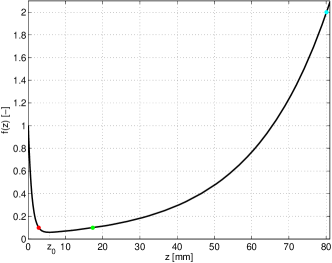
Figure 2: A graph of the function $f(z)$ given by (24) for the nominal values of Table 1, which means that Case I of Theorem 4.1 is valid. Note that the steady-state length $l_{\infty}$ is obtained from the equation $f(l_{\infty})=c_{\mathrm{s}}/c_{\mathrm{c}}$. For a given value of the ratio $c_{\mathrm{s}}/c_{\mathrm{c}}$ on the $f(z)$-axis, one can easily read off the number of steady-state solutions and approximately the corresponding length(s) $l_{\infty}$ on the $z$-axis. For example, when $c_{\mathrm{s}}/c_{\mathrm{c}}=0.1$, there are two steady-state solutions corresponding to the red and green dots; see Figure 3. As $c_{\mathrm{s}}/c_{\mathrm{c}}=2$, there is a unique steady-state solution (magenta dot); see Figure 4.

We now investigate two main cases.

Assume first that $gl_{\mathrm{c}}<(R+a)/2$ holds. Then and only then the first term (within the squared brackets) of (25) is negative, which is equivalent to the fact that the equation $f^{\prime}(z_{0})=0$ has the unique solution

$$z_{0} =\frac{D}{R}\log\frac{(R+a)(R+a-2gl_{\mathrm{c}})}{(R-a)(R-a+2gl_{\mathrm{c}})}.$$ (26)

Since $f^{\prime}(z)\rightarrow\infty$ as $z\rightarrow-\infty$, we can conclude that $f(z)$ is a unimodal function with $z_{0}$ as its unique global minimum point; see Figure 2. The nominal parameter values give

$$gl_{\mathrm{c}}=2\cdot 10^{-12}\text{~{}m$/$s}~{}<1\cdot 10^{-8}\text{~{}m$/$s~{}}=a.$$

Then one can compute $R=1.10\cdot 10^{-8}\text{~{}m$/$s}$ and

$$z_{0} =5.64\text{~{}mm},\quad f(z_{0})=0.060.$$

The following equivalence is valid for the number $z_{0}$ given by (26):

$$z_{0}>0 \quad\Longleftrightarrow\quad\frac{(R+a)(R+a-2gl_{\mathrm{c}})}{(R-a)(R-a+2gl_{\mathrm{c}})}>1$$

$$\quad\Longleftrightarrow\quad gl_{\mathrm{c}}<a.$$

Hence, for $gl_{\mathrm{c}}<a<(a+R)/2$ we can conclude that $f(z)$ is decreasing for $0<z\leq z_{0}$ and increasing for $z\geq z_{0}$. In particular, $f(z_{0})<f(0)=1$ holds. Furthermore, since $gl_{\mathrm{c}}<a<(a+R)/2$, it is clear that $f(z)>0$ for all $z$, in particular, $f(z_{0})>0$. Hence, we may have zero, one or two steady-state solutions depending on the parameter values. In the subcase $a\leq gl_{\mathrm{c}}<(R+a)/2\Leftrightarrow z_{0}\leq 0$, we conclude that $f(z)$ is increasing for $z\geq 0$, which implies that there exists a unique solution $l_{\infty}>0$ of (23) if and only if $f(0)=1<c_{\mathrm{s}}/c_{\infty}$ holds.

Assume now that $gl_{\mathrm{c}}\geq(R+a)/2$ holds. Then the first term of (25) is also positive, hence $f^{\prime}(z)>0$ for all $z$, which implies that (23) has a unique solution $l_{\infty}>0$ if and only if $f(0)=1<c_{\mathrm{s}}/c_{\infty}$ holds. We conclude the cases in the following theorem.

Theorem 4.1.

Assume that $a>0$, $D>0$, $g>0$ hold. Then the following cases may occur:

• $gl_{\mathrm{c}}<a$: There exists a $z_{0}>0$ given by (26). There are four subcases:

  • $c_{\mathrm{s}}/c_{\infty}<f(z_{0})<1$: No steady-state solution exists.

  • $c_{\mathrm{s}}/c_{\infty}=f(z_{0})$: There exists a unique steady-state solution of (21) with $l_{\infty}=z_{0}$ and $c(x)$ given by the decreasing function

    $$c(x)=\frac{c_{\infty}}{R}\left[\left(\frac{R+a}{2}-gl_{\mathrm{c}}\right)\mathrm{e}^{\lambda_{+}(x-l_{\infty})}\right.\\ \qquad\qquad\left.+\left(\frac{R-a}{2}+gl_{\mathrm{c}}\right)\mathrm{e}^{\lambda_{-}(x-l_{\infty})}\right],\quad 0\leq x\leq l_{\infty}.$$ (27)

  • $f(z_{0})<c_{\mathrm{s}}/c_{\infty}<1$: There exist two steady-state solutions. The axon lengths $l_{\infty 1}$ and $l_{\infty 2}$ satisfy $0<l_{\infty 1}<z_{0}<l_{\infty 2}$ and the corresponding concentration distributions $c_{1}(x)$ and $c_{2}(x)$ are given by (27). The function $c_{1}(x)$ is increasing for $0\leq x\leq l_{\infty 1}$ and $c_{2}(x)$ is decreasing for $0\leq x\leq l_{\infty 2}-z_{0}$ and increasing for $l_{\infty 2}-z_{0}\leq x\leq l_{\infty}$.

  • $c_{\mathrm{s}}/c_{\infty}\geq 1$: There exists a unique steady-state solution of (21) with $l_{\infty}>z_{0}$, and $c(x)$ given by (27) is decreasing for $0<x\leq l_{\infty}-z_{0}$ and increasing for $l_{\infty}-z_{0}\leq x\leq l_{\infty}$.

• $gl_{\mathrm{c}}\geq a$: If and only if $c_{\mathrm{s}}>c_{\infty}$ holds, there exists a unique solution $l_{\infty}>0$ of (23) and a unique steady-state solution of (21) given by (27), which is a decreasing function.

Proof.

What remains to be proved are the monotonicity properties of $c(x)$ in the different cases. Differentiation of (27) gives

$$c^{\prime}(x)=\frac{c_{\infty}}{R}\left[\left(\frac{R+a}{2}-gl_{\mathrm{c}}\right)\lambda_{+}\mathrm{e}^{\lambda_{+}(x-l_{\infty})}\right.\\ \qquad\qquad\left.+\left(\frac{R-a}{2}+gl_{\mathrm{c}}\right)\lambda_{-}\mathrm{e}^{\lambda_{-}(x-l_{\infty})}\right],\quad 0\leq x\leq l_{\infty}.$$ (28)

We first note that, within the squared brackets, the second term is negative, since $\lambda_{-}<0$. If $gl_{\mathrm{c}}<(R+a)/2$, then the equation $c^{\prime}(x_{0})=0$ has the unique solution

$$x_{0} =l_{\infty}-\frac{D}{R}\log\frac{(R+a)(R+a-2gl_{\mathrm{c}})}{(R-a)(R-a+2gl_{\mathrm{c}})}=l_{\infty}-z_{0}.$$ (29)

Furthermore, $c^{\prime}(x)\lessgtr 0$ for $x\lessgtr x_{0}$. Note that this covers Case I, since $gl_{\mathrm{c}}<a<(R+a)/2$. If $a\leq gl_{\mathrm{c}}<(R+a)/2$ holds, then $z_{0}\leq 0$, so that $x_{0}\geq l_{\infty}$. Hence $c(x)$ is decreasing for $0\leq x\leq l_{\infty}$. The remaining case is $gl_{\mathrm{c}}\geq(R+a)/2$. Then the first term of (28) (within the squared brackets) is negative, so that $c^{\prime}(x)<0$ holds. ∎

With the non-zero values of the parameters given in Table 1, the different types of steady-state solutions are given by Theorem 4.1. We now demonstrate and comment on the different cases of Theorem 4.1 by assigning $c_{\mathrm{s}}$ different values, rather we let the ratio $c_{\mathrm{s}}/c_{\infty}$ take different values. For the other parameters, we use the nominal values given in 1. Note how the graph in Figure 2 of the auxiliary function $f(z)$ visualizes the different subcases of Case I, since given a value on the ratio $c_{\mathrm{s}}/c_{\infty}$ on the vertical axis, one can read off the corresponding steady-state length(s) $l_{\infty}$ on the horizontal axis.

Case I.i

If $c_{\mathrm{s}}/c_{\infty}<f(z_{0})=0.060$, then there exists no steady-state solution with $l_{\infty}>0$. As can be seen in Figure 2, there exists no solution of the equation $f(z)=c_{\mathrm{s}}/c_{\infty}$ for values of $c_{\mathrm{s}}/c_{\infty}$ that lie below the minimum function value $f(z_{0})$.

The biological interpretation is that when the soma concentration satisfies $c_{\mathrm{s}}<c_{\infty}f(z_{0})=7.12\cdot 10^{-4}$ mol$/$m³, it is so small that no growth can occur. If the soma concentration was larger earlier so that the axon has reached a certain length and $cs$ drops to a value below $7.12\cdot 10^{-4}$ mol$/$m³, then the dynamic equation for the axon length in (14) implies that $l^{\prime}(t)<0$, i.e., the axon shrinks.

Case I.ii

This is a theoretical exceptional case with $c_{\mathrm{s}}/c_{\infty}=f(z_{0})=0.060$, which means that the only solution is the minimum point $z_{0}$ of $f$; hence the steady state length is the small number $l_{\infty}=z_{0}=5.64\text{~{}mm}$. The concentration distribution along the axon $c(x)$ is similar to the graph $c_{1}(x)$ shown in Figure 3.

The biological interpretation is that $c_{\mathrm{s}}=c_{\infty}f(z_{0})=7.12\cdot 10^{-4}$ mol$/$m³ is the smallest possible soma concentration that can result in a stationary axon; however, its length is small.

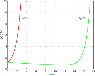
Figure 3: The two possible steady-state solutions in Case I.iii with the soma concentration $c_{\mathrm{s}}=1.19\cdot 10^{-3}$ mol$/$m³, which is lower than the cone concentration $c_{\infty}=11.9\cdot 10^{-3}$ mol$/$m³. Compare with the coloured dots in Figure 2.

Case I.iii

In this case $c_{\mathrm{s}}$ satisfies $f(z_{0})=0.060<c_{\mathrm{s}}/c_{\infty}<1$. One can see in Figure 2 that the equation $f(z)=c_{\mathrm{s}}/c_{\infty}$ then has two solutions; one is the small number $l_{\infty 1}<z_{0}$ and the other $l_{\infty 2}>z_{0}$. As an example, let $c_{\mathrm{s}}/c_{\infty}=0.1$, which means $c_{\mathrm{s}}=1.19\cdot 10^{-3}$ mol$/$m³. Then Equation (23) can be solved numerically to give $l_{\infty 1}=2.82$ mm and $l_{\infty 2}=17.3$ mm. The corresponding two concentration distributions along the axon are shown in Figure 3. In accordance with Theorem 4.1, $c_{2}(x)$ has a minimum point at $x=l_{\infty 2}-z_{0}=11.7$ mm.

The biological interpretation is that when the soma concentration $c_{\mathrm{s}}$ is smaller than $c_{\infty}$, then there are in fact two possible increasing concentration distributions along the axon (hence two possible $l_{\infty}$), for which the flux of positive active transport and negative diffusive transport is balanced by the degradation along the axon.

Case I.iv

In this case $c_{\mathrm{s}}>c_{\infty}$, holds and there is a unique steady-state solution. For example, $c_{\mathrm{s}}=2c_{\infty}=23.8\cdot 10^{-3}$ mol$/$m³ implies that $l_{\infty}=80.1$ mm and the concentration profile is shown in Figure 4.

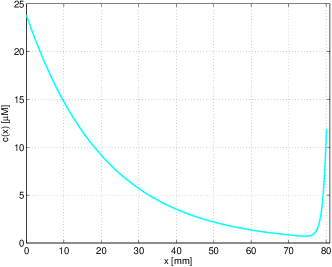
Figure 4: The Case I.iv with the soma concentration $c_{\mathrm{s}}=2c_{\infty}=23.8\cdot 10^{-3}$ mol$/$m³. Compare with the cyan dot in Figure 2.

The biological interpretation is that this is the normal case with a larger soma concentration than growth cone concentration. Note the non-monotone concentration $c(x)$ along the axon and that the concentration is lower than the growth cone concentration $c_{\infty}$ along most of the axon length (the interval between $x\approx 30$ mm and $x=l_{\infty}=80.1$ mm). The curve $c_{2}(x)$ in Figure 3 also has the same principle non-monotone form. The explanation for this non-monotone concentration profile $c(x)$ is that this very form is precisely such that all the following effects are precisely balanced: active transport, diffusion, degradation along the axon and in the growth cone, assembly and disassembly of tubulin dimers. All these effects are combined and it is therefore difficult to look at one or two separately in order to get an intuitive feeling for the form of $c(x)$. However, we discuss this further in Section 7.

Case II

In this case, the active transport coefficient satisfies $a<gl_{\mathrm{c}}=2\cdot 10^{-12}\text{~{}m$/$s}$. Such small values of $a$ yield, from a biological points of view, indistinguishable results from the case with $a=0$, which is is dealt with in the next subsection.

4.2 The case $a=0$, $D>0$ and $g>0$

This case with no advective transport is a special case of the one above with $R=2\sqrt{gD}$ and $\lambda_{\pm}=\pm\sqrt{g/D}$. It is easy to conclude that $z_{0}<0$. We are then in Case II of Theorem 4.1.

Theorem 4.2.

Assume that $a=0$, $D>0$ and $g>0$ hold. If and only if $c_{\mathrm{s}}>c_{\infty}$ holds there exists a unique solution $l_{\infty}>0$ of (23) and a unique steady-state solution of (21) given by

$$c(x)=\frac{c_{\infty}}{2}\left[\left(1-l_{\mathrm{c}}\sqrt{\frac{g}{D}}\right)\mathrm{e}^{(x-l_{\infty})\sqrt{\frac{g}{D}}}\right.\\ \qquad\qquad\left.+\left(1+l_{\mathrm{c}}\sqrt{\frac{g}{D}}\right)\mathrm{e}^{-(x-l_{\infty})\sqrt{\frac{g}{D}}}\right],\quad 0\leq x\leq l_{\infty},$$ (30)

which is a decreasing function.

In this case the only transport of tubulin from the soma to the growth cone is diffusion, wherefore a decreasing concentration distribution $c(x)$ is the only possibility (diffusion occurs from higher to lower concentrations). As an example, we choose $c_{\mathrm{s}}=4c_{\infty}=47.6\cdot 10^{-3}$ mol$/$m³, which yields the plots of Figure 5. The upper plot shows the auxiliary function $f(z)$, which is now increasing. As is shown by the magenta dot; despite a soma concentration $c_{\mathrm{s}}$ four times higher than $c_{\infty}$, the steady-state length is only $l_{\infty}=9.22$ mm. The corresponding concentration profile $c(x)$ given by (30) is shown in the lower plot of Figure 5.

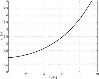
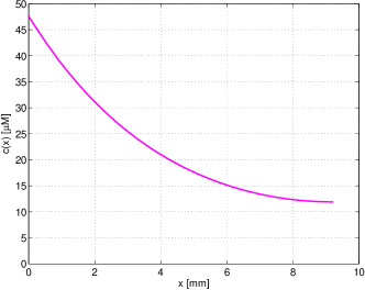
Figure 5: The case when $a=0$ (Theorem 4.2 or Case II of Theorem 4.1) with the ratio $c_{\mathrm{s}}/c_{\infty}=4$. Since the only transportation of tubulin occurs with diffusion, the steady-state length is much shorter than when active transport also is present ($a>0$).

4.3 The case $a>0$, $D>0$ and $g=0$

In this case we have $R=a$, $\lambda_{+}=a/D$ and $\lambda_{-}=0$. Then (23) is reduced to

$$a\mathrm{e}^{-al_{\infty}/D}=\frac{Rc_{\mathrm{s}}}{c_{\infty}}\quad\Longleftrightarrow\quad l_{\infty}=\frac{D}{a}\log\frac{c_{\infty}}{c_{\mathrm{s}}}.$$

Theorem 4.3.

Assume that $a>0$, $D>0$ and $g=0$. If and only if $c_{\mathrm{s}}<c_{\infty}$ holds there exists a unique solution $l_{\infty}>0$ of (23) and a unique steady-state solution of (21) given by

$$c(x)={c_{\infty}}\mathrm{e}^{(x-l_{\infty})a/D}=c_{\mathrm{s}}\mathrm{e}^{xa/D},\quad 0<x\leq l_{\infty}=\frac{D}{a}\log\frac{c_{\infty}}{c_{\mathrm{s}}}.$$

Since there is no degradation of tubulin, the total flux is zero at every point of the $x$-axis. This means that the active transport in the direction of increasing $x$-values is precisely balanced by diffusion in the opposite direction, which is possible if and only if $c(x)$ is increasing.

4.4 The case $D>0$ and $a=g=0$

In this case, the solution of the ODE in (21) is the affine function $c(x)=k_{1}x+k_{2}$, where $k_{1}$ and $k_{2}$ are constants to be determined by the boundary conditions of (21). One finds that for any value of $l_{\infty}>0$ the only possible solution is

$$c(x)=c_{\mathrm{s}}=c_{\infty},\quad 0<x\leq l_{\infty}.$$ (31)

Hence, there is neither any active ($a=0$) nor any diffusive transport, since the concentration is the same along the axon; the diffusive flux is $-Dc_{x}=-D\cdot 0=0$. Since there is no degradation, this case has probably no biological interest.

4.5 The cases with $D=0$

If there is no diffusion present, but $a>0$ and $g>0$, then the first boundary condition in (21) requires that $a=gl_{\mathrm{c}}$ holds, which one cannot expect to be fulfilled. However, if $a=gl_{\mathrm{c}}$ holds, then the steady-state solution satisfying the boundary conditions is

$$c(x)={c_{\infty}}\mathrm{e}^{(l_{\infty}-x)/l_{\mathrm{c}}}=c_{\mathrm{s}}\mathrm{e}^{-x/l_{\mathrm{c}}},\quad 0<x\leq l_{\infty}=l_{\mathrm{c}}\log\frac{c_{\mathrm{s}}}{c_{\infty}}.$$

Hence, $l_{\infty}>0$ if and only if $c_{\mathrm{s}}>c_{\infty}$, and then the concentration is decreasing along the axon.

In fact, when diffusion is not present, the extra assumption of a continuous concentration distribution is unnatural. When active transport is the only movement of a substance, then all waves, including discontinuities, in the concentration profile are transported with the velocity $a$. In fact, the PDE of (14) is hyperbolic and solutions of such may contain discontinuities travelling with the speed $a$ during dynamic situations. When there is no diffusion that can smooth out sharp gradients, one cannot exclude the case $c^{-}\neq c_{\mathrm{c}}$. Removing the continuity assumption, Equation (13) should be used for the dynamics of the cone concentration $c_{\mathrm{c}}$ instead of the second equation of (14) where the assumption $c^{-}=c_{\mathrm{c}}$ have been used. Then the boundary condition at $x=l(t)$ in (21) should be replaced by $Dc_{x}^{-}=ac^{-}-gl_{\mathrm{c}}c_{\mathrm{c}}$. Hence, when $D=0$ we have $ac^{-}=gl_{\mathrm{c}}c_{\mathrm{c}}$. This is a much more flexible condition that is fulfilled for all biologically possible parameter values. The steady-state problem is then reduced to

$$\left\{\begin{aligned} &-a\frac{\mathrm{d}{c}}{\mathrm{d}{x}}-gc=0,&\quad&0<x<l_{\infty},\\ &ac^{-}=gl_{\mathrm{c}}c_{\infty},&&\\ &c(0)=c_{\mathrm{s}}.&&\\ \end{aligned}\right.$$ (32)

Assume that $a>0$ and $g>0$. We first note that since any discontinuity in the interval $(0,l(t))$ has the positive speed $a$, there exists no stationary discontinuity. The only possible discontinuity in steady state is at $x=l_{\infty}$. Straightforward calculations give the following theorem.

Theorem 4.4.

Assume that $D=0$, $a>0$ and $g>0$ and consider the axonal-growth problem without the assumption that the concentration $c(x,t)$ is a continuous function, i.e., problem (14) with the ODE for $c_{\mathrm{c}}$ replaced by (13). If and only if $c_{\mathrm{s}}>c_{\infty}gl_{\mathrm{c}}/a$ holds there exists a unique steady-state solution of (32) given by

$$c(x)=c_{\mathrm{s}}\mathrm{e}^{-gx/a},\quad\text{and}\quad l_{\infty}=\frac{a}{g}\log\frac{ac_{\mathrm{s}}}{gl_{\mathrm{c}}c_{\infty}}.$$ (33)

Note that $c(l_{\infty})=c_{\mathrm{s}}\mathrm{e}^{-gl_{\infty}/a}=gl_{\mathrm{c}}c_{\infty}/a\neq c_{\infty}$, unless $a=gl_{\mathrm{c}}$ holds, which is the special case above when the solution is continuous. The cases when also either $a=0$ or $g=0$ are trivial and biologically uninteresting.

5 The steady-state solutions’ dependence on each parameter

Given the nominal parameter values of a steady-state solution (see Table 1), we shall now investigate the sensitivity of the steady-state solutions with respect to each parameter.

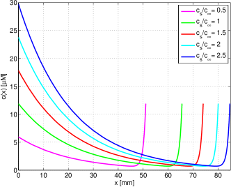
Figure 6: Concentration profiles for varying $c_{\mathrm{s}}$. Recall that $c_{\infty}=11.9~{}\mu$M. The magenta graph ($c_{\mathrm{s}}/c_{\infty}=0.5$) is $c_{2}(x)$ of Case iii and the other belong to Case iv.

In Figure 6, the concentration profiles along the axon are shown when $c_{\mathrm{s}}$ is varied and the other parameters are the nominal ones. It is interesting to note that for the nominal values, the steady-state length $l_{\infty}=65.6$ mm when the soma concentration $c_{\mathrm{s}}$ is equal to the steady-state cone concentration $c_{\infty}=11.9~{}\mu$M.

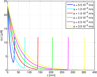
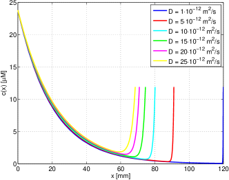
Figure 7: Concentration profiles in Case I.iv for varying $a$ and $D$, respectively.

Now we keep the ratio $c_{\mathrm{s}}/c_{\infty}=2$, i.e., $c_{\mathrm{s}}=2c_{\infty}=23.8\cdot 10^{-3}$ mol$/$m³ and vary the other steady-state parameters. This corresponds to Case I.iv in Theorem 4.1.

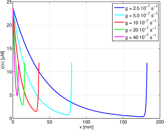
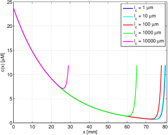
Figure 8: Concentration profiles in Case I.iv for varying $g$ and $l_{\mathrm{c}}$, respectively.

From Figure 7 we can conclude that the steady-state length $l_{\infty}$ increases with the active transport $a$ and both $l_{\infty}$ and the concentration profile $c(x)$ are sensitive to small variations in $a$. On the other hand, increasing the diffusion $D$ implies a decrease in $l_{\infty}$, but hardly changes $c(x)$, except near the growth cone. Decreasing $D$ means a substantial increase in $l_{\infty}$. Note that, according to Section 4.5, in the limit $D=0$ there exists generally no continuous steady-state solution. The physically relevant solution is given by (32), which is a decreasing function all the way to the steady-state length $l_{\infty}=184$ mm (for $c_{\mathrm{s}}/c_{\infty}=2$).

Given the nominal values of Table 1, Figure 8 shows that increasing the degradation rate $g$ implies a substantial decrease in $l_{\infty}$. However; the length $l_{\infty}$ is relatively insensitive to the size of the growth cone expressed by the parameter $l_{\mathrm{c}}$, unless this gets very big.

6 On the stability of the steady states

It is of interest to know whether a steady-state solution of a mathematical model is biologically and physically relevant, i.e., whether it can exist in reality. A steady-state solution of a model is stable if one uses a disturbance of the steady state as initial data and the dynamic solution converges back to the steady state. If the solution moves further away, the steady state is unstable.

Referring to the different cases of parameter values treated in the theorems of Section 4, we expect that when there exists a unique steady state, it is stable. However, in Case I.iii of Theorem 4.1, in which $f(z_{0})=0.06<c_{\mathrm{s}}/c_{\infty}<1$, there exist two steady states and the question is what happens for large times. Because of the presence of diffusion, which has a damping effect on any oscillation, it is reasonable to assume that the dynamic solution converges to a steady state as time increases.

Since it is difficult to make stability analyses mathematically, we make the investigations here numerically. McLean and Graham [12] make a spatial transformation so that the moving interval $(0,l(t))$ for the PDE is transformed to the fixed interval $(0,1)$. A numerical implementation for their problem is presented by Graham et al. [6]. The transformation means that the same number of spatial computational cells is used along the axon irrespective of its length. We will use the same spatial transformation:

$$y:=\frac{x}{l(t)},\qquad\frac{\partial{y}}{\partial{x}}=\frac{1}{l(t)},\qquad\frac{\partial{y}}{\partial{t}}=-\frac{xl^{\prime}(t)}{l(t)^{2}}=-\frac{yl^{\prime}(t)}{l(t)}.$$

With $\bar{c}(y,t):=c(yl(t),t)$, we get

$$\frac{\partial{c}}{\partial{t}}=\frac{\partial{\bar{c}}}{\partial{t}}-\frac{yl^{\prime}(t)}{l(t)}\frac{\partial{\bar{c}}}{\partial{y}},\qquad\frac{\partial{c}}{\partial{x}}=\frac{1}{l(t)}\frac{\partial{\bar{c}}}{\partial{y}},\qquad\frac{\partial^{2}c}{\partial x^{2}}=\frac{1}{l(t)^{2}}\frac{\partial^{2}\bar{c}}{\partial y^{2}}.$$

Then the dynamic model (14) is transformed to

$$\left\{\begin{aligned} &\frac{\partial{\bar{c}}}{\partial{t}}+\alpha(y,c_{\mathrm{c}},l)\frac{\partial{\bar{c}}}{\partial{y}}-\frac{D}{l^{2}}\frac{\partial^{2}\bar{c}}{\partial y^{2}}=-g\bar{c},&\quad&0<y<1,\ t>0,\\ &\begin{split}&\frac{\mathrm{d}{c_{\mathrm{c}}}}{\mathrm{d}{t}}=\frac{(a-gl_{\mathrm{c}})}{l_{\mathrm{c}}}c_{\mathrm{c}}-\frac{D}{l_{\mathrm{c}}l}\bar{c}_{y}^{-}\\ &\qquad-\frac{(r_{\mathrm{g}}c_{\mathrm{c}}+\tilde{r}_{\mathrm{g}}l_{\mathrm{c}})}{l_{\mathrm{c}}}(c_{\mathrm{c}}-c_{\infty}),\end{split}&&t>0,\\ &\frac{\mathrm{d}{l}}{\mathrm{d}{t}}=r_{\mathrm{g}}(c_{\mathrm{c}}-c_{\infty}),&&t>0,\\ &\bar{c}(0,t)=c_{\mathrm{s}}(t),&&t\geq 0,\\ &\bar{c}(1,t)=c_{\mathrm{c}}(t),&&t>0,\\ &\bar{c}(y,0)=c_{0}(yl_{0}),&&0\leq y\leq 1,\\ &c_{\mathrm{c}}(0)=c_{0}(l_{0}),&&\\ &l(0)=l_{0},&&\end{aligned}\right.$$ (34)

where

$$\alpha\big{(}y,c_{\mathrm{c}}(t),l(t)\big{)}:=\frac{a-yl^{\prime}(t)}{l(t)}=\frac{a-yr_{\mathrm{g}}\big{(}c_{\mathrm{c}}(t)-c_{\infty}\big{)}}{l(t)}.$$

We will find approximate solutions to the model (34) using the method of lines by performing a spatial discretization of the PDE. The $y$-interval $[0,1]$ is divided into $M$ subintervals all of the size $\Delta y:=1/M$. Set $y_{j}:=j\Delta y$ and let $\bar{C}_{j}\approx\bar{c}(y_{j},t)$ for $j=0,\ldots,M$, where $\bar{C}_{M}(t)=c_{\mathrm{c}}(t)$ by the continuity boundary condition. Spatial second-order difference approximations are used:

$$\frac{\partial{\bar{c}}}{\partial{y}}(y_{j},\cdot)\approx\frac{\bar{C}_{j+1}-\bar{C}_{j-1}}{2\Delta y},\quad\frac{\partial^{2}\bar{c}}{\partial y^{2}}(y_{j},\cdot)\approx\frac{\bar{C}_{j+1}-2\bar{C}_{j}+\bar{C}_{j-1}}{(\Delta y)^{2}}.$$

In the ODE for the cone concentration, we use the one-sided second order approximation

$$\bar{c}_{y}^{-}\approx\frac{\bar{C}_{M}-4\bar{C}_{M-1}+3\bar{C}_{M-2}}{2\Delta y}=\frac{c_{\mathrm{c}}-4\bar{C}_{M-1}+3\bar{C}_{M-2}}{2\Delta y}.$$

Denote the time step by $\Delta t$ and set $t^{n}:=n\Delta t$, $n=0,1,\ldots$. At time $t=t^{n}$, the concentration within the axon is approximated by the numerically computed values $\bar{C}_{j}^{n}\approx\bar{c}(y_{j},t^{n})$, $j=1,\ldots,M-1$. The approximate growth-cone concentration is denoted by $C_{\mathrm{c}}^{n}\approx\bar{c}_{\mathrm{c}}(t^{n})$, the axon length by $L^{n}\approx\bar{l}(t^{n})$. The explicit Euler method means that each time derivative is approximated by formulas like

$$\frac{\partial{\bar{c}}}{\partial{t}}(y_{j},t^{n})\approx\frac{\bar{C}_{j}^{n+1}-\bar{C}_{j}^{n}}{\Delta t}.$$

As initial values, we set

$$\bar{C}_{j}^{0}=c_{0}(y_{j}l_{0}),\quad j=1,\ldots,M,\quad C_{\mathrm{c}}^{0}=c_{0}(l_{0})\quad\text{and}\quad L^{0}=l_{0}.$$

Substituting the approximations of the derivatives into (34) we get an explicit time marching numerical method, i.e., only old values of the unknowns are used. For example, the update formulas for the concentration values along the axon are, for $j=1,\ldots,M-1$:

$$\begin{split}\bar{C}_{j}^{n+1}&=\bar{C}_{j}^{n}+\Delta t\left(-\alpha(y_{i},C_{\mathrm{c}}^{n},L^{n})\frac{\bar{C}^{n}_{j+1}-\bar{C}^{n}_{j-1}}{2\Delta y}\right.\\ &\qquad\qquad+\left.\frac{D}{(L^{n})^{2}}\frac{\bar{C}_{j+1}^{n}-2\bar{C}_{j}^{n}+\bar{C}_{j-1}^{n}}{(\Delta y)^{2}}-g\bar{C}_{j}^{n}\right)\end{split}$$

$$\begin{split}&=\left(1-\Delta t\left(\frac{2D}{(L^{n}\Delta y)^{2}}-g\right)\right)\bar{C}_{j}^{n}\\ &\qquad+\Delta t\left(-\frac{\alpha(y_{i},C_{\mathrm{c}}^{n},L^{n})}{2\Delta y}+\frac{D}{(L^{n}\Delta y)^{2}}\right)\bar{C}^{n}_{j+1}\\ &\qquad\qquad+\Delta t\left(\frac{\alpha(y_{i},C_{\mathrm{c}}^{n},L^{n})}{2\Delta y}+\frac{D}{(L^{n}\Delta y)^{2}}\right)\bar{C}^{n}_{j-1}.\end{split}$$ (35)

Given $\Delta y=1/M$, the time step $\Delta t$ has to be chosen sufficiently small to avoid instabilities in the updates (35) for the advection-diffusion PDE of (34). For example, with constant Dirichlet boundary conditions, there exists a standard so called CFL condition to ensure stability. The complication here is the coupling to the two ODEs via the boundary at $x=l(t)$. Therefore, we make some assumptions on the numerical updates. To be more precise, let $N$ be the number time steps, $T:=N\Delta t$ the total simulation time and set

$$c_{\mathrm{max}} :=\max\big{(}c_{\infty},\max\limits_{0\leq t\leq T}c_{\mathrm{s}}(t)\big{)}.$$

Assume that the numerical values satisfy

$$L^{n}\geq l_{\mathrm{min}}>0\quad\text{and}\quad 0\leq C_{\mathrm{c}}^{n}\leq c_{\mathrm{max}}\quad\text{for $n=0,1,\ldots,N$},$$ (36)

where $l_{\mathrm{min}}$ is a constant. The scheme (35) is monotone (or positive) if the coefficients for $\bar{C}^{n}_{j-1}$, $\bar{C}^{n}_{j}$ and $\bar{C}^{n}_{j+1}$ are non-negative. Then no unphysical numerical oscillations appear within the axon. The requirements on the discretization parameters are the cell Péclet condition for $\Delta y$ and a CFL condition for $\Delta t$:

$$\Delta y \leq\frac{2D}{(a+r_{\mathrm{g}}2c_{\mathrm{max}})l_{\mathrm{min}}},$$ (37)

$$\Delta t \leq\left(g+\frac{2D}{(l_{\mathrm{min}}\Delta y)^{2}}\right)^{-1}.$$ (38)

We first demonstrate Case I.iv of Theorem 4.1, which is the case when $c_{\mathrm{s}}/c_{\infty}>1$ and there exists a unique steady-state solution. To be able to compare with Figure 4, we choose the constant ratio $c_{\mathrm{s}}/c_{\infty}=2$ and the initial axon length $l(0)=2$ mm. With the spatial discretization $M=1/\Delta y=1000$, the stability criterion (37) is satisfied (with $l_{\mathrm{min}}=2$ mm) and the CFL condition (38) gives $\Delta t\leq 5.0$ s. The axon length as function of time is shown in Figure 9.

Figure 9: A dynamic simulation of the outgrowth of an axon when $c_{\mathrm{s}}/c_{\infty}=2$. According to the steady-state results in Section 4, the final length is $l_{\infty}=80.1$ mm and the final concentration distribution is the same as the theoretically obtained one in Figure 4.

In the following simulations, we have chosen $M=300$ and $\Delta t$ in accordance with (37)–(38). In the next two simulations, we choose $c_{\mathrm{s}}/c_{\infty}=0.1$, which corresponds to Case I.iii of Theorem 4.1 and means that there are two steady-state solutions; see the red and green dots in Figure 2 and the corresponding steady-state concentrations in Figure 3. The simulation shown in Figure 10 demonstrates simultaneously the instability of the steady state with the shorter length $l_{\infty}^{\mathrm{short}}=2.82$ mm and the stability of the longer one with $l_{\infty}^{\mathrm{long}}=17.3$ mm by starting very close to the smaller steady state: $l(0)=l_{\infty}^{\mathrm{short}}+1~{}\mu$m and with an initial profile $c(x,0)$ very close to $c_{1}(x)$ shown in Figure 3.

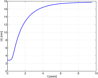
Figure 10: The case $c_{\mathrm{s}}/c_{\infty}=0.1$. Dynamic behaviour of an axon with initial length slightly larger than the steady-state value $l_{\infty}^{\mathrm{short}}=2.82$ mm. The initial data is almost in steady state, but since this is unstable, convergence to the other stable steady state occurs.

If the initial data is instead a small perturbation to the slightly shorter length $l(0)=l_{\infty}^{\mathrm{short}}-1~{}\mu$m, we get the simulation result in Figure 11.

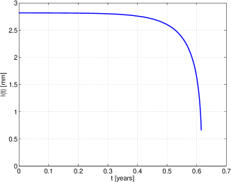
Figure 11: The case $c_{\mathrm{s}}/c_{\infty}=0.1$. The dynamic behaviour of an axon with initial length slightly smaller than the steady-state value $l_{\infty}^{\mathrm{short}}=2.82$ mm. The initial data is almost in steady state, but since this is unstable the axon shrinks.

Note that our model (14) is only valid for $l(t)>0$. In particular, zero length of an axon is not a steady state. This is in agreement with the simulation in Figure 11, in which $l^{\prime}(t)$ is far from zero as $l(t)\rightarrow 0$.

With the kept ratio $c_{\mathrm{s}}/c_{\infty}=0.1$, Figure 12 shows a simulation when the initial length is $l(0)=30$ mm, which is greater than the stable steady-state length $l_{\infty}^{\mathrm{long}}=17.3$ mm. There is a convergence back to the stable length 17.3 mm.

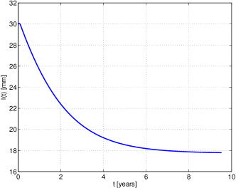
Figure 12: The case $c_{\mathrm{s}}/c_{\infty}=0.1$. Starting from the initial length of $l(0)=30$ mm there is a convergence to the steady-state length $l_{\infty}^{\mathrm{long}}=17.3$ mm.

Finally, we show a simulation when the initial length is $l(0)=30$ mm, but the ratio has been lowered to $c_{\mathrm{s}}/c_{\infty}=0.05$, which is below the threshold value $f(z_{0})=0.060$. According to Theorem 4.1 there exists no steady state, which is in accordance with the simulation in Figure 13, which shows how the axon shrinks.

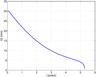
Figure 13: The case $c_{\mathrm{s}}/c_{\infty}=0.05$ when no steady state exists. Starting from the initial length of $l(0)=30$ mm the axons shrinks.

7 Discussion and conclusions

7.1 Mathematical modelling aspects

The dynamic model presented for axonal growth (14) can be seen as an extension and modification of a previously published model by McLean and Graham [12] (MG model). Both models use the linear PDE (5) for modelling the active and diffusive components of transport of tubulin along the axon and an ODE for the axonal elongation (12), namely that the length increase per time unit is equal to an affine relationship of the available concentration of free tubulin in the growth cone (or at the boundary $x=l(t)$).

The two new ingredients in our model is (1) an additional ODE for the concentration of free tubulin in the growth cone; and (2) a careful derivation of the flux of free tubulin into the growth — this flux includes the velocity of the moving boundary. We allow the growth cone to have a certain size, whereas it is zero in the MG model. When the size of the growth cone in our model tends to zero, the MG model is, however, not obtained. The reason lies in the ingredient (2). We explain this in detail below.

The MG model has an additional ODE for the production of tubulin in the soma. This means that the production rate and size of the soma must be known to drive the model. This is an interesting modelling aspect that we have purposely left out, since the boundary at $x=0$ is stationary and implies no special difficulty in the modelling. We have focused on the complexity of the moving boundary at $x=l(t)$ and have chosen the simpler assumption that the soma concentration is directly given as a function of time; $c_{\mathrm{s}}=c_{\mathrm{s}}(t)$.

In the modelling step, all the following phenomena or processes have been taken into account: active transport, diffusion, degradation along the axon and in the growth cone, assembly and disassembly of tubulin dimers in the growth cone and finally the movement of the growth cone, which is also the output of the model. The problematic fact is that all these effects are combined and influence each other, since they depend on the local concentration. With such many combined processes, it is impossible to tell beforehand (by physiological and biological experience) what a natural steady-state concentration distribution $c(x)$ along the axon is. It is then the strength of mathematical modelling comes in. Each phenomenon can be included individually, based on a restricted physiological or biological explanation possibly obtained from controlled experimental conditions; see Section 3 and all references therein. The outcome of the mathematical model is then the combination of all phenomena such that they obey the overall physical law of conservation of mass. A typical such example is the non-monotone concentration distribution of free tubulin $c(x)$ along the axon, which our model yields for nominal parameter values. Having a correct intuitive feeling for the final outcome would be equal to solving the differential equations by intuition. On the other hand, once we have the mathematical result (the non-monotone profile), one should try to give some intuitive explanations; see Section 7.2.

It is interesting to track down the exact details of the differences between the present model and the MG model. We use the same PDE (5) along the axon, which comes from the conservation of mass and the fact that the flux [mol/s] of tubulin at any fixed point on the $x$-axis is $ac^{-}-Dc_{x}^{-}$. We also use the same ODE for the axonal elongation (12). The second ODE in our model describes the accumulation of free tubulin in the growth cone and models thereby the dynamic variation of the cone concentration $c_{\mathrm{c}}(t)$. In this way, we get a natural connection between the transport processes along the axon and the growth cone concentration.

The MG model has a growth cone of size zero, which is a mathematical idealization that can be made. However, the main difference lies in the boundary condition at $x=l(t)$. We have carefully derived that the flux of tubulin over $x=l(t)$ (seen by an observer moving with the boundary) is given by the expression (7), i.e., the flux per area unit [mol/(m²s)] is $ac^{-}-Dc_{x}^{-}-l^{\prime}(t)c^{-}$. McLean and Graham [12] writes that this flux is $-c_{x}^{-}$. Hence, they assume that diffusion is the only effective flux (with $D=1$) and that $a=l^{\prime}(t)$. (The latter equality implies $l(t)=at+l_{0}$, which contradict the ODE for $l(t)$.) In any case, their final boundary condition [12, Equation (2.3)] for $x=l(t)$ is

$$c_{x}^{-}=-\epsilon_{l}c^{-}+\zeta_{l}.$$ (39)

This introduction of new parameters remove the above implicit assumption that $D=1$. However, (39) means that the moving boundary has not been taken into account. To compare with our model, Equation (39) can be seen as a simplification of our ODE for the growth cone concentration, which is either (8), (13) or the second equation of (14). Namely, setting the size parameter $l_{\mathrm{c}}$ of the growth cone to zero and using $c_{\mathrm{c}}=c^{-}$, (13) becomes

$$0=ac^{-}-Dc_{x}^{-}-r_{\mathrm{g}}(c^{-}-c_{\infty})c^{-}\quad\Longleftrightarrow\quad$$

$$c_{x}^{-}=-\frac{r_{\mathrm{g}}}{D}(c^{-})^{2}+\frac{a+r_{\mathrm{g}}c_{\infty}}{D}c^{-}.$$ (40)

An equivalent way of obtaining this equation is to simply use the conservation of mass over $x=l(t)$. Seen from an observer moving with the boundary (to the right along the $x$-axis), the influx on the left-hand side of $x=l(t)$ is $ac^{-}-Dc_{x}^{-}-l^{\prime}(t)c^{-}$, which is equal to the flux out on the right-hand side, which is zero. Substituting the ODE for $l^{\prime}(t)$ one arrives at (40).

The differences between the two models (when the growth cone has zero size) can now be seen in the differences between (39) and (40). Firstly, in (40) no new parameter has been introduced, in contrast to $\epsilon_{l}$ and $\zeta_{l}$ (39). Secondly, taking the moving boundary into account, one ends up in a nonlinear relation (40) between the concentration $c^{-}$ and its spatial derivative $c_{x}^{-}$. This difference explains why the MG model yields decreasing concentration profiles along the axon, whereas we get non-monotone ones.

Note that we get a non-monotone profile also in the case when $l_{\mathrm{c}}=0$; Theorem 4.1 still holds; see also Figure 8. Then there is no ODE for the growth cone, but instead the boundary condition (40) at $x=l(t)$ for the PDE. Hence, it is not the growth cone ODE that is responsible for the non-monotone steady-state profile, it is simply the outcome of the conservation law of mass.

7.2 Conclusions

One outcome of this work is the presented new dynamic model of tubulin-driven axonal growth (14). The input to the model is the tubulin concentration $c_{\mathrm{s}}(t)$, which we assume is given. Except for this function, the model has seven (constant) parameters, which are all biological or physiological parameters or combinations of such. Since we analyze steady-state solutions in this work, $c_{\mathrm{s}}$ has been constant in time. Depending on this value, and the values of five additional parameters ($a$, $D$, $g$, $l_{\mathrm{c}}$, $c_{\infty}$), all steady-state solutions have been classified. One conclusion is that the values of the rate constants $r_{\mathrm{g}}$ and $\tilde{r}_{\mathrm{g}}$ in the dynamic model have no influence on the steady states, hence only on the dynamic behaviour and convergence to steady state.

The biologically most interesting cases arise when all parameters take positive values and these cases are given in Theorem 4.1. With the nominal parameter values (Table 1), which we have extracted directly or indirectly from the biological literature, the following inequality is fulfilled:

$$gl_{\mathrm{c}}=2\cdot 10^{-12}\text{~{}m$/$s}~{}<1\cdot 10^{-8}\text{~{}m$/$s~{}}=a.$$

Then Case I of Theorem 4.1 states that, when a steady state exists, the concentration of tubulin along the axon $c(x)$ is given by the explicit formula (27), but the length $l_{\infty}$ has to be obtained numerically by solving the equation $f(z)=c_{\mathrm{s}}/c_{\infty}$ with $f(z)$ given by (24). A way of getting an overview of the possible values of $l_{\infty}$ is to plot the graph of the function (24), which has a minimum at $z_{0}=5.64$ mm; see Figure 2. The value on the ratio $c_{\mathrm{s}}/c_{\infty}$ gives directly whether zero, one or two steady states exist and the corresponding length(s) $l_{\infty}$ can be read off on the $z$-axis. If the ratio $c_{\mathrm{s}}/c_{\infty}<f(z_{0})=0.06$, then there exists no steady state, i.e. no outgrowth can occur. For higher values on $c_{\mathrm{s}}/c_{\infty}$, the steady-state concentration along the axon is given by the function (27). If $0.06<c_{\mathrm{s}}/c_{\infty}<1$, then there exists two steady-state solutions. One has a very short $l_{\infty}<z_{0}=5.64$ mm, which actually becomes smaller and smaller the closer the ratio $c_{\mathrm{s}}/c_{\infty}$ is to 1. Dynamic numerical simulations indicate that this is an unstable steady state and thus not possible biologically. The other steady state is stable, has a larger $l_{\infty}>z_{0}=5.64$ mm, and this value is larger the larger $c_{\mathrm{s}}/c_{\infty}$ is. When $c_{\mathrm{s}}/c_{\infty}\geq 1$, there exists a unique steady-state solution.

Numerical simulations of the dynamic behaviour in Section 6 indicate that every steady-state solution with $l_{\infty}>z_{0}=5.64$ mm is stable, whereas the shorter ones are unstable. An overall conclusions is thus that for the most interesting cases when $gl_{\mathrm{c}}<a$ and $c_{\mathrm{s}}/c_{\infty}>f(z_{0})$ hold, there exists a unique stable steady-state solution. For an axon of arbitrary length, if the soma concentration decreases to a constant value such that $c_{\mathrm{s}}/c_{\infty}<f(z_{0})$, then there exists no steady-state solution and dynamic numerical simulations show a shrinking axon.

One interesting outcome from the model is the form of the concentration distribution $c(x)$ along the axon for the stable steady states in Case I of Theorem 4.1. Starting from the soma at $x=0$, the concentration decreases and is in fact along a large portion of the axon lower than both $c_{\mathrm{s}}$ and the steady-state soma concentration $c_{\infty}$. The explanation for this form is hard to make intuitively, since it is a result of the combined effects of active transport, diffusion, degradation, (dis)assembly of tubulin and the velocity of the growth cone. The mathematical equations combine these phenomena and yield the very form of $c(x)$, which is given explicitly by the closed-form expression (27). This is a good example of the purpose and strength of mathematical modelling; it is impossible to reason biologically what the precise form of a steady-state solution should be.

An interesting biological conclusion, which is in agreement with experimental results, is that a relatively large active transport velocity $a$ means that the flux is sufficiently large to transport tubulin the long way out to the growth cone despite the relatively low concentration of tubulin in the axon. Along the axon, the two flux components, advective and diffusive, are precisely balanced by the degradation of tubulin. Note that the total flux (advective plus diffusive) is decreasing along the axon because of the degradation. The increasing concentration distribution near the growth cone implies that diffusion occurs in the direction to the soma but the active transport to the growth cone is so large that the net flux is precisely what is needed to balance the degradation of tubulin in the growth cone. Note also that we have assumed that the concentration of tubulin varies continuously due to the presence of diffusion.

If the active transport velocity $a$ is too low, namely less than $gl_{\mathrm{c}}$ (Case II of Theorem 4.1), then there still exists a unique solution; however, the concentration along the axon $c(x)$ is decreasing, which partly means that the diffusion flux is always directed towards to growth cone, and partly that this solution only exists if the soma concentration $c_{\mathrm{s}}>c_{\infty}$.

The model gives information also in the extreme cases when one or more parameters are zero. The biological interest in such cases is if the corresponding variable(s) are negligible. The mathematical advantage to set a very small variable to zero, is that in some cases one gets special solutions that can be written up explicitly which makes it easier to draw biological conclusions.

When advection is negligible ($a=0$), the flux of tubulin from the soma to the growth cone is only present in the form of diffusion. Since diffusive flux occurs from higher to lower concentrations, the only possible steady state has a decreasing concentration of tubulin from the soma to the growth cone, which is precisely what Theorem 4.2 states. This theorem also states that if the soma concentration is too small ($c_{\mathrm{s}}<c_{\infty}$), there exists no steady state with $l_{\infty}>0$.

Another extreme case is when the degradation of tubulin is negligible ($g=0$). Theorem 4.3 states that a steady state exists if and only if $c_{\mathrm{s}}<c_{\infty}$ holds. Then there is no net flux at any $x$ along the axon; i.e. the concentration $c(x)$ is increasing in such away that the advective flux towards the growth cone is equal to the diffusive flux back to the soma. If $c_{\mathrm{s}}\geq c_{\infty}$, then there exists no steady state and the the axon may grow indefinitely.

The case when diffusion is negligible ($D=0$) is a special case; however, not an unrealistic case, since $D$ is a relatively small number. Without diffusion, the solution of the PDE may in fact contain discontinuities. Hence, the continuity assumption we have made for the boundary conditions is not natural. From a mathematical point of view, one cannot beforehand ignore the possibility of a concentration discontinuity at $x=l(t)$. Theorem 4.4 gives explicit functions for both the decreasing concentration profile along the axon and the length of the axon in the unique steady state. Note that the decreasing concentration along the axon agrees with the general case except near the growth cone. We also note that the steady state exists if and only if $ac_{\mathrm{s}}>gl_{\mathrm{c}}c_{\infty}$, i.e., when the advective flux ($ac_{\mathrm{s}}$) from the soma is greater than the degradation of tubulin in the growth cone ($gl_{\mathrm{c}}c_{\infty}$). The difference between these two numbers is precisely the amount per time unit of transported tubulin along the axon that is degraded.

We have not found (in literature) any experimental indications against the non-monotone concentration distribution of tubulin along the axon which our model yields for the nominal parameter values. It is in agreement with the fact that the active transport is the most important ingredient for the outgrowth of long axons. The velocity $a$ of the active transport has been assumed to be constant. Experiments reported by Watson et al. [29] and Xu and Tung [30] show a decreasing velocity along fully grown axons; i.e. $a=a(x)$ is a decreasing function. Although such a dependence could be included in the model, it is not clear what causes this decrease and hence what function $a(x)$ to use.

More comprehensive future extensions of the model would be to include other substances than tubulin, for example, actin which is redistributed within the growth cone so that it can turn as a response to external stimuli.

References

- [1] M. Caplow and L. Fee. Dissociation of the tubulin dimer is extremely slow, thermodynamically very unfavorable, and reversible in the absence of an energy source. Mol. Biol. Cell, 13(6):2120–2131, 2002.
- [2] E. W. Dent and F. B. Gertler. Cytoskeletal dynamics and transport in growth cone motility and axon guidance. Neuron, 40(2):209–227, 2003.
- [3] J. A. Galbraith and P. E. Gallant. Axonal transport of tubulin and actin. J. Neurocytology, 29(11–12):889–911, 2000.
- [4] J. A. Galbraith, T. S. Reese, M. L. Schlief, and P. E. Gallant. Slow transport of unpolymerized tubulin and polymerized neurofilament in the squid giant axon. Proceedings of the National Academy of Sciences of the United States of America, 96(20):11589–11594, 1999.
- [5] J. A. García, J. M. Peña, S. McHugh, and A. Jérusalem. A model of the spatially dependent mechanical properties of the axon during its growth. CMES – Computer Modeling Eng. Sci., 87(5):411–432, 2012.
- [6] B. P. Graham, K. Lauchlan, and D. R. McLean. Dynamics of outgrowth in a continuum model of neurite elongation. J. Comput. Neuroscience, 20(1):43–60, 2006.
- [7] B. P. Graham and A. van Ooyen. Mathematical modelling and numerical simulation of the morphological development of neurons. BMC Neuroscience, 7(SUPPL. 1), 2006.
- [8] J. J. Johannes Hjorth, Jaap van Pelt, Huibert D. Mansvelder, and Arjen van Ooyen. Competitive dynamics during resource-driven neurite outgrowth. PLoS ONE, 9(2):e86741, 02 2014.
- [9] A. Janulevicius, J. van Pelt, and A. van Ooyen. Compartment volume influences microtubule dynamic instability: A model study. Biophys. J., 90(3):788–798, 2006.
- [10] C. H. Keith. Slow transport of tubulin in the neurites of differentiated PC12 cells. Science, 235(4786):337–339, 1987.
- [11] G. Kiddie, D. McLean, A. Van Ooyen, and B. Graham. Biologically plausible models of neurite outgrowth. In C. N. Levelt A. van Ooyen G. J. A. Ramakers J. van Pelt, M. Kamermans and P. R. Roelfsema, editors, Development, Dynamics and Pathiology of Neuronal Networks: from Molecules to Functional Circuits, volume 147 of Progress in Brain Research, pages 67–80. Elsevier, 2005.
- [12] D. R. McLean and B. P. Graham. Mathematical formulation and analysis of a continuum model for tubulin-driven neurite elongation. Proceedings Royal Society A: Mathematical, Physical and Engineering Sciences, 460(2048):2437–2456, 2004.
- [13] D. R. McLean and B. P. Graham. Stability in a mathematical model of neurite elongation. Math. Med. Biol., 23(2):101–117, 2006.
- [14] D. R. McLean, A. van Ooyen, and B. P. Graham. Continuum model for tubulin-driven neurite elongation. Neurocomputing, 58–60:511–516, 2004.
- [15] K. E. Miller and S. R. Heidemann. What is slow axonal transport? Exp. Cell Res., 314(10):1981–1990, 2008.
- [16] K. E. Miller and D. C. Samuels. The axon as a metabolic compartment: Protein degradation, transport, and maximum length of an axon. J. Theor. Biol., 186(3):373–379, 1997.
- [17] T. Mitchison and M. Kirschner. Dynamic instability of microtubule growth. Nature, 312(5991):237–242, 1984.
- [18] M. O’Toole and K. E. Miller. The role of stretching in slow axonal transport. Biophys. J., 100(2):351–360, 2011.
- [19] R. Pepperkok, M. H. Bre, J. Davoust, and T. E. Kreis. Microtubules are stabilized in confluent epithelial cells but not in fibroblasts. J. Cell Biol., 111(6 II):3003–3012, 1990.
- [20] K. Sadegh Zadeh and S. B. Shah. Mathematical modeling and parameter estimation of axonal cargo transport. J. Comp. Neurosci., 28(3):495–507, 2010.
- [21] E. D. Salmon, W. M. Saxton, R. J. Leslie, M. L. Karow, and J. R. McIntosh. Diffusion coefficient of fluorescein-labeled tubulin in the cytoplasm of embryonic cells of a sea urchin: Video image analysis of fluorescence redistribution after photobleaching. J. Cell Biol., 99(6):2157–2164, 1984.
- [22] D. A. Smith and R. M. Simmons. Models of motor-assisted transport of intracellular particles. Biophys. J., 80(1):45–68, 2001.
- [23] D. M. Suter and K. E. Miller. The emerging role of forces in axonal elongation. Progress Neurobiol., 94(2):91–101, 2011.
- [24] E. Tanaka and J. Sabry. Making the connection: Cytoskeletal rearrangements during growth cone guidance. Cell, 83(2):171–176, 1995.
- [25] A. van Ooyen. Using theoretical models to analyse neural development. Nature Reviews Neuroscience, 12(6):311–326, 2011.
- [26] A. van Ooyen, B. P. Graham, and G. J. A. Ramakers. Competition for tubulin between growing neurites during development. Neurocomputing, 38–40(0):73–78, 2001.
- [27] M. P. Van Veen and J. Van Pelt. Neuritic growth rate described by modeling microtubule dynamics. Bull. Math. Biology, 56(2):249–273, 1994.
- [28] R. A. Walker, E. T. O’Brien, N. K. Pryer, M. F. Soboeiro, W. A. Voter, H. P. Erickson, and E. D. Salmon. Dynamic instability of individual microtubules analyzed by video light microscopy: rate constants and transition frequencies. J. Cell Biol., 107(4):1437–1448, 1988.
- [29] D. F. Watson, P. N. Hoffman, K. P. Fittro, and J. W. Griffin. Neurofilament and tubulin transport slows along the course of mature motor axons. Brain Res., 477(1–2):225–232, 1989.
- [30] Z. Xu and V. W.-Y Tung. Temporal and spatial variations in slow axonal transport velocity along peripheral motoneuron axons. Neuroscience, 102(1):193–200, 2001.