Generation of cubic graphs and snarks with large girth

Abstract

We describe two new algorithms for the generation of all non-isomorphic cubic graphs with girth at least $k\geq 5$ which are very efficient for $5\leq k\leq 7$ and show how these algorithms can be efficiently restricted to generate snarks with girth at least $k$.

Our implementation of these algorithms is more than $30$, respectively $40$ times faster than the previously fastest generator for cubic graphs with girth at least $6$ and $7$, respectively.

Using these generators we have also generated all non-isomorphic snarks with girth at least $6$ up to $38$ vertices and show that there are no snarks with girth at least $7$ up to $42$ vertices. We present and analyse the new list of snarks with girth 6.

1 Introduction

A cubic (or $3$-regular) graph is a graph where every vertex has degree 3. Cubic graphs have interesting applications in chemistry as they can be used to represent molecules (where the vertices are e.g. carbon atoms such as in fullerenes [20]). Cubic graphs are also especially interesting in mathematics since for many open problems in graph theory it has been proven that cubic graphs are the smallest possible potential counterexamples, i.e. that if the conjecture is false, the smallest counterexample must be a cubic graph. For examples, see [5].

For most problems the possible counterexamples can be further restricted to the subclass of cubic graphs which are not $3$-edge-colourable. Note that by Vizing’s classical theorem the chromatic index (i.e. the minimum number of colours required for a proper edge-colouring of a given graph) of a cubic graph must be 3 or 4. Therefore cubic graphs with chromatic index 3 are often called colourable and those with chromatic index 4 uncolourable. For most conjectures uncolourable cubic graphs with low connectivity or girth (i.e. the length of the shortest cycle of the graph) which are counterexamples can be reduced to smaller counterexamples by certain standard operations. So in order to avoid these trivial cases, the class of potential minimal counterexamples is usually further restricted to the class of snarks: cyclically 4-edge-connected uncolourable cubic graphs with girth at least 5. (Recall that a graph is called cyclically $k$-edge-connected if the deletion of fewer than $k$ edges does not disconnect the graph into components which each contain at least one cycle).

Several algorithms have already been developed for the generation of complete lists of cubic graphs and it can be considered as a benchmark problem in structure enumeration. The first complete lists of cubic graphs were already determined at the end of the 19th century by de Vries who determined all cubic graphs up to 10 vertices [11, 12].

The first computer approach dates from 1966 and was done by Ballaban who generated all cubic graphs up to 12 vertices [1]. In the following decades several other algorithms for generating all cubic graphs have been proposed, each of them faster than the previous algorithm. For a more detailed overview of the history of the generation of cubic graphs, we refer to [7].

The fastest algorithm up until recently was developed by the first author in 1992 [2] and it has been implemented in a program called minibaum. At that time it could be used to generate all (connected) cubic graphs up to 24 vertices and in the meantime (when faster computers became available) it has already been used to generate all cubic graphs up to 30 vertices.

In 1999 Meringer [26] published an efficient algorithm for the generation of general regular graphs (so not just $3$-regular graphs). This generator has been implemented in a program called genreg, but it is slower than minibaum for generating $3$-regular graphs.

Together with McKay [6] we presented a new construction algorithm for cubic graphs in 2011. This algorithm has been implemented in a program called snarkhunter and is significantly faster than minibaum.

The generation algorithm of snarkhunter was also adapted to efficiently restrict the generation to cubic graphs with girth at least 4 or 5. Also in these cases snarkhunter was faster than minibaum. The bounding criteria incorporated in snarkhunter can in principle also be applied to generate cubic graphs with larger lower bounds on the girth, but this pruning technique is likely to become much less efficient for larger girth.

Before [5], the only way to generate complete lists of snarks was to use a generator for all cubic graphs with girth at least $5$ and apply a filter for colourability and cyclic edge-connectivity. However as only a tiny fraction of the cubic graphs is uncolourable (e.g. only 0.00008% of the cubic graphs with girth at least $5$ and $32$ vertices are snarks), this is certainly not an efficient approach.

The generation algorithm of snarkhunter allowed a look-ahead which in many cases avoids the generation of cubic graphs which are $3$-edge-colourable. By using this specialised generation algorithm for snarks, together with Hägglund and Markström [5] we were able to generate all snarks up to $36$ vertices. Using these new lists of snarks, we tested several open conjectures and were able to refute 8 of them. So this shows that snarks are not only theoretically a good source for counterexamples to conjectures, but also in practice.

For several conjectures the girth condition for possible minimal counterexamples has been strengthened (e.g. for the cycle double cover conjecture Huck [14] has even proven that a smallest possible counterexample must be a snark with girth at least $12$). Furthermore even though only a tiny fraction of the cubic graphs are snarks, there are already $60~{}167~{}732$ snarks with $36$ vertices and testing conjectures on all of these snarks can be computationally very expensive or even infeasible. So it would be interesting to consider more restricted subclasses of snarks that still have the property that smallest possible counterexamples for a lot of conjectures are contained in it. Therefore the main focus of this paper is the generation of cubic graphs and snarks with girth at least $6$ or $7$.

In Section 2 we describe two new algorithms for the generation of all non-isomorphic (connected) cubic graphs with girth at least $k\geq 5$ which are very efficient for $5\leq k\leq 7$. In the same section we also show how both algorithms can be extended with look-aheads which often allow to avoid the generation of $3$-edge-colourable graphs such that snarks with girth at least $k$ can be generated more efficiently.

In Section 3.1 we report the results and running times of our implementation of these algorithms for $5\leq k\leq 7$. Our implementation is more than $30$, respectively $40$ times faster than the previously fastest generator for cubic graphs with girth at least $6$ and $7$, respectively. For $k=5$ the algorithm which we developed earlier jointly with McKay in [6] was already very efficient, so in this case the speedup of the new algorithm is smaller (about $40$%).

The generation algorithms can also be applied for $k>7$, but are less efficient for these cases. Therefore we only implemented these algorithms for $k\leq 7$. For the generation of cubic graphs with girth $k\geq 9$ the fastest method is that of McKay, Myrvold and Nadon [24].

In [5] it was already determined that there are only 3 snarks with girth at least $6$ up to $36$ vertices. The new generator enabled us to generate all non-isomorphic snarks with girth at least $6$ and $38$ vertices. There are exactly 39 such snarks and in Section 3.2 we present and analyse these snarks.

We also generated a sample of snarks (i.e. girth at least $5$) with $38$ vertices and a sample of snarks with girth at least $6$ and $40$ vertices. In these cases it was computationally infeasible to generate the complete sets. In Section 3.2 we also describe which conjectures we tested on these new lists of snarks.

Jaeger and Swart conjectured that all snarks have girth at most 6 [18]. Kochol disproved this conjecture by giving a method for constructing snarks with arbitrarily large girth [19]. However the smallest snark with girth $7$ is currently still unknown. The smallest snark with girth $7$ obtained by Kochol’s method has 298 vertices, but there is no reason to assume that this is the smallest snark with girth $7$.

Using the new generators, we show that there are no snarks with girth at least $7$ up to $42$ vertices.

2 Generation algorithms

2.1 Introduction

An insertion operation or expansion is an operation which constructs a larger graph from a given graph. We call the inverse operation a reduction.

Figure 1 shows the main construction operation used in [6]. Note that this operation adds 2 new vertices. As already mentioned in [6], this algorithm can easily be equipped with look-aheads to generate graphs with a given lower bound $k$ on the girth efficiently. This was implemented in the program snarkhunter [4] for $k=4$ and $5$. For $k>5$ this method would not be efficient.

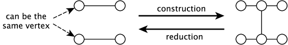
Figure 1: The basic edge insertion operation for cubic graphs used in [6].

As the number of cubic graphs grows very fast (see e.g. [27]), in algorithms which recursively construct cubic graphs from smaller cubic graphs, the most time consuming step is nearly always the last step.

Therefore in this paper we present two new algorithms which apply a special operation in the last step. The first algorithm which is described in Section 2.2 uses an operation that adds $4$ new vertices. We call it the tripod operation. The second algorithm which is described in Section 2.3 uses an operation that adds $6$ new vertices and we call it the $\mathcal{H}$ operation.

In both the tripod and $\mathcal{H}$ algorithm we use the canonical construction path method [23] to make sure that only pairwise non-isomorphic cubic graphs are generated. In order to use this method we have to define a canonical reduction which is unique up to isomorphism for every graph we want to generate. We call the expansion that is the inverse of a canonical reduction a canonical expansion. The two rules of the canonical construction path method are:

1. Only accept a graph if it was constructed by a canonical expansion.

2. For every graph $G$ to which construction operations are applied, only perform one expansion from each equivalence class of expansions of $G$.

The pseudocode for a general generation algorithm which uses the canonical construction path method is shown in Algorithm 1.

Algorithm 1 Construct(graph $G$)

  if $G$ has the desired number of vertices then

     output $G$

  else

     find expansions

     compute equivalence classes of expansions

     for each equivalence class do

        choose one expansion $X$

        perform expansion $X$

        if expansion $X$ was canonical then

           Construct(expanded graph)

        end if

        perform reduction $X^{-1}$

     end for

  end if

In Section 2.2 and 2.3 we will describe how we apply the canonical construction path method for the tripod and $\mathcal{H}$ algorithm, respectively and prove that exactly one representative of every isomorphism class of connected cubic graphs with girth at least $k$ is generated.

In those sections we will also show how both algorithms can be extended to generate snarks with girth at least $k$ significantly more efficiently than just filtering.

2.2 Tripod operation

2.2.1 Tripod operation for generating cubic graphs

Figure 2 shows the tripod operation. This operation subdivides the edges of a set of $3$ different edges (which we call an edge-triple) and inserts a $K_{1,3}$ between them. The edges of the edge-triple must be distinct, but they can have common vertices. This construction operation yields a cubic graph with $n+4$ vertices when applied to an edge-triple of a cubic graph with $n$ vertices.

We call the $K_{1,3}$ inserted by the tripod insertion operation a tripod and we call the vertex of degree 3 in the $K_{1,3}$ the central vertex of the tripod. The central vertex is labelled $c$ in Figure 2. Note that the central vertex of a tripod uniquely identifies the tripod.

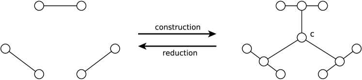
Figure 2: The tripod construction and reduction operation.

We call a tripod reducible if the central vertex of the tripod is not a cut vertex and each cycle with $i$ endvertices of the tripod has length at least $3+i$.

We define the edge-distance $d_{e}(e_{1},e_{2})$ between $2$ edges as the number of edges in a shortest path containing $e_{1}$ and $e_{2}$. The minimum edge-triple distance $d_{t}(e_{1},e_{2},e_{3})$ of an edge-triple $\{e_{1},e_{2},e_{3}\}$ is defined as $\min\{d_{e}(e_{1},e_{2}),d_{e}(e_{1},e_{3}),d_{e}(e_{2},e_{3})\}$. When applying a tripod operation to an edge-triple $\{e_{1},e_{2},e_{3}\}$ that inserts a new vertex $v$, $d_{e}(e_{i},e_{j})$ is equal to the usual distance $d(v_{i},v_{j})$ (that is: the number of edges in a shortest path from $v_{i}$ to $v_{j}$) in $G-v$ if $v_{i}$, respectively $v_{j}$ denote the vertices subdividing $e_{i}$ and $e_{j}$, respectively.

We say that two subgraphs of a graph are disjoint if they have no common vertices.

Theorem 1.

Every connected cubic graph $G$ with girth $k\geq 5$ has a reducible tripod.

The graph obtained by reducing a tripod has girth at least $k-1$ and at most $3$ disjoint cycles of length $k-1$.

Proof.

Every connected graph has a spanning tree and every tree with more than one vertex has at least two leaves. So every connected graph with at least $2$ vertices has at least $2$ vertices which are no cut vertices.

Choose an arbitrary vertex $v$ that is not a cut vertex as the central vertex of a tripod. Since $G$ has girth $k\geq 5$, each cycle with $i$ endvertices of the tripod has length at least $3+i$. As $G$ has girth $k$, any two neighbours of $v$ have distance at least $k-2$ in $G-v$, so any cycle in $G-v$ containing $m$ neighbours has length at least $\max\{k,(k-2)m\}$ leading to a cycle of length at least $\max\{k-m,(k-3)m\}\geq k-1$ in the reduced graph.

The last point follows immediately as in each cycle of length $k-1$ an edge must have been subdivided by a neighbour of $v$.

∎

So all connected cubic graphs with girth at least $k$ (for $k\geq 5$) with $n$ vertices can be obtained by applying the tripod operation to all possible edge-triples of connected cubic graphs with $n-4$ vertices in such a way that the tripod operation destroys all cycles of size smaller than $k$ without creating any new cycles of size smaller than $k$.

The following lemma follows directly from the definition of the tripod operation.

Lemma 2.

When applying the tripod expansion operation to the edge-triple $\{e_{1},e_{2},e_{3}\}$ of a graph $G$, the smallest cycle containing the central vertex of the tripod in the expanded graph has size $d_{t}(e_{1},e_{2},e_{3})+2$.

So more specifically, all cubic graphs with girth at least $k$ (for $k\geq 5)$ can be obtained by applying the tripod expansion operation to all possible edge-triples $\{e_{1},e_{2},e_{3}\}$ of cubic graphs with girth at least $k-1$ with at most 3 disjoint cycles of size $k-1$ for which $d_{t}(e_{1},e_{2},e_{3})\geq k-2$ and which destroy all cycles of size $k-1$. We call such edge-triples eligible edge-triples.

Now we still have to make sure that our algorithm does not output any isomorphic copies. We apply the canonical construction path method [23] to do this. We will now define what a canonical tripod expansion is and when expansions are considered equivalent. Then the two rules of the canonical construction path method applied to the tripod operation algorithm are as follows.

1. Only accept a cubic graph with girth at least $k$ if it was constructed by a canonical tripod expansion.

2. For every graph $G$ to which construction operations are applied, only perform one tripod expansion from each equivalence class of expansions of $G$.

Two edge-triples $\{e_{1},e_{2},e_{3}\}$ and $\{e_{1}^{\prime},e_{2}^{\prime},e_{3}^{\prime}\}$ of $G$ are called equivalent if there is an automorphism of $G$ mapping $\{e_{1},e_{2},e_{3}\}$ to $\{e_{1}^{\prime},e_{2}^{\prime},e_{3}^{\prime}\}$, i.e. if they are in the same orbit of edge-triples under the action of the automorphism group of $G$. We also denote the automorphism group of $G$ as $\operatorname{Aut}(G)$.

Recall from Section 2.1 that a canonical expansion is the inverse of a canonical reduction and that we have to define a canonical reduction which is unique up to isomorphism.

To define an efficient criterion for a tripod reduction of a graph $G$ to be canonical, we assign a 5-tuple $(x_{0},\dots,x_{4})$ to the central vertex $c$ of every reducible tripod and define an operation reducing the tripod with the smallest 5-tuple as the canonical reduction. The values of $x_{0},\ldots,x_{3}$ are combinatorial invariants of increasing discriminating power and cost and are defined as follows:

1. $x_{0}$ is the number of neighbours of $c$ which are part of a pentagon which does not contain $c$.

2. $x_{1}$ is the number of neighbours of $c$ which are part of a hexagon which does not contain $c$.

3. $x_{2}$ is the number of vertices at distance at most $3$ from $c$.

4. $x_{3}$ is the number of vertices at distance at most $4$ from $c$.

We chose these values of $x_{i}$ based on several performance tests comparing different choices for $x_{i}$.

Clearly, $x_{0}=0$ for all reducible tripods when generating graphs with girth at least $6$, so it does not discriminate between tripods and does not have to be computed. Analogously, $x_{0},x_{1}$ and $x_{2}$ do not have to be computed when generating graphs with girth at least $7$.

We call the tripod which was inserted by the last tripod insertion operation the inserted tripod. The value of $x_{i}$ only has to be computed for the reducible tripods which have the smallest value of $(x_{0},...,x_{i-1})$. Since we only need to know if the inserted tripod is canonical, we can stop as soon as we have found a reducible tripod with a smaller tuple $(x_{0},...,x_{i-1})$ (which implies that the inserted tripod is not canonical). We can also stop in case the inserted tripod is the only reducible tripod with the smallest value of $(x_{0},...,x_{i-1})$ (which implies that the inserted tripod is canonical).

Only in case there are multiple reducible tripods with the smallest value of $(x_{0},...,x_{3})$ (and the inserted tripod is one of them), we use the program nauty [22, 25] to compute a canonical labelling of the graph and define $x_{4}$ to be the smallest label in the canonical labelling of $G$ of a vertex which is in the same orbit of $\operatorname{Aut}(G)$ as $c$.

The discriminating power of $(x_{0},...,x_{3})$ is usually enough to decide whether or not the reduction is canonical, so the more expensive computation of $x_{4}$ can often be avoided. For example for generating connected cubic graphs with girth at least $6$ and $34$ vertices, the computation of $x_{4}$ is only required in about $4$% of the cases.

The definitions of $x_{0}$ and $x_{1}$ also allow look-aheads on level $n-4$ for deciding whether or not an expansion can be canonical before actually performing the tripod expansion operation. This allows to avoid the construction of a lot of graphs that would not be canonical. For example for generating connected cubic graphs with girth at least $6$ and $n$ vertices, these look-aheads allow to avoid the construction of about $89$% of the graphs for $n=34$. This percentage seems to be increasing for larger $n$.

Note that two vertices $v_{1},v_{2}$ have the same value for $(x_{0},...,x_{4})$ if and only if they are in the same orbit of the automorphism group of the graph.

Now we can prove the following theorem.

Theorem 3.

Assume that exactly one representative of each isomorphism class of connected cubic graphs with $n-4$ vertices with girth at least $k-1$ and at most 3 disjoint cycles of size $k-1$ is given. If we apply the following steps:

1. Apply the tripod insertion operation to one edge-triple in each orbit of eligible edge-triples.

2. Accept each graph with $n$ vertices if and only if the inserted tripod has minimal value of $(x_{0},\dots,x_{4})$ among all possible tripod reductions of the graph.

Then exactly one representative of each isomorphism class of connected cubic graphs with $n$ vertices and girth at least $k$ is accepted.

Proof.

First we will show that at least one representative of each isomorphism class of connected cubic graphs with $n$ vertices and girth at least $k$ is accepted.

Let $G$ be a connected cubic graph with $n$ vertices and girth at least $k$. It follows from Theorem 1 that $G$ has a reducible tripod, so also a canonical tripod reduction. Let $c$ be the central vertex of a canonical tripod of $G$ and we call the graph obtained by applying the tripod reduction to $c$ $p(G)$. The tripod of $G$ which was reduced corresponds to an edge-triple $\{e_{1},e_{2},e_{3}\}$ in $p(G)$.

By Theorem 1 $p(G)$ has girth at least $k-1$ and contains at most $3$ disjoint cyles of size $k-1$, so $p(G)$ is isomorphic to one of the input graphs $H$ to which the algorithm was applied. Let $\gamma$ be an isomorphism from $p(G)$ to $H$. The graph $H$ has an eligible edge-triple which is in the same orbit of edge-triples as $\gamma(\{e_{1},e_{2},e_{3}\})$ and the algorithm applies the tripod insertion operation to such an edge-triple. Let $c^{\prime}$ be the central vertex of the tripod obtained by applying the tripod expansion operation to this edge-triple in $H$. This produces a graph $G^{\prime}$ which is isomorphic to $G$, with an isomorphism $\gamma^{*}$ from $G$ to $G^{\prime}$ mapping $c$ to $c^{\prime}$. This implies that $c^{\prime}$ has a minimal value of $(x_{0},...,x_{4})$ and thus $G^{\prime}$ is accepted by the algorithm.

Now we will show that at most one representative of each isomorphism class of connected cubic graphs with $n$ vertices and girth at least $k$ is accepted.

Suppose the algorithm accepts two isomorphic graphs $G$ and $G^{\prime}$. Call the graphs obtained by applying a canonical tripod reduction to $G$ and $G^{\prime}$ $p(G)$ and $p(G^{\prime})$, respectively. Let $t$ be the canonical tripod which was reduced in $G$ and $t^{\prime}$ be the canonical tripod which was reduced in $G^{\prime}$ and let $\gamma$ be an isomorphism from $G$ to $G^{\prime}$. Since $t$ and $t^{\prime}$ are both canonical tripods, $\gamma(t)$ is in the same orbit as $t^{\prime}$ under the action of $\operatorname{Aut}(G^{\prime})$, so we can assume that $\gamma$ maps $t$ onto $t^{\prime}$. But this automorphism induces an isomorphism $\gamma_{p}$ from $p(G)$ to $p(G^{\prime})$. So by our assumption this means that $p(G)$ and $p(G^{\prime})$ are identical and that $\gamma_{p}$ is an automorphism mapping the edge-triple that was extended to form $G$ to the edge-triple that was extended to form $G^{\prime}$. This implies that equivalent edge-triples were extended – contradicting our assumption.

∎

To generate the connected cubic graphs with $n-4$ vertices with girth at least $k-1$, we used the efficient generator for cubic graphs described in [6] in case $k\leq 5$ or recursively apply the algorithm from Theorem 3 in case $k>5$.

It is also possible to incorporate look-aheads to avoid the generation of connected cubic graphs with $n-4$ vertices with girth at least $k-1$ with more than 3 disjoint cycles of size $k-1$. But in practice, this is not very helpful as the generation of cubic graphs with $n-4$ vertices and girth at least $k-1$ is usually not a bottleneck.

2.2.2 Tripod operation for generating snarks

In this section we describe how a look-ahead for the tripod operation can be used which often allows to avoid the generation of $3$-edge-colourable graphs.

Note that the application of the edge tripod insertion operation to an edge-triple can also be seen as first applying the edge insertion operation from Figure 1 to two of these edges and then applying the edge insertion operation to the new edge and the third edge.

Given a cubic graph $G$ and let $c:E(G)\to\{1,2,3\}$ be a proper $3$-edge-colouring of $G$. We call a cycle of $G$ where all edges have one of two colours $c_{1},c_{2}$ in the $3$-edge-colouring $c$ of $G$ a colour cycle or more specifically a $(c_{1},c_{2})$-cycle.

In [5], jointly with Hägglund and Markström we used the following well-known fact to avoid the generation of a lot of $3$-edge-colourable graphs using the edge insertion operation:

Theorem 4.

Given a cubic graph $G$ and a $3$-edge-colouring of $G$. If two edges $e,e^{\prime}$ belong to the same colour cycle (or equivalently: there is a path containing $e,e^{\prime}$ using only edges of two different colours), the graph $G^{\prime}$ obtained by applying the edge insertion operation from Figure 1 to $e,e^{\prime}$ will be $3$-edge-colourable.

Definition 5.

Let $\{e_{1},e_{2},e_{3}\}$ be an edge-triple in a $3$-edge-coloured cubic graph and $\{c_{1},c_{2},c_{3}\}=\{1,2,3\}$.

A $(c_{1},c_{2})$-path from an edge $e_{1}$ coloured with $c_{1}$ to an edge $e_{2}$ is a path starting with $e_{1}$ and ending with $e_{2}$, that contains only edges with colours $c_{1}$ and $c_{2}$. Note that the colour of $e_{2}$ can be both $c_{1}$ and $c_{2}$.

• A prune-path for $\{e_{1},e_{2},e_{3}\}$ is a path from $e_{1}$ to $e_{3}$ containing $e_{2}$, so that the path contains a $(c_{2},c_{1})$-path from $e_{2}$ to $e_{1}$ and a $(c_{2},c_{3})$-path from $e_{2}$ to $e_{3}$.

• Let $T$ be a tree with $3$ leaves contained in the edges $\{e_{1},e_{2},e_{3}\}$ so that $e_{1}$ also contains the (unique) vertex $v$ of degree $3$ and is coloured with $c_{1}$. If the path starting in the vertex $v$ and ending with $e_{2}$ is a $(c_{2},c_{1})$-path and the path starting in the vertex $v$ and ending with $e_{3}$ is a $(c_{3},c_{2})$-path, the tree $T$ is called a prune-tree for $\{e_{1},e_{2},e_{3}\}$.

In the following theorem we present a look-ahead for $3$-edge-colourability for the tripod insertion operation.

Theorem 6.

Given a cubic graph $G$, a $3$-edge-colouring $c$ of $G$ and edges $\{e_{1},e_{2},e_{3}\}$ in $G$.

If there is a prune-path or a prune-tree for $\{e_{1},e_{2},e_{3}\}$, then the graph obtained by applying a tripod operation to $\{e_{1},e_{2},e_{3}\}$ is $3$-edge-colourable.

Proof.

Applying the tripod operation to $\{e_{1},e_{2},e_{3}\}$ is equivalent to first applying the edge insertion operation from Figure 1 to $e_{1},e_{2}$ and then to the new edge and $e_{3}$.

If there is a prune-path for $\{e_{1},e_{2},e_{3}\}$ with a $(c_{2},c_{1})$-path from $e_{2}$ to $e_{1}$, then in the graph obtained by applying the edge insertion operation to $e_{1},e_{2}$, there is a $(c_{3},c_{2})$-path from the new edge to $e_{3}$ for the colouring shown in Figure 3.

If there is a prune-tree for $\{e_{1},e_{2},e_{3}\}$ with $e_{1}$ adjacent to the vertex of degree $3$ and a $(c_{1},c_{2})$-path from $e_{1}$ to $e_{2}$, then there is a $(c_{3},c_{2})$-path from the new edge to $e_{3}$ in the graph obtained by applying the edge insertion operation to $e_{1},e_{2}$ for the colouring shown in Figure 4.

In each case the graph after applying both edge insertion operations is $3$-edge-colourable by Theorem 4.

∎

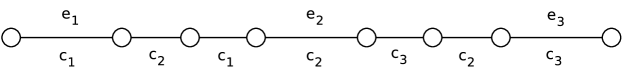
(a)

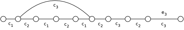
(b)

Figure 3: Procedure to recolour a prune-path when applying the tripod insertion operation to an edge-triple $\{e_{1},e_{2},e_{3}\}$ used in the proof of Theorem 6.

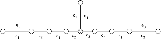
(a)

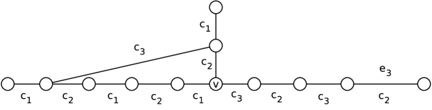
(b)

Figure 4: Procedure to recolour a prune-tree when applying the tripod insertion operation to an edge-triple $\{e_{1},e_{2},e_{3}\}$ used in the proof of Theorem 6.

We apply this look-ahead as follows for generating snarks with $n$ vertices and girth at least $k$. When a cubic graph $G$ with $n-4$ vertices and girth at least $k-1$ with at most $3$ disjoint cycles of size $k-1$ is generated, we compute three different $3$-edge-colourings of $G$. The look-ahead is only applicable if $G$ is $3$-edge-colourable, but this is not an issue as nearly all cubic graphs are $3$-edge-colourable [28]. We then mark all edge-triples which fulfil the conditions of Theorem 4 for one of the colourings. This allows to discard about $94$% of the edge-triples which would otherwise be expanded for $k=6$ and $n=36$.

The cost for computing a fourth colouring turned out to be higher than the gain achieved by the additionally discarded edge-triples. Actually after each colouring we first discard edge-triples and only compute the next colouring if there are sufficiently many eligible edge-triples left.

Theorem 6 is only applicable for the last step (i.e. the tripod operation), but as the number of graphs grows very fast, this already gives a considerable speedup as will be seen in Section 3.

2.3 $\mathcal{H}$ operation

2.3.1 $\mathcal{H}$ operation for generating cubic graphs

Figure 5 shows the $\mathcal{H}$ operation. We call a set $\{\{e_{1},e_{2}\},\{e_{3},e_{4}\}\}$ of two sets, each containing two edges and with all four edges pairwise different an edge-quadruple. This operation subdivides the edges of an edge-quadruple $\{\{e_{1},e_{2}\},\{e_{3},e_{4}\}\}$ and inserts an $\mathcal{H}$ graph between them. An $\mathcal{H}$ graph is a tree of 6 vertices with 2 adjacent vertices of degree 3. This construction operation yields a cubic graph with $n+6$ vertices when it is applied to an edge-quadruple of a cubic graph with $n$ vertices.

We call the edge where both vertices have degree 3 in the $\mathcal{H}$ graph the central edge of the $\mathcal{H}$. The central edge is labelled $e_{c}$ in Figure 5. Note that the central edge of an $\mathcal{H}$ uniquely identifies the $\mathcal{H}$.

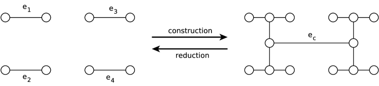
Figure 5: The $\mathcal{H}$ construction and reduction operation.

Let $G[S]$ denote the subgraph of a graph $G$ induced by the set of vertices $S\subseteq V(G)$. Given a connected graph $G$. We call an edge $e=\{x,y\}$ good if $G[V(G)-\{x,y\}]$ is connected. We call an $\mathcal{H}$ reducible if the central edge of the $\mathcal{H}$ is good and each cycle with $i$ endvertices of $\mathcal{H}$ has length at least $3+i$.

The following definitions and lemmas are needed for the proof that every connected cubic graph with girth at least $5$ has a reducible $\mathcal{H}$.

Lemma 7.

Every connected cubic graph has a good edge.

Proof.

De Vries [11, 12] has shown that every connected cubic graph can be obtained by recursively applying the construction operations from Figure 6 to a $K_{4}$.

$K_{4}$ has $6$ good edges, so it is sufficient to show that when applying the operations to a graph with good edges, the result has good edges too. Operation (a) adds a subgraph that contains $5$ good edges, so the result of applying this operation always has good edges. When operation (b) or (c) are applied, good edges not involved in the operation stay good, so assume that a good edge is involved in the operation.

For (b) it is easy to see that in this case all newly inserted edges are good, while for (a) both parts of the good edge that was subdivided are new good edges.

∎

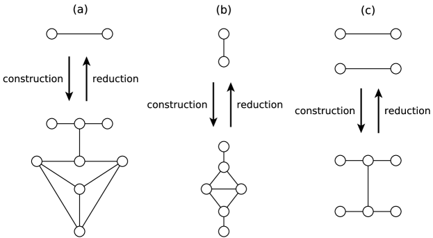
Figure 6: The construction operations for cubic graphs by de Vries [11, 12]. Note: the edge-pair to which operation $(c)$ is applied is allowed to have a common vertex.

Recall from Section 2.2 that $d_{e}(e_{1},e_{2})$ denotes the edge-distance between two edges $e_{1}$ and $e_{2}$. We define the minimum distance $d_{q}(e_{1},e_{2},e_{3},e_{4})$ of an edge-quadruple $\{\{e_{1},e_{2}\},\{e_{3},e_{4}\}\}$ as:

$$min[d(e_{1},e_{2}),d(e_{3},e_{4}),d(e_{1},e_{3})+1,d(e_{1},e_{4})+1,d(e_{2},e_{3})+1,d(e_{2},e_{4})+1]$$

From the definition of the $\mathcal{H}$ expansion we immediately get the following lemma:

Lemma 8.

When applying the $\mathcal{H}$ expansion operation to the edge-quadruple $\{\{e_{1},e_{2}\},\{e_{3},e_{4}\}\}$ without duplicate edges of a graph $G$, the smallest cycle in the expanded graph which contains an edge of the newly inserted $\mathcal{H}$ has size $d_{q}(e_{1},e_{2},e_{3},e_{4})+2$.

Theorem 9.

Every connected cubic graph $G$ with girth at least $k\geq 5$ has a reducible $\mathcal{H}$. The girth of the reduced graph is at least $k-2$ if $k\in\{5,6\}$ and at least $k-1$ otherwise.

Proof.

Let $e=\{v,w\}$ be a good edge in $G$ and $v_{1},v_{2},v_{3},v_{4}$ the vertices of the $\mathcal{H}$ not contained in $e$, so that in $\mathcal{H}$ we have that $d_{\mathcal{H}}(v_{1},v_{2})=d_{\mathcal{H}}(v_{3},v_{4})=2$. (Here $d_{G}(a,b)$ stands for the distance between two vertices $a$ and $b$ in the graph $G$). It follows that in the graph $\bar{G}=G[V(G)-\{v,w\}]$, $d_{\bar{G}}(v_{1},v_{2})\geq k-2$, $d_{\bar{G}}(v_{3},v_{4})\geq k-2$, and for $x\in\{v_{1},v_{2}\},y\in\{v_{3},v_{4}\}$ we have $d_{\bar{G}}(x,y)\geq k-3$. As all these distances are at least $2$, this also implies that after the reduction the edges that formerly contained an endpoint of the $\mathcal{H}$ are pairwise different.

If a cycle in $G$ that does not contain edges of the $\mathcal{H}$ centered around $e$, has length $g$ and contains $i$ vertices from $\{v_{1},v_{2},v_{3},v_{4}\}$, after the reduction it will have length $g-i$, so we have to prove that for each such cycle $g-i\geq k-2\geq 3$ to show that the result has neither loops nor double edges. Furthermore we have to show that for $k>6$ we have that $g-i\geq k-1$.

As $g\geq 5$ the result is trivial for $i=1$ for all $k$ and for $i\leq 2$ if $k\in\{5,6\}$. So assume just that $k>6$ and $i=2$. The distance of the two endpoints of the $\mathcal{H}$ on the cycle must be at least $k-3$, so $g\geq 2(k-3)=k+(k-6)\geq k+1$. So $g-i=g-2\geq k-1$.

So now assume that $k\geq 5$ and $i>2$.

If $i=3$, two of the vertices on the cycle come from one of the sets $\{v_{1},v_{2}\},\{v_{3},v_{4}\}$, so w.l.o.g. the vertices are $v_{1},v_{2},v_{3}$. This implies that $g\geq d_{\bar{G}}(v_{1},v_{2})+d_{\bar{G}}(v_{1},v_{3})+d_{\bar{G}}(v_{2},v_{3})\geq(k-2)+2(k-3)=k+(2k-8)\geq k+2$. So $g-i=g-3\geq k-1$.

If $i=4$ we have all $4$ vertices on the cycle and as $d_{\bar{G}}(x,y)\geq 2$ for all $x,y\in\{v_{1},v_{2},v_{3},v_{4}\}$, $x\not=y$, we have $g\geq 4(k-2)=k+(3k-8)\geq k+7$ and $g-i=g-4\geq k+3$.

∎

So all connected cubic graphs with girth at least $k$ (for $k\geq 5$) with $n$ vertices can be obtained by applying the $\mathcal{H}$ operation to all possible edge-quadruples of connected cubic graphs with $n-6$ vertices in such a way that the $\mathcal{H}$ operation destroys all cycles of size smaller than $k$ without creating any new cycles of size smaller than $k$. We call such edge-quadruples eligible edge-quadruples.

So in order for $\{\{e_{1},e_{2}\},\{e_{3},e_{4}\}\}$ to be an eligible edge-quadruple for generating cubic graphs with girth at least $k$, $d_{q}(e_{1},e_{2},e_{3},e_{4})$ must be at least $k-2$.

Assume our aim is to generate cubic graphs with girth at least $k$. We define the deficit $d(k,C)$ of a cycle $C$ in a graph $G$ as $max(k-|C|,0)$. We define the deficit $d(k,G)$ of a graph $G$ as:

$$max(\{\sum_{c\in C}d(k,c)\ |\ C\ \text{is a set of disjoint cycles of }G\})$$

Lemma 10.

When applying the $\mathcal{H}$ reduction operation to a cubic graph with girth at least $k\geq 5$, the reduced graph $G$ has deficit $d(k,G)\leq 4$.

Proof.

The fact that in a cycle of length $k-i$ at least $i$ edges must be intersected by endpoints of the $\mathcal{H}$ operation immediately implies that $d(k,G)\leq 4$.

∎

As in Section 2.2, we also use the canonical construction path method [23] to make sure that our algorithm does not output any isomorphic copies. The two rules of the canonical construction path method applied to the $\mathcal{H}$ operation algorithm are:

1. Only accept a cubic graph with girth at least $k$ if it was constructed by a canonical $\mathcal{H}$ expansion.

2. For every graph $G$ to which construction operations are applied, only perform one $\mathcal{H}$ expansion from each equivalence class of expansions of $G$.

Two edge-quadruples $\{\{e_{1},e_{2}\},\{e_{3},e_{4}\}\}$ and $\{\{e_{1}^{\prime},e_{2}^{\prime}\},\{e_{3}^{\prime},e_{4}^{\prime}\}\}$ of $G$ are called equivalent if there is an automorphism of $G$ mapping the set $\{\{e_{1},e_{2}\},\{e_{3},e_{4}\}\}$ to the set $\{\{e_{1}^{\prime},e_{2}^{\prime}\},\{e_{3}^{\prime},e_{4}^{\prime}\}\}$.

To define an efficient criterion for an $\mathcal{H}$ reduction of a graph $G$ to be canonical, we assign a $7$-tuple $(x_{0},\dots,x_{6})$ to the central edge $e_{c}$ of every reducible $\mathcal{H}$ and define a reducible $\mathcal{H}$ with the smallest $7$-tuple as the canonical reduction.

We did not implement the $\mathcal{H}$ operation for $k=5$ as then the edge-quadruples might contain incident edges, which would result in a large number of possibly eligible edge-quadruples, so that we did not expect an advantage over the tripod operation.

The values of $x_{0},\ldots,x_{4}$ are combinatorial invariants of increasing discriminating power and cost and are defined as follows:

1. $x_{0}$ is the number of hexagons containing $e_{c}$.

2. $x_{1}$ is the number of neighbours of $e_{c}$ which are part of a hexagon which does not contain $e_{c}$.

3. $x_{2}$ is the number of heptagons containing $e_{c}$.

4. $x_{3}$ is the number of vertices at distance at most $3$ from a vertex in $e_{c}$.

5. $x_{4}$ is the number of vertices at distance at most $4$ from a vertex in $e_{c}$.

Clearly, $x_{0}$ and $x_{1}$ are constant when generating graphs with girth at least $7$, so in that case they do not have to be computed.

Only if there are multiple reducible $\mathcal{H}$’s with the smallest value of $(x_{0},...,x_{4})$ (and the inserted $\mathcal{H}$ is one of them), we use nauty [22, 25] to compute a canonical labeling. The canonical vertex labeling induces a lexicographic ordering of the edges and we define $x_{5},x_{6}$ with $x_{5}<x_{6}$ to be the labels of the lexicographically smallest edge in the same orbit of $\operatorname{Aut}(G)$ as $e_{c}$.

The discriminating power of $(x_{0},...,x_{4})$ is usually enough to decide whether or not the reduction is canonical so the more expensive computation of $x_{5},x_{6}$ can often be avoided. For example for generating connected cubic graphs with girth at least $6$ and $34$ vertices, the computation of $x_{5},x_{6}$ is only required in about $3$% of the cases.

Also note that the definitions of $x_{0}$ or $x_{2}$ allow look-aheads on level $n-6$ for deciding whether or not an expansion can be canonical before actually performing the $\mathcal{H}$ expansion operation. For example for generating connected cubic graphs with girth at least $6$ and $34$ vertices, these look-aheads allow to avoid the construction of about $85$% of the graphs.

We omit the proof of the following theorem as it is completely analogous to the proof of Theorem 3.

Theorem 11.

Assume that exactly one representative $G$ of each isomorphism class of connected cubic graphs with $n-6$ vertices with deficit $d(k,G)$ at most 4 and girth at least $k-2$ (in case of $k\in\{5,6\}$) or girth at least $k-1$ (in case of $k\geq 7)$ is given. If we apply the following steps:

1. Apply the $\mathcal{H}$ insertion operation to one edge-quadruple in every equivalence class of eligible edge-quadruples.

2. Accept each graph with $n$ vertices if and only if the inserted $\mathcal{H}$ has minimal value of $(x_{0},\dots,x_{6})$ among all possible $\mathcal{H}$ reductions of the graph.

Then exactly one representative of each isomorphism class of connected cubic graphs with $n$ vertices and girth at least $k$ is accepted.

2.3.2 $\mathcal{H}$ operation for generating snarks

Similar to the tripod operation, also the $\mathcal{H}$ operation allows a look-ahead which often allows to avoid the generation of $3$-edge-colourable graphs with girth at least $k$.

Definition 12.

Let $\{\{e_{1},e_{2}\},\{e_{3},e_{4}\}\}$ be an edge-quadruple in a $3$-edge-coloured cubic graph and $\{c_{1},c_{2},c_{3}\}=\{1,2,3\}$.

A $(c_{1},c_{2})$-path from $e_{1}$ to $e_{3}$ together with an edge-disjoint $(c_{1},c_{3})$-path from $e_{2}$ to $e_{4}$ is called a prune-pair for $\{\{e_{1},e_{2}\},\{e_{3},e_{4}\}\}$.

Theorem 13.

Given a cubic graph $G$ and a $3$-edge-colouring $c$ of $G$. If there is a prune-pair for an edge-quadruple $\{\{e_{1},e_{2}\},\{e_{3},e_{4}\}\}$, then the graph obtained by extending $\{\{e_{1},e_{2}\},\{e_{3},e_{4}\}\}$ is $3$-edge-colourable.

Proof.

Suppose we apply the $\mathcal{H}$ expansion operation to $\{\{e_{1},e_{2}\},\{e_{3},e_{4}\}\}$ and call the obtained graph $G^{\prime}$. We can obtain a proper $3$-edge-colouring $c^{\prime}$ of $G^{\prime}$ by first starting from the colouring $c$ of $G$ and performing a Kempe-chain-like colour interchange of colours along the two paths of the prune-pair (see Figure 7).

Finally we colour the edges of the inserted $\mathcal{H}$ which are connected to $e_{1}$ and $e_{3}$ with the colour not present in the path connecting them, and analogously with $e_{2}$ and $e_{4}$. The central edge can then be coloured with the colour that occurred in both paths. The result is a proper $3$-edge-colouring of $G^{\prime}$.

∎

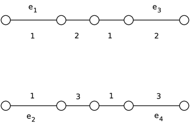
(a)

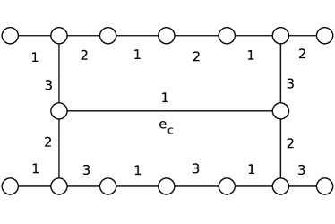
(b)

Figure 7: Procedure to recolour a graph after applying the $\mathcal{H}$ insertion operation to the edge-quadruple $\{\{e_{1},e_{2}\},\{e_{3},e_{4}\}\}$ used in the proof of Theorem 13.

We apply this look-ahead as follows for generating snarks with $n$ vertices and girth at least $k$. When a cubic graph $G$ with $n-6$ vertices is generated, we test if it is $3$-edge-colourable. If it is, we remove all edge-quadruples which can be discarded due to Theorem 13. This allows to discard about $47$% of the edge-quadruples which would otherwise be expanded for $k=6$ and $n=36$. We then also compute up to five additional colourings (as long as there are enough eligible edge-quadruples) and do the same. These five additional colourings raise the total percentage of discarded edge-quadruples to about $93$% for $k=6$ and $n=36$.

The cost for computing a seventh colouring turned out to be higher than the gain achieved by the additionally discarded edge-quadruples.

3 Results

3.1 Number of cubic graphs and running times

We implemented the tripod algorithm from Section 2.2 for generating connected cubic graphs with girth at least $k$ for $k=5,6$ and $7$ and the $\mathcal{H}$ algorithm from Section 2.3 for $k=6$ and $7$.

We will refer to our implementation of the tripod algorithm as snarkhunter-tripod and to our implementation of the $\mathcal{H}$ algorithm as snarkhunter-H, since we incorporated it in the existing generator for cubic graphs from [6] called snarkhunter.

In Tables 1-3 we give the counts of connected cubic graphs with girth at least $k$ and compare our new generators with the fastest existing generators for cubic graphs, i.e.: minibaum (which was developed by the first author [2]), genreg (which was developed by Meringer [26]) and snarkhunter (which we developed jointly with McKay [6]). Snarkhunter was only designed for $k\in\{3,4,5\}$. To make the distinction between this generator and snarkhunter-tripod and snarkhunter-h, we will refer to it as snarkhunter-old.

All running times reported in Tables 1-3 were obtained by executing the generators on an Intel Xeon CPU E5-268 CPU at 2.50GHz and include writing the generated graphs to a null device. The running times bigger than 3600 seconds include a small overhead due to parallelisation.

As can be seen from Table 1, snarkhunter-tripod is significantly faster than minibaum and genreg for generating cubic graphs with girth at least $5$, and is also faster – though not by such a large factor – than snarkhunter-old.

As can be seen from Table 2, both snarkhunter-tripod and snarkhunter-h are about 30 times faster than minibaum and genreg for generating cubic graphs with girth at least $6$ and $34$ vertices and the speedup seems to be increasing. For large orders, snarkhunter-h is a bit faster than snarkhunter-tripod.

As can be seen from Table 3, both snarkhunter-tripod and snarkhunter-h are a lot faster than minibaum and genreg for generating cubic graphs with girth at least $7$ and the speedup seems to be increasing very fast. For all orders which are within reach of the algorithm, snarkhunter-h is significantly faster than snarkhunter-tripod.

Our algorithms would also work for larger lower bounds $k$ on the girth, but they are likely to become less efficient for practical purposes for very large $k$. Note that for small vertex numbers and $k\leq 7$ the number of cubic graphs with girth at least $k$ grows a lot faster than the number of cubic graphs with girth at least $k-1$ (see e.g. Tables 1-3). As the algorithms described in this paper construct cubic graphs with girth at least $k$ from smaller cubic graphs with girth at least $k-1$, the running times of our generators grow a lot slower than the running times of generators such as genreg and minibaum. So for every $k$, the tripod algorithm or $\mathcal{H}$ algorithm will most likely become faster than genreg and minibaum for generating cubic graphs with girth at least $k$ from a certain number of vertices on. However we estimate that already for $k=8$ the point where our algorithms will become faster than genreg and minibaum will most likely not be within the range which is currently computationally feasible.

Tripod extension and $\mathcal{H}$ extension can be seen as the insertion of small trees. For larger girth it might be useful to insert larger trees, but this will go together with a serious increase of complexity of the algorithms.

In each case where a speedup is reported in Tables 1-3, this means that these graph counts have been independently confirmed by the corresponding generators. Since all results were in complete agreement, we believe that this provides strong evidence for the correctness of our implementations and results.

Order	# graphs	growth	sh-tripod (s)	mb (s) /	gr (s) /	sh-old (s) /
				sh-tripod (s)	sh-tripod (s)	sh-tripod (s)
22	90 938		0.7	8.14	7.33	1.57
24	1 620 479	17.82	10.3	9.22	9.36	1.75
26	31 478 584	19.43	195.3	9.26	10.44	1.67
28	656 783 890	20.86	4 538	8.29	10.53	1.51
30	14 621 871 204	22.26	117 048	7.43	9.53	1.43
32	345 975 648 562	23.66	2 797 926			1.35

Table 1: Counts and generation times for connected cubic graphs with girth at least 5. Sh-tripod stands for snarkhunter-tripod, mb for minibaum, gr for genreg and sh-old for snarkhunter-old.

Order	# graphs	growth	sh-h (s)	mb (s) /	gr (s) /	sh-tripod (s) /
				sh-h (s)	sh-h (s)	sh-h (s)
24	7 574		0.2	16.00	10.30	1.00
26	181 227	23.93	3.4	20.21	13.41	1.00
28	4 624 501	25.52	64	25.30	17.17	1.03
30	122 090 544	26.40	1 528.5	31.53	18.71	1.06
32	3 328 929 954	27.27	36 579	33.21	22.86	1.08
34	93 990 692 595	28.23	862 375	34.86	31.78	1.18
36	2 754 222 605 376	29.30	22 403 689			1.30

Table 2: Counts and generation times for connected cubic graphs with girth at least 6. Sh-h stands for snarkhunter-h, sh-tripod stands for snarkhunter-tripod, mb for minibaum and gr for genreg.

Order	# graphs	growth	sh-h (s)	mb (s) /	gr (s) /	sh-tripod (s) /
				sh-h (s)	sh-h (s)	sh-h (s)
30	546		0.4	17.00	7.03	11.00
32	30 368	55.62	7	38.61	10.48	11.03
34	1 782 840	58.71	186.1	83.68	20.25	9.02
36	95 079 083	53.33	6 968	126.95	26.94	7.41
38	4 686 063 120	49.29	214 412		43.76	5.33
40	220 323 447 962	47.02	7 049 445			4.72
42	10 090 653 722 861	45.80	383 939 689

Table 3: Counts and generation times for connected cubic graphs with girth at least $7$. Sh-h stands for snarkhunter-h, sh-tripod stands for snarkhunter-tripod, mb for minibaum and gr for genreg.

We incorporated the tripod and $\mathcal{H}$ algorithm into snarkhunter-old such that this program can now be used to generate all connected cubic graphs with girth at least $k$ for $3\leq k\leq 7$. The latest version of this generator can be downloaded from [4]. Several of the lists of cubic graphs from Tables 1-3 can be downloaded from the House of Graphs [3] at http://hog.grinvin.org/Cubic .

3.2 New lists of snarks and their properties

3.2.1 Numbers of snarks

We also incorporated the look-aheads described in Section 2 into the tripod and $\mathcal{H}$ algorithm so that snarks with girth at least $k$ can be generated more efficiently. This is significantly faster than just generating all cubic graphs with girth at least $k$ and applying a filter for colourability at the end (which was for $k>5$ up until now the only way to generate complete lists of snarks with girth at least $k$).

More specifically, for the tripod algorithm this is about $2$ times faster than the filter approach for $k=5$ and about $1.5$ times faster than the filter approach for $k=6$. For the $\mathcal{H}$ algorithm this is about $2$ times faster than the filter approach for $k=6$ and about $20$% faster than the filter approach for $k=7$. For higher girth there is more time required for generating a graph, so here the ratio for testing if a graph is colourable is smaller.

The numbers of snarks are shown in Table 4. Previously the complete list of all snarks up to $36$ vertices was known and it was also known that there are no snarks with girth at least $7$ up to at least 38 vertices.

Using the new algorithms we were able to generate all snarks with girth at least $6$ up to $38$ vertices. This took about $15$ CPU years.

As already mentioned in Section 1, the smallest snark with girth $7$ is currently unknown. Using the new algorithms we generated all snarks with girth at least $7$ up to $42$ vertices (which took about $12$ CPU years). As this did not yield any snarks, this shows that the smallest snark of girth $7$ must have at least $44$ vertices.

The tripod algorithm is faster than snarkhunter-old for generating snarks (i.e. girth at least $5$), but as the number of snarks grows very fast, it is still computationally infeasible to generate all snarks with $38$ vertices. However we did generate a sample of snarks with $38$ vertices and a sample of snarks with girth at least $6$ with $40$ vertices. These numbers are indicated with a ’$\geq$’ in Table 4. We estimate that it would take about $450$ CPU years to generate all snarks with girth at least $6$ with $40$ vertices on the computers used here.

We used the tripod algorithm to generate all snarks up to $34$ vertices and this confirmed the results in [5].

The complete list of snarks with girth at least $6$ and $38$ vertices were independently obtained by the tripod and $\mathcal{H}$ algorithm. However, as there are only $39$ such graphs, this does not provide very strong evidence for the correctness of these programs. Therefore we actually generated all connected cubic graphs with girth at least $6$ which are not $3$-edge-colourable (so not just the cyclically $4$-edge-connected ones). Both algorithms yielded the same $26~{}365$ graphs.

Also both the tripod algorithm and the $\mathcal{H}$ algorithm independently confirmed that there are no snarks with girth at least $7$ up to $40$ vertices. The computation for $42$ vertices was only performed using the $\mathcal{H}$ algorithm. Since all results were in complete agreement, we believe that this provides strong evidence for the correctness of our implementations and results.

All snarks from Table 4 can be downloaded from the House of Graphs [3] at http://hog.grinvin.org/Snarks . The adjacency lists from the snarks with $38$ vertices and girth $6$ can be inspected in the database of interesting graphs at the House of Graphs by searching for the keywords “snark * girth 6”.

Order	# snarks	$g\geq 6$	$g\geq 7$	$\lambda_{c}\geq 5$	$\lambda_{c}\geq 5$ and $g\geq 6$	$\lambda_{c}\geq 6$
10	1	0	0	1	0	0
12,14,16	0	0	0	0	0	0
18	2	0	0	0	0	0
20	6	0	0	1	0	0
22	20	0	0	2	0	0
24	38	0	0	2	0	0
26	280	0	0	10	0	0
28	2 900	1	0	75	1	1
30	28 399	1	0	509	1	0
32	293 059	0	0	2 953	0	0
34	3 833 587	0	0	19 935	0	0
36	60 167 732	1	0	180 612	1	1
38	$\geq$ 19 775 768	39	0	$\geq$ 35 429	0	0
40	?	$\geq 25$	0	?	$\geq 0$	?
42	?	?	0	?	?	?

Table 4: The number of snarks. The columns with a header of the form $g\geq a$ contain the number of snarks with girth at least $a$ and those of the form $\lambda_{c}\geq b$ contain the number of snarks with cyclic edge-connectivity at least $b$.

3.2.2 Properties of the new snarks

In this section we present an analysis of the new lists of snarks. None of the snarks with girth at least $6$ and $38$ vertices is cyclically $5$-edge-connected.

The dot product operation which was originally introduced by Isaacs in [15] allows to construct infinitely many snarks. When this operation is applied to two snarks $G_{1}$ and $G_{2}$, the result is a snark with $|V(G_{1})|+|V(G_{2})|-2$ vertices.

We implemented a program which performs the dot product operation and applied it to the complete lists of snarks. This resulted in the following observations.

Observation 14.

All of the 39 snarks with girth 6 and 38 vertices can be obtained by applying the dot product to two copies of the flower snark $J_{5}$.

Observation 15.

There are no snarks with girth at least 6 and 40 or 42 vertices which can be obtained by applying the dot product to a pair of snarks.

Observation 16.

There are 4 snarks with girth at least 6 and 44 vertices which can be obtained by applying the dot product to a pair of snarks.

For 46 vertices, we applied the dot product to every pair of snarks $\{G_{1},G_{2}\}$ which results in a snark on 46 vertices, except for the pairs where a snark with 38 vertices is combined with the Petersen graph as not all snarks with 38 vertices are known.

Observation 17.

There are at least 876 snarks with girth at least 6 and 46 vertices which can be obtained by applying the dot product to a pair of snarks.

All of the snarks from Observation 16 and 17 were obtained by applying the dot product operation to pairs of snarks where the flower snark $J_{5}$ is one of the two snarks.

A graph $G$ is hypohamiltonian if $G$ is not hamiltonian but $G-v$ is hamiltonian for every vertex $v$ in $G$.

Observation 18.

There are exactly 29 hypohamiltonian snarks with girth at least 6 and 38 vertices.

In the remainder we report how we used our new lists of snarks to test several conjectures, but it did not yield any counterexamples. For more information about the conjectures, we refer to [5]. We tested these conjectures using independently tested programs which were already used in [5].

A dominating cycle is a cycle $C$ such that every edge in $G$ has an endpoint on $C$. Fleischner [13] made the following conjecture related to dominating cycles:

Conjecture 19 (Fleischner [13]).

Every snark has a dominating cycle.

Observation 20.

Conjecture 19 holds for all snarks with girth 6 with at most 38 vertices.

Recall that a $k$-factor of a graph $G$ is a spanning $k$-regular subgraph of $G$. The oddness of a bridgeless cubic graph is the minimum number of odd order components in any 2-factor of the graph. The oddness of a cubic graph provides a measure for how far a the graph is from being colourable, as a graph has oddness 0 if and only if it is colourable.

Together with Hägglund and Markström we determined in [5] that all snarks with at most 36 vertices have oddness 2 and asked for the smallest snark with oddness greater than 2 (i.e. Problem 2 in [5]). Recently Lukot’ka et al. [21] have constructed a snark with oddness 4 and 44 vertices and they conjectured that it is the smallest snark with oddness 4.

Observation 21.

All snarks with girth at least 6 and at most 38 vertices have oddness 2.

Next to oddness, another measure for how far a graph is from being colourable is the notion of strong snarks which was introduced by Jaeger in [16]. A snark $G$ is strong if for every edge $e$ of $G$ the application of the edge reduction operation from Figure 1 results in an uncolourable graph. Celmins [10] proved that a minimum counterexample to the cycle double cover conjecture must be a strong snark.

In [5] we determined with Hägglund and Markström that there are no strong snarks with less than 34 vertices, exactly 7 strong snarks with 34 vertices and 25 strong snarks with 36 vertices.

Observation 22.

None of the snarks with girth at least 6 and at most 38 vertices is strong.

We also applied the edge insertion operation from Figure 1 in all possible ways to the complete list of snarks with 36 vertices and then tested which of the resulting graphs were strong snarks. This yielded the following result.

Observation 23.

There are at least 298 strong snarks with 38 vertices.

One might speculate that this is the complete set of strong snarks with 38 vertices, since applying the same procedure to all snarks with 32 and 34 vertices yields all 7 and 25 snarks with 34 and 36 vertices, respectively.

These strong snarks can also be obtained from the database of interesting graphs at the House of Graphs by searching for the keywords “strong snark”.

The total chromatic number of a graph $G$ is the minimum number of colours required to colour $E(G)\cup V(G)$ such that adjacent vertices and edges have different colours and no vertex has the same colour as its incident edges. It is known [29] that for cubic graphs the total chromatic number is either 4 or 5.

Cavicchioli et al. asked for the smallest snark with total chromatic number 5 (if any) (i.e. Problem 5.1 in [9]). Jointly with Hägglund and Markström, we showed in [5] that every snark up to at least 36 vertices has total chromatic number 4.

Recently, Brinkmann, Preissmann and Sasaki [8] gave a construction which yields weak snarks with total chromatic number 5 for every even order $n\geq 40$. A weak snark is a cyclically 4-edge-connected cubic graph with chromatic index 4 and girth at least 4.

Observation 24.

All snarks with girth at least 6 and at most 38 vertices have total chromatic number 4.

In [17] Jaeger made the following conjecture which is known as the Petersen colouring conjecture (we refer to [17] for more details).

Conjecture 25 (Jaeger [17]).

If $G$ is a bridgeless cubic graph, one can colour the edges of $G$ using the edges of the Petersen graph as colours in such a way that any three mutually adjacent edges of $G$ are coloured by three edges that are mutually adjacent in the Petersen graph.

Observation 26.

Conjecture 25 holds for all snarks with girth 6 with at most 38 vertices.

We also verified that there are no counterexamples to the above mentioned conjectures among the samples of snarks with 38 vertices and the samples of snarks with girth 6 and 40 vertices which are indicated with a ’$\geq$’ in Table 4.

References

Appendix: Adjacency lists

This section contains the adjacency lists of the complete list of 39 snarks with girth 6 and 38 vertices. These graphs can also be found on the House of Graphs [3] at http://hog.grinvin.org/Snarks .

The graphs are represented in the following compact format. The vertices of a graph $G$ are numbered from $0$ to $|V(G)|-1$ and each entry corresponds to the adjacency list of a graph where for a given vertex $v$, only the neighbours of $v$ which have a larger label than $v$ are listed. So the first 3 numbers are the neighbours of vertex 0, followed by the neighbours of vertex 1 which have a higher label than 1, etc.

1. {4, 8, 30, 6, 9, 14, 4, 7, 31, 7, 8, 15, 5, 19, 20, 7, 10, 9, 11, 13, 30, 13, 31, 13, 14, 16, 15, 17, 18, 34, 28, 32, 22, 24, 23, 26, 25, 27, 23, 25, 32, 23, 35, 25, 36, 29, 36, 29, 35, 29, 34, 33, 33, 33, 37, 37, 37}

2. {4, 8, 30, 6, 9, 14, 4, 7, 31, 7, 8, 15, 5, 19, 20, 7, 10, 9, 11, 13, 30, 13, 31, 13, 14, 16, 15, 17, 18, 28, 28, 34, 22, 24, 26, 35, 27, 36, 23, 25, 32, 23, 27, 35, 25, 26, 36, 29, 29, 29, 33, 33, 33, 34, 37, 37, 37}

3. {4, 8, 16, 6, 9, 14, 4, 7, 18, 7, 8, 15, 20, 15, 22, 28, 7, 10, 9, 11, 13, 16, 13, 18, 13, 14, 21, 15, 17, 21, 25, 19, 24, 30, 21, 26, 32, 34, 29, 32, 35, 28, 33, 27, 29, 31, 34, 31, 36, 29, 31, 35, 33, 36, 37, 37, 37}

4. {4, 8, 20, 5, 9, 11, 7, 9, 12, 7, 17, 18, 5, 12, 17, 7, 11, 15, 9, 15, 16, 19, 22, 19, 13, 26, 34, 15, 18, 21, 17, 20, 19, 28, 23, 34, 24, 27, 30, 32, 25, 31, 28, 32, 31, 33, 29, 33, 29, 30, 35, 35, 36, 36, 37, 37, 37}

5. {4, 8, 10, 5, 9, 11, 7, 9, 22, 5, 7, 18, 5, 12, 7, 11, 20, 9, 15, 11, 13, 24, 28, 14, 19, 15, 17, 20, 27, 29, 32, 18, 27, 21, 21, 25, 21, 23, 29, 33, 34, 30, 35, 30, 34, 28, 33, 36, 31, 29, 31, 36, 33, 35, 37, 37, 37}

6. {4, 8, 10, 5, 9, 11, 7, 9, 22, 5, 7, 18, 5, 12, 7, 11, 20, 9, 15, 11, 13, 24, 28, 14, 19, 15, 17, 20, 17, 29, 34, 18, 21, 21, 25, 21, 26, 34, 25, 28, 30, 27, 31, 27, 30, 32, 32, 33, 31, 33, 35, 35, 36, 36, 37, 37, 37}

7. {4, 8, 10, 5, 9, 11, 7, 9, 22, 5, 7, 18, 5, 12, 7, 11, 20, 9, 15, 11, 13, 16, 28, 14, 19, 15, 17, 20, 32, 34, 18, 26, 21, 21, 25, 21, 23, 30, 28, 33, 29, 32, 35, 27, 29, 31, 34, 31, 36, 29, 31, 35, 33, 36, 37, 37, 37}

8. {4, 8, 10, 5, 9, 11, 7, 9, 22, 5, 7, 18, 5, 12, 7, 11, 20, 9, 15, 11, 13, 28, 34, 14, 19, 15, 17, 20, 24, 26, 32, 18, 24, 21, 21, 23, 21, 25, 26, 27, 34, 29, 29, 33, 30, 30, 33, 31, 32, 31, 35, 35, 36, 36, 37, 37, 37}

9. {8, 10, 18, 6, 9, 12, 7, 11, 32, 5, 7, 8, 17, 20, 32, 17, 34, 10, 35, 35, 36, 11, 36, 13, 13, 15, 34, 15, 15, 24, 26, 21, 23, 28, 23, 19, 30, 20, 29, 21, 26, 23, 31, 33, 25, 33, 28, 30, 27, 29, 31, 29, 31, 33, 37, 37, 37}

10. {4, 8, 10, 5, 9, 11, 7, 9, 16, 5, 7, 18, 5, 12, 7, 11, 20, 9, 15, 11, 13, 28, 34, 14, 19, 15, 17, 20, 26, 34, 18, 25, 21, 21, 22, 21, 23, 27, 29, 30, 25, 27, 31, 29, 30, 32, 32, 31, 33, 33, 35, 35, 36, 36, 37, 37, 37}

11. {4, 8, 14, 5, 9, 20, 4, 11, 15, 7, 8, 12, 21, 12, 22, 7, 10, 19, 15, 9, 11, 13, 14, 13, 13, 17, 17, 17, 19, 20, 24, 28, 34, 24, 27, 28, 35, 26, 29, 27, 33, 35, 30, 30, 33, 36, 31, 32, 31, 29, 36, 31, 33, 34, 37, 37, 37}

12. {4, 8, 14, 5, 9, 20, 4, 11, 15, 7, 8, 12, 21, 12, 22, 7, 10, 19, 15, 9, 11, 13, 14, 13, 13, 17, 17, 17, 19, 20, 21, 30, 34, 24, 27, 28, 25, 29, 28, 33, 35, 30, 36, 33, 36, 27, 29, 32, 31, 29, 31, 35, 33, 34, 37, 37, 37}

13. {4, 20, 28, 6, 9, 29, 12, 30, 34, 7, 8, 21, 5, 11, 21, 29, 7, 20, 26, 9, 28, 30, 13, 14, 26, 15, 34, 16, 18, 18, 22, 16, 23, 17, 19, 35, 22, 35, 36, 23, 36, 24, 24, 25, 25, 27, 32, 27, 32, 31, 31, 33, 33, 33, 37, 37, 37}

14. {4, 8, 14, 6, 9, 16, 4, 7, 15, 7, 8, 17, 32, 22, 26, 34, 7, 10, 9, 11, 13, 14, 13, 15, 13, 16, 33, 30, 30, 17, 19, 25, 33, 35, 24, 27, 21, 26, 32, 25, 36, 23, 28, 27, 36, 25, 34, 29, 29, 31, 35, 31, 31, 33, 37, 37, 37}

15. {4, 8, 14, 6, 9, 16, 4, 7, 15, 7, 8, 17, 20, 22, 24, 34, 7, 10, 9, 11, 13, 14, 13, 15, 13, 16, 18, 30, 30, 17, 32, 25, 28, 24, 27, 32, 21, 26, 23, 25, 23, 28, 35, 25, 29, 34, 29, 35, 36, 31, 33, 33, 36, 33, 37, 37, 37}

16. {4, 8, 20, 5, 9, 11, 7, 9, 12, 7, 17, 18, 5, 12, 17, 7, 11, 15, 9, 15, 16, 19, 24, 19, 21, 24, 28, 32, 15, 18, 22, 17, 20, 19, 23, 26, 34, 25, 28, 29, 34, 27, 27, 33, 30, 32, 30, 31, 31, 33, 35, 35, 36, 36, 37, 37, 37}

17. {4, 8, 20, 5, 9, 11, 7, 9, 12, 7, 17, 18, 5, 12, 17, 7, 11, 15, 9, 15, 13, 16, 19, 19, 24, 26, 28, 15, 18, 22, 17, 20, 19, 27, 28, 32, 34, 23, 29, 32, 35, 25, 30, 29, 33, 31, 36, 31, 35, 29, 31, 34, 33, 36, 37, 37, 37}

18. {4, 8, 20, 5, 9, 11, 7, 9, 12, 7, 17, 18, 5, 12, 17, 7, 11, 15, 9, 15, 13, 16, 19, 19, 24, 30, 34, 15, 18, 22, 17, 20, 19, 27, 24, 32, 34, 25, 31, 28, 32, 35, 29, 29, 33, 27, 30, 36, 28, 29, 31, 35, 33, 36, 37, 37, 37}

19. {4, 10, 30, 6, 9, 14, 4, 11, 31, 7, 8, 15, 18, 18, 22, 26, 7, 10, 31, 9, 30, 11, 13, 13, 13, 14, 16, 15, 17, 19, 20, 19, 22, 21, 28, 23, 24, 25, 34, 23, 27, 25, 35, 28, 29, 35, 29, 34, 36, 32, 33, 33, 33, 36, 37, 37, 37}

20. {4, 10, 30, 6, 9, 14, 4, 11, 31, 7, 8, 15, 18, 18, 24, 32, 7, 10, 31, 9, 30, 11, 13, 13, 13, 14, 16, 15, 17, 19, 20, 19, 22, 26, 25, 23, 34, 23, 25, 35, 23, 36, 25, 27, 29, 35, 29, 34, 29, 32, 36, 33, 33, 33, 37, 37, 37}

21. {4, 8, 16, 6, 9, 14, 4, 7, 32, 7, 8, 15, 5, 15, 18, 7, 10, 9, 11, 13, 16, 13, 32, 13, 14, 20, 15, 17, 24, 26, 23, 27, 30, 33, 34, 21, 33, 22, 31, 26, 28, 30, 35, 29, 34, 27, 29, 36, 27, 29, 35, 31, 36, 33, 37, 37, 37}

22. {4, 8, 16, 6, 9, 14, 4, 7, 32, 7, 8, 15, 5, 15, 18, 7, 10, 9, 11, 13, 16, 13, 32, 13, 14, 20, 15, 17, 19, 24, 19, 22, 26, 21, 28, 27, 33, 25, 34, 25, 26, 35, 25, 36, 27, 29, 31, 35, 31, 34, 31, 33, 36, 33, 37, 37, 37}

23. {4, 8, 16, 6, 9, 14, 4, 7, 32, 7, 8, 15, 5, 15, 18, 7, 10, 9, 11, 13, 16, 13, 32, 13, 14, 20, 15, 17, 19, 24, 19, 22, 23, 21, 30, 28, 34, 25, 34, 26, 29, 25, 35, 29, 27, 30, 28, 35, 31, 36, 33, 33, 36, 33, 37, 37, 37}

24. {4, 8, 16, 6, 9, 14, 4, 7, 32, 7, 8, 15, 5, 15, 18, 7, 10, 9, 11, 13, 16, 13, 32, 13, 14, 19, 15, 17, 19, 20, 22, 28, 23, 21, 24, 26, 28, 27, 34, 25, 34, 25, 35, 30, 27, 36, 29, 31, 31, 35, 33, 36, 33, 33, 37, 37, 37}

25. {4, 10, 34, 6, 9, 32, 4, 11, 35, 5, 7, 8, 15, 18, 36, 7, 10, 35, 9, 34, 11, 13, 13, 13, 17, 28, 15, 16, 22, 36, 21, 32, 23, 33, 19, 26, 20, 22, 21, 24, 23, 25, 29, 27, 28, 27, 29, 27, 30, 31, 31, 31, 33, 33, 37, 37, 37}

26. {4, 10, 14, 6, 9, 18, 4, 11, 15, 7, 8, 19, 24, 22, 24, 32, 7, 10, 15, 9, 14, 11, 13, 13, 13, 18, 20, 17, 17, 17, 28, 32, 19, 23, 30, 34, 25, 26, 34, 27, 29, 25, 27, 25, 28, 31, 31, 35, 30, 35, 33, 36, 33, 36, 37, 37, 37}

27. {4, 10, 14, 6, 9, 18, 4, 11, 15, 7, 8, 19, 24, 16, 22, 24, 7, 10, 15, 9, 14, 11, 13, 13, 13, 18, 20, 17, 17, 17, 26, 19, 23, 30, 34, 25, 26, 28, 27, 34, 29, 32, 25, 32, 31, 29, 31, 30, 35, 35, 33, 36, 33, 36, 37, 37, 37}

28. {4, 10, 14, 6, 9, 18, 4, 11, 15, 7, 8, 19, 5, 16, 24, 7, 10, 15, 9, 14, 11, 13, 13, 13, 18, 20, 17, 17, 17, 26, 19, 23, 25, 28, 29, 32, 34, 23, 28, 33, 30, 31, 35, 32, 35, 27, 29, 31, 36, 29, 31, 34, 33, 36, 37, 37, 37}

29. {4, 10, 14, 6, 9, 18, 4, 11, 15, 7, 8, 19, 5, 16, 24, 7, 10, 15, 9, 14, 11, 13, 13, 13, 18, 34, 17, 17, 17, 21, 19, 35, 22, 25, 34, 28, 30, 29, 32, 26, 30, 32, 29, 31, 31, 33, 27, 35, 28, 33, 29, 31, 36, 36, 37, 37, 37}

30. {4, 10, 14, 6, 9, 18, 4, 11, 15, 7, 8, 19, 5, 16, 28, 7, 10, 15, 9, 14, 11, 13, 13, 13, 18, 20, 17, 17, 17, 21, 19, 23, 22, 34, 26, 34, 30, 32, 25, 27, 25, 28, 30, 33, 31, 33, 29, 31, 29, 32, 35, 35, 36, 36, 37, 37, 37}

31. {4, 8, 14, 6, 9, 15, 4, 7, 20, 7, 8, 16, 5, 16, 18, 7, 10, 9, 11, 13, 14, 13, 20, 13, 15, 18, 19, 22, 28, 22, 26, 30, 21, 26, 32, 21, 23, 27, 25, 34, 25, 28, 35, 27, 29, 36, 29, 31, 33, 35, 33, 36, 33, 34, 37, 37, 37}

32. {4, 8, 14, 6, 9, 15, 4, 7, 20, 7, 8, 16, 5, 16, 18, 7, 10, 9, 11, 13, 14, 13, 20, 13, 15, 18, 19, 22, 17, 26, 34, 21, 24, 27, 21, 28, 23, 32, 25, 27, 26, 35, 28, 30, 29, 31, 29, 36, 33, 35, 33, 36, 33, 34, 37, 37, 37}

33. {4, 8, 14, 6, 9, 15, 4, 7, 20, 7, 8, 16, 5, 16, 18, 7, 10, 9, 11, 13, 14, 13, 20, 13, 15, 18, 19, 22, 17, 28, 34, 21, 26, 34, 21, 25, 24, 29, 25, 29, 30, 27, 31, 27, 30, 32, 32, 31, 33, 33, 35, 35, 36, 36, 37, 37, 37}

34. {4, 8, 14, 6, 9, 15, 4, 7, 32, 7, 8, 16, 5, 16, 18, 7, 10, 9, 11, 13, 14, 13, 32, 13, 15, 18, 19, 21, 17, 22, 24, 19, 20, 25, 34, 23, 34, 26, 30, 26, 29, 29, 31, 27, 28, 35, 31, 35, 30, 36, 36, 33, 33, 33, 37, 37, 37}

35. {4, 10, 14, 6, 9, 16, 4, 11, 20, 5, 7, 8, 5, 12, 7, 10, 15, 14, 22, 11, 19, 13, 13, 13, 16, 17, 17, 18, 17, 24, 26, 23, 30, 21, 24, 27, 34, 23, 32, 28, 29, 27, 29, 35, 27, 36, 29, 31, 33, 35, 33, 36, 33, 34, 37, 37, 37}

36. {4, 10, 14, 6, 9, 16, 4, 11, 20, 5, 7, 8, 5, 12, 7, 10, 15, 14, 22, 11, 21, 13, 13, 13, 16, 17, 17, 18, 17, 24, 30, 21, 26, 34, 23, 25, 25, 26, 35, 24, 29, 33, 27, 31, 31, 33, 29, 30, 32, 35, 36, 36, 33, 34, 37, 37, 37}

37. {4, 10, 14, 6, 9, 16, 4, 11, 20, 5, 7, 8, 5, 12, 7, 10, 15, 14, 22, 11, 32, 13, 13, 13, 16, 17, 17, 18, 17, 28, 34, 22, 26, 30, 25, 27, 25, 26, 32, 33, 31, 33, 34, 25, 28, 35, 29, 31, 36, 29, 36, 31, 35, 33, 37, 37, 37}

38. {4, 8, 10, 6, 9, 14, 4, 7, 11, 7, 8, 17, 15, 15, 20, 28, 7, 34, 9, 35, 13, 34, 13, 35, 13, 16, 36, 32, 36, 32, 18, 21, 19, 28, 24, 30, 22, 25, 23, 24, 23, 31, 26, 30, 26, 27, 27, 31, 29, 29, 29, 33, 33, 33, 37, 37, 37}

39. {4, 10, 34, 6, 9, 16, 4, 11, 35, 5, 7, 8, 15, 24, 36, 7, 10, 35, 9, 34, 11, 13, 13, 17, 19, 28, 32, 16, 22, 29, 20, 36, 17, 30, 21, 24, 31, 22, 31, 21, 26, 23, 25, 25, 30, 27, 27, 27, 29, 29, 32, 33, 33, 33, 37, 37, 37}

References

- [1] A.T. Balaban. Valence-isomerism of cyclopolyenes. Revue Roumaine de chimie, 11(9):1097–1116, 1966.
- [2] G. Brinkmann. Fast generation of cubic graphs. Journal of Graph Theory, 23(2):139–149, 1996.
- [3] G. Brinkmann, K. Coolsaet, J. Goedgebeur, and H. Mélot. House of Graphs: a database of interesting graphs. Discrete Applied Mathematics, 161(1-2):311–314, 2013. Available at http://hog.grinvin.org/.
- [4] G. Brinkmann and J. Goedgebeur. Homepage of snarkhunter: http://caagt.ugent.be/cubic/.
- [5] G. Brinkmann, J. Goedgebeur, J. Hägglund, and K. Markström. Generation and properties of snarks. Journal of Combinatorial Theory, Series B, 103(4):468–488, 2013.
- [6] G. Brinkmann, J. Goedgebeur, and B.D. McKay. Generation of cubic graphs. Discrete Mathematics and Theoretical Computer Science, 13(2):69–80, 2011.
- [7] G. Brinkmann, J. Goedgebeur, and N. Van Cleemput. The history of the generation of cubic graphs. International Journal of Chemical Modeling, 5:67–89, 2013.
- [8] G. Brinkmann, M. Preissmann, and D. Sasaki. Snarks with total chromatic number 5. Discrete Mathematics & Theoretical Computer Science, 17(1):369–382, 2015.
- [9] A. Cavicchioli, T.E. Murgolo, B. Ruini, and F. Spaggiari. Special classes of snarks. Acta Applicandae Mathematica, 76(1):57–88, 2003.
- [10] U. Celmins. Cubic graphs that do not have an edge 3-colouring. Dissertation Abstracts International Part B: Science and Engineering, 46(5), 1985.
- [11] J. de Vries. Over vlakke configuraties waarin elk punt met twee lijnen incident is. Mededeelingen der Koninklijke Akademie voor Wetenschappen, Afdeeling Natuurkunde, 3(6):382–407, 1889.
- [12] J. de Vries. Sur les configurations planes dont chaque point supporte deux droites. Rendiconti Circolo Matematico Palermo, 5:221–226, 1891.
- [13] H. Fleischner. Some blood, sweat, but no tears in Eulerian graph theory. Congressus Numerantium, 63:8–48, 1988.
- [14] A. Huck. Reducible configurations for the cycle double cover conjecture. Discrete Applied Mathematics, 99(1):71–90, 2000.
- [15] R. Isaacs. Infinite families of nontrivial trivalent graphs which are not Tait colorable. American Mathematical Monthly, 82(3):221–239, 1975.
- [16] F. Jaeger. A survey of the cycle double cover conjecture. North-Holland Mathematics Studies, 115:1–12, 1985.
- [17] F. Jaeger. Nowhere-zero flow problems. Selected topics in graph theory, 3:71–95, 1988.
- [18] F. Jaeger and T. Swart. Conjecture 1. In M. Deza and I. G. Rosenberg, editors, Combinatorics 79, Part II, Annals of Discrete Mathematics, volume 9, page 305, 1980.
- [19] M. Kochol. Snarks without small cycles. Journal of Combinatorial Theory, Series B, 67(1):34–47, 1996.
- [20] H.W. Kroto, J.R. Heath, S.C. O’Brien, R.F. Curl, and R.E. Smalley. : Buckminsterfullerene. Nature, 318(6042):162–163, 1985.
- [21] R. Lukot’ka, E. Máčajová, J. Mazák, and M. Škoviera. Small snarks with large oddness. The Electronic Journal of Combinatorics, 22(1):20, 2015.
- [22] B.D. McKay. nauty User’s Guide (Version 2.5). Technical Report TR-CS-90-02, Department of Computer Science, Australian National University. The latest version of the software is available at http://cs.anu.edu.au/~bdm/nauty.
- [23] B.D. McKay. Isomorph-free exhaustive generation. Journal of Algorithms, 26(2):306–324, 1998.
- [24] B.D. McKay, W. Myrvold, and J. Nadon. Fast backtracking principles applied to find new cages. 9th Annual ACM-SIAM Symposium on Discrete Algorithms, pages 188–191, 1998.
- [25] B.D. McKay and A. Piperno. Practical graph isomorphism, II. Journal of Symbolic Computation, 60:94–112, 2014.
- [26] M. Meringer. Fast generation of regular graphs and construction of cages. Journal of Graph Theory, 30(2):137–146, 1999.
- [27] R.W. Robinson and N.C. Wormald. Numbers of cubic graphs. Journal of Graph Theory, 7:463–467, 1983.
- [28] R.W. Robinson and N.C. Wormald. Almost all cubic graphs are hamiltonian. Random Structures & Algorithms, 3(2):117–125, 1992.
- [29] M. Rosenfeld. On the total coloring of certain graphs. Israel Journal of Mathematics, 9(3):396–402, 1971.