Effective interactions and prospects for a resolution
of the fundamental cosmological problems in the quantum gravity
A possible effective interaction in the quantum gravity is considered. The compensation equation for a spontaneous generation of this interaction is shown to have a non-trivial solution. Would be consequences of a possible existence of effective interactions in the gravity theory are discussed. An example of running gravitational coupling is presented, which corresponds to a description of effects, which nowadays are prescribed to a dark mater and to a dark energy.
PACS: 11.15.Tk; 04.60.Bc; 98.80.Jk
Keywords: effective anomalous interaction; running gravity coupling; dark matter; dark energy
1 An effective three-graviton interaction
Due to well-known problems of the dark matter and the dark energy numerous possibilities of modified gravity are considered (see, e.g. review [1] and recent work [2]). This approach assumes existence of new effective interactions of the gravitational field in addition to the fundamental Einstein-Hilbert Lagrangian.
In the present work we would discuss a possibility of anomalous gravitation interaction in terms of non-perturbative effects of the Einstein-Hilbert gravity. For the purpose we rely on the approach induced by N.N. Bogoliubov compensation principle [3, 4]. In works [5] - [12], this approach was applied to studies of a spontaneous generation of effective non-local interactions in renormalizable gauge theories. The approach is described in full in book [13]. In particular, papers [9, 10] deal with an application of the approach to the electro-weak interaction and a possibility of spontaneous generation of effective anomalous three-boson interaction of the form
| (1) | |||
where is the electro-weak coupling. Here is a form-factor, which guarantees effective interaction (1) acting in a limited region of the momentum space. This form-factor is uniquely defined by the compensation equation of Bogoliubov approach. The approach gives unique results for physical parameters, so we have none adjusting parameter in the scheme. Would-be existence of effective interaction (1) leads to important non-perturbative effects in the electro-weak interaction [9, 11, 14]. Note, that interaction (1) was considered for long time on phenomenological grounds [15, 16].
We would take interaction (1) as a leading hint for choosing of an effective interaction in the gravity theory. Considering links between vector non-abelian gauge theories and the gravity theory, one easily see that gauge field plays the same role as Riemann curvature tensor . Thus the anomalous interaction which is strictly analogous to interaction (1) is the following
| (2) | |||
Here is again some form-factor to be defined by a compensation equation. We introduce this equation in the first approximation in what follows. We define the Lorentz structure of the anomalous three-graviton vertex, being quite lengthy, by calculations with application of FORM. We also use the standard Feynmann rules for the quantum gravity [17, 18].
It is important to emphasize, that wouldbe interaction (2) violates both the spatial P-invariance and the temporal T-invariance. Thus it might influence qualitative features of the Universe evolution. In particular, a violation of the T-invariance is necessary for an origin of the baryon asymmetry of the Universe [19].
Now let us turn to the compensation equation, which firstly answers the most important question, if interaction (2) can be spontaneously generated, and secondly, in case of affirmative answer to the first question, provides form-factor .
We start with the standard Einstein-Hilbert Lagrangian and expression , describing gauge interactions of the Standard Model.
| (3) |
Then we apply to expression (2) the add-subtract procedure, which in details is explained in [13]
| (4) | |||
| (5) |
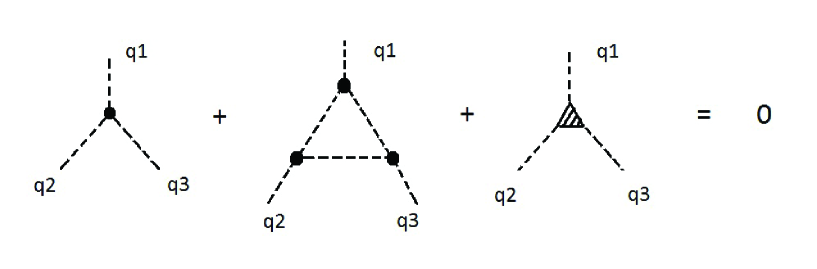
Now let us formulate the compensation equation. We are to demand, that considering the theory with Lagrangian (4), all contributions to three-graviton connected vertices, corresponding to Lorentz structure (2) are summed up to zero. That is the undesirable interaction part in the wouldbe free Lagrangian (4) is compensated. Then we are rested with interaction (2) only in the proper place (5). In a diagram form this demand in the first approximation is presented in Figure 1.
The corresponding integral equation with integrations in the Euclid momentum space is obtained also by FORM calculations and turns to be the following
| (6) | |||
where means an inhomogeneous part of the equation, which in Figure 1 is denoted by the striped triangle. We discuss the inhomogeneous part later on.
Assuming , by successive differentiations of equation (6) we obtain a linear differential equation for F(x), in which new variable is introduced
| (7) |
The differential equation is equivalent to equation (6) with boundary conditions. We have the following solution with an account of normalization condition
| (8) |
where is a Meijer function [20].
On the other hand, assuming , we may calculate from equation (6), that gives
| (9) |
However, form-factor has to be unity at zero. So there is evidently additional contribution to , that is
| (10) |
This contribution might be given by diagrams including matter fields, for example, by those being presented in Figure 2.
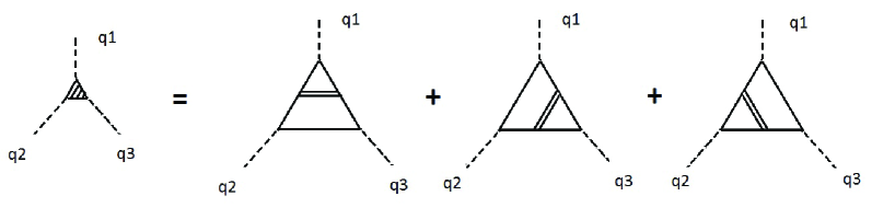
First of all we would draw attention to presence of exchange in Figure 2.
The contribution is provided by the the T-odd and P-odd part of fundamental fermions interaction with weak bosons . The interaction of with quarks and leptons contains matrix and so corresponding traces inevitably contains antisymmetric tensor , which is present in interaction (2). The vertex of a graviton interaction with a spinor field, is the following
where is the momentum of the incoming spinor, is the same of the outgoing one. is connected with the Planck mass
| (11) |
The -odd part of the quarks weak interaction is the following
| (12) |
where [21]
| (13) |
We readily estimate, that diagrams in Figure 2 with quark loops give the following contribution to the inhomogeneous part of the equation
| (14) |
where is the electro-weak gauge constant. As for lepton loops, we have no full information yet on corresponding mixing parameters, and thus we use for estimates only (14), the more so, as a quark loop has additional color factor 3. From the main equation (6) we have the following condition
| (15) |
Expression (14) has to be equal to
| (16) |
Then with previous relations (6, 16) we obtain the following estimate for the coupling constant of the effective interaction (2) . In doing this we have to bear in mind, that integral equation (6) is divided by coupling constant due to the overall procedure for searches for non-trivial solutions of compensation equations. Thus we have
| (17) |
As we have already mentioned, for the moment we can not substitute reliable values for the average neutrino mass and mixing parameters in analogous to (17) lepton expression. We may only safely assert, that is not zero due to existence of the effect of neutrino oscillations. In any case it may not be more than .
In view of this we have taken for the estimate just quarks, as particles giving contribution to coupling constant , the more so, as in the quark loops we have the additional color factor 3. It is evident, that massless particles, namely photons and gluons, do not give contribution due to parity conservation of their interactions. To obtain more definite connection between two parameters and one needs perform difficult calculations, which will be done elsewhere. However our estimate (17) allows us to consider qualitatively effects of the interaction (2).
With physical mass of and bearing in mind relation (11), where Planck mass is very large, we understand, that possible value (17) is essentially larger, than seemingly natural value , which one can estimate under premise, that only gravitational effects can define the quantity under the study.
The interaction (2) due to a presence of the antisymmetric tensor gives no contribution to spherically symmetric problems of gravitation (Schwartzschield solution, Friedmann solution etc.). However it could manifest itself in problems without spherical symmetry in a rotating system (e.g. spiral galaxy). The considerable enhancement of possible value in comparison to natural value by the following factor
| (18) |
is quite remarkable and presumably may lead to observable effects. Let us remind, that effective interaction (2) is and non-invariant.
2 A model for a running gravity coupling
We have considered above wouldbe properties of the quantum gravity. The theory itself contains dimensional coupling constant
| (19) |
In a conventional quantum field theory such quantity corresponds to a running coupling, for example, in QCD. Thus one should expect, that quantity (19) is also a running one. However, the quantum gravity theory is non-renormalizable. It means that we have no regular method to obtain an expression for the running coupling.
So an application of a non-perturbative approach is necessary. As a matter of fact, in gauge theories of the Standard Model contributions of the non-perturbative nature may be present also. We may refer just to the strong coupling , in which the well known non-physical Landau singularity appears in perturbative calculations. It is a general belief, that non-perturbative contributions somehow eliminate this singularity.
In particular, in work [12] we have shown, that the singularity is excluded due to the spontaneous generation of effective three-gluon interaction being analogous to (1). In any case, a consideration of possible properties of running gravitational coupling (19) deserves an attention. In the present section we consider a model, which illustrates the problem.
It is very important to have some hints on the scale of the possible non-perturbative effects in our problem. Here the example, which is considered in the previous Section may be instructive.
First of all, let us consider relation (18), which leads to the following estimate of characteristic length for effective interaction (2)
| (20) |
that is we have an essential enhancement of the characteristic length in comparison to the Planck one.
However effective interaction (2) is not the only possible one. Maybe there are also other effective interactions, which have even larger characteristic lengths. For example, we see, that in expression (17) both maximal mass parameter and masses of fundamental particles are present. Neutrino mass is the minimal one known. So we estimate a maximal possible scale of the length dimension for non-perturbative effects as follows
| (21) |
where we have used for the neutrino mass its upper bound [21]. We see, that this estimate gives a scale, which is appropriate to a size of a galaxy. Is it possible to use such scale for application to real astrophysical problems? In what follows we consider a hypothetical example of a gravity coupling behavior, which uses estimate (21).
Let us assume, that running Newton gravity coupling , which is proportional to coupling (19) depends on a distance in the following way
| (22) |
where is of the order the of magnitude of (21) and is just the well-known Newton constant. We use Meijer functions in the model, because in similar problems we encounter these functions. The Fourier transform of a Meijer function is again a Meijer function [22].

The gravity is not a logarithmic theory, as e.g. QCD, but a power-mode theory. We choose the coefficients in (22) so that for , and for . The last asymptotic corresponds to the accelerated expansion of the Universe, which usually is prescribed to a dark energy.
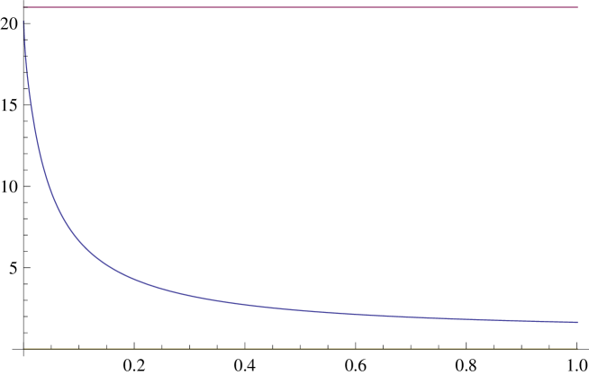
The Fourier transform, corresponding to expression (22), in a dependence on variable , where is a momentum, is the following [22]
| (23) |
Function (23) is shown in Figure 4. The momentum dependence resembles the situation with the asymptotic freedom in QCD. The main difference consists in a dependence at the infinity. In QCD the strong coupling decreases
| (24) |
while in the case under the consideration the gravity coupling tends to the Newton constant
| (25) |
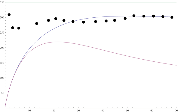
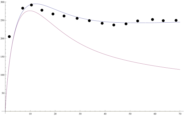
Now we apply representation (22) to rotation curves of galaxies. Let us choose . We take for a rotation curve of a flat disk galaxy the following expression
| (26) |
where is a galaxy mass in , is its radius in and r is a distance in a rotation curve in as well.
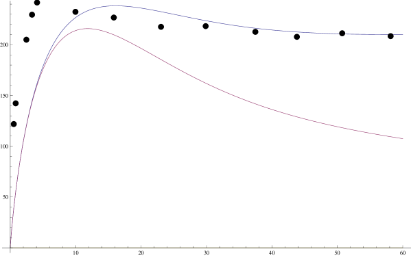
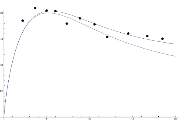
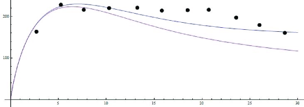
Then we substitute a galaxy mass and its radius to obtain a corresponding rotation curve. We have taken five galaxies for examples. Black spots in figures denote observation data, being taken from [23].
Upper curves in Figures correspond to
representation (26). All figures show how velocities in depend on distances in .
Lower curves in Figures correspond to , i.e. without
additional interaction. The examples show, that representation (22)
essentially improves the agreement with observational data.
Galaxy UGS 2885, , Figure 5.
Galaxy NGC 6674, , Figure 6.
Galaxy NGC 801, , Figure 7.
Galaxy NGC 3521, , Figure 8.
Galaxy NGC 2683, , Figure 9.
3 Conclusion
The present work deals with a possibility of a presence of effective interactions in
the gravity theory, the fundamental General Relativity. What are benefits of such possibility?
1. A wouldbe appearance of the P-odd and T-odd effective
interaction of gravitons with a new scale.
2. The toy model for dark effects, which with an assumption on a
special scale can pretend to a description of the real situation in
the astrophysics.
As for the last item, it is for the moment a hypothesis. It just show a possibility how things might be, in case searches for a dark matter and a proper understanding of the dark energy would fail. Note, that numerous proposals for a physical content of the dark substances also have a hypothetical status yet.
There are three regions in this model, in which properties of the gravitation turn to be quite different. In the first region the gravity coupling with the high accuracy equals the Newton one . In the region with this coupling increases, that leads to effects in the rotation curves, which usually are prescribed to a dark matter. Finally, in the region with is 21 times more, than the Newton coupling , that might serve as an explanation of the accelerated expansion of the Universe, which is nowadays usually prescribed to the dark energy. Thus, in case of such dependence of the gravity on a distance being realized, the presumptive effects of the dark matter and the dark energy are simultaneously described. Of course the present results are qualitative, a further specification is necessary for a more accurate comparison with data.
The purpose of the work is just to demonstrate a wouldbe tool to deal with effects in the gravity physics, which relies on close similarity of the gravity and vector non-abelian fields.
4 Acknowledgments
The work is supported in part by the Russian Ministry of Education and Science under grant NSh-3042.2014.2.
References
- [1] T.P. Sotiriou and V. Faraoni, Rev. Mod. Phys., 82, 451 (2010).
- [2] E.V. Arbuzova and A.D. Dolgov, Phys. Part. Nucl., 44, 204 (2013).
- [3] N.N. Bogoliubov. Soviet Phys.-Uspekhi, 67, 236 (1959).
- [4] N.N. Bogoliubov, Physica (Amsterdam), 26, S1 (1960).
- [5] B.A. Arbuzov, Theor. Math. Phys., 140, 1205 (2004);
- [6] B.A. Arbuzov, Phys. Atom. Nucl., 69, 1588 (2006).
- [7] B.A. Arbuzov, M.K. Volkov and I.V. Zaitsev, Int. J. Mod. Phys. A, 21, 5721 (2006).
- [8] B.A. Arbuzov, Phys. Lett. B, 656, 67 (2007).
- [9] B.A. Arbuzov, Eur. Phys. J. C, 61, 51 (2009).
- [10] B.A. Arbuzov and I.V. Zaitsev, Int. J. Mod. Phys. A, 26, 4945 (2011).
- [11] B.A. Arbuzov and I.V. Zaitsev, Phys. Rev. D 85: 093001 (2012).
- [12] B.A. Arbuzov and I.V. Zaitsev, Int. J. Mod. Phys. A, 28: 1350127 (2013).
- [13] B.A. Arbuzov, Non-perturbative Effective Interactions in the Standard Model, Walter De Gruyter GmbH, Berlin/Boston, 2014.
- [14] B.A. Arbuzov and I.V. Zaitsev, arXiv: 1510.02312 [hep-ph]; Int. J. Mod. Phys. A, to be published.
- [15] K. Hagiwara, R.D. Peccei, D. Zeppenfeld and K. Hikasa, Nucl. Phys. B, 282, 253 (1987).
- [16] K. Hagiwara, S. Ishihara, K. Szalapski and D. Zeppenfeld, Phys. Rev. D, 48, 2182 (1993).
- [17] B. DeWitt, Phys. Rev., 162, 1239 (1967).
- [18] L.D. Faddeev and V.N. Popov, Sov. Phys. Usp., 16, 777 (1974).
- [19] A.D. Sakharov, JETP, 51, 1059 (1980).
- [20] H. Bateman and A. Erdélyi, Higher transcendental functions, V. 1 Mc Graw-Hill, New York, Toronto, London, 1953.
- [21] K.A. Olive et al. (Particle Data Group), Chin.Phys., 38, 090001
- [22] A.P. Prudnikov, Yu.A. Brychkov, O.I. Marichev, Integrals and series, additional chapters, Nauka, Moscow, 1986, p. 350 (in Russian). (2014).
- [23] R.H. Sanders, Astrophys. J. 473, 117 (1996).