Two-loop calculation of anomalous kinetics of the reaction $A+A\rightarrow\varnothing$ in randomly stirred fluid

Abstract

The single-species annihilation reaction $\textit{A}+\textit{A}\rightarrow\varnothing$ is studied in the presence of a random velocity field generated by the stochastic Navier-Stokes equation. The renormalization group is used to analyze the combined influence of the density and velocity fluctuations on the long-time behavior of the system. The direct effect of velocity fluctuations on the reaction constant appears only from the two-loop order, therefore all stable fixed points of the renormalization group and their regions of stability are calculated in the two-loop approximation in the two-parameter $(\epsilon,\Delta)$ expansion. A renormalized integro-differential equation for the number density is put forward which takes into account the effect of density and velocity fluctuations at next-to-leading order. Solution of this equation in perturbation theory is calculated in a homogeneous system.

1 Introduction

The irreversible annihilation reaction $\textit{A}+\textit{A}\rightarrow\varnothing$ is a fundamental model of non-equilibrium physics. The reacting $A$ particles are assumed to perform chaotic motion due to diffusion or some external advection field such as atmospheric eddy and may react after the mutual collision with constant microscopic probability $K_{0}$ per unit time. Usually the resulting molecule is considered to be chemically inert with no backward influence on the movement of the reacting $A$ particles.

Many reactions of this type are observed in diverse chemical, biological or physical systems Derrida95 ; Kroon93 . The usual approach to such kind of problems is based on the use of the kinetic rate equation. It leads to a self-consistent description analogous to the mean-field approximation in the theory of critical phenomena. Its basic assumption is that the particle density is spatially homogeneous (fluctuations in concentration field are neglected). This homogeneity can be thought as a consequence of either an infinite mobility of the reactants or of a very small probability that a chemical reaction actually occurs when reacting entities meet each other. On the other hand, if the particle mobility becomes sufficiently small, or equivalently, if the microscopic reaction probability becomes large enough there is a possible transition to a new regime where it is more probable that the given particle reacts with local neighbors than with distant particles. This behavior is known as the diffusion-controlled regime Kampen ; Kang84 . For the annihilation reaction limited assumption of the density homogeneity leads to the following equation for the mean number density

$$\partial_{t}n(t)=-K_{0}n^{2}(t).$$ (1)

This equation predicts a long-time asymptotic decay as $n(t)\sim t^{-1}$ and the decay exponent does not depend on the space dimension. This is a common situation observed in the mean field theory. However, it turns out Lee94 ; Cardy96 that in lower space dimensions $d\leq 2$ the assumption of spatially uniform density, or equivalently of negligible density fluctuations of reacting particles, is not appropriate. Reentrant property of the diffusing particles Itzykson in low space dimensions leads to effective slowing-down of the reaction process and it can be rigorously shown, that the upper critical dimension for this process is $d_{c}=2$ Lee94 , above which the mean field approximation is valid.

A typical reaction occurs in liquid or gaseous environment. Thermal fluctuations of this underlying environment cause additional advection of the reacting particles. Therefore, it is interesting to study the influence of the advection field on the annihilation process.

Most of the renormalization-group analyses of the effect of random drift on the annihilation reaction $\textit{A}+\textit{A}\rightarrow\varnothing$ in the framework of the Doi approach have been carried out for the case of a quenched random drift field. Potential random drift with long-range Park ; Chung and short-range correlations Richardson99 have been studied as well as ”turbulent” flow (i.e. quenched solenoidal random field) with potential disorder Deem2 ; Tran . For a more realistic description of a turbulent flow time-dependent velocity field would be more appropriate. In Ref. Tran dynamic disorder with a given Gaussian distribution has been considered, whereas the most ambitious approach on the basis of a velocity field generated by the stochastic Navier-Stokes equation has been introduced here by two of the present authors Hnatic . From the point of the Navier-Stokes equation the situation near the critical dimension $d_{c}=2$ of the pure reaction model is even more intriguing due to the properties of the Navier-Stokes equation. It is well-known fact Frisch that in the case of space dimension $d=2$, there is inviscid conservation law of enstrophy absent in the three dimensional case. Calculations in Ref. Hnatic were performed in the one-loop approximation. As may readily seen from examination of the Feynman graphs, in the one-loop approximation there is no influence of the velocity fluctuations on the renormalization of the interaction vertices. However, the influence of higher order terms of the perturbation series can have significant effect on the critical properties. In this paper we study the advection of reactive scalar using random velocity field generated by the stochastic Navier-Stokes equation, which is used for production a velocity field corresponding to thermal fluctuations Forster1 ; Forster2 and a turbulent velocity field with the Kolmogorov scaling behavior Adzhemyan . It should be stressed, moreover, that in the presented model we assume that there is no influence of the reactant on the velocity field itself. Therefore, the model may be characterized as a model for the advection of a passive chemically active admixture.

A powerful tool for analyzing the asymptotic behavior of stochastic systems is provided by the renormalization-group (RG) method. It allows to determine the long-time and large-scale – or infra-red (IR) – asymptotic regimes of the system and also is very efficient tool for calculation of various universal physical quantities, e.g. critical exponents. The aim of this paper is to examine the IR behavior of the annihilation process under the influence of advecting velocity fluctuations and to determine its stability in the second order of the perturbation theory.

Using the mapping procedure based on the Doi formalism Doi1 ; Doi2 an effective field-theoretic model for the annihilation process is constructed. The RG method is applied to the model in the field-theoretic formulation, which is the most efficient in calculations beyond the one-loop order, and the renormalization constants and fixed points of the renormalization group are determined in the two-loop approximation within the two-parameter expansion. The non-linear integro-differential equation, which includes first non-trivial corrections to (1), is obtained for the mean number density and it is shown how the information about IR asymptotics can be extracted from it in the case of a homogeneous system. This equation allows to investigate heterogeneous systems as well as to take into account the effect of density and advecting velocity fluctuations. However, solution of the equation in the heterogenous case requires heavy numerical calculations and is beyond the scope of the present paper. We intend to return to this problem in future work.

The paper is organized as follows. In Sec. II the field-theoretic model for the annihilation process is constructed on the basis of the second-quantization approach. The basic ingredients for the modeling of a velocity field by the stochastic Navier-Stokes equation are presented. It is also shown how both the Kolmogorov scaling and thermal fluctuations can be included into the model. The ultraviolet (UV) renormalization of the model and the elaborated algorithm for the calculation of the renormalization constants is described in Sec. III. Fixed points of the RG are classified together with their stability regions and possible scaling regimes are presented in Sec IV. In Sec. V the integro-differential equation for the mean number density is derived and analysis of its solution is given. Conclusions are presented in Sec. VI.

2 Field-theoretic model of the annihilation reaction

Let us study anomalous kinetics of the generic type of the irreversible single-species annihilation reaction

$$A+A\xrightarrow{K_{0}}\varnothing,$$ (2)

with the unrenormalized (mean field) rate constant $K_{0}$. The first step of the Doi approach Doi1 ; Doi2 (see also Peliti ) consists of the introduction of the creation and annihilation operators $\psi^{\dagger}$ and $\psi$ and the vacuum state $|0\rangle$ satisfying the usual bosonic commutation relations

$$[\psi(\mathbf{x}),\psi^{\dagger}({\mathbf{x}^{\prime}})]=\delta(\mathbf{x}-{\mathbf{x}^{\prime}}),$$

$$[\psi(\mathbf{x}),\psi({\mathbf{x}^{\prime}})]=[\psi^{\dagger}(\mathbf{x}),\psi^{\dagger}(\mathbf{x^{\prime}})]=0,$$

$$\psi(\mathbf{x})|0\rangle=0,\langle 0|\psi^{\dagger}(\mathbf{x})=0,\langle 0|0\rangle=1.$$ (3)

Let $P(\{n_{i}\},t)$ be the joint probability density function (PDF) for observing $n_{i}$ particles at positions $\mathbf{x}_{i}$. The information about the macroscopic state of the classical many-particle system may be transferred into the state vector $|\Phi(t)\rangle$ defined as the sum over all occupation numbers

$$|\Phi(t)\rangle=\sum_{\{n_{i}\}}P(\{n_{i}\},t)|\{n_{i}\}\rangle,$$ (4)

where the basis vectors are defined as

$$|\{n_{i}\}\rangle=\prod_{i}[\psi^{\dagger}(\mathbf{x}_{i})]^{n_{i}}|0\rangle.$$ (5)

The whole set of coupled partial differential equations for the PDFs may be rewritten in the compact form of a master equation Lee94 ; Doi1 ; Doi2

$$\frac{\partial}{\partial t}|\Phi(t)\rangle=-\hat{H}|\Phi(t)\rangle,$$ (6)

where $\hat{H}=\hat{H}_{A}+\hat{H}_{D}+\hat{H}_{R}$ and for the annihilation process $A+A\rightarrow\varnothing$ under consideration

$$\hat{H}_{A}=\int d{\mathbf{x}}\mbox{ }\psi^{\dagger}\nabla[{\mathbf{v}}({\mathbf{x}},t)\psi({\mathbf{x}})],$$

$$\hat{H}_{D}=-D_{0}\int d{\mathbf{x}}\mbox{ }\psi^{\dagger}\nabla^{2}\psi({\mathbf{x}}),$$

$$\hat{H}_{R}=\lambda_{0}D_{0}\int d{\mathbf{x}}\mbox{ }(\psi^{\dagger})^{2}\psi^{2},$$ (7)

corresponding to the advection, diffusion and reaction parts of the operator $\hat{H}$ Hnatic . Due to dimensional reasons we have extracted the diffusion constant $D_{0}$ from the rate constant $K_{0}=\lambda_{0}D_{0}$.

The mean of an observable quantity $\mathcal{O}(t)$ may be expressed Hnatic as the vacuum expectation value

$$\langle\mathcal{O}(t)\rangle = \langle 0|T(\mathcal{O}\{[\psi^{\dagger}(t)+1]\psi(t)\}$$ (8)

$$\times {\rm e}^{-\int^{\infty}_{0}\hat{H}^{\prime}_{I}dt+n_{0}\int d{\mathbf{x}}\mbox{ }\psi^{\dagger}({\mathbf{x}},0)})|0\rangle.$$

Here, the interaction operator is defined as $\hat{H}^{\prime}_{I}=\hat{H}^{\prime}-\hat{H}^{\prime}_{0}$ and the substitution $\psi^{\dagger}\rightarrow\psi^{\dagger}+1:\hat{H}^{\prime}\equiv\hat{H}(\psi^{\dagger}+1,\psi)$ is understood. The field operators (3) are replaced by the time-dependent operators of the interaction representation

$$\psi^{\dagger}(t,{\mathbf{x}})={\mathrm{e}}^{\hat{H}_{0}^{\prime}t}\psi^{\dagger}({\mathbf{x}}){\mathrm{e}}^{-\hat{H}_{0}^{\prime}t},\quad\psi(t,{\mathbf{x}})={\mathrm{e}}^{\hat{H}_{0}^{\prime}t}\psi({\mathbf{x}}){\mathrm{e}}^{-\hat{H}_{0}^{\prime}t}.$$

In this formulation - assuming the Poisson distribution as the initial condition - the average number density can be computed via the expression

$$n(t,{\mathbf{x}})=\langle 0|\psi({\mathbf{x}}){\mathrm{e}}^{-\hat{H}^{\prime}t}{\mathrm{e}}^{n_{0}\int d{\mathbf{x}}\psi^{\dagger}}|0\rangle,$$ (9)

where $n_{0}$ is the initial number density. The expectation value of the time-ordered product in (8) can be cast Vasiliev into the form of a functional integral over scalar fields $\psi^{\dagger}(\mathbf{x},t)$ and $\psi(\mathbf{x},t)$:

$$\langle\mathcal{O}(t)\rangle=\int\mathcal{D}\psi^{\dagger}\mathcal{D}\psi\mbox{ }\mathcal{O}\{[\psi^{\dagger}(t)+1]\psi(t)\}\rm{e}^{S_{1}},$$ (10)

where the action $S_{1}$ for the annihilation reaction $\textit{A}+\textit{A}\rightarrow\varnothing$ is

$$S_{1} = -\int^{\infty}_{0}dt\int d{\mathbf{x}}\{\psi^{\dagger}\partial_{t}\psi+\psi^{\dagger}\nabla({\mathbf{v}}\psi)-D_{0}\psi^{\dagger}\nabla^{2}\psi$$ (11)

$$+ \lambda_{0}D_{0}[2\psi^{\dagger}+(\psi^{\dagger})^{2}]\psi^{2}\}+n_{0}\int d{\mathbf{x}}\mbox{ }\psi^{\dagger}({\mathbf{x}},0).$$

In order to analyze the effect of velocity fluctuations on the reaction process we average the expectation value (10) over the random velocity field $\mathbf{v}$. The most realistic description of the velocity field ${\bf v}$ is based on the use of the stochastic Navier-Stokes equation Adzhemyan . Due to the incompressibility conditions $\nabla\cdot\mathbf{v}=0$ and $\nabla\cdot\mathbf{f}^{v}=0$ imposed on the velocity field $\mathbf{v}$ and the random-force field $\mathbf{f}^{v}$ it is possible to eliminate pressure from the Navier-Stokes equation and hence it is sufficient to consider only its transverse components

$$\partial_{t}{\mathbf{v}}+P({\mathbf{v}}\cdot\nabla){\mathbf{v}}-\nu_{0}\nabla^{2}{\mathbf{v}}={\mathbf{f}}^{v}.$$ (12)

Here, $\nu_{0}$ is the molecular kinematic viscosity, $P_{ij}({\bf k})=\delta_{ij}-k_{i}k_{j}/k^{2}$ is the transverse projection operator and $k=|{\bf k}|$ is the norm of the wave vector ${\mathbf{k}}$. Here and below we use the subscript $"0"$ for all ”bare” parameters to distinguish them from their renormalized counterparts, which will appear during the renormalization procedure.

The large-scale random force per unit mass ${\mathbf{f}}$ is assumed to be a Gaussian random variable with zero mean and the following correlation function

$$\langle f_{m}({\mathbf{x}}_{1},t_{1})f_{n}({\mathbf{x}}_{2},t_{2})\rangle=\delta(t_{1}-t_{2})$$

$$\times\int\frac{d{\mathbf{k}}}{(2\pi)^{d}}P_{mn}({\mathbf{k}})d_{f}(k)\rm{e}^{i{\mathbf{k}}\cdot({\mathbf{x}}_{1}-{\mathbf{x}}_{2})},$$ (13)

where the kernel function is chosen in the form

$$d_{f}(k)=g_{10}\nu_{0}^{3}k^{4-d-2\epsilon}+g_{20}\nu_{0}^{3}k^{2}.$$ (14)

The nonlocal term is often used to generate the turbulent velocity field with Kolmogorov’s scaling Adzhemyan ; Dominicis ; Vasiliev04 . That case is achieved by setting $\epsilon=2$. The local term $g_{20}\nu_{0}^{3}k^{2}$ has been added not only because of renormalization reasons but has also an important physical meaning. Such a term in the force correlation function describes generation of thermal fluctuations of the velocity field near equilibrium Forster1 ; Forster2 and thus can mimic the usual environment in which chemical reactions take place.

Averaging in the expectation value (10) over the realizations of the random velocity field ${\mathbf{v}}$ is done with the use of the ”weight” functional $\mathcal{W}_{2}=\rm{e}^{S_{2}}$. Here, $S_{2}$ is the effective action for the advecting velocity field Vasiliev04

$$S_{2} = \frac{1}{2}\int dtd{\mathbf{x}}d{\mathbf{x}^{\prime}}\mbox{ }\tilde{\mathbf{v}}({\mathbf{x}},t)\cdot\tilde{{\mathbf{v}}}({\mathbf{x}}^{\prime},t)d_{f}(|{\mathbf{x}}-{\mathbf{x}}^{\prime}|)$$ (15)

$$+ \int dtd{\mathbf{x}}\mbox{ }\tilde{{\mathbf{v}}}\cdot[-\partial_{t}{\mathbf{v}}-({\mathbf{v}}\cdot\nabla){\mathbf{v}}+\nu_{0}\nabla^{2}{\mathbf{v}}],$$

where $\tilde{{\mathbf{v}}}$ is the auxiliary transverse vector field, that results from the Gaussian averaging with respect to the realizations of random force ${\mathbf{f}}^{v}$. The appearance of such field is common for the models of stochastic dynamics and the field itself can be understood as a response field Jan76 .

With the use of the complete weight functional

$$\mathcal{W}=\rm{e}^{S_{1}+S_{2}}$$ (16)

it is possible to evaluate the expectation value of any desirable physical observable.

Actions (11) and (15) for the studied model are written in the form convenient for the use of the standard Feynman diagrammatic technique.

Figure 1: The propagators of the model

The inverse matrix of the quadratic part of the actions determines the form of the bare propagators. In the Feynman graphs these propagators correspond to lines connecting interaction vertices. It is easily seen that the studied model contains three different types of propagators. The propagators are presented in the wave-number-frequency representation, which is the most convenient way for doing explicit calculations. The graphical representation of the propagators is presented in Fig. 1, where

$$\Delta_{ij}^{v\tilde{v}}(\omega_{k},{\mathbf{k}})=\frac{P_{ij}({\mathbf{k}})}{-i\omega_{k}+\nu_{0}k^{2}}\,,\Delta_{ij}^{vv}(\omega_{k},{\mathbf{k}})=\frac{d_{f}(k)P_{ij}^{k}({\mathbf{k}})}{\omega_{k}^{2}+\nu_{0}^{2}k^{4}},$$

$$\hskip 56.9055pt\Delta^{\psi\psi^{\dagger}}(\omega_{k},{\mathbf{k}})=\frac{1}{-i\omega_{k}+D_{0}k^{2}},$$ (17)

with the kernel function $d_{f}(k)$ given by the expression (14). The vertex factor

$$V_{m}(x_{1},x_{2},\ldots,x_{m};\Phi)=\frac{\delta^{m}V(\Phi)}{\delta\Phi(x_{1})\delta\Phi(x_{2})\ldots\delta\Phi(x_{m})}$$ (18)

is associated to each interaction vertex of Feynman graph. Here, $\Phi$ could be any member from the set of all fields $\{\psi^{\dagger},\psi,\tilde{v},v\}$. The interaction vertices from action (15) describe the advection of reactant particles by the velocity field and the interactions between the velocity components. The interaction vertex in (15) may be rewritten in a technically more convenient form

$$-\int dtd{\mathbf{x}}\mbox{ }\tilde{{\mathbf{v}}}({\mathbf{v}}\cdot\nabla){{\mathbf{v}}}=-\int dtd{\mathbf{x}}\mbox{ }\tilde{v}_{i}v_{k}\partial_{k}v_{i}$$

$$=\int dtd{\mathbf{x}}\mbox{ }(\partial_{k}\tilde{v}_{i})v_{k}v_{i},$$ (19)

where the incompressibility condition $\partial_{i}v_{i}=0$ and partial integration method have been used. We have assumed that the velocity fields fall off rapidly for $|\mathbf{x}|\rightarrow\infty$ and therefore the surface terms can be neglected. Rewriting (19) into the symmetric form $v_{i}V_{ijl}v_{j}v_{l}/2$, it is easy to find the explicit form for the corresponding vertex factor in the momentum space

$$V_{ijl}=i(k_{j}\delta_{il}+k_{l}\delta_{ij}).$$ (20)

Here, the momentum ${\mathbf{k}}$ is flowing into the vertex through the field $\tilde{v}$. The advecting term from the action (11) can be similarly modified as follows

$$-\int dtd{\mathbf{x}}\mbox{ }\psi^{\dagger}\nabla({\mathbf{v}}\psi)=-\int dtd{\mathbf{x}}\mbox{ }\psi^{\dagger}\partial_{i}(v_{i}\psi)$$

$$=-\int dtd{\mathbf{x}}\mbox{ }\psi^{\dagger}v_{i}\partial_{i}\psi=\int dtd{\mathbf{x}}\mbox{ }(\partial_{i}\psi^{\dagger})v_{i}\psi.$$ (21)

Rewriting this expression in the form $\psi^{\dagger}V_{j}v_{j}\psi$ we obtain immediately the vertex factor in the momentum space

$$V_{j}=ik_{j}.$$ (22)

The momentum ${\mathbf{k}}$ represents the momentum flowing into the diagram through the slashed field $\psi^{\dagger}$. These two vertices (20), (22) are depicted in Fig. 2.

Figure 2: Interaction vertices describing velocity fluctuation and advection and the corresponding vertex factors

The two reaction vertices derived from the functional (11) are depicted in Fig. 3 and physically describe the density fluctuations of the reactant particles. The vertex factors for both of them follows from the straightforward application of the definition (18).

Figure 3: Interaction vertices responsible for density fluctuations and their corresponding vertex factor

3 UV renormalization of the model

The functional formulation provides a theoretical framework suitable for applying methods of quantum field theory. Using RG methods it is possible to determine the IR asymptotic (large spatial and time scales) behavior of the correlation functions. First of all, a proper renormalization procedure is needed for the elimination of ultraviolet (UV) divergences. There are various renormalization prescriptions applicable for such a task, each with its own advantages. To most popular belong the Pauli-Villars, lattice and dimensional regularization Zinn-Justin89 . In what follows we will employ the modified minimal subtraction ($\overline{\text{MS}}$) scheme. Strictly speaking, in the analytic renormalization there is no consistent MS scheme. What we mean here, is the ray scheme Adzhemyan3 , in which the two regularizing parameters $\epsilon$, $\Delta$ ($\epsilon$ has been introduced in (14) and $2\Delta=d-2$) are taken proportional to each other: $\Delta=\xi\epsilon$, where the coefficient $\xi$ is arbitrary but fixed. In this case, only one independent small parameter, say, $\epsilon$ remains and the notion of minimal subtraction becomes meaningful. UV divergences manifest themselves in the form of poles in the small expansion parameter and the minimal subtraction scheme is characterized by discarding all finite parts of the Feynman graphs in the calculation of the renormalization constants. In the modified scheme, as usual, certain geometric factors are not expanded in $\epsilon$, however. This is the content of the $\overline{\text{MS}}$ scheme used in our analysis.

In order to apply the dimensional regularization for the evaluation of renormalization constants, an analysis of possible superficial divergences has to be performed. For the power counting in the actions (11) and (15) we use the scheme Adzhemyan , in which to each quantity $Q$ two canonical dimensions are assigned, one with respect to the wave number $d_{Q}^{k}$ and the other to the frequency $d_{Q}^{\omega}$. The normalization for these dimensions is

$$d^{\omega}_{\omega}=-d_{t}^{\omega}=1,\quad d_{k}^{k}=-d_{x}^{k}=1,\quad d_{k}^{\omega}=d^{k}_{\omega}=0.$$ (23)

The canonical (engineering) dimensions for fields and parameters of the model are derived from the condition for action to be a scale-invariant quantity, i.e. to have a zero canonical dimension. The quadratic part of the action (11) determines only the canonical dimension of the quadratic product $\psi^{\dagger}\psi$. In order to keep both terms in the nonlinear part of the action

$$\lambda_{0}D_{0}\int dtd\mathbf{x}[2\psi^{\dagger}+(\psi^{\dagger})^{2}]\psi^{2},$$ (24)

the field $\psi^{\dagger}$ must be dimensionless. If the field $\psi^{\dagger}$ has a positive canonical dimension, which is the case for $d>2$, then the quartic term should be discarded as irrelevant by the power counting. The action with the cubic term only, however, does not generate any loop integrals corresponding to the density fluctuations and thus is uninteresting for the analysis of fluctuation effects in the space dimension $d=2$.

Using the normalization choice (23), we are able to obtain the canonical dimensions for all the fields and parameters in the $d$-dimensional space. The results are summarized in Table 1.

Table 1: Canonical dimensions for the parameters and the fields of the model

1 $Q$	$\psi$	$\psi^{\dagger}$	$v$	$\tilde{v}$	$\nu_{0},D_{0}$	$\lambda_{0}$	$g_{10}$	$g_{20}$
$d_{Q}^{\omega}$	$0$	$0$	$1$	$-1$	$1$	$0$	$0$	$0$
$d_{Q}^{k}$	$d$	$0$	$-1$	$d+1$	$-2$	$-2\Delta$	$2\epsilon$	$-2\Delta$
$d_{Q}$	$d$	$0$	$1$	$d-1$	$0$	$-2\Delta$	$2\epsilon$	$-2\Delta$

Here, $d_{Q}=d^{k}_{Q}+2d_{Q}^{\omega}$ is the total canonical dimension and it is determined from the condition that the parabolic differential operator of the diffusion and Navier-Stokes equation scales uniformly under the simultaneous momentum and frequency dilatation $k\rightarrow\mu k,\omega\rightarrow\mu^{2}\omega$.

The model is logarithmic when canonical dimensions of all the coupling constants $\{g_{10},g_{20},\lambda_{0},u_{0}\}$ vanish simultaneously. From Table 1 it follows that this situation occurs for the choice $\epsilon=\Delta=0$. The parameter $\epsilon$ characterizes the deviation from the Kolmogorov scaling Adzhemyan99 observed in the real turbulence and together with $\Delta$ may be considered as the analog of the expansion parameter $\epsilon=4-d$ used in the theory of critical phenomena. The UV divergences have the form of poles in various linear combinations of $\epsilon$ and $\Delta$. The total canonical dimension of an arbitrary one-particle irreducible Green (1PI) function $\Gamma=\langle\Phi\ldots\Phi\rangle_{\rm 1-ir}$ is given by the relation $d_{\Gamma}=d+2-N_{\Phi}d_{\Phi},$ where $N_{\Phi}=\{N_{\psi^{\dagger}},N_{\psi},N_{v},N_{\tilde{v}}\}$ are the numbers of corresponding external fields entering into the function $\Gamma$.

The statistical averaging $\langle\ldots\rangle$ means averaging over all possible realizations of fields $\tilde{{\mathbf{v}}},{\mathbf{v}},\psi^{\dagger},\psi$ satisfying appropriate boundary conditions with the use of the complete weight functional (16). Superficial UV divergences may be present only in those $\Gamma$ functions for which $d_{\Gamma}$ is a non-negative integer. Using the dimensions of the fields from Table 1 we see that the superficial degree of divergence for a 1PI function $\Gamma$ is given by the expression

$$d_{\Gamma}=4-N_{v}-N_{\tilde{v}}-2N_{\psi}.$$ (25)

However, the real degree of divergence $\delta_{\Gamma}$ is smaller, because of the structure of the interaction vertex (19), which allows for factoring out the operator $\partial$ to each external line $\tilde{v}$. Thus the real divergence exponent $\delta_{\Gamma}$ may be expressed as

$$\delta_{\Gamma}\equiv d_{\Gamma}-N_{\tilde{v}}=4-N_{v}-2N_{\tilde{v}}-2N_{\psi}$$ (26)

Although the canonical dimension for the field $\psi^{\dagger}$ is zero, there is no proliferation of superficial divergent graphs with arbitrary number of external $\psi^{\dagger}$ legs. This is due to the condition $n_{\psi^{\dagger}}\leq n_{\psi}$, which may be established by a straightforward analysis of the Feynman graphs Lee94 . As has already been shown Adzhemyan2 the divergences in (1PI) Green functions containing at least one velocity field ${\bf v}$ may be removed by a single counterterm of the form $\psi^{\dagger}\partial^{2}\psi$.

Brief analysis shows that the UV divergences are expected only for the 1PI Green functions listed in Table 2.

Table 2: Canonical dimensions for the (1PI) divergent Green functions of the model

$\Gamma_{1-ir}$	$\langle\psi_{\dagger}\psi\rangle$	$\langle\psi_{\dagger}\psi v\rangle$	$\langle\tilde{v}v\rangle$	$\langle\tilde{v}vv\rangle$	$\langle\tilde{v}\tilde{v}\rangle$	$\langle\psi^{\dagger}\psi^{2}\rangle$
$d_{\Gamma}$	$2$	$1$	$2$	$1$	$2$	$0$
$\delta_{\Gamma}$	$2$	$1$	$1$	$0$	$0$	$0$

This theoretical analysis leads to the following renormalization of the parameters $g_{0},D_{0}$ and $u_{0}$:

$$g_{1}=g_{10}\mu^{-2\epsilon}Z_{1}^{3},\quad g_{2}=g_{20}\mu^{2\Delta}Z_{1}^{3}Z_{3}^{-1},$$

$$u=u_{0}Z_{1}Z_{2}^{-1},\qquad\lambda=\lambda_{0}\mu^{2\Delta}Z_{2}Z_{4}^{-1},$$

$$\nu=\nu_{0}Z_{1}^{-1},\qquad\hskip 9.95863ptD=D_{0}Z_{2}^{-1},$$ (27)

where $\mu$ is the reference mass scale in the MS scheme Zinn-Justin89 and we have introduced the inverse Prandtl number $u=D/\nu$ for convenience. From Table 1 it follows that $u$ is purely dimensionless quantity ($d^{k}_{u}=d^{\omega}_{u}=d_{u}=0$) and physically it represents the ratio between diffusion and viscosity in a liquid. In terms of the introduced renormalized parameters the total renormalized action for the annihilation reaction in a fluctuating velocity field is

$$S_{R} = \int d{\mathbf{x}}dt\biggl{\{}\psi^{\dagger}\partial_{t}\psi+\psi^{\dagger}\nabla({\mathbf{v}}\psi)-u\nu Z_{2}\nabla^{2}\psi$$

$$+ \lambda u\nu\mu^{-2\Delta}Z_{4}[2\psi^{\dagger}+(\psi^{\dagger})^{2}]\psi^{2}$$

$$- \frac{1}{2}\tilde{{\mathbf{v}}}[g_{1}\nu^{3}\mu^{2\epsilon}(-\nabla^{2})^{1-\Delta-\epsilon}-g_{2}\nu^{3}\mu^{-2\Delta}Z_{3}\nabla^{2}]\tilde{{\mathbf{v}}}$$

$$+ \tilde{{\mathbf{v}}}\cdot[\partial_{t}{\mathbf{v}}+({\mathbf{v}}\cdot\nabla){\mathbf{v}}-\nu Z_{1}\nabla^{2}{\mathbf{v}}]\biggl{\}}+n_{0}\int d{\mathbf{x}}\psi^{\dagger}({\mathbf{x}},0).$$

The renormalization constants $Z_{i},i=1,2,3,4$ are to be calculated perturbatively through the calculation of the UV divergent parts of the 1PI functions $\Gamma_{\tilde{v}v}$, $\Gamma_{\tilde{v}\tilde{v}}$, $\Gamma_{\psi^{\dagger}\psi}$, $\Gamma_{\psi^{\dagger}\psi^{2}}$ and $\Gamma_{(\psi^{\dagger})^{2}\psi^{2}}$. Interaction terms corresponding to these functions have to be added to the original action $S=S_{1}+S_{2}$ with the aim to ensure UV finiteness of all Green functions generated by the renormalized action $S_{R}$. At this stage the main goal is to calculate the renormalization constants $Z_{i},i=1,2,3,4$.

The singularities in various Green functions will be realized in the form of poles in $\epsilon$ and $\Delta$ and their linear combinations such as $2\epsilon+\Delta$ or $\epsilon-\Delta$. Recall that for the consistency of the $\overline{\rm MS}$ scheme it is necessary that the ratio

$$\xi=\frac{\Delta}{\epsilon}$$

is a finite real number. It should be noted that the graphs corresponding to $\Gamma_{\psi^{\dagger}\psi^{2}}$ and $\Gamma_{(\psi^{\dagger})^{2}\psi^{2}}$ differ only by one external vertex and thus give rise to equal renormalization of the rate constant $\lambda_{0}D_{0}$. Therefore, in what follows, we will always consider the function $\Gamma_{\psi^{\dagger}\psi^{2}}$. In order to calculate the renormalization constants $Z_{2}$ and $Z_{4}$ we proceed according to the general scheme suggested in Adzhemyan3 . We require the fulfillment of UV finiteness (i.e.finite limit when $\epsilon,\Delta\rightarrow 0$ ) of the 1PI functions $\Gamma_{\psi^{\dagger}\psi}|_{\omega=0}$ and $\Gamma_{\psi^{\dagger}\psi^{2}}|_{\omega=0}$.

Because the divergent part of the Feynman graphs should not depend on the value of $\omega$, we have adopted the simplest choice $\omega=0$. It is convenient to introduce the dimensionless expansion variables of the perturbation theory as

$$\alpha_{10}\equiv\frac{g_{10}\overline{S_{d}}}{p^{2\epsilon}}\,,\quad\alpha_{20}\equiv\frac{g_{20}\overline{S_{d}}}{p^{-2\Delta}}\,,\quad\alpha_{30}\equiv\frac{\lambda_{0}\overline{S_{d}}}{p^{-2\Delta}},$$ (29)

where $S_{d}$ is the surface area of the unit sphere in $d-$ dimensional space, $p$ is the total momentum flowing into the Feynman diagram and $\overline{S_{d}}=S_{d}/(2\pi)^{d}$. For brevity, in the following we use the abbreviation $\overline{g}_{0}\equiv g_{0}\overline{S_{d}}$ for the parameters $\{g_{10},g_{20},\lambda_{0}\}$ or their renormalized counterparts, respectively.

Next we present perturbation series for the 1PI Green functions to the second order approximation. The perturbative expansion for $\Gamma_{\psi^{\dagger}\psi}$ may be written as

$$\Gamma_{\psi^{\dagger}\psi}|_{\omega=0}=D_{0}p^{2}\biggl{[}-1+\sum_{\begin{subarray}{l}n_{1},n_{2}\geq 0,\\ n_{1}+n_{2}\geq 1\end{subarray}}^{n_{1}+n_{2}=2}\alpha_{10}^{n_{1}}\alpha_{20}^{n_{2}}\gamma_{\psi^{\dagger}\psi}^{(n_{1},n_{2})}(d,u_{0})\biggl{]},$$ (30)

where $\gamma_{\psi^{\dagger}\psi}$ are dimensionless coefficients which contain poles in $\epsilon$ and $\Delta$. The explicit dependence on the space dimension $d$ and the inverse Prandtl number $u_{0}$ is emphasized. It is important to note that there are no terms in this series proportional to the expansion parameter $\alpha_{30}$. In terms of the renormalized parameters the perturbative expansion for the Green function is (30)

$$\frac{\Gamma_{\psi^{\dagger}\psi}|_{\omega=0}}{Dp^{2}}=Z_{2}\biggl{[}-1+\sum_{\begin{subarray}{l}n_{1},n_{2}\geq 0,\\ n_{1}+n_{2}\geq 1\end{subarray}}^{n_{1}+n_{2}=2}\alpha_{1}^{n_{1}}\alpha_{2}^{n_{2}}\gamma_{\psi^{\dagger}\psi}^{(n_{1},n_{2})}(d,u)\biggl{]},$$ (31)

with the renormalized parameters $\alpha_{1}=\overline{g_{1}}s^{2\epsilon}Z_{1}^{-3}$ and $\alpha_{2}=\overline{g_{2}}s^{-2\Delta}Z_{3}Z_{1}^{-3}$ in accordance with relations (27) and (29), where $s\equiv\mu/p$. Here, we would like to stress, that in order to get the correct expansion in $\epsilon$ and $\Delta$, one has to make replacement

$$d\rightarrow 2+2\Delta,\qquad u_{0}\rightarrow Z_{1}^{-1}Z_{2}u,$$ (32)

in the arguments of $\gamma_{\psi^{\dagger}\psi}^{(n_{1},n_{2})}$. In the same way, the perturbation expansion series for the Green function $\Gamma_{\psi^{\dagger}\psi^{2}}$ is

$$\Gamma_{\psi^{\dagger}\psi^{2}}|_{\omega=0} = -4D_{0}\lambda_{0}\biggl{[}1+\sum_{\begin{subarray}{l}n_{1},n_{2},n_{3}\geq 0,\\ n_{1}+n_{2}+n_{3}\geq 1\end{subarray}}^{n_{1}+n_{2}+n_{3}=2}\alpha_{10}^{n_{1}}\alpha_{20}^{n_{2}}\alpha_{30}^{n_{3}}$$ (33)

$$\times \gamma_{\psi^{\dagger}\psi^{2}}^{(n_{1},n_{2},n_{3})}(d,u_{0})\biggl{]},$$

where $\gamma_{\psi^{\dagger}\psi^{2}}$ are dimensionless coefficients resulting from calculation of the relevant Feynman graphs. Again by replacing the bare parameters with the renormalized counterparts the following series is obtained

$$\frac{\Gamma_{\psi^{\dagger}\psi^{2}}|_{\omega=0}}{4\lambda D\mu^{-2\Delta}} = -Z_{4}\biggl{[}1+\sum_{\begin{subarray}{l}n_{1},n_{2},n_{3}\geq 0,\\ n_{1}+n_{2}+n_{3}\geq 1\end{subarray}}^{n_{1}+n_{2}+n_{3}=2}\alpha_{1}^{n_{1}}\alpha_{2}^{n_{2}}\alpha_{3}^{n_{3}}$$ (34)

$$\times \gamma_{\psi^{\dagger}\psi^{2}}^{(n_{1},n_{2},n_{3})}(d,u)\biggl{]},$$

where the dimensionless parameter $\alpha_{3}=\overline{\lambda}s^{-2\Delta}Z_{2}^{-1}Z_{4}$ is introduced and the change (32) is understood. Perturbation series for the Green function $\Gamma_{(\psi^{\dagger})^{2}\psi^{2}}$ has the same form, so we do not present it here.

Denoting by $Z^{(n)}$ the contribution of the order $g^{n},g=\{g_{1},g_{2},\lambda\}$, the first order of renormalization constants $Z_{2}$ and $Z_{4}$ may be calculated via equations

$$Z_{2}^{(1)} = \mathcal{L}[\overline{g_{1}}s^{2\epsilon}\gamma_{\psi^{\dagger}\psi}^{(1,0)}+\overline{g_{2}}s^{-2\Delta}\gamma_{\psi^{\dagger}\psi}^{(0,1)}],$$ (35)

$$Z_{4}^{(1)} = -\mathcal{L}[\overline{g_{1}}s^{2\epsilon}\gamma^{(1,0,0)}_{\psi^{\dagger}\psi^{2}}+\overline{g_{2}}s^{-2\Delta}\gamma^{(0,1,0)}_{\psi^{\dagger}\psi^{2}}$$ (36)

$$+ \overline{\lambda}s^{-2\Delta}\gamma^{(0,0,1)}_{\psi^{\dagger}\psi^{2}}],$$

where $\mathcal{L}$ stands for the operation of extraction of the UV-divergent part (poles in $\epsilon$ and $\Delta$ or their linear combination). In the $\overline{\rm MS}$ scheme finite terms are discarded, so we do not need to take care of them. At the second order the term for $Z_{2}$ can be schematically written as

$$Z_{2}^{(2)} = \mathcal{L}\biggl{[}-\frac{\overline{g_{1}}s^{2\epsilon}}{1+u}\biggl{(}uZ_{2}^{(1)}+(u+2)Z_{1}^{(1)}\biggl{)}\gamma_{\psi^{\dagger}\psi}^{(1,0)}$$

$$- \overline{g_{2}}s^{-2\Delta}\biggl{(}\frac{u}{1+u}Z_{2}^{(1)}+\frac{u+2}{1+u}Z_{1}^{(1)}-Z_{3}^{(1)}\biggl{)}\gamma_{\psi^{\dagger}\psi}^{(0,1)}$$

$$+ \overline{g_{1}}^{2}s^{4\epsilon}\gamma_{\psi^{\dagger}\psi}^{(2,0)}+\overline{g_{1}g_{2}}s^{2\epsilon-2\Delta}\gamma_{\psi^{\dagger}\psi}^{(1,1)}+\overline{g_{2}}^{2}s^{-4\Delta}\gamma_{\psi^{\dagger}\psi}^{(0,2)}\biggl{]}.$$

Figure 4: Two-loop graphs for the perturbation expansion of 1PI function $\Gamma_{\psi^{\dagger}\psi}$.

The two-loop graphs that contribute to the calculation of $Z_{2}$ are represented by the graphs depicted in Fig. 4. For the renormalization constants $Z_{4}$ we have the expression

$$Z_{4}^{(2)} = -\mathcal{L}[\overline{g_{1}}\overline{\lambda}s^{2(\epsilon-\Delta)}\gamma^{(1,0,1)}_{(\psi^{+})^{2}\psi^{2}}+\overline{g_{2}}\overline{\lambda}s^{-4\Delta}\gamma^{(0,1,1)}_{\psi^{\dagger}\psi^{2}}$$ (38)

$$+ \overline{\lambda}^{2}s^{-4\Delta}\gamma^{(0,0,2)}_{\psi^{\dagger}\psi^{2}}+\overline{g_{1}}s^{2\epsilon}\gamma^{(1,0,0)}_{\psi^{\dagger}\psi^{2}}(-3Z_{1}^{(1)})$$

$$+ \overline{g_{2}}s^{-2\Delta}\gamma^{(0,1,0)}_{\psi^{\dagger}\psi^{2}}(Z_{3}^{(1)}-3Z_{1}^{(1)})$$

$$+ \overline{\lambda}s^{-2\Delta}\gamma^{(0,0,1)}_{\psi^{\dagger}\psi^{2}}(2Z_{4}^{(1)}-Z_{2}^{(1)})].$$

Figure 5: Two-loop graphs for the perturbation expansion of 1PI function $\Gamma_{\psi^{\dagger}\psi^{2}}$.

The two-loop graphs that contribute to the calculation of $Z_{4}$ are represented by the graphs depicted in Fig. 5. From these expressions the renormalization constants $Z_{2}$ and $Z_{4}$ can be calculated in the form

$$Z_{2} = 1-\frac{\overline{g_{1}}}{8u(1+u)\epsilon}+\frac{\overline{g_{2}}}{8u(1+u)\Delta}+\frac{A_{11}\overline{g_{1}}^{2}}{\epsilon^{2}}+\frac{A_{22}\overline{g_{2}}^{2}}{\Delta^{2}}$$ (39)

$$+\frac{A_{12}\overline{g_{1}g_{2}}}{\epsilon\Delta}+\frac{B_{11}\overline{g_{1}}^{2}}{\epsilon}+\frac{B_{22}\overline{g_{2}}^{2}}{\Delta}+\frac{B_{12}\overline{g_{1}g_{2}}}{\epsilon-\Delta},$$

$$Z_{4} = 1-\frac{\overline{\lambda}}{2\Delta}-\frac{1}{16u(1+u)}\frac{\overline{g_{1}\lambda}}{(\epsilon-\Delta)\Delta}+\frac{1}{32u(1+u)}$$ (40)

$$\times \frac{\overline{g_{2}\lambda}}{\Delta^{2}}+\frac{\overline{\lambda}^{2}}{4\Delta^{2}}-\biggl{(}\frac{\overline{g_{1}\lambda}}{\epsilon-\Delta}-\frac{\overline{g_{2}\lambda}}{\Delta}\biggl{)}C(u,\xi).$$

Rather lengthy expressions for the coefficient functions $A_{ij}(\xi,u)$, $B_{ij}(\xi,u)$ and $C(u,\xi)$ can be found in Appendix A.

In a similar way we obtain renormalization constants $Z_{1}$ and $Z_{3}$ Adzhemyan3 from condition of the UV finiteness for the 1PI Green functions $\Gamma_{\tilde{v}v}|_{\omega=0}$ and $\Gamma_{\tilde{v}\tilde{v}}|_{\omega=0}$. The perturbation series for $\Gamma_{\tilde{v}v}$ can be written as

$$\Gamma_{\tilde{v}v}|_{\omega=0}=\nu_{0}p^{2}P_{ij}^{p}\biggl{[}-1+\sum_{\begin{subarray}{l}n_{1},n_{2}\geq 0,\\ n_{1}+n_{2}\geq 1\end{subarray}}^{n_{1}+n_{2}=2}\alpha_{10}^{n_{1}}\alpha_{20}^{n_{2}}\gamma_{\tilde{v}v}^{(n_{1},n_{2})}(d)\biggl{]},$$

and for $\Gamma_{\tilde{v}\tilde{v}}$ as

$$\Gamma_{\tilde{v}\tilde{v}}|_{\omega=0} = P_{ij}^{p}\biggl{[}g_{10}\nu_{0}^{3}p^{2-2\Delta-2\epsilon}+g_{20}\nu_{0}^{3}p^{2}\biggl{\{}-1$$ (42)

$$+ \sum_{\begin{subarray}{l}n_{1}\geq 0,n_{2}\geq-1,\\ n_{1}+n_{2}\geq 1\end{subarray}}^{n_{1}+n_{2}=2}\alpha_{10}^{n_{1}}\alpha_{20}^{n_{2}}\gamma_{\tilde{v}\tilde{v}}^{(n_{1},n_{2})}(d)\biggl{\}}\biggl{]}.$$

From the definition of the projection operator $P_{ij}^{p}$ it is easy to see that after contracting indices $i$ and $j$ we are left with the constant $d-1$. Hence, rewriting perturbation series for $\Gamma_{\tilde{v}v}$ and $\Gamma_{\tilde{v}\tilde{v}}$ in the renormalized variables (27) and contracting indices $i$ and $j$ we obtain

$$\frac{\Gamma_{\tilde{v}v}|_{\omega=0}}{\nu p^{2}(d-1)}=-Z_{1}+Z_{1}\sum_{\begin{subarray}{l}n_{1},n_{2}\geq 0,\\ n_{1}+n_{2}\geq 1\end{subarray}}^{n_{1}+n_{2}=2}\alpha_{1}^{n_{1}}\alpha_{2}^{n_{2}}\gamma_{\tilde{v}v}^{(n_{1},n_{2})}(d)\biggl{]},$$

$$\frac{\Gamma_{\tilde{v}\tilde{v}}|_{\omega=0}}{(d-1)g_{2}\nu^{3}\mu^{-2\Delta}p^{2}} = \frac{g_{1}}{g_{2}}s^{2\epsilon+2\Delta}+Z_{3}+Z_{3}$$

$$\times \sum_{\begin{subarray}{l}n_{1}\geq 0,n_{2}\geq-1,\\ n_{1}+n_{2}\geq 1\end{subarray}}^{n_{1}+n_{2}=2}\alpha_{1}^{n_{1}}\alpha_{2}^{n_{2}}\gamma_{\tilde{v}\tilde{v}}^{(n_{1},n_{2})}(d).$$

Explicit expressions for the renormalization constants $Z_{1}$ and $Z_{3}$ are obtained by the same algorithm as described above in detail for the calculation $Z_{2}$ and $Z_{4}$. Results for them in the $\overline{\text{MS}}$ scheme can be found in Adzhemyan3 .

4 IR stable fixed points and scaling regimes

The coefficient functions of the RG differential operator for the Green functions

$$D_{{\rm RG}}=\mu\frac{\partial}{\partial\mu}\biggl{|}_{0}=\mu\frac{\partial}{\partial\mu}+\sum_{g_{i}}\beta_{i}\frac{\partial}{\partial g_{i}}-\gamma_{1}\nu\frac{\partial}{\partial\nu}$$ (45)

are defined as

$$\gamma_{1}=\mu\frac{\partial\ln Z_{1}}{\partial\mu}\biggl{|}_{0}\,,\qquad\beta_{i}=\mu\frac{\partial g_{i}}{\partial\mu}\biggl{|}_{0}\,,$$ (46)

with the charges $g_{i}=\{g_{1},g_{2},u,\lambda\}$. In (45) and (46), the subscript ”0” reminds that partial derivatives are taken at fixed values of the bare parameters

From definitions (46) and the renormalization relations (27) it follows that

$$\beta_{g_{1}}=g_{1}(-2\epsilon+3\gamma_{1})\,,\qquad\beta_{g_{2}}=g_{2}(2\Delta+3\gamma_{1}-\gamma_{3}),$$

$$\beta_{\lambda}=\lambda(2\Delta-\gamma_{4}+\gamma_{2})\,,\quad\beta_{u}=u(\gamma_{1}-\gamma_{2}),$$ (47)

where the anomalous dimensions $\gamma_{\alpha}$ ($\alpha=2,3,4$) are defined similarly as $\gamma_{1}$ as

$$\gamma_{\alpha}=\mu\frac{\partial\ln Z_{\alpha}}{\partial\mu}\biggl{|}_{0}.$$ (48)

We are interested in the IR asymptotics of small momentum ${\bf p}$ and frequencies $\omega$ of the renormalized functions or, equivalently, large relative distances and time differences in the $(t,{\bf x})$ representation. Such a behavior is governed by the IR-stable fixed point $g^{*}=(g_{1}^{*},g_{2}^{*},u^{*},\lambda^{*})$, which are determined as zeroes of the $\beta$ functions $\beta(g^{*})=0$. The fixed point $g^{*}$ is IR stable, if real parts of all eigenvalues of the matrix $\omega_{ij}\equiv\partial\beta_{i}/\partial g_{j}|_{g=g^{*}}$ are strictly positive.

From the explicit form of the renormalization constants $Z_{2}$ and $Z_{4}$ (39-40) and definitions (46-48) it is possible to calculate anomalous dimensions $\gamma_{2}$ and $\gamma_{4}$

$$\gamma_{2} = \frac{\overline{g_{1}}+\overline{g_{2}}}{4u(1+u)}-4B_{11}\overline{g_{1}}^{2}+4B_{22}\overline{g_{2}}^{2}-2B_{12}\overline{g_{1}g_{2}},$$ (49)

$$\gamma_{4} = -\overline{\lambda}+\overline{\lambda}(\overline{g_{1}}+\overline{g_{2}})C(u,\xi).$$ (50)

A straightforward calculation shows that higher order poles cancel each other, so that the anomalous dimensions $\gamma_{2}$ and $\gamma_{4}$ are finite. For completeness we quote also anomalous dimensions $\gamma_{1}$ and $\gamma_{3}$ Adzhemyan3 to the same order

$$\gamma_{1} = \frac{\overline{g_{1}}+\overline{g_{2}}}{16}+\frac{(4\xi+3)}{512(2+\xi)}\overline{g_{1}}^{2}+\frac{5\xi+3}{512}\overline{g_{1}g_{2}}$$ (51)

$$- \frac{R}{256}(\overline{g_{1}}+\overline{g_{2}})^{2},$$

$$\gamma_{3} = \frac{(\overline{g_{1}}+\overline{g_{2}})^{2}}{16\overline{g_{2}}}-\frac{\xi(13+19\xi)}{1024(2+\xi)}\frac{\overline{g_{1}}^{3}}{\overline{g_{2}}}+\frac{34\xi+19+6\xi^{2}}{512(2+\xi)}\overline{g_{1}}^{2}$$ (52)

$$- \frac{3\overline{g_{1}}^{2}}{512}+\frac{13+31\xi}{1024}\overline{g_{1}g_{2}}+\frac{1-R}{256}\frac{(\overline{g_{1}}+\overline{g_{2}})^{3}}{\overline{g_{2}}},$$

where the value $R=-0.168$ is a result from numerical integration. Zeroes of the beta functions (47) determine possible IR behavior of the model. There are four IR stable fixed points and one IR unstable fixed point. In this section we present them with their regions of stability.

(i ) The trivial (Gaussian) fixed point

$$\overline{g_{1}}^{*}=\overline{g_{2}}^{*}=\overline{\lambda}^{*}=0\,,$$ (53)

with no restrictions on the inverse Prandtl number $u$. The Gaussian fixed point is stable, when

$$\epsilon<0\,,\qquad\Delta>0\,.$$ (54)

and physically corresponds to the case, when the mean-field solution is valid and fluctuation effects negligible. (ii ) The short-range (thermal) fixed point

$$\overline{g_{1}}^{*}=0\,,\quad\overline{g_{2}}^{*}=-16\Delta+8(1+2R)\Delta^{2},$$

$$u^{*}=\frac{\sqrt{17}-1}{2}-1.12146\Delta,$$

$$\overline{\lambda}^{*}=-\Delta+\frac{\Delta^{2}}{2}\,(\xi-2.64375),$$ (55)

at which local correlations of the random force dominate over the long-range correlations. This fixed point has the following basin of attraction

$$\Delta-\frac{2R-1}{2}\Delta^{2}<0,\quad 2\epsilon+3\Delta-\frac{3\Delta^{2}}{2}<0,$$ (56)

$$\Delta+\frac{1}{2}\Delta^{2}<0,\quad\Delta+0.4529\Delta\epsilon<0$$ (57)

and corresponds to anomalous decay faster than that due to density fluctuations only, but slower than the mean-field decay.

(iii ) The kinetic Hnatich99 fixed point with finite rate coefficient:

$$\overline{g_{1}}^{\ast}=\frac{32}{9}\,\frac{\epsilon\,(2\epsilon+3\Delta)}{\epsilon+\Delta}+g_{12}^{*}(\xi)\epsilon^{2},$$

$$\overline{g_{2}}^{\ast}=\frac{32}{9}\,\frac{\epsilon^{2}}{\Delta+\epsilon}+g_{22}^{*}(\xi)\epsilon^{2},$$

$$u^{*}=\frac{\sqrt{17}-1}{2}+u_{1}^{*}(\xi)\epsilon,$$

$$\overline{\lambda}^{*}=-\frac{2}{3}(\epsilon+3\Delta)+\frac{1}{9\pi}(3\Delta+\epsilon)(Q\epsilon-\Delta),$$ (58)

Explicit expressions for functions $g_{12}^{*}(\xi)$, $g_{22}^{*}(\xi)$ and $u_{1}^{*}(\xi)$ are given in Appendix B. In (58) the constant $Q=1.64375$. The fixed point (58) is stable, when inequalities

$$\text{\rm{Re }}\Omega_{\pm}>0\,,\qquad\epsilon>0\,,\qquad-\frac{2}{3}\epsilon<\Delta<-\frac{1}{3}\epsilon,$$ (59)

are fulfilled, where

$$\Omega_{\pm} = \Delta+\frac{4}{3}\epsilon\pm\frac{\sqrt{9\Delta^{2}-12\epsilon\Delta-8\epsilon^{2}}}{3}+\frac{2}{9}\biggl{(}-(3+2R)\epsilon^{2}$$ (60)

$$-3\epsilon\Delta+\frac{4\epsilon(\epsilon+3\Delta)R-6\epsilon^{2}-12\epsilon\Delta-9\Delta^{2}}{\sqrt{9\Delta^{2}-12\Delta-8\epsilon^{2}}}\epsilon\biggl{)}$$

The decay rate controlled by this fixed point of the average number density is faster than the decay rate induced by dominant local force correlations, but still slower than the mean-field decay rate.

(iv ) The kinetic fixed point with vanishing rate coefficient:

$$\overline{g_{1}}^{\ast}=\frac{32}{9}\,\frac{\epsilon\,(2\epsilon+3\Delta)}{\epsilon+\Delta}+g_{12}^{*}(\xi)\epsilon^{2},$$

$$\overline{g_{2}}^{\ast}=\frac{32}{9}\,\frac{\epsilon^{2}}{\Delta+\epsilon}+g_{22}^{*}(\xi)\epsilon^{2},$$

$$u^{*}=\frac{\sqrt{17}-1}{2}+u_{1}^{*}(\xi)\epsilon\,,\quad\overline{\lambda}^{*}=0\,.$$ (61)

This fixed point is stable, when the long-range correlations of the random force are dominant

$$\mathrm{Re}\Omega_{\pm}>0,\quad\epsilon>0,\quad\Delta>-\frac{1}{3}\epsilon\,,$$ (62)

and corresponds to reaction kinetics with the normal (mean-field like) decay rate.

(v ) Driftless fixed point given by

$$\overline{g_{1}}^{*}=\overline{g_{2}}^{*}=0,\quad u^{*}\mbox{ not fixed},\quad\overline{\lambda}^{*}=-2\Delta,$$ (63)

with the following eigenvalues

$$\Omega_{1}=-2\epsilon,\quad\Omega_{2}=-\Omega_{4}=2\Delta,\quad\Omega_{3}=0.$$ (64)

An analysis of the structure of the fixed points and the basins of attraction leads to the following physical picture of the effect of the random stirring on the reaction kinetics. Anomalous behavior always emerges below two dimensions, when the local correlations are dominant in the spectrum of the random forcing [the short-range fixed point (ii )]. However, the random stirring gives rise to an effective reaction rate faster than the density-fluctuation induced reaction rate even in this case. The anomaly is present (but with still faster decay, see Section 5) also, when the long-range part of the forcing spectrum is effective, but the powerlike falloff of the correlations is fast [this regime is governed by the kinetic fixed point (iii )]. Note that this is different from the case in which the divergenceless random velocity field is time-independent, in which case there is no fixed point with $\lambda^{*}\neq 0$Deem2 . At slower spatial falloff of correlations, however, the anomalous reaction kinetics is replaced by a mean-field-like behavior [this corresponds to the kinetic fixed point (iv )]. In particular, in dimensions $d>1$ this is the situation for the value $\epsilon=2$ which corresponds to the Kolmogorov spectrum of the velocity field in fully developed turbulence. Thus, long-range correlated forcing gives rise to a random velocity field, which tends to suppress the effect of density fluctuations on the reaction kinetics below two dimensions.

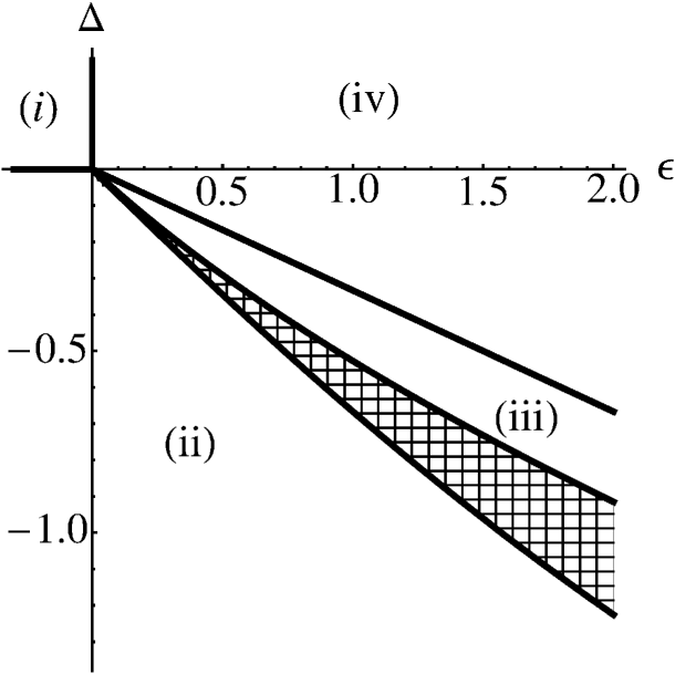
Figure 6: Regions of stability for the IR stable fixed points $({\it i})-({\it iv})$ in $(\epsilon,\Delta)$ plane.

For better illustration, regions of stability for fixed points $({\it i})-({\it iv})$ are depicted in Fig.6. Wee see that in contrast to the one-loop approximation Hnatic , overlap (dashed region) between regions of stability of fixed points $({\it ii})$ and $({\it iii})$ is observed. It is a common situation in the perturbative RG approach that higher order terms lead to either gap or overlap between neighbouring stability regions. The physical realization of the large-scale behavior then depends on the initial state of the system.

5 Long-time asymptotics of number density

Because the renormalization and calculation of the fixed points of the RG are carried out at two-loop level, we are able to find the first two terms of the $\epsilon$, $\Delta$ expansion of the average number density, which corresponds to solving the stationarity equations at the one-loop level. The simplest way to find the average number density is to calculate it from the stationarity condition of the functional Legendre transform Vasiliev (which is often called the effective action) of the generating functional obtained by replacing the unrenormalized action by the renormalized one in the weight functional. This is a convenient way to avoid any summing procedures used Lee94 to take into account the higher-order terms in the initial number density $n_{0}$.

5.1 Stationarity equations of the effective action

We are interested in the solution for the number density, therefore we put the expectation values of the fields ${\mathbf{v}}$ and $\tilde{{\mathbf{v}}}$ equal to zero at the outset (but retain, of course, the propagator and the correlation function). Therefore, at the second-order approximation the effective renormalized action for this model is

$$\Gamma_{R} = S_{1}+\frac{1}{4}\raisebox{-14.63881pt}{ \epsfbox{fig7.eps}}+\frac{1}{8}\raisebox{-14.63881pt}{ \epsfbox{fig8.eps}}+$$ (65)

$$\raisebox{-14.63881pt}{ \epsfbox{fig9.eps}}+\ldots\,,$$

where $S_{1}$ is the action (11) (within our convention $S_{2}=0$ in the effective action) and graphs are shown together with their symmetry coefficients. The slashed wavy line corresponds to the field $\psi^{\dagger}$ and the single wavy line to the field $\psi$. The stationarity equations for the variational functional

$$\frac{\delta\Gamma_{R}}{\delta\psi^{\dagger}}=\frac{\delta\Gamma_{R}}{\delta\psi}=0$$ (66)

give rise to the equations

$$\partial_{t}\psi=u\nu Z_{2}\nabla^{2}\psi-2\lambda u\nu\mu^{-2\Delta}Z_{4}\left(1+\psi^{\dagger}\right)\psi^{2}\\ +4u^{2}\nu^{2}\lambda^{2}\mu^{-4\Delta}\int\limits_{0}^{\infty}\!dt^{\prime}\int d{\mathbf{y}}\,(\Delta^{\psi\psi^{\dagger}})^{2}(t-t^{\prime},{\mathbf{x}}-{\mathbf{y}})\psi^{2}(t^{\prime},{\mathbf{y}})\\ +4u^{2}\nu^{2}\lambda^{2}\mu^{-4\Delta}\psi^{\dagger}(t,{\mathbf{x}})\\ \times\int\limits_{0}^{\infty}\!dt^{\prime}\int\!d{\mathbf{y}}\,(\Delta^{\psi\psi^{\dagger}})^{2}(t-t^{\prime},{\mathbf{x}}-{\mathbf{y}})\psi^{2}(t^{\prime},{\mathbf{y}})\\ +{\partial\over\partial x_{i}}\int\limits_{0}^{\infty}\!dt^{\prime}\int{\mathbf{y}}\,\Delta_{ij}^{vv}(t-t^{\prime},{\mathbf{x}}-{\mathbf{y}})\\ \times{\partial\over\partial x_{j}}\Delta^{\psi\psi^{\dagger}}(t-t^{\prime},{\mathbf{x}}-{\mathbf{y}})\psi(t^{\prime},{\mathbf{y}})+\ldots,$$ (67)

$$-\partial_{t}\psi^{\dagger}=u\nu Z_{2}\nabla^{2}\psi^{\dagger}-2\lambda u\nu\mu^{-2\Delta}Z_{4}\left[2\psi^{\dagger}+\left(\psi^{\dagger}\right)^{2}\right]\psi\\ +8u^{2}\nu^{2}\lambda^{2}\mu^{-4\Delta}\int\limits_{0}^{\infty}\!dt^{\prime}\int\!d{\mathbf{y}}(\Delta^{\psi\psi^{\dagger}})^{2}(t^{\prime}-t,{\mathbf{y}}-{\mathbf{x}})\psi^{\dagger}(t^{\prime},{\mathbf{y}})\times\\ \psi(t,{\mathbf{x}})+4u^{2}\nu^{2}\lambda^{2}\mu^{-4\Delta}\int\limits_{0}^{\infty}\!dt^{\prime}\int\!d{\mathbf{y}}(\Delta^{\psi\psi^{\dagger}})^{2}(t^{\prime}-t,{\mathbf{y}}-{\mathbf{x}})\\ \times\left[\psi^{\dagger}(t^{\prime},{\mathbf{y}})\right]^{2}\psi(t,{\mathbf{x}})\\ +\int\limits_{0}^{\infty}\!dt^{\prime}\int\!d{\mathbf{y}}\,\Delta_{ji}^{vv}(t^{\prime}-t,{\mathbf{y}}-{\mathbf{x}})\\ \times{\partial\over\partial x_{i}}\Delta^{\psi\psi^{\dagger}}(t^{\prime}-t,{\mathbf{y}}-{\mathbf{x}}){\partial\over\partial y_{j}}\psi^{\dagger}(t^{\prime},{\mathbf{y}})+\ldots$$ (68)

In (67) and (68), in the integral terms it is sufficient to put all renormalization constants equal to unity. Substituting the solution $\psi^{\dagger}=0$ of (68) into (67) we arrive at the fluctuation-amended rate equation in the form

$$\partial_{t}\psi=u\nu Z_{2}\nabla^{2}\psi-2\lambda u\nu\mu^{-2\Delta}Z_{4}\psi^{2}+\\ 4u^{2}\nu^{2}\mu^{-4\Delta}\lambda^{2}\int\limits_{0}^{\infty}\!dt^{\prime}\int\!d{\mathbf{y}}\,(\Delta^{\psi\psi^{\dagger}})^{2}(t-t^{\prime},{\mathbf{x}}-{\mathbf{y}})\psi^{2}(t^{\prime},{\mathbf{y}})\\ +{\partial\over\partial x_{i}}\int\limits_{0}^{\infty}\!dt^{\prime}\int\!d{\mathbf{y}}\,\Delta_{ij}^{vv}(t-t^{\prime},{\mathbf{x}}-{\mathbf{y}})\\ \times{\partial\over\partial x_{j}}\Delta^{\psi\psi^{\dagger}}(t-t^{\prime},{\mathbf{x}}-{\mathbf{y}})\psi(t^{\prime},{\mathbf{y}})+\ldots,$$ (69)

This is a nonlinear partial integro-differential equation, whose explicit solution is not known. It is readily seen that for a homogeneous solution the term resulting from the third graph in (65) vanishes and hence the influence of the velocity field on the homogeneous annihilation process would be only through the renormalization of the coefficients $\lambda$ and $D$. However, in case of a nonuniform density field $\psi$ the effect of velocity fluctuations is explicit in (69). Such a solution can be most probably found only numerically.

To arrive at an analytic solution, we restrict ourselves to the homogeneous number density $n(t)=\langle\psi(t)\rangle$, which can be identified with the expression (9). In this case the last term in (69) vanishes together with the Laplace operator term and the remaining coordinate integral may be calculated explicitly . The propagator is the diffusion kernel of the renormalized model (we consider first the system in the general space dimension $d$)

$$\Delta^{\psi\psi^{\dagger}}(t-t^{\prime},{\mathbf{x}})\\ =\frac{\theta(t-t^{\prime})}{\left[4\pi u\nu(t-t^{\prime})\right]^{d/2}}\exp\left[-\frac{x^{2}}{4u\nu(t-t^{\prime})}\right].$$ (70)

As noted above, for calculation of the one-loop contribution it is sufficient to put the renormalization constant $Z_{2}=1$ in the propagator $\Delta^{\psi\psi^{\dagger}}$. Therefore, evaluation of the Gaussian coordinate integral in (69) yields

$$\int\!d{\mathbf{y}}\,(\Delta^{\psi\psi^{\dagger}})^{2}(t-t^{\prime},{\mathbf{x}}-{\mathbf{y}})=\frac{\theta(t-t^{\prime})}{\left[8\pi u\nu(t-t^{\prime})\right]^{d/2}}$$ (71)

and we arrive at the ordinary integro-differential equation

$${{\rm d}n(t)\over{\rm d}t}=-2\lambda u\nu\mu^{-2\Delta}Z_{4}n^{2}(t)\\ +4\lambda^{2}u^{2}\nu^{2}\mu^{-4\Delta}\int\limits_{0}^{t}\!dt^{\prime}\,\frac{n^{2}(t^{\prime})}{\left[8\pi u\nu(t-t^{\prime})\right]^{d/2}}\,.$$ (72)

Spatial fluctuations in the number density show in the integral term and affect rather heavily even the homogeneous solution. In particular, the integral in (72) diverges at the upper limit in space dimensions $d\geq 2$. This is a consequence of the UV divergences in the model above the critical dimension $d_{c}=2$ and near the critical dimension is remedied by the UV renormalization of the model. To see this, subtract and add the term $n^{2}(t)$ in the integrand to obtain

$${{\rm d}n(t)\over{\rm d}t}=-2\lambda u\nu\mu^{-2\Delta}Z_{4}n^{2}(t)\\ +4\lambda^{2}u^{2}\nu^{2}\mu^{-4\Delta}n^{2}(t)\int\limits_{0}^{t}\!\frac{dt^{\prime}}{\left[8\pi u\nu(t-t^{\prime})\right]^{d/2}}\\ +4\lambda^{2}u^{2}\nu^{2}\mu^{-4\Delta}\int\limits_{0}^{t}\!dt^{\prime}\,\frac{n^{2}(t^{\prime})-n^{2}(t)}{\left[8\pi u\nu(t-t^{\prime})\right]^{d/2}}\,.$$ (73)

The last integral here is now convergent at least near two dimensions, provided the solution $n(t)$ is a continuous function. This is definitely the case for the iterative solution constructed below. The divergence in the first integral in (73) may be explicitly calculated below two dimensions and is canceled – in the leading order in the parameter $\Delta=(d-2)/2$ – by the one-loop term of the renormalization constant $Z_{4}$ (40). Expanding the right-hand side of (73) in the parameter $\Delta=(d-2)/2$ to the next-to-leading order we arrive at the equation

$${{\rm d}n(t)\over{\rm d}t}=-2\lambda u\nu\mu^{-2\Delta}n^{2}(t)\\ +2\lambda u\nu\mu^{-2\Delta}n^{2}(t)\left\{\frac{\lambda}{4\pi}\,\left[\gamma+\ln\left(2u\nu\mu^{2}t\right)\right]\right\}\\ +\frac{\lambda^{2}u\nu\mu^{-2\Delta}}{2\pi}\int\limits_{0}^{t}\!dt^{\prime}\,\frac{n^{2}(t^{\prime})-n^{2}(t)}{t-t^{\prime}}\,.$$ (74)

without divergences near two dimensions. Here, the factor $\mu^{-2\Delta}$ has been retained intact in order not to spoil the consistency of scaling dimensions in different terms of the equation. In (74), $\gamma=0.57721$ is Euler’s constant and we have considered the coupling constant $\lambda$ and the parameter $\Delta=(d-2)/2$ to be small parameters of the same order taking into account the magnitudes of the parameters in the basins of attraction of the fixed points of the RG.

The leading-order approximation for $n(t)$ is given by the first term on the right-hand side of (74) in the form

$$n^{(1)}(t)=\frac{n_{0}}{1+2{\lambda}u\nu t\mu^{-2\Delta}n_{0}}\,,$$ (75)

where $n_{0}$ is the initial number density. After substitution of this expression the integral term in (74) is of the order of $\lambda^{3}$ and thus negligible in the present next-to-leading-order calculation. Indeed, integration by parts in the integral in (74) yields

$$\int\limits_{0}^{t}\!dt^{\prime}\,\frac{n^{2}(t^{\prime})-n^{2}(t)}{t-t^{\prime}}=\lim_{\varepsilon\to 0}\int\limits_{0}^{t-\varepsilon}\!dt^{\prime}\,\frac{n^{2}(t^{\prime})-n^{2}(t)}{t-t^{\prime}}\\ =\left[n_{0}^{2}-n^{2}(t)\right]\ln t+2\int\limits_{0}^{t}\!dt^{\prime}\,\ln(t-t^{\prime})n(t^{\prime}){{\rm d}n(t^{\prime})\over{\rm d}t^{\prime}}\,.$$ (76)

From (74) it is readily seen that $\displaystyle{{\rm d}n(t)\over{\rm d}t}=O\left(\lambda\right)$. From the explicit expression (75) it follows that $n^{2}(t)-n_{0}^{2}=O\left(\lambda\right)$ as well. Therefore, in the iterative solution of (74) the term with the integral on the right side is of the order of $\lambda^{3}$.

In this approximation, Eq. (74) yields

$$n(t)=\\ \frac{n_{0}}{1+2{\lambda}u\nu t\left\{1+\frac{\displaystyle\lambda}{\displaystyle 4\pi}\left[1-\gamma-\ln\left(2u\nu\mu^{2}t\right)\right]\right\}\mu^{-2\Delta}n_{0}}\,,$$ (77)

where $n_{0}$ is the initial number density.

5.2 Asymptotic behavior of the number density

We shall use the next-to-leading order iterative solution (77) of the stationarity equation (74) as the initial condition of the RG equation for the number density to evaluate the long-time asymptotic behavior of the number density. The RG equation is obtained by applying the RG differential operator (45) to the renormalized number density $n(t)$.

Since the fields $\Phi=\{v,\tilde{v},\psi,\psi^{\dagger}\}$ are not renormalized, the renormalized connected Green functions $W$ differ from the unrenormalized $W_{0}=\langle\Phi\ldots\Phi\rangle$ Vasiliev04 only by the choice of parameters and thus one may write

$$W(g,\nu,\mu,\ldots)=W_{0}(g_{0},\nu_{0},\ldots),$$ (78)

where $g_{0}=\{g_{10},g_{20},u_{0},\lambda_{0}\}$ is the full set of the bare parameters and dots denotes all variables unaffected by the renormalization procedure. The independence of the renormalized number density $n(t)$ of the renormalization mass parameter $\mu$ is expressed by the equation

$$D_{RG}n(t,\mu,\nu,n_{0},g)=0\,.$$

Using this equation together with the explicit expression for the RG differential operator (45) the RG equation for the mean number density $n(t)$ is readily obtained:

$$\left(\mu\frac{\partial}{\partial\mu}+\sum\limits_{g_{i}}\beta_{g_{i}}\frac{\partial}{\partial g_{i}}-\gamma_{1}\nu\frac{\partial}{\partial\nu}\right)n(t,\mu,\nu,n_{0},g)=0.$$ (79)

We are interested in long-time behavior of the system ($t\rightarrow\infty$), therefore we trade the renormalization mass for the time variable. According to the canonical dimensions of parameters and fields in Table 1, the Euler equations with respect to the wave number and time assume the form Adzhemyan99

$$\left(\mu\frac{\partial}{\partial\mu}-2\nu\frac{\partial}{\partial\nu}+dn_{0}\frac{\partial}{\partial n_{0}}-d\right)n(t,\mu,\nu,n_{0},g)=0,$$ (80)

$$\left(-t\frac{\partial}{\partial t}+\nu\frac{\partial}{\partial\nu}\right)n(t,\mu,\nu,n_{0},g)=0,$$ (81)

where the first equation expresses scale invariance with respect to wave number and the second equation with respect to time. Eliminating partial derivatives with respect to the renormalization mass $\mu$ and viscosity $\nu$ from (79), (80) and (81) we obtain the Callan-Symanzik equation for the mean number density:

$$\biggl{[}(2-\gamma_{1})t\frac{\partial}{\partial t}+\sum_{g}\beta_{g}\frac{\partial}{\partial g}-dn_{0}\frac{\partial}{\partial n_{0}}+d\biggr{]}n\left(t,\mu,\nu,n_{0},g\right)=0$$ (82)

To separate information given by the RG, consider the dimensionless normalized mean number density

$$\frac{n}{n_{0}}=\phi\left(\nu\mu^{2}t,\lambda u\,\frac{n_{0}}{\mu^{d}},g\right)\,.$$ (83)

For the asymptotic analysis, it is convenient to express the initial number density $n_{0}$ as an argument of the function $\phi$ in the combination used here.

Solution of (82) by the method of characteristics yields

$$\phi\left(\nu\mu^{2}t,\lambda u\,{n_{0}\over\mu^{d}},g\right)=\phi\left({\nu}\mu^{2}\tau,\overline{\lambda}\overline{u}\,{\overline{n}_{0}\over\mu^{d}},\overline{g}\right)$$ (84)

where $\tau$ is the time scale. In Eq. (84), $\overline{g}$ and $\overline{n}_{0}$ are the first integrals of the system of differential equations

$$t\frac{d}{dt}\overline{g}=-\frac{\beta_{g}(\overline{g})}{2-\gamma_{1}(\overline{g})}\,,\quad t\frac{d}{dt}\overline{n}_{0}=d\frac{\overline{n}_{0}}{2-\gamma_{1}(\overline{g})}.$$ (85)

Here $\overline{g}=\{\overline{g_{1}},\overline{g_{2}},\overline{u},\overline{\lambda}\}$ with initial conditions $\overline{g}|_{t=\tau}=g$ and $\overline{n}_{0}|_{t=\tau}=n_{0}$. In particular,

$$\overline{\lambda}\overline{u}\overline{n}_{0}=\lambda u\,n_{0}\,\left({t\over\tau}\right)\exp\left[{\displaystyle\int_{\tau}^{t}{\displaystyle\gamma_{4}ds\over\displaystyle(2-\gamma_{1})s}}\right]\,.$$ (86)

From here it follows that the asymptotic expression of the integral on the right-hand side of (86) in the vicinity of the IR-stable fixed point $g^{*}$ is of the form

$${\int_{\tau}^{t}{\displaystyle\gamma_{4}ds\over\displaystyle(2-\gamma_{1})s}}\operatornamewithlimits{\sim}_{t\to\infty}{\gamma_{4}^{*}\over 2-\gamma_{1}^{*}}\ln\left({t\over\tau}\right)\\ +{2\over 2-\gamma_{1}^{*}}\int\limits_{\tau}^{\infty}\!{(\gamma_{4}-\gamma_{4}^{*})ds\over(2-\gamma_{1})s}={\gamma_{4}^{*}\over 2-\gamma_{1}^{*}}\,\ln\left({t\over\tau}\right)+\tilde{c}_{4}(\tau)\,,$$ (87)

corrections to which vanish in the limit $t\to\infty$. In (87) and henceforth, the notation $\gamma_{1}^{*}=\gamma_{1}\left(g^{*}\right)$ has been used.

From the point of view of the long-time asymptotic behavior the next-to-leading term in (87) is an inessential constant. From (86) and (87) it follows that in the vicinity of the fixed point

$$\overline{\lambda}\overline{u}\,{\overline{n}_{0}\over\mu^{d}}\sim\lambda u\,{n_{0}\over\mu^{d}}\left({t\over\tau}\right)^{\displaystyle 1+{\displaystyle\gamma_{4}^{*}\over\displaystyle 2-\gamma_{1}^{*}}}\widetilde{C}_{n}\\ \equiv\lambda u\,{n_{0}\over\mu^{d}}\left({t\over\tau}\right)^{\alpha}\widetilde{C}_{n}\equiv\overline{y}\,\widetilde{C}_{n}\,,$$ (88)

where a shorthand notation $\overline{y}$ has been introduced for the long-time scaling of the normalized number density as well as the dimensional normalization constant

$$\widetilde{C}_{n}=e^{d\tilde{c}_{4}(\tau)}\,.$$

and the decay exponent

$$\alpha=\displaystyle 1+{\displaystyle\gamma_{4}^{*}\over\displaystyle 2-\gamma_{1}^{*}}$$ (89)

The asymptotic behavior of the normalized number density is described by the scaling function $f(x,y)$:

$$\phi\left(\nu\mu^{2}t,\lambda u\,{n_{0}\over\mu^{d}},g\right)\\ \sim\phi\left({\nu}\mu^{2}\tau,\widetilde{C}_{n}\overline{y},{g}^{*}\right)\equiv f\left({\nu}\mu^{2}\tau,\widetilde{C}_{n}\overline{y}\right)\,.$$ (90)

The scaling function $f(x,y)$ describing the asymptotic behavior of the normalized number density $\phi=n/n_{0}$ is a function of two dimensionless argument only, whereas the generic $\phi$ has six dimensionless arguments (all four coupling constants on top of the scaling arguments of $f(x,y)$). We recall that the generic solution of the Callan-Symanzik equation (82) does not give the explicit functional form of the function $n=n_{0}\phi$, which may to determined from the solution (77) of the stationarity equation of the variational problem for the effective potential. The free parameters left in the variables of the scaling function $f(x,y)$ correspond to the choice of units of these variables, whereas the objective information is contained in the form of the scaling function Vasiliev04 ; Adzhemyan99 .

From the explicit solution (77) we obtain the generic expression

$$h(x,y)={1\over f(x,y)}\\ =1+2xy\left\{1+{\displaystyle{{\lambda}^{*}}\over\displaystyle 4\pi}\left[1-\gamma-\ln\left(2u^{*}x\right)\right]\right\}\,,$$ (91)

the substitution in which of the various fixed-point values $\lambda^{*}$ (at the leading order $\lambda^{*}\approx 2\pi\overline{\lambda}^{*}$) and $u^{*}$ in the leading approximation together with the substitution of $x=\nu\mu^{2}\tau$ and $y=\tilde{C}\overline{y}$ from (88) and (89) yields the corresponding $\varepsilon$, $\Delta$ expansions of the asymptotic expression of the normalized number density.

Below, we list the scaling functions $h(x,y)$ and the dynamic exponents $\alpha$ at the stable fixed points in the next-to-leading-order approximation.
(i ) At the trivial (Gaussian) fixed point (53) the mean-field behavior takes place with

$$h(x,y) =1+2xy\,,$$

$$\alpha =1\,.$$ (92)

(ii ) The thermal (short-range) fixed point (4) leads to scaling function and decay exponent

$$h(x,y) =1+2xy\left\{1-{\displaystyle{\Delta}\over\displaystyle 2}\left[1-\gamma-\ln\left(\sqrt{17}-1\right)\,x\right]\right\}\,,$$

$$\alpha =1+{\Delta\over 2}+{\Delta^{2}\over 2}\,.$$ (93)

Here, the last coefficient is actually a result of numerical calculation, which in the standard accuracy of Mathematica is equal to 0.5. We have not been able to sort out this result analytically, but think that most probably the coefficient of the $\Delta^{2}$ term in the decay exponent $\alpha$ in (5.2) really is ${1\over 2}$.
(iii ) The kinetic fixed point with an anomalous reaction rate (58) corresponds to

$$h(x,y) = 1+2xy\biggl{\{}1-{\displaystyle{\epsilon+3\Delta}\over\displaystyle 3}\times$$

$$\left[1-\gamma-\ln\left(\sqrt{17}-1\right)\,x\right]\biggl{\}}\,,$$

$$\alpha = 1+{3\Delta+\epsilon\over 3-\epsilon}\,,$$ (94)

with an exact value of the decay exponent.
(iv ) At the kinetic fixed point with mean-field-like reaction rate (61) we obtain

$$h(x,y) =1+2xy\,,$$

$$\alpha =1\,.$$ (95)

In the actual asymptotic expression corresponding to (90) the argument $y\to\widetilde{C}_{n}\overline{y}$ is different from that of the Gaussian fixed point.

5.3 Asymptotic behavior in two dimensions

To complete the picture, we recapitulate – with a little bit more detail – the asymptotic behavior of the number density in the physical space dimension $d=2$ predicted within the present approach Hnatic (it turns out that for these conclusions the one-loop calculation is sufficient). On the ray $\varepsilon\leq 0$, $\Delta=0$ logarithmic corrections to the mean-field decay take place. The integral determining the asymptotic behavior of the variable (86) yields in this case

$${\int_{\tau}^{t}{\displaystyle\gamma_{4}ds\over\displaystyle(2-\gamma_{1})s}}\operatornamewithlimits{\sim}_{t\to\infty}-{1\over 2}\,\ln\ln\left({t\over\tau}\right)+\tilde{c}_{4}(\tau)\,,$$ (96)

with corrections vanishing in the limit $t\to\infty$. Therefore, in the vicinity of the fixed point

$$\overline{\lambda}\overline{u}\,{\overline{n}_{0}\over\mu^{d}}\sim\lambda u\,{n_{0}\over\mu^{d}}\left({t\over\tau}\right)\ln^{-1/2}\left({t\over\tau}\right)\widetilde{C}_{n}\equiv\overline{y}\,\widetilde{C}_{n}\,.$$ (97)

The scaling function $h$ is of the simple form

$$h(x,y)=1+2xy$$

and gives rise to asymptotic decay slower than in the mean-field case by a logarithmic factor:

$${n}\sim{\ln^{1/2}\left(t/\tau\right)\over 2\nu\lambda u\widetilde{C}_{n}t}\,.$$

It is worth noting that this logarithmic slowing down is weaker than that brought about the density fluctuations only Peliti and this change is produced even by the ubiquitous thermal fluctuations of the fluid, when the reaction is taking place in gaseous or liquid media.

On the open ray $\varepsilon>0$, $\Delta=0$ the kinetic fixed point with mean-field-like reaction rate (61) is stable and the asymptotic behavior is given by (5.2) regardless of the value of the falloff exponent of the random forcing in the Navier-Stokes equation. In particular, only the amplitude factor in the asymptotic decay rate in two dimensions is affected by the developed turbulent flow with Kolmogorov scaling, which corresponds to the value $\varepsilon=2$. This is in accord with the results obtained in the case of quenched solenoidal flow with long-range correlations Deem2 ; Tran as well as with the usual picture of having the maximal reaction rate in a well-mixed system.

6 Conclusion

In conclusion, we have analyzed the effect of density and velocity fluctuations on the reaction kinetics of the single-species decay $A+A\to\emptyset$ universality class in the framework of field-theoretic renormalization group and calculated the scaling function and the decay exponent of the mean number density for the four asymptotic patterns predicted by the RG.

We have calculated the relevant renormalization constants at two-loop level and found the decay exponent of the mean number density at this order of the $\epsilon$, $\Delta$ expansion for four IR stable fixed points of the RG, whose regions of stability cover the whole parametric space in the vicinity of the origin in the $\epsilon$, $\Delta$ plane. The decay exponent assumes the mean-field value in the basins of attraction of the trivial fixed point (53) and of the kinetic fixed point (61) with dominant fluctuations of the random force of the Navier-Stokes equation. At the kinetic fixed point with finite rate coefficient (58) the value of the decay exponent is determined exactly by the fixed-point equations. At the thermal (short-range) fixed point (4) the decay exponent possesses a non-trivial $\epsilon$, $\Delta$ expansion. We have calculated three first terms of this expansion and thus pushed its accuracy by one order further than in in the one-loop calculation as well as in the case of kinetic fixed point with anomalous reaction rate. We have also found an overlap between the regions of stability of these two asymptotic patterns, which means that the asymptotic behavior of system depends on the details of the approach to the fixed point.

Using a variational approach, we have inferred a renormalized fluctuation-amended rate equation with the account of one-loop corrections, which again is a step forward in the accuracy of description of the system and opens the possibility to analyze direct effects of on the number density of the velocity fluctuations, which do not enter explicitly in the leading-order mean-field rate equation. This non-linear integro - differential equation has been solved iteratively in the framework of the $\epsilon$, $\Delta$ expansion and the scaling function for the mean number density has been calculated for the four IR stable regimes. The scaling function assumes the mean-field form (exactly) in the basins of attraction of the trivial fixed point and the kinetic fixed point with dominant fluctuations of the random force. At the kinetic fixed point with finite rate coefficient and at the thermal fixed point the scaling function possesses a non-trivial $\epsilon$, $\Delta$ expansion, which we have calculated at the linear order.

Fluctuations of the random advection field affect heavily the long-time asymptotic behavior of the system: the kinetic fixed points are brought about by the velocity fluctuations as well as the non-trivial series expansion of the decay exponent at the thermal fixed point (without velocity fluctuations, the decay exponent is fixed to the one-loop value, because there are no high-order corrections to the rate constant in this case). Predictions of the renormalization-group analysis for the reaction $A+A\to\emptyset$ in quenched random fields have been corroborated by numerical simulations Chung ; Tran . In the case of dynamically generated random drift this is seems to be a much more demanding task, but would surely be highly desirable, since the experimental data for reaction processes is quite scarce Tauber05 .

The integro-differential equation for the calculation of the concentration proposed here and solved analytically in a suitable approximation allows for heterogeneous solutions as well. Since the heterogeneous concentration most probably has to be found numerically, analysis of this issue is beyond the scope of the present paper. We intend to carry out this investigation in the near future, all the more so because there is significant recent interest in the effect of random drift on nonlinear diffusion equations Tel05 ; Benzi12 , to which the stationarity equations of the proposed variational functional belong. However, most of these problems include competition between growth and decline of population and give rise to more complicated models than that at hand. The potential of the field-theoretic approach in analytic investigation of stochastic problems is, however, far from being exhausted, therefore in the future we hope to deal with the diffusion-limited birth-death processes in random flows within this framework as well.

Appendix A Explicit form of the renormalization constants

The coefficient functions $A_{ij}$ and $B_{ij}$ of the renormalization constant (39) are

$$A_{11} =-\frac{(1+\xi)u^{2}+(3\xi+2)u+6\xi+1}{512u(1+u)^{3}\xi},$$

$$A_{12} =-\frac{(1+\xi)u^{2}+(1+3\xi)u+6\xi-4}{256u(1+u)^{3}(1-\xi)},$$

$$A_{22} =-\frac{u+5}{512u(1+u)^{3}},$$

$$B_{11} =B_{1}(u)+B_{2}(u,\xi),$$

$$B_{12} =4[B_{1}(u)+B_{3}(u,\xi)],$$

$$B_{22} =-B_{1}(u)-B_{2}(u,-1),$$

where the functions $B_{1},B_{2}$ and $B_{3}$ are given as

$$\begin{split}&B_{1}(u)=\frac{1}{1024u^{4}(1+u)^{3}(u-1)}\biggl{[}\\ &-12u^{3}(1+u)\ln\frac{2}{1+u}+32u^{4}(1+u)^{2}\ln 2\\ &+2u^{3}(1+u)^{2}(u+10)\ln\frac{4}{3}-32u^{3}(1+u)^{3}{\rm artanh}\frac{1}{2}\\ &+4(2u^{6}+6u^{5}+7u^{4}+10u^{3}-4u-1)\ln\frac{1+2u}{(1+u)^{2}}\\ &-4u^{3}(1+u)[4u^{2}+20u+9]\ln\frac{1+2u}{2+2u}\\ &+16u^{3}(1+u)^{3}{\rm artanh}\frac{u}{u+1}\\ &+8u^{3}(1+u)^{2}(u-1)(\gamma+\psi(3/2))\\ &-u^{2}(23u^{4}+38u^{3}+17u^{2}+22u+4)\biggl{]}\\ &-\frac{1}{128\pi u(1+u)^{2}(u-1)}\int_{1}^{\infty}dq\int_{-1}^{1}dzF(q,z,u)\,,\end{split}$$

$$B_{2}(u,\xi)=\xi\frac{(2+4\xi)u^{2}+(10\xi+8)u+38+22\xi}{1024u(1+u)^{3}(2+\xi)},$$

$$B_{3}(u,\xi)=-\frac{(8\xi+4)u^{2}+(14\xi+10)u+22-10\xi}{1024u(1+u)^{3}}$$

with the function $F$ given by the expression

$$F(x,z,u)=(1-z^{2})^{1/2}\frac{M(x,z,u)}{N(x,z,u)}$$

$$\begin{split}&M(x,z,u)=(x^{6}+1)[z^{3}(24u^{3}+24u^{2}+72u+72)\\ &-z(8u^{3}+12u^{2}+8u+60)]+(x^{5}+x)[-z^{4}(40u^{3}\\ &+88u^{2}+120u+264)+z^{2}(-4u^{3}+16u^{2}+108u+168)\\ &+4u^{3}+14u^{2}+28u+18]+(x^{4}+x^{2})[z^{5}(16u^{3}+96u^{2}\\ &+48u+288)+z^{3}(12u^{4}+64u^{2}+128u^{2}+96u+180)\\ &-z(4u^{4}+26u^{3}+92u^{2}+174u+312)]+x^{3}[-z^{6}(32u^{2}\\ &+96)-z^{4}(8u^{4}+64u^{3}+240u^{2}+144u+600)\\ &+z^{2}(-8u^{4}+4u^{3}+84u^{2}+108u+452)+2u^{4}+6u^{3}\\ &+26u^{2}+58u+36],\end{split}$$

$$N(x,z,u)=(1+x^{2}-2xz)(1+x^{2}-xz)$$

$$\times((1+u)x^{2}+2-2xz)(1+u+2x^{2}-2xz)\,.$$

The coefficient function $C$ of the renormalization constant (40) is

$$\begin{split}C(u,\xi)&=-\frac{1}{8u\pi}\int_{-1}^{1}dz(1-z^{2})^{\frac{1}{2}}G(z,u)\\ &+\frac{1}{8u(1+u)}\biggl{(}\ln\frac{1+u}{2u}+1+\frac{2+u}{u}\ln\frac{u+2}{2u+2}+\xi\biggl{)},\end{split}$$

where

$$\begin{split}&G(z,u)=\frac{4}{(1-u)^{2}+4uz^{2}}\biggl{\{}\frac{u-1}{2}\ln\frac{2u}{1+u}\\ &-\frac{2(1+u)z}{\sqrt{1-z^{2}}}\biggl{[}\frac{\pi}{2}-\arctan\sqrt{\frac{1+z}{1-z}}\biggl{]}\\ &+\frac{u(u+3)z}{\sqrt{2u(1+u)-u^{2}z^{2}}}\biggl{[}\pi-\arctan\frac{zu+u+1}{\sqrt{2u(1+u)-u^{2}z^{2}}}\\ &-\arctan\frac{(2+z)u}{\sqrt{2u(1+u)-u^{2}z^{2}}}\biggl{]}\biggl{\}}\,.\end{split}$$

Appendix B Fixed points

The coefficient functions of the fixed points (58) and (61) are

$$\begin{split}&u_{1}^{*}(\xi)=\frac{8R}{3\sqrt{17}}-\frac{8192}{3\sqrt{17}}B_{1}(u^{*}_{0})-\frac{1}{432\sqrt{17}(1+\xi)^{2}(2+\xi)}\\ &\times\biggl{[}(21384-648\sqrt{17})\xi^{4}\\ &+(52512-2592\sqrt{17})\xi^{3}+(22192-2736\sqrt{17})\xi^{2}\\ &+(72\sqrt{17}-29064)\xi+720\sqrt{17}-18768\biggl{]}\,,\end{split}$$

$$\begin{split}&g_{12}^{*}(\xi)=64\frac{R(2+3\xi)-1}{27(1+\xi)}\\ &-16\frac{2+3\xi}{243(1+\xi)^{4}(2+\xi)}\biggl{[}45\xi^{4}+213\xi^{3}+349\xi^{2}+231\xi+50\biggl{]}\,,\end{split}$$

$$\begin{split}&g_{22}^{*}(\xi)=64\frac{1+R}{27(1+\xi)}\\ &-16\frac{2+3\xi}{243(1+\xi)^{4}(2+\xi)}\biggl{[}57\xi^{4}+171\xi^{3}+185\xi^{2}+93\xi+22\biggl{]}\,.\end{split}$$

References

- (1) B. Derrida, V. Hakim and V. Pasquier, Phys. Rev. Lett. 75, (1995) 751.
- (2) R. Kroon, H. Fleurent and R. Sprik, Phys. Rev. E 47, (1993) 2462
- (3) N. G. van Kampen, Stochastic processes in Physics and Chemistry (North-Holland, Amsterdam 1984)
- (4) K. Kang and S. Redner, Phys. Rev. A 32, (1985) 435.
- (5) B. P. Lee, J. Phys. A 27, (1994) 2633.
- (6) J. L. Cardy and U. C. Tauber, Phys. Rev. Lett. 77, (1996) 4780.
- (7) C. Itzykson and J.-M. Drouffe, Statistical Field Theory: Volume 1 (Cambridge University Press, 1991)
- (8) J.-M. Park and M. W. Deem, Phys. Rev. E 57, (1998) 3618.
- (9) W.J. Chung and M. W. Deem, Physica A 265, (1999) 486.
- (10) M. J. E. Richardson and J. Cardy, J. Phys. A 32, (1999) 4035.
- (11) M. W. Deem and J.-M. Park, Phys. Rev. E 58, (1998) 3223.
- (12) N. le Tran,J.-M. Park and M. W. Deem, J. Phys. A 32, (1999) 1407.
- (13) M. Hnatich and J. Honkonen, Phys. Rev. E 61, (2000) 3904.
- (14) U. Frisch, Turbulence: The Legacy of A. N. Kolmogorov (Cambridge University Press, 1995)
- (15) D. Forster, D. R. Nelson and M. J. Stephen, Phys. Rev. Lett. 36, (1976) 867.
- (16) D. Forster, D. R. Nelson and M. J. Stephen, Phys. Rev. A 16, (1977) 732.
- (17) L. Ts. Adzhemyan, A. N. Vasil’ev and Yu. M. Pis’mak, Teor. Mat. Fiz. 57, (1983) 268.
- (18) M. Doi, J. Phys. A 9, (1976) 1465.
- (19) M. Doi, J. Phys. A 9, (1976) 1479.
- (20) L. Peliti, J. Phys. A 19, (1986) L365.
- (21) A. N. Vasil’ev, Functional Methods in Quantum Field Theory and Statistical Physics (Gordon and Breach, Amsterdam, 1998)
- (22) C. De Dominicis and P. C. Martin, Phys. Rev. A 19, (1979) 419.
- (23) A. N. Vasil’ev, The Field Theoretic Renormalization Group in Critical Behavior Theory and Stochastic Dynamics (Boca Raton: Chapman Hall/CRC, 2004)
-
(24)
H. K. Janssen, Z. Phys. B 23, 377 (1976) ;
R. Bausch, H. K. Janssen a H. Wagner, Z. Phys. B 24, 113 (1976). - (25) J. Zinn-Justin, Quantum Field Theory and Critical Phenomena (Oxford Univ. Press, Oxford, 1989)
- (26) L. Ts. Adzhemyan, J. Honkonen, M. V. Kompaniets and A. N. Vasil’ev, Phys. Rev. E 71, (2005) 036305.
- (27) L. Ts. Adzhemyan, N. V. Antonov and A. N. Vasiliev, The Field Theoretic Renormalization Group in Fully Developed Turbulence (Gordon and Breach, Amsterdam, 1999)
- (28) L.Ts. Adzhemyan, N. V. Antonov and J. Honkonen, Phys. Rev. E 66, (2002) 036313.
- (29) M. Hnatich, J. Honkonen, Horvath and R. Semancik, Phys. Rev. E 59, (1999) 4112.
- (30) U. C. Täuber, M. Howard and B. P. Vollmayr-Lee, J. Phys. A: Math. Gen. 38, (2005) R79.
- (31) T. Tél, A. de Moura, C. Grebogi and G. Károlyi, Phys. Rep. 413, (2005) 91.
- (32) R. Benzi, M. H.Jensen, D. R.Nelson, P. Perlekar, S. Pigolotti, and F. Toschi, Population dynamics in compressible flows, (2012) 1203.6319v1 [q-bio.PE].