A two-speed model for finite-strain elasto-plasticity

Abstract.

This work presents a new modeling approach to macroscopic, polycrystalline elasto-plasticity starting from first principles and a few well-defined structural assumptions, incorporating the mildly rate-dependent (viscous) nature of plastic flow and the microscopic origins of plastic deformations. For the global dynamics, we start from a two-stage time-stepping scheme, expressing the fact that in most real materials plastic flow is much slower than elastic deformations, and then perform a detailed analysis of the slow-loading limit passage. In this limit, a rate-independent evolution can be expected, but this brings with it the possibility of jumps (relative to the “slow” time). Traditionally, the dynamics on the jump transients often remain unspecified, which leads to ambiguity and deficiencies in the energy balance. In order to remedy this, the present approach precisely describes the energetics on the jump transients as the limit of the rate-dependent evolutions at “singular points”. It turns out that rate-dependent behavior may (but does not have to) prevail on the jump transients. Based on this, we introduce the new solution concept of “two-speed solutions” to the elasto-plastic evolutionary system, which incorporates a “slow” and a “fast” time scale, the latter of which parametrizes the jump transients.

MSC (2010): 74C15 (primary); 74C20, 35Q74, 74H10 (secondary).

Keywords: Elasto-plasticity, slow-loading limit, rate-independent system, quasi-static evolution, two-speed solution.

Date: (version 1.0).

1. Introduction

The theoretical modelling of large-strain elasto-plasticity for polycrystalline materials poses many challenges and, despite its great importance, no fully satisfactory mathematical theory has emerged so far. Works in this direction include for instance [17, 50, 35, 47, 9, 31, 46, 57, 48, 37, 14] as well as the monographs [30, 32, 19, 21]. Some major issues in the quest for such a theory are the following: First, elasto-plasticity naturally goes beyond what can be modeled in a traditional continuum mechanics framework. Rather, a body undergoing plastic flow does not remain a continuum as the material is internally “ripped and torn”, even if this is not macroscopically observable. Even if one is not interested in precisely describing the microscopic origins of plastic flow (such as dislocation movement in metals, see for instance [26, 8, 23, 1, 53, 22]), some aspects of the microscopic situation need to be taken into account in order to derive a consistent theory. More advanced mathematical structures such as Lie groups and Lie algebras, can be very effective in describing the relationships between macroscopic and microscopic phenomena, but are rarely used in the engineering literature (but see [37]).

Second, when deriving the full dynamics of the material, it is often unclear how the solid-like elastic deformations and the fluid-like plastic deformations interact. In particular, their relative speed plays an important role, but this does not seem to be used at present for plasticity modelling.

Third, elasto-plastic flow is rate-dependent (viscous) in reality, but only slightly so, and thus rate-independent (quasi-static) approximations are used more often than not. However, this simplification creates the serious problem that the regularity of solution processes can only be low in general since jumps (relative to the “slow” time scale) can occur in rate-independent processes – at least there is no obvious mechanism preventing this a-priori. This creates the need to specify the behavior of the evolution on the jump transients, which is important for the global energetics, but rarely considered.

The present work develops, from first principles, a model of macroscopic elasto-plasticity that aims to addresses the above issues, and then to analyze it. Our approach is based on the following key principles:

1. Macroscopic deformations are modeled as driven by microscopic slips (e.g. slips induced by dislocation movement), an idea taken from single-crystal plasticity. This idea can be abstractly expressed using the theory of Lie groups and their Lie algebras: A matrix from a Lie group represents the macroscopic plastic distortion and hence (part of) the internal state of the material. The plastic flow, however, is specified on the level of the associated “microscopic” Lie algebra (i.e. the tangent space at the identity matrix) as the sum of microscopic drifts (slip rates) acting as infinitesimal generators of the flow. The main advantage of the Lie-theoretic point of view expressed in this work is that on the microscopic Lie algebra level we are dealing with a linear structure.

2. Elastic movements are assumed to be infinitely fast relative to the plastic ones, which is quite realistic [3, 4], so we base the model on the postulate that the system minimizes over all admissible elastic, but not plastic, deformations.

3. The plastic dynamics are first modeled as rate-dependent, i.e. viscous. If the system is spontaneously pushed out of a stable (rest) state, it relaxes to stability by following an evolutionary flow rule. Unlike other models (see below for comparisons), here we do not rely on minimization over irreversible movements, which is thermodynamically questionable. In particular, we work with the realistic local stability (yield) condition in the slow-loading limit.

4. The combined elasto-plastic dynamics are modeled based on a two-stage time-stepping scheme, which alternates between two “fundamental motions”: purely elastic minimization and elasto-plastic relaxation, the latter exchanging elastic for plastic distortion without modifying the total deformation. This two-stage approach allows for a very clean modeling without any ambiguity as to which test functions should be considered in the principle of virtual power.

5. Via a slow-loading limit passage we arrive at the limit “two-speed” formulation, which incorporates two time scales: With respect to the “slow” time, the formulation is rate-independent. On jump transients, however, we retain the possibility of rate-dependent evolution (or a mixture of rate-dependent and rate-independent evolution) with respect to the “fast” time.

6. We formulate the whole model in the reference frame, but point out how the common formulation with structural (intermediate) tensors is essentially equivalent via Lie group adjoints. We do not use the idea of an “intermediate (structural) space” since one cannot consistently define “intermediate points”.

If $y\colon\Omega\subset\mathbb{R}^{3}\to\mathbb{R}^{3}$ denotes the total deformation of our specimen, then the commonly used Kröner–Lee decomposition

$$\nabla y=F=EP$$

splits the deformation gradient into elastic and plastic distortions $E,P$; since $E,P$ are not in general curl-free, they might not be deformation gradients themselves. We refer to  [25, 28, 27, 17, 5, 19, 49] for justifications and various other aspects of this decomposition. Note in particular that if $\operatorname{curl}P\neq 0$, then $E$ cannot be the identity map; this expresses the physical constraint that the elastic deformation has to close the gaps opened by the plastic flow so as to restore a macroscopic continuum.

The multiplicative Kröner–Lee decomposition is at the root of many mathematical challenges in large-strain theories of elasto-plasticity. Not only is it incompatible with our traditional linear function spaces, the splitting of $\nabla y$ into $E$ and $P$ furthermore is clearly not unique. The ensuing ambiguity (often called the “uniqueness problem” in the literature) is a big obstacle when trying to develop a useful mathematical theory. For instance, if for the moment we consider the macroscopic elasto-plastic flow to be divided into a number of time intervals $[t_{k},t_{k+1})$, $k=0,\ldots,N-1$, then in every such interval we have potentially both an elastic and a plastic distortion, $E_{k},P_{k}$ say. Macroscopically, the total plastic distortion should be $P=P_{N}P_{N-1}\cdots P_{0}$. However, if we let $N\to\infty$ (the interval size going to zero), even this “natural” setup seems to lead to the need for infinite products, which is not feasible due to the non-commutativity of matrix multiplication. For example, an approach using matrix logarithms to transform products into sums runs into trouble since the involved matrices are not necessarily symmetric and positive definite, whereby the matrix logarithm might not be uniquely definable. We here posit that the plastic distortion $P$ can only be determined from the internal state of the material and its flow in time needs to be specified through a differential equation, see [19] some discussion on this point. This approach removes all ambiguity in the Kröner–Lee decomposition.

Another feature of the present model, reminiscent of recent work by Reina & Conti [49], is that we study the structure of microscopic slips via a reasoning with functions of bounded variation (see [13, 2]) whose derivative contains an absolute continuous (elastic) part and a singular (plastic) part. On the microscopic level these two parts must decompose additively since they take place in different parts of the material (bulk and surface parts, respectively). In the macroscopic “homogenized” theory, however, this separation is lost and we keep track of the plastic distortion rate (speed) via an equation in the “microscopic” Lie group.

Previous mathematical theories for large-strain elasto-plasticity seem to fall into one of two categories: The first, energetic, approach was introduced in [48, 43, 45, 44] and applied to nonlinear elasto-plasticity in [37, 33, 14, 38, 34]. It starts from a time discretization and assumes that the system at every time step minimizes the potential energy plus any dissipational cost that may be incurred by jumping to the target state. In the limit, a global form of the stability (yield) condition and an energy balance can be derived (these two conditions alone, however, can have more solutions than the original time-discrete scheme, see [39]). The global, dissipative minimization in the time-stepping scheme assumes infinite foresight of the system since one may jump to an (energetically) far-away state, even if there is a potential energy barrier in the way, so the system can in fact jump “too early” and “too far”. Moreover, from a physical perspective, minimization over irreversible (dissipative) movements seems to be a violation of the Second Law of Thermodynamics. Nevertheless, if these assumptions are a good approximation to the physical situation at hand, then a very mature theory is available; the current state-of-the-art is presented in the recent monograph [42], also see [55, 56] for a global variational principles in this context.

A more recent approach to address the under-specification of the system’s behavior on jump transients is to add a vanishing viscosity term [48, 36, 37, 40, 10, 11, 41]. Besides the question of what shape of viscosity one should use (which, however, sometimes turns out to be unimportant), the mathematical analysis here is still unfinished and only some special cases of elasto-plastic evolutions can be fully analyzed, usually without infinite-dimensional elastic variables.

Our approximation scheme is closer in spirit to the vanishing viscosity approach and in some cases could be equivalent. However, we try to argue from first principles and only using a time rescaling together with the postulates outlined above.

This paper is organized as follows: After a detailed explanation of the modeling in Sections 2–4, we then in Section 5 embark on a detailed, yet mathematically non-rigorous, investigation into the slow-loading limit passage. These calculations shed some light on the total energetic/dissipative behavior of the system and form the basis of a full mathematically rigorous analysis. Such an analysis is the subject of future work, but at present many formidable technical challenges remain.

2. Kinematics

We start at the microscopic level and with the non-continuum origins of plastic deformations. Then we consider the macroscopic kinematics, which are linked to the microscopic picture through some basic Lie group theory.

2.1. Microscopic plastic deformations

Consider an open and bounded “microscopic” reference domain $U\subset\mathbb{R}^{d}$, $d\in\mathbb{N}$, undergoing plastic deformation. Assume without loss of generality that $0\in U$ and that there is a (restricted) hyperplane, $H=\left\{\,x\ \ \textup{{:}}\ \ x\cdot n=0\,\right\}\cap U$, defined through its normal vector $n\in\mathbb{R}^{d}$, $|n|=1$, that splits $U$ into the two parts

$$U^{+}:=\{\,x\in U\ \ \textup{{:}}\ \ x\cdot n>0\,\},\qquad U^{-}:=\{\,x\in U\ \ \textup{{:}}\ \ x\cdot n<0\,\}.$$

We assume that the microscopic plastic deformation manifests itself through a translation of $U^{+}$ in a referential (relative to the undeformed material) direction $s\in\mathbb{R}^{d}$ with $|s|=1$ and $s\perp n$ ($s$ perpendicular to $n$) and with speed $q(t)$ at time $t\geq 0$. The situation is illustrated in Figure 1.

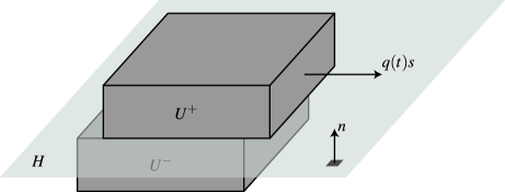
Figure 1. A microscopic slip.

Hence, the corresponding simple slip $\gamma_{t}\colon U\to\mathbb{R}^{d}$ expressing the deformation after time $t\geq 0$ is

$$\gamma_{t}(x)=\begin{cases}x&\text{if $x\in U^{-}$,}\\ x+\biggl{(}\displaystyle\int_{0}^{t}q(\tau)\;\mathrm{d}\tau\biggr{)}s&\text{if $x\in U^{+}$.}\end{cases}$$

If such a simple slip was to occur in a macroscopic state, it would be called a shear band, i.e. a shear motion over an infinitely thin plane, but we here assume it takes place on a microscopic scale and might not be visible macroscopically.

The space derivative of $\gamma_{t}$ in the BV-sense is the matrix-valued measure

$$\mathrm{D}\gamma_{t}=I\,\mathcal{L}^{d}+\biggl{(}\int_{0}^{t}q(s)\;\mathrm{d}s\biggr{)}s\otimes n\,\mathcal{H}^{d-1}\begin{picture}(10.0,8.0)\put(2.0,0.0){\line(0,1){7.0}}\put(1.8,0.0){\line(1,0){7.0}}\end{picture}H,$$

where $\mathcal{L}^{d}$ is the $d$-dimensional Lebesgue measure (the ordinary $d$-dimensional volume) and $\mathcal{H}^{d-1}\begin{picture}(10.0,8.0)\put(2.0,0.0){\line(0,1){7.0}}\put(1.8,0.0){\line(1,0){7.0}}\end{picture}H$ denotes the $(d-1)$-dimensional Hausdorff measure (the $(d-1)$-dimensional area) on $H$ and $I$ is the $d\times d$ identity matrix. Consequently, $\gamma_{t}$ is a (special) function of bounded variation. We refer to [13, 2] for information on this important class of functions and to [49] for a justification of the Kröner–Lee decomposition based on a similar argument.

A “differentiated” view on this simple slip is the following: For the plastic distortion $P(t)=\mathrm{D}\gamma_{t}$ (here there is no elastic distortion), we may derive the following differential equation:

$$\left\{\begin{aligned} \dot{P}(t)&=P(t)\bigl{[}q(t)s\otimes n\,\mathcal{H}^{d-1}\begin{picture}(10.0,8.0)\put(2.0,0.0){\line(0,1){7.0}}\put(1.8,0.0){\line(1,0){7.0}}\end{picture}H\bigr{]},\qquad t>0,\\ P(0)&=I,\end{aligned}\right.$$

which we understand as

$$\left\{\begin{aligned} \dot{P}(t,x)&=0&&\text{for $\mathcal{L}^{d}$-almost every $x\in\Omega$ and $t>0$,}\\ \dot{P}(t,x)&=P(t,x)[q(t)s\otimes n]&&\text{$(\mathcal{H}^{d-1}\begin{picture}(10.0,8.0)\put(2.0,0.0){\line(0,1){7.0}}\put(1.8,0.0){\line(1,0){7.0}}\end{picture}H)$-almost every $x\in\Omega$ and $t>0$,}\\ P(0,x)&=I&&\text{$(\mathcal{L}^{d}+\mathcal{H}^{d-1}\begin{picture}(10.0,8.0)\put(2.0,0.0){\line(0,1){7.0}}\put(1.8,0.0){\line(1,0){7.0}}\end{picture}H)$-almost every $x\in\Omega$.}\end{aligned}\right.$$

In particular, at every time $t>0$, a material vector $m$ from the tangent space to $U$ at a point in $H$ is changed with the rate

$$\dot{P}(t)m=q(t)(n\cdot m)P(t)s.$$

Notice that the referential vector $s$ is transformed into a “structural” vector $P(t)s$. This corresponds to the assumption that the slip direction $s$ is given with respect to the material frame, which is also natural since the hyperplane $H$ is specified in the material frame (there are no “structural points” as detailed below) and we need $s\perp n$. However, it is also possible to construct a “structural” formulation, but this leads to an equivalent theory, see Section 3.7.

The above linear matrix differential equation can be solved explicitly using the matrix exponential function (notice that in this special case all “generator” matrices $q(t)s\otimes n$ commute and $(s\otimes n)^{2}=0$ since $s\perp n$):

$$P(t) =\operatorname{Exp}(0)\,\mathcal{L}^{d}+\operatorname{Exp}\biggl{(}\int_{0}^{t}q(\tau)s\otimes n\;\mathrm{d}\tau\biggr{)}\,\mathcal{H}^{d-1}\begin{picture}(10.0,8.0)\put(2.0,0.0){\line(0,1){7.0}}\put(1.8,0.0){\line(1,0){7.0}}\end{picture}H$$

$$=I\,\mathcal{L}^{d}+\biggr{(}\int_{0}^{t}q(\tau)\;\mathrm{d}\tau\biggl{)}s\otimes n\,\mathcal{H}^{d-1}\begin{picture}(10.0,8.0)\put(2.0,0.0){\line(0,1){7.0}}\put(1.8,0.0){\line(1,0){7.0}}\end{picture}H$$

$$=D\gamma_{t},$$

as expected.

One can generalize the preceding discussion as follows: We postulate that also in the general situation, the plastic distortion $P(t)$ at time $t$ is given via the plastic distortion equation

$$\dot{P}=PD,$$ (2.1)

where $D$ is a $(d\times d)$-matrix field (or even a measure) called the (referential) plastic drift. In the case of the simple slip above,

$$D(t)=q(t)\,s\otimes n\,\mathcal{H}^{d-1}\begin{picture}(10.0,8.0)\put(2.0,0.0){\line(0,1){7.0}}\put(1.8,0.0){\line(1,0){7.0}}\end{picture}H.$$

In metals undergoing plastic distortion, $D$ arises from (activated) crystal defects that move around in the material, causing slip. Since $D$ by definition is a matrix in the referential frame, the equation (2.1) simply expresses that the referential drift, given by $D$, transformed to the plastically distorted configuration is equal to the change in the latter.

Example 2.1.

Often, one considers only plastic drifts $D$ that are a superposition of simple slips (for example all activated slip systems in crystal plasticity). All these slips have trace-free generators ($s\otimes n$ with $s\perp n$) and so in this case we require $D$ to be deviatoric:

$$\operatorname{tr}\,D=0.$$

From the general formula $\partial_{t}(\det\,A)=\det\,A\cdot\operatorname{tr}\,(A^{-1}\dot{A})$ and (2.1), we get

$$\partial_{t}(\det\,P)=\det\,P\cdot\operatorname{tr}\,D=0,$$

hence in this case the plastic incompressibility

$$\det\,P(t)=\det\,P(0)=1$$

holds.

It should be remarked that if $D$ is a sum of constant-in-time drifts (e.g. several different simple slips), $D=D_{1}+\cdots D_{n}$, then the evolution of $P$ is given as

$$P(t)=\operatorname{Exp}\bigl{(}(D_{1}+\cdots D_{n})t\bigr{)}P(0).$$

This, is however not equal to $\operatorname{Exp}(D_{1}t)\cdots\operatorname{Exp}(D_{n}t)P(0)$, because in general the matrices $D_{1},\ldots,D_{n}$ do not commute. To compute this expression, one would need to expand using the Baker–Campbell–Hausdorff formula, which involves the commutator brackets $[D_{k},D_{l}]$ ($k,l=1,\ldots,n$), see for example Chapter 3 in [20]. This simple observation already shows that due to the non-commutativity of drifts, we need to employ Lie group theory to make sense of the evolution of $P$.

If, as is common in much of the engineering literature (see for instance [19]), we instead worked with the structural drift $L=\dot{P}P^{-1}$, from (2.1) we have that

$$L=PDP^{-1},$$

so our $D$ is just the corresponding referential tensor for the structural tensor $L$.

2.2. Macroscopic kinematics

We now move from the microscopic to the macroscopic picture. Starting with an open, bounded reference configuration $\Omega\subset\mathbb{R}^{d}$ of material, we denote the referential (Lagrange, material) points in it as $x=(x^{1},\ldots,x^{d})\in\Omega$. Under an elasto-plastic deformation $y=(y^{1},\ldots,y^{d})\colon\Omega\to\mathbb{R}^{d}$, every referential point $x$ is mapped to a spatial (Euler) point $y=y(t,x)\in y(t,\Omega)$, where the time $t$ is from an interval $[0,T)$. A fundamental modeling assumption in this work (as in all of the continuum theory of plasticity) is the following:

Macroscopically, the elastically and plastically deformed body is again a continuum without interpenetration of matter or holes; thus $y(t)=y(t,\,\begin{picture}(1.0,1.0)(-0.5,-2.5)\circle*{2.0}\end{picture}\,)$ is a homeomorphism, that is, $y$ is continuous, bijective, and the inverse $y^{-1}$ is itself continuous.

For the sake of mathematical rigor we further assume that $y$ (and all other quantities) are as smooth as required, so we replace “homeomorphism” by “diffeomorphism” ($y$ and $y^{-1}$ continuously differentiable) in the previous assumption.

A referential vector $a\in\mathrm{T}_{x}\Omega$ at a referential point $x\in\Omega$, where $\mathrm{T}_{x}\Omega\cong\mathbb{R}^{d}$ denotes the tangent space to $\Omega$ at $x\in\Omega$, is transformed into a spatial vector $b\in\mathrm{T}_{y(t,x)}y(t,\Omega)$ via the push-forward

$$b=(\mathrm{d}y(t,x))_{*}a:=\nabla y(t,x)a,\qquad\text{where}\qquad\nabla y(t,x)=\left[\frac{\partial y^{j}}{\partial x^{k}}(t,x)\right]^{j}_{k}.$$

Note that here and in the following we switch between abstract vectors/co-vectors in the differential geometric sense and natural coordinates without further comment. Let us also adopt a simplifying notational convention: We leave out the arguments $t$ and $x$ to any quantity such as $y$ whenever this does not cause any confusion. So, we write $y$ instead of $y(t,x)$; the meaning should be clear from the context.

From physical reasoning we further require that no non-zero vector is mapped to the zero vector under the push-forward $\nabla y$ and that orientations are preserved. Hence, we require

$$\nabla y\in\mathrm{GL}^{+}(d),\qquad\text{i.e.,}\qquad\det\,\nabla y>0.$$

Fundamental to all geometrically nonlinear modeling in finite-strain elasto-plasticity is the multiplicative Kröner–Lee decomposition [25, 28, 27, 17, 5, 19, 49]

$$\nabla y=EP,$$

Here, $E$ and $P$ correspond to the elastic distortion and plastic distortion, respectively. The basic underlying assumption is that the plastic distortion is given as the “base” and the elastic distortion happens “on top of” the plastic distortion.

In general,

$$\operatorname{curl}E\neq 0\qquad\text{and}\qquad\operatorname{curl}P\neq 0,$$

whence we can only speak of $E,P$ as “distortions” (this terminology is from [19]) and not deformation gradients (there are no corresponding $y^{e},y^{p}$). We think of this in the following way: If $P$ is piecewise constant, everywhere except for the boundaries between different constancy domains, it is a local gradient of a piecewise-affine plastic deformation. However, the different affine pieces do not have to fit together without creating holes or overlaps. Since globally we assume that we end up with a continuum of mass again, these deformations have to be elastically corrected. Consequently, plastically distorted bodies sometimes cannot fully elastically unload: If $\operatorname{curl}P\neq 0$, then $E=I$ is impossible since otherwise we would have $\operatorname{curl}\nabla y=\operatorname{curl}(EP)\neq 0$, which is a contradiction.

In a more abstract fashion, we can consider there to be a vector bundle (see Chapter 10 of [29] for a formal definition) over the manifold $\Omega\times[0,+\infty)$, which we denote by $\mathrm{S}\Omega=(\mathrm{S}_{(t,x)}\Omega)_{t>0,x\in\Omega}$ and call the structural space, such that at every time $t>0$ and every point $x\in\Omega$ the associated vector space $\mathrm{S}_{(t,x)}\Omega:=\mathbb{R}^{d}$ contains the structural vectors. Then, the pushforward $(\mathrm{d}y(t,x))_{*}\colon\mathrm{T}_{x}\Omega\to\mathrm{T}_{y(t,x)}y(\Omega)$ splits into a plastic distortion $P\colon\mathrm{T}_{x}\Omega\to\mathrm{S}_{(t,x)}\Omega$ and an elastic distortion $E\colon\mathrm{S}_{(t,x)}\Omega\to\mathrm{T}_{y(t,x)}y(t,\Omega)$. The maps $P,E$ act on vectors in natural coordinates as multiplication with the respective matrices, also denoted by $P,E$. Sometimes, the engineering literature refers to the “structural (intermediate) configuration” between plastic and elastic distortions. This, however, can only be understood in the sense of transformation of vectors as before, but it is meaningless to transform points $x\in\Omega$ as there are no “structural points” (see Section 3.7 for more on this).

In our model, which is based on an explicit flow for the plastic part, $E$ only occurs as a derived quantity,

$$E=\nabla yP^{-1}.$$

Therefore, the issue of which invariances should be required of $E,P$, which is much discussed in the literature [17, 50, 35, 47, 9, 31, 46, 57, 5, 37], is not relevant here.

2.3. Local state spaces

The local state space contains all possible current states of the system at a given material point $x\in\Omega$. For the plastic distortion, we assume the existence of a real matrix Lie group $\mathfrak{P}\subset\mathrm{GL}^{+}(d)$ (that is, a group of matrices under matrix multiplication that is also a manifold such that multiplication and inversion are smooth operations), which we call the plastic distortion group, and require

$$P\in\mathfrak{P}.$$

Thus, the full signatures of $E,P$ are $E\colon[0,T)\times\Omega\to\mathrm{GL}^{+}(d)$ and $P\colon[0,T)\times\Omega\to\mathfrak{P}$, respectively. While the introduction of Lie group theory introduces some additional notation, it greatly clarifies some concepts and allows to consistently describe the signatures of many quantities occurring in the model.

In metals, plastic distortions are caused by the glide of microscopic dislocations, i.e. defects in the crystal structure of the material, see [26, 8, 23, 1, 53, 22] for some recent works in this direction. these are volume-preserving and so one often postulates plastic incompressibility

$$\det\,P=1.$$

In this case, $\mathfrak{P}\subset\mathrm{SL}(d)$.

Even the assumption of plastic incompressibility, however, still does not alleviate the so-called “uniqueness problem”: The Kröner–Lee decomposition $\nabla y=EP$ is far from unique except in very simple cases. We adopt the usual approach to treat $P$ as an internal variable and $E=\nabla yP^{-1}$ as a derived quantity.

We denote the Lie algebra associated with the Lie group $\mathfrak{P}$ by $\mathfrak{p}=\operatorname{Lie}(\mathfrak{P})$. Intuitively, elements of $\mathfrak{p}$ represent “infinitesimal” referential plastic distortion, or, more precisely, referential plastic rates, i.e. the speed by which a quantity changes. Formally, $\mathfrak{p}=\operatorname{Lie}(\mathfrak{P})$ can be defined as the tangent (vector) space to $\mathfrak{P}$ at the identity matrix, $\mathfrak{p}=\mathrm{T}_{I}\mathfrak{P}$. The fact that we consider the tangent space at the identity reflects the referential character of elements in $\mathfrak{p}$.

Example 2.2.

The following are some relevant Lie groups and Lie algebras:

• The Lie group $\mathfrak{P}=\mathrm{SL}(d)=\left\{\,A\in\mathbb{R}^{d\times d}\ \ \textup{{:}}\ \ \det\,A=1\,\right\}$, which has the Lie algebra $\mathfrak{p}=\mathfrak{sl}(d)=\left\{\,A\in\mathbb{R}^{d\times d}\ \ \textup{{:}}\ \ \operatorname{tr}\,A=0\,\right\}$, is the standard choice.

• If we choose $\mathfrak{P}=\mathrm{SO}(d)=\left\{\,A\in\mathbb{R}^{d\times d}\ \ \textup{{:}}\ \ A^{T}=A^{-1},\,\det\,A=1\,\right\}$ and $\mathfrak{p}=\mathfrak{so}(d)=\left\{\,A\in\mathbb{R}^{d\times d}\ \ \textup{{:}}\ \ A^{T}=-A\,\right\}$, then only orthogonal transformations are allowed, plastic shears are forbidden.

• A single slip system with slip direction $s\in\mathbb{R}^{d}$, $|s|=1$, and slip plane normal $n\in\mathbb{R}^{d}$, $|n|=1$ such that $s\perp n$ can be modeled using $\mathfrak{P}=\left\{\,I+\alpha(s\otimes n)\ \ \textup{{:}}\ \ \alpha\in\mathbb{R}\,\right\}$ and $\mathfrak{p}=\left\{\,\alpha(s\otimes n)\ \ \textup{{:}}\ \ \alpha\in\mathbb{R}\,\right\}$.

Motivated by the microscopic discussion about the plastic distortion equation, see (2.1), we define the (referential) plastic drift $\frac{\mathrm{D}}{\mathrm{D}t}P\colon[0,T)\times\Omega\to\mathfrak{p}$ (see below for the fact that $\frac{\mathrm{D}}{\mathrm{D}t}P\in\mathfrak{p}$) as

$$\frac{\mathrm{D}}{\mathrm{D}t}P:=P^{-1}\dot{P}.$$

To translate a spatial plastic distortion rate $\dot{P}\in\mathrm{T}_{P}\mathfrak{P}$ relative to the (plastically) deformed configuration to the referential frame, we need to pull it back to $\mathfrak{p}\cong\mathrm{T}_{I}\mathfrak{P}$. This is accomplished via a pre-multiplication of $\dot{P}$ with $P^{-1}$, yielding the referential plastic drift $\frac{\mathrm{D}}{\mathrm{D}t}P$. Thus, $\frac{\mathrm{D}}{\mathrm{D}t}P$ takes the role of $D$ in (2.1).

More abstractly, the elements of $\operatorname{Lie}(\mathfrak{P})$ can also be considered to be the left-invariant vector fields $X$ on $\mathfrak{P}$, that is $(\mathrm{d}L_{M})_{*}X=X$, where $L_{M}A:=MA$ is the left multiplication and $(dL_{M})_{*}$ its pushforward. Then we can express the pullback to the referential frame through $(\mathrm{d}L_{P^{-1}})_{*}\dot{P}=P^{-1}\dot{P}\in\mathfrak{p}$. Thus, the referential time derivative $\frac{\mathrm{D}}{\mathrm{D}t}$ acts on a curve $t\mapsto P(t)\in\mathfrak{P}$ as

$$\frac{\mathrm{D}}{\mathrm{D}t}P(t):=(\mathrm{d}L_{P(t)^{-1}})_{*}\frac{\mathrm{d}}{\mathrm{d}t}P(t)\quad\in\mathfrak{p}.$$ (2.2)

Note that taking the referential time derivative is not a linear operation, but it obeys the usual chain rule under reparametrizations.

The cotangent space $\mathrm{T}^{*}_{P}\mathfrak{P}$ to $\mathfrak{P}$ at $P$ contains stresses (forces per unit area), cf. [37]. An element $\sigma\in\mathrm{T}^{*}_{P}\mathfrak{P}$ can be pulled back to the cotangent space $\mathrm{T}^{*}_{I}\mathfrak{P}\cong\mathfrak{p}^{*}$ at the identity, where $\mathfrak{p}^{*}$ is the dual space to the Lie algebra $\mathfrak{p}$ (which is a Lie co-algebra, but we do not need this). This is accomplished via the map $\sigma\mapsto P^{T}\sigma\in\mathrm{T}^{*}_{I}\mathfrak{P}$, which can be checked by observing that

$$\dot{P}:\sigma=(P^{-1}\dot{P}):(P^{T}\sigma),$$

where $A:B:=\sum_{i,j}A^{i}_{j}B^{i}_{j}$ is the Frobenius product of the matrices $A,B\in\mathbb{R}^{d\times d}$, which here acts as the duality pairing between $\mathfrak{p}$ and $\mathfrak{p}^{*}$. The elements of $\mathfrak{p}^{*}$ therefore are referential stresses.

Furthermore, we assume that the material body possesses internal variables $z\in\mathfrak{Z}$, where $\mathfrak{Z}=\mathbb{R}^{m}$ is the canonical vector Lie group describing the internal variables of the system (for example, dislocation density in metals) with associated abelian (i.e. trivial) Lie algebra $\mathfrak{z}=\operatorname{Lie}(\mathfrak{Z})\cong\mathbb{R}^{m}$. General Lie groups $\mathfrak{Z}$ are also possible, but a simple vector will suffice for us here. According to (2.2), in this commutative Lie group we have for a curve $t\mapsto z(t)\in z(t)\in\mathfrak{Z}$ that

$$\frac{\mathrm{D}}{\mathrm{D}t}z(t)=\dot{z}(t).$$

since left “multiplication” is simply addition and hence $(\mathrm{d}L_{z(t)^{-1}})_{*}=\operatorname{id}$.

We bundle together the plastic distortion and internal variables (at a point) and define the (local) full internal state space as the product Lie group

$$\mathfrak{H}:=\mathfrak{P}\times\mathfrak{Z},$$

which has Lie algebra $\mathfrak{h}=\operatorname{Lie}(\mathfrak{H})\cong\mathfrak{p}\times\mathfrak{z}$, where $\mathfrak{p}=\operatorname{Lie}(\mathfrak{P})$ and $\mathfrak{z}=\operatorname{Lie}(\mathfrak{Z})$. In this way we consider the plastic distortion to be part of the internal state of the material, using the notation

$$H:=(P,z)\in\mathfrak{H}.$$

3. Energy and dissipation

In this section, we describe the energetics and basic dynamics of the two fundamental motions that we consider in our modelling approach: elastic minimization, for which $\dot{P},\dot{z}=0$, and elasto-plastic relaxation, for which $\dot{y}=0$. The next section will combine these basic motions into a full dynamic model, keeping in mind the relative speed by which these two motions progress.

3.1. Elastic free energy

The energetics of the material are governed by the free energy functional

$$\mathcal{W}[y,P,z]:=\int_{\Omega}W(x,\nabla y(t,x),P(t,x),z(t,x))\;\mathrm{d}x,$$

where $W\colon\Omega\times\mathrm{GL}^{+}(d)\times\mathfrak{H}\to\mathbb{R}$ is the energy density (recall $\mathfrak{H}=\mathfrak{P}\times\mathfrak{Z}$), which associates to each local state an energy per referential unit volume. We further split $W$ as

$$W(x,F,P,z)=W_{e}(x,FP^{-1})+W_{h}(x,z).$$

Here, $W_{e}\colon\Omega\times\mathrm{GL}^{+}(d)\to\mathbb{R}$ is the elastic energy density and $W_{h}\colon\Omega\times\mathfrak{Z}\to\mathbb{R}$ is the hardening energy density.

We assume $W_{e},W_{h}$ to be as smooth as necessary and $W_{e}$ to satisfy the objectivity (frame-indifference)

$$W_{e}(x,RE)=W_{e}(x,E)\qquad\text{for all $x\in\Omega$, $R\in\mathrm{SO}(d)$, $E\in\mathrm{GL}^{+}(d)$.}$$ (3.1)

Often, $W_{e},W_{h}$ also satisfy certain material symmetries, such as $W_{e}(x,ES)=W_{e}(x,E)$ for all $S$ from a symmetry group $\mathfrak{S}\subset\mathrm{GL}^{+}(d)$. The most common such material symmetry is isotropy, for which $\mathfrak{S}=\mathrm{SO}(d)$, the group of orthogonal $(d\times d)$-matrices with positive determinant, see Section 3.4 in [6]; a recent study of the isotropic case is in [16].

As already mentioned before, if $\operatorname{curl}P\neq 0$, no complete elastic unloading is possible, as $E\equiv R\in\mathrm{SO}(d)$ would then contradict $\operatorname{curl}EP=0$. Thus, not all of the free energy might be “free” to do work. However, as this is essentially a consequence of the requirement of geometric compatibility, we stick to the usual terminology.

With an external bulk loading $f(t,x)\in\mathbb{R}^{d}$ we also define the total energy functional

$$\mathcal{E}[t,y,P,z] :=\mathcal{W}[y,P,z]-\int_{\Omega}f(t,x)\cdot y(t,x)\;\mathrm{d}x$$

$$\phantom{:}=\int_{\Omega}W(x,\nabla y(t,x),P(t,x),z(t,x))-f(t,x)\cdot y(t,x)\;\mathrm{d}x.$$ (3.2)

3.2. The virtual power principle for purely elastic movements

Let $\Omega^{\prime}\subset\Omega$ be a referential subdomain of the body and denote by $n$ the unit outward normal on $\partial\Omega^{\prime}$. For the first fundamental motion of the system, namely the purely elastic motion, we assume $\dot{P}=0$, $\dot{z}=0$, which together with $\nabla y=EP$ implies

$$\dot{E}=\nabla\dot{y}P^{-1}.$$

Here and in the following we leave out the arguments $(t,x)$ to make the formulas more readable.

The internal power expended within $\Omega^{\prime}$ can be computed as

$$\mathcal{I}(\Omega^{\prime}) =\int_{\Omega^{\prime}}\frac{\mathrm{d}}{\mathrm{d}t}W(x,\nabla y,P,z)\;\mathrm{d}x$$

$$=\int_{\Omega^{\prime}}\mathrm{D}_{F}W(x,\nabla y,P,z):\nabla\dot{y}\;\mathrm{d}x$$

$$=\int_{\partial\Omega^{\prime}}\mathrm{D}_{F}W(x,\nabla y,P,z)n\cdot\dot{y}\;\mathrm{d}a+\int_{\Omega^{\prime}}-\operatorname{Div}[\mathrm{D}_{F}W(x,\nabla y,P,z)]\cdot\dot{y}\;\mathrm{d}x.$$

Notice that $\mathrm{D}_{F}W(x,F,P,z)\in\mathrm{T}^{*}_{F}\mathrm{GL}^{+}(d)$, which is the cotangent space to $\mathrm{GL}^{+}(d)$ at $F$; then, the Frobenius product “$:$” can also be interpreted as the application of this covector on the vector $\nabla\dot{y}$.

On the other hand, the external power expended on $\Omega^{\prime}$ is given by

$$\mathcal{P}(\Omega^{\prime})=\int_{\partial\Omega^{\prime}}t(n)\cdot\dot{y}\;\mathrm{d}a+\int_{\Omega^{\prime}}f(t)\cdot\dot{y}\;\mathrm{d}x-\int_{\Omega^{\prime}}\rho\ddot{y}\cdot\dot{y}\;\mathrm{d}x,$$

where $t(n)\in\mathbb{R}^{d}$ is the surface traction in direction $n$, $f(t)=f(t,x)\in\mathbb{R}^{d}$ is the external bulk loading and $\rho>0$ is the mass density. More complex external forces are of course possible as well, but we try to keep the exposition simple. Then, we assume the fundamental Principle of Virtual Power (see Chapter 92 in [19]):

The internal and external powers are equal, $\mathcal{I}(\Omega^{\prime})=\mathcal{P}(\Omega^{\prime})$, for all allowed choices of $(F,P,z)$ and all $\Omega^{\prime}\subset\Omega$.

In this context, $y$ and $E$ are referred to as virtual because they might not be attained in a given evolution (but they are attainable). Thus, with our $\mathcal{I}(\Omega^{\prime})$ and $\mathcal{P}(\Omega^{\prime})$, we get

$$\int_{\partial\Omega^{\prime}}\bigl{(}\mathrm{D}_{F}W(x,\nabla y,P,z)n-t(n)\bigr{)}\cdot\dot{y}\;\mathrm{d}a+\int_{\Omega^{\prime}}\bigl{(}\rho\ddot{y}-\operatorname{Div}[\mathrm{D}_{F}W(x,\nabla y,P,z)]-f\bigr{)}\cdot\dot{y}\;\mathrm{d}x$$

$$\qquad=0.$$

Then, since $\Omega^{\prime}\subset\Omega$ was arbitrary, we get the power balance (we drop the boundary equation since we do not need this information in the following)

$$\bigl{(}\rho\ddot{y}-\operatorname{Div}[\mathrm{D}_{F}W(x,\nabla y,P,z)]\bigr{)}\cdot\dot{y}=f\cdot\dot{y}.$$

The virtual rate $\dot{y}$ can attain any value, and so we conclude

$$\rho\ddot{y}-\operatorname{Div}[\mathrm{D}_{F}W(x,\nabla y,P,z)]=f.$$ (3.3)

Remark 3.1.

If we instead carry out the preceding computation for $W_{e}$, we get

$$\rho\ddot{y}-\operatorname{Div}[\mathrm{D}_{E}W_{e}(x,E)P^{-T}]=f.$$

However, it can be easily checked that $\mathrm{D}_{E}W_{e}(x,E)P^{-T}=\mathrm{D}_{F}W(x,\nabla y,P,z)$, and so this is the same as (3.3).

Besides the power balance expressed in the Principle of Virtual Power, we can also consider the balance of physical forces as fundamental. This gives rise to an alternative derivation of (3.3): The linear momentum of a (referential) subset $\Omega^{\prime}\subset\Omega$ is

$$\int_{\Omega^{\prime}}\rho\dot{y}\;\mathrm{d}x,$$

where $\rho>0$ is the density of the material.

By Newton’s Second Law, the change of linear momentum is equal to all forces acting on $\Omega^{\prime}$. There are two such forces:

1. The body force $\displaystyle\int_{\Omega^{\prime}}f\;\mathrm{d}x$.

2. The surface traction $\displaystyle\int_{\partial\Omega^{\prime}}t(n)\;\mathrm{d}a=\int_{\Omega^{\prime}}\operatorname{Div}T_{R}\;\mathrm{d}x=\int_{\Omega^{\prime}}\operatorname{Div}[\mathrm{D}_{F}W(x,\nabla y,P,z)]\;\mathrm{d}x$.

Thus, we have

$$\int_{\Omega^{\prime}}\rho\ddot{y}\;\mathrm{d}x=\frac{\mathrm{d}}{\mathrm{d}t}\int_{D}\rho\dot{y}\;\mathrm{d}x=\int_{\Omega^{\prime}}f+\operatorname{Div}[\mathrm{D}_{F}W(x,\nabla y,P,z)]\;\mathrm{d}x$$

As $\Omega^{\prime}\subset\Omega$ was arbitrary, this is equivalent to our previous force balance (3.3).

From now on we also assume (one can also derive a more complex theory without this):

Inertial forces can be neglected.

Then, we get the equilibrium equation

$$-\operatorname{Div}[\mathrm{D}_{F}W(x,\nabla y,P,z)]=f.$$

3.3. The virtual power principle for elasto-plastic relaxation movement

Now assume $\dot{y}=0$, whence on each subdomain $\Omega^{\prime}\subset\Omega$ the external power expended on $\Omega^{\prime}$ is zero. On the other hand, for the internal power we obtain

$$\mathcal{I}(\Omega^{\prime})=\int_{\Omega^{\prime}}\mathrm{D}_{P}W(x,\nabla y,P,z):\dot{P}+\mathrm{D}_{z}W(x,\nabla y,P,z)\cdot\dot{z}+X_{p}:\dot{P}+X_{z}\cdot\dot{z}\;\mathrm{d}x,$$

where

1. $X_{p}\colon\Omega\to T^{*}_{P}\mathfrak{P}$ is the generalized stress power-conjugate to $\dot{P}$ (recall that $T^{*}_{P}\mathfrak{P}$ is the cotangent space to $\mathfrak{P}$ at $P$, that is, the dual space to the tangent space $\mathrm{T}_{P}\mathfrak{P}$), and

2. $X_{z}\colon\Omega\to T^{*}_{z}\mathfrak{Z}$ is the generalized stress power-conjugate to $\dot{z}$.

The two generalized stresses $X_{p},X_{z}$ are the stresses that the system has to work against to deform plastically.

Since, again by the Principle of Virtual Power, $\mathcal{I}(\Omega^{\prime})=\mathcal{P}(\Omega^{\prime})=0$ for any subdomain $\Omega^{\prime}\subset\Omega$, we obtain the local balance of powers

$$\mathrm{D}_{P}W(x,\nabla y,P,z):\dot{P}+\mathrm{D}_{z}W(x,\nabla y,P,z)\cdot\dot{z}=-X_{p}:\dot{P}-X_{z}\cdot\dot{z}.$$ (3.4)

As $\dot{P}$ and $\dot{z}$ can take any value, we conclude the elasto-plastic relaxation balance

$$\left\{\begin{aligned} -\mathrm{D}_{P}W(x,\nabla y,P,z)&=X_{p}\\ -\mathrm{D}_{z}W(x,\nabla y,P,z)&=X_{z}.\end{aligned}\right.$$

Upon defining the referential plastic stress $T_{p}\colon\Omega\to\mathfrak{p}^{*}$ as

$$T_{p}:=-P^{T}\mathrm{D}_{P}W(x,\nabla y,P,z)$$

we can rewrite the elasto-plastic relaxation balance as

$$\left\{\begin{aligned} T_{p}&=P^{T}X_{p}\\ -\mathrm{D}_{z}W(x,\nabla y,P,z)&=X_{z}.\end{aligned}\right.$$ (3.5)

Since $\mathrm{D}_{P}W(x,\nabla y,P,z)\in\mathrm{T}^{*}_{P}\mathfrak{P}$, we indeed have $T_{p}(F,P,z)\in\mathfrak{p}^{*}$, see Section 2.3.

Let us also indicate how this rule can be written for $W_{e},W_{h}$ and the corresponding elastic stress: $T_{p}=-P^{T}\mathrm{D}_{P}W(x,\nabla y,P,z)$ lies in $\mathfrak{p}^{*}$, the dual space to $\mathfrak{p}$. In coordinates, we represent $\mathfrak{p},\mathfrak{p}^{*}$ by matrices and the duality product by the Frobenius product. Of course, $\mathfrak{p},\mathfrak{p}^{*}$ are in general strict subspaces of $\mathbb{R}^{d\times d}$, so there are additional conditions that have to be satisfied by matrices in these spaces. During coordinate calculations, these side constraints can become “lost” and so at the end we need to project onto the corresponding spaces again.

We have for any $D\in\mathfrak{p}$, and using $E:=\nabla yP^{-1}$,

$$T_{p}:D =-P^{T}\mathrm{D}_{P}W(x,\nabla y,P,z):D$$

$$=-\mathrm{D}_{P}W_{e}(x,E):(PD)$$

$$=\mathrm{D}_{E}W_{e}(x,E):[\nabla yDP^{-1}]$$

$$=\nabla y^{T}\mathrm{D}_{E}W_{e}(x,E)P^{-T}:D,$$

since for the derivative of $P\mapsto\nabla yP^{-1}$ in direction $PD\in\mathrm{T}_{P}\mathfrak{P}$, we have

$$\frac{\mathrm{d}(\nabla yP^{-1})}{\mathrm{d}P}[PD]=-\nabla yP^{-1}PDP^{-1}=-\nabla yDP^{-1}$$

by the well-known formula $\partial_{t}([A+tQ]^{-1})=-A^{-1}QA^{-1}$. Thus,

$$T_{p}=\mathrm{proj}_{\mathfrak{p}^{*}}\bigl{[}\nabla y^{T}\mathrm{D}_{E}W_{e}(x,E)P^{-T}\bigr{]},$$ (3.6)

where we denote the orthogonal projection onto $\mathfrak{p}^{*}$ by “$\mathrm{proj}_{\mathfrak{p}^{*}}$” (for example, if $\mathfrak{P}=\mathrm{SL}(d)$, $\mathfrak{p}=\mathfrak{sl}(d)$, then also $\mathfrak{p}^{*}\cong\mathfrak{sl}(d)$ and $\mathrm{proj}_{\mathfrak{p}^{*}}(U)=\operatorname{dev}U=U-(\operatorname{tr}U)I/d$).

We define the total generalized stress $\Sigma\colon\Omega\to\mathfrak{h}^{*}$ (recall that $\mathfrak{h}$ is the Lie algebra to $\mathfrak{H}$ and $\mathfrak{h}^{*}$ is its dual) through

$$\Sigma=\Sigma(x,F,P,z):=\bigl{(}T_{p}(x,F,P,z),-\mathrm{D}_{z}W(x,\nabla y,P,z)\bigr{)},$$ (3.7)

our balance (3.5) is then concisely expressed as

$$\Sigma=(P^{T}X_{p},X_{z}).$$ (3.8)

Finally, we remark that from the frame-indifference of $W$ by assumption (3.1), one may conclude that also $T_{p}$ is frame-indifferent, i.e.

$$T_{p}(RF,P,z)=T_{p}(F,P,z)\qquad\text{for all $R\in\mathrm{SO}(d)$.}$$

It is now straightforward to implement thermodynamic principles for the elasto-plastic relaxation phase by appealing to the free-energy imbalance as stated e.g. in Section 27.3 of [19], which is itself a consequence of the Second Law of Thermodynamics. The free-energy imbalance means that in each subregion $\Omega^{\prime}\subset\Omega$,

$$\frac{\;\mathrm{d}}{\;\mathrm{d}t}\mathcal{W}(\Omega^{\prime})-\mathcal{P}(\Omega^{\prime})=-\Delta(\Omega^{\prime})\leq 0,$$

with the nonnegative dissipation $\Delta(\Omega^{\prime})$. By the Principle of Virtual Power we also have $\mathcal{P}(\Omega^{\prime})=\mathcal{I}(\Omega^{\prime})$. Thus we obtain

$$\frac{\;\mathrm{d}}{\;\mathrm{d}t}\mathcal{W}(\Omega^{\prime})-\mathcal{I}(\Omega^{\prime})=-\Delta(\Omega^{\prime})\leq 0.$$

Since we are considering the elasto-plastic relaxation phase, $\nabla\dot{y}=0$. Then, use

$$\frac{\;\mathrm{d}}{\;\mathrm{d}t}W(x,\nabla y,P,z)=\mathrm{D}_{P}W(x,\nabla y,P,z):\dot{P}+\mathrm{D}_{z}W(x,\nabla y,P,z)\cdot\dot{z}$$

together with (3.4) and localize, which yields

$$X_{p}:\dot{P}+X_{z}\cdot\dot{z}=\delta\geq 0,$$

where $\delta\colon[0,T)\times\Omega\to[0,+\infty)$ is the dissipation rate. Then, using (3.8), we have for the component-wise scalar product $\Sigma\circ\frac{\mathrm{D}}{\mathrm{D}t}H$ that

$$\frac{\mathrm{D}}{\mathrm{D}t}H\circ\Sigma=\frac{\mathrm{D}}{\mathrm{D}t}P:(P^{T}X_{p})+\dot{z}\cdot X_{z}=\dot{P}:X_{p}+\dot{z}\cdot X_{z}=\delta\geq 0.$$ (3.9)

Inequality (3.9) expresses the irreversibility of plastic flow whenever $\delta>0$. In contrast, purely elastic deformations are of course reversible.

3.4. Dissipation potential and flow rule

So far we have not constitutively specified $X_{p}$ and $X_{z}$ in (3.8). In fact, we prefer – as is usual in much of the mathematical treatment of elasto-plasticity – to assume that (3.8) can be written as a differential inclusion or, equivalently, as a variational inequality. This is chiefly a structural assumption, in this context see Section 4.4 in [15] as well as [58, 54, 37]. At this point we just consider the situation in general and do not make any further assumptions (rate-dependence or rate-independence).

So, assume we have a dissipation (pseudo)potential $R\colon\mathfrak{h}\to[0,+\infty]$ (recall that $\mathfrak{h}=\mathfrak{p}\times\mathfrak{z}$) with the properties

$R$ is convex, lower semicontinuous, and strictly positive.

Here, strict positivity means that $R(\Lambda)\circ\Lambda>0$ for $\Lambda\neq 0$ (which is equivalent to $R(\Lambda)>0$ for $\Lambda\neq 0$ whenever $R$ is positively homogeneous of any order).

We furthermore assume that the flow rule (3.8) can be written in the form of the Biot inclusion (cf. Section 4.4 in [15] and [54])

$$\Sigma\in\partial R\biggl{(}\frac{\mathrm{D}}{\mathrm{D}t}H\biggr{)},\qquad\text{where}\qquad\frac{\mathrm{D}}{\mathrm{D}t}H:=\biggl{(}\frac{\mathrm{D}}{\mathrm{D}t}P,\frac{\mathrm{D}}{\mathrm{D}t}z\biggr{)}=(D,\dot{z})\in\mathfrak{h}.$$ (3.10)

Here, $\frac{\mathrm{D}}{\mathrm{D}t}H$ is called the total drift and $\partial$ denotes the convex subdifferential of $R$ at $\frac{\mathrm{D}}{\mathrm{D}t}H$, that is, $\partial R\bigl{(}\frac{\mathrm{D}}{\mathrm{D}t}H\bigr{)}$ consists of all those flow stresses $\Sigma\in\mathfrak{h}^{*}$ that satisfy

$$R\biggl{(}\frac{\mathrm{D}}{\mathrm{D}t}H\biggr{)}+\biggl{(}\Lambda-\frac{\mathrm{D}}{\mathrm{D}t}H\biggr{)}\circ\Sigma\leq R(\Lambda)\qquad\text{for all $\Lambda\in\mathfrak{h}$,}$$

where “$\circ$” is the component-wise scalar product between $\mathfrak{h}$ and $\mathfrak{h}^{*}$, that is, for $\Lambda=(A,c)\in\mathfrak{h}$ and $\Gamma=(B,d)\in\mathfrak{h}^{*}$ we have $\Lambda\circ\Gamma:=A:B+c\cdot d$.

If we for the moment (and for the purpose of illustration only) assume that our dissipation potential $R$ is differentiable, then the flow rule (3.10) expresses that

$$\Sigma=(T_{p},-\mathrm{D}_{z}W(x,\nabla y,P,z))=(P^{T}X_{p},X_{z})=\mathrm{D}R\biggl{(}\frac{\mathrm{D}}{\mathrm{D}t}H\biggr{)},$$

which is just (3.8) in a special form. In particular, we assume convexity and lower semicontinuity of $R$, which are not present in (3.8). If $R$ is positively $k$-homogeneous, then convexity of $R$ expresses the following intuitive constraint: When the system is moving in direction $\Lambda=(1-\theta)\Lambda_{0}+\theta\Lambda_{1}\neq 0$, where $\Lambda_{0},\Lambda_{1}\in\mathfrak{h}\setminus\{0\}$, $\theta\in(0,1)$, then the frictional power is $\mathrm{D}R(\Lambda)\circ\Lambda=kR(\Lambda)$ (by Euler’s positive homogeneity theorem); alternatively, we could oscillate very quickly between rates $\Lambda_{0},\Lambda_{1}$ with time-fractions $1-\theta$ and $\theta$, respectively, which would result in the frictional power $(1-\theta)kR(\Lambda_{0})+\theta kR(\Lambda_{1})$. The convexity tells us that this oscillatory path expends more energy, as should intuitively be the case for “reasonable” materials. Moreover, it can be shown that the Maximum Plastic Work Principle, which is a strengthening of the Second Law of Thermodynamics, implies convexity of $R$, see p. 57–59 in [21]. The lower semicontinuity is a minimal continuity assumption and can again be justified on physical grounds or out of mathematical necessity. Finally, the strict positivity means that energy is dissipated if and only if the material deforms plastically.

Note that in many applications $R$ does not depend on the state variables $(y,P,z)$ since we can often model changes in the size or shape of the elastic stability domain (defined below) through residual stresses. However, one may extend the theory to incorporate this constraint as well, but chose not to do this here for the sake of notational clarity.

The reason we specify the (primal/dual) flow rule in terms of the drift $(D,\dot{z})$ and not in terms of the current flow velocity $(\dot{P},\dot{z})$ is that when the material flows, the flow rule needs to “flow with the material”, and therefore $\frac{\mathrm{D}}{\mathrm{D}t}H$ ought to be a referential (or structural) quantity. Also see Section 3.7 for more on this.

Finally, define the dual dissipation potential $R^{*}\colon\mathfrak{h}^{*}\to[0,+\infty]$ as the convex conjugate function of $R$, that is,

$$R^{*}(\Sigma):=\sup\,\bigl{\{}\,\Sigma\circ\Lambda-R(\Lambda)\ \ \textup{{:}}\ \ \Lambda\in\mathfrak{h}\,\bigr{\}}.$$

Then, by standard results in convex analysis, see for example [52], we have that $R^{*}$ is also convex and lower semicontinuous. Moreover, the flow rule (3.10) is equivalent to the dual flow rule, which is sometimes called the Onsager inclusion,

$$\frac{\mathrm{D}}{\mathrm{D}t}H\in\partial R^{*}(\Sigma).$$ (3.11)

See [21] for more on these duality aspects, albeit in a geometrically linear framework.

So far, we have not specified anything about the dependence of $R$ on $\frac{\mathrm{D}}{\mathrm{D}t}H$ beyond convexity and lower semicontinuity and in fact we will later use several dissipation potentials.

According to the Coleman–Noll procedure [7, 18, 19], thermodynamic reasoning should give constitutive restrictions. In this spirit, combining (3.9) with the flow rule (3.10) yields the positivity condition on the dissipation potential $R$ and its dual $R^{*}$:

$$\frac{\mathrm{D}}{\mathrm{D}t}H\circ\partial R\biggl{(}\frac{\mathrm{D}}{\mathrm{D}t}H\biggr{)}\geq 0,\qquad\partial R^{*}(\Sigma)\circ\Sigma\geq 0$$ (3.12)

where the product “$\circ$” is understood to act on every stress in $\partial R\bigl{(}\frac{\mathrm{D}}{\mathrm{D}t}H\bigr{)}$ individually. This is a weaker version of the strict positivity we required above. Furthermore, it is elementary to see that for a convex function $g\colon X\to[0,+\infty]$ with $g(0)=0$ it always holds that $\partial g(x)\cdot x\geq 0$, hence the above condition (3.12) is automatically satisfied for convex $R$, giving another reason to require convexity as a structural property.

Finally, for a (time-differentiable) process $u=(y,P,z)$ we define the (total) dissipation over an interval $[s,t]$ as

$$\operatorname{Diss}(u;[s,t]):=\int_{s}^{t}\delta(\tau)\;\mathrm{d}\tau=\int_{s}^{t}\frac{\mathrm{D}}{\mathrm{D}\tau}H(\tau)\circ\Sigma(\tau)\;\mathrm{d}\tau\geq 0.$$

We will later see how to define the dissipation for lower-regularity processes.

3.5. Elastic stability domain

It is a fundamental property of elasto-plastic processes that if the generalized stress $\Sigma$ lies in the interior of an elastic stability domain $\mathcal{S}\subset\mathfrak{h}^{*}$, then no plastic flow takes place. The thinking here is that below the stress threshold $\partial\mathcal{S}$, which is called the yield surface, no plastic slip can be activated. This is in very good agreement with experiments, see Chapter 5 in [30]. We assume

$$\mathcal{S}\subset\mathfrak{h}$$ is a closed convex neighborhood of the origin.

In a more elaborate model, we could let $\mathcal{S}$ depend on the current internal state $(P,z)\in\mathfrak{H}$, but this introduces additional complications (for instance, when the system moves toward $\mathcal{S}(P,z)$, this set may “move away” and we may never reach it). Many interesting models, however, model changes in the elastic stability domain through a residual plastic stress and we confine ourselves to this setup.

In the usual rate-independent plasticity theory, $\mathcal{S}=\partial R_{1}(0)$ for the rate-independent flow potential $R_{1}$, and it is furthermore assumed that $\Sigma$ can never leave $\mathcal{S}$ and plastic flow is allowed only if the stress lies on the yield surface, i.e. $\Sigma\in\partial\mathcal{S}$. We here diverge from this usual modeling and allow $\Sigma$ to be outside $\mathcal{S}$, at least for a very short time. This occurs if the elastic minimization selects a state $(F,P,z)$ with $\Sigma(F,P,z)\notin\mathcal{S}$. This state, however, is transient in the sense that the material will try to correct the situation by following an elasto-plastic relaxation path, which at the terminal point will restore $\Sigma\in\mathcal{S}$. As we allow this relaxation to occur with infinite speed relative to the global (slow) time, this relaxation action is not visible on the slow (global) timescale. However, if the system jumps to a far away state, then, on a “fast” time scale, the relaxation path is not contracted and should form part of the solution concept of our model.

Remark 3.2.

It should be noted that the projection in (3.6) is of great importance for the consistency of the theory developed here: It ensures that only the plastic part of the stress remains in $T_{p}$. This is important, because only this stress can possibly be corrected by plastic flow. To illustrate this, consider a state $P=I$, $E=\alpha I$, $\alpha\neq 1$ for $\mathfrak{P}=\mathrm{SL}(d)$ (and no internal variables). The material cannot decrease its elastic energy, say $W_{e}(x,E):=\frac{1}{2}|E|^{2}=\alpha^{2}/2$, through an elasto-plastic relaxation flow, since a rate in $\mathfrak{p}=\mathfrak{sl}(d)$ cannot change the determinant of $E$. Thus, in order to always end up with $\Sigma\in\mathcal{S}$ after the elasto-plastic relaxation, it needs to hold that for $E=\alpha I$, $\alpha\neq 1$ we have $T_{p}=0$. Indeed, while $\mathrm{D}_{E}W_{e}(x,E)=\alpha I$ is not zero, it still holds that $T_{p}=0$ thanks to the projection onto deviatoric matrices in (3.7).

Example 3.3.

The elastic deformation domain $\mathcal{D}(P,z)\subset\mathrm{GL}^{+}(d)$ is the preimage of the map taking the total deformation $F$ to a generalized stress $\Sigma$ while holding $P,z$ constant:

$$\mathcal{D}(x,P,z):=\bigl{\{}\,F\in\mathrm{GL}^{+}(d)\ \ \textup{{:}}\ \ \Sigma(x,F,P,z)\in\mathcal{S}\,\bigr{\}}.$$

It models the set of deformation gradients $\nabla y$ that can be attained by a stable state. Even when the elastic energy density $W_{e}$ is convex, the geometry of the elastic deformation domain can be very complex. In particular, it does not follow that the elastic deformation domain $\mathcal{D}$ is convex. Indeed, consider the following example (without internal variables): Let for an $0<\varepsilon<1/\sqrt{2}$ the elastic stability domain be

$$\mathcal{S}=\bigl{\{}\,G\in\mathbb{R}^{2\times 2}\ \ \textup{{:}}\ \ \text{$|G-\operatorname{diag}(x,x)|\leq\varepsilon$,\, $x\in[0,1]$}\,\bigr{\}},$$

which is closed, convex, and a neighborhood of $0$. Also let $W_{e}(x,E)=\frac{1}{2}|E|^{2}$. Then, according to (3.5),

$$\Sigma(F,P)=F^{T}\mathrm{D}_{E}W_{e}(x,E)P^{-T}=F^{T}EP^{-T}=(F^{T}F)[P^{T}P]^{-1}.$$

At $P=I$, the elastic deformation domain is

$$\mathcal{D}(I)=\bigl{\{}\,F\in\mathbb{R}^{2\times 2}\ \ \textup{{:}}\ \ \Sigma(F,I)\in\mathcal{S}\,\bigr{\}}=\bigl{\{}\,F\in\mathbb{R}^{2\times 2}\ \ \textup{{:}}\ \ F^{T}F\in\mathcal{S}\,\bigr{\}},$$

which is not convex: the matrices $\operatorname{diag}(-1,1)$ and $\operatorname{diag}(1,1)$ are in $\mathcal{D}(I)$, but their average $\operatorname{diag}(0,1)$ is not, as a simple calculation shows.

3.6. Hardening

In its most general form, hardening describes the process by which the effective elastic stability domain changes, in particular expands or contracts, due to a change in the internal variables. Hardening is usually anisotropic and is due to a variety of microscopic effects like dislocation entanglement and generation.

In isotropic hardening, the elastic stability domain $\mathcal{S}$ remains centered around the origin but can expand in what is called positive hardening and contract in negative hardening or softening. In kinematic hardening, the elastic stability domain is translated (usually in direction of the plastic flow). Combined, these two effects give a first approximation to the often-observed phenomenon that an increase in tensile yield strength goes along with a decrease in compressive yield strength, called the Bauschinger effect, which, however, in general is more complex, see for instance Section 3.3.7 in [30] and [24].

Example 3.4.

In the often-considered Mises isotropic–kinematic hardening, the elastic stability domain depends on two internal variables, $S\in\mathfrak{p}^{*}\subset\mathbb{R}^{d\times d}$ and $\eta\in\mathbb{R}$, so that $\mathfrak{Z}=\mathfrak{p}^{*}\times\mathbb{R}$ (considered as a vector in $\mathbb{R}^{d^{2}+1}$). Then, the elastic stability domain is

$$\mathcal{S}=\Bigl{\{}\,\Gamma=(T_{p},S,\eta)\in\mathfrak{h}^{*}\ \ \textup{{:}}\ \ |\operatorname{dev}(T_{p}-S)|+\eta-\textstyle\frac{2}{3}\sigma_{0}\leq 0\,\Bigr{\}},$$

where $\sigma_{0}>0$ is a constant (the initial tensile yield strength) and $|A|=|A|_{F}=[\operatorname{tr}(A^{T}A)]^{1/2}$ is the Frobenius norm. The internal variables split into $S\in\mathfrak{p}^{*}$ and $\eta\in\mathbb{R}$, called backstresses. This means that the elastic stability domain is translated with $S$ and dilated with $\eta$ (a scalar stress). For the hardening energy $W_{h}$ we set (for instance)

$$W_{h}(S,\eta):=\frac{1}{2}g(|S|^{2})+h(\eta),$$

with $g,h\colon\mathbb{R}\to\mathbb{R}$ such that $g(0)=h(0)=0$. Notice that our $\mathcal{S}$ above does not depend on the internal variables $S,\eta$, which is characteristic for the approach using backstresses. In fact, a dependence of $\mathcal{S}$ on the internal variables seems to be needed only rarely. In purely isotropic hardening the internal variable $S$ is not present. Using a different matrix norm, one can get different shapes of the yield surface.

3.7. Referential versus structural formulation

There is some disagreement in the literature over what should be called the “undistorted” crystal lattice, see for example Section 91.2 in [19] and [46]. Of course, the observed lattice (which can be visualized for example through orientation-imaging microscopy) is the one that is already plastically distorted from the original referential lattice, so it is located in the structural space $\mathrm{S}\Omega$ defined in Section 2.3. We can always transform between referential and structural vectors by applying $P$, which gives the structural vector $Pm$ corresponding to a referential vector $m$, and the corresponding inverse transformation.

In mathematical terms, we need to decide whether we should formulate the flow rule and all other plastic quantities with respect to the reference frame or with respect to the structural frame, where the latter appears to be more popular [37, 19]. All quantities have versions in both frames. Indeed, in the structural frame, the plastic rate is measured via the structural plastic distortion rate

$$L:=\dot{P}P^{-1}=P\biggl{(}\frac{\mathrm{D}}{\mathrm{D}t}P\biggr{)}P^{-1},$$

which is a tensor that maps structural vectors to structural vectors since $P$ maps material vectors to structural vectors. The “structural stress” is the Mandel stress

$$M_{e}:=P^{-T}T_{p}P^{T}=-\mathrm{D}_{P}W(x,\nabla y,P,z)P^{T}.$$

It is easy to see that $L$ and $M_{e}$ are again conjugate in the sense that $M_{e}:L$ is equal to the dissipation $\delta$, in complete analogy to the fact that $T_{p}$ and $D$ are conjugate. Furthermore, it turns out that the referential and the structural flow rule are equivalent if $R$ is allowed to depend on $P$. Indeed, a computation shows that (3.10) is equivalent to

$$(M_{e},-\mathrm{D}_{z}W(x,\nabla y,P,z))\in\partial_{(L,\dot{z})}\tilde{R}(P,z,L,\dot{z}),$$

where

$$\tilde{R}(P,z,G,\zeta):=R(P^{-1}GP,\zeta).$$

Considering the abstract algebraic structure, the transition from referential to structural space is accomplished via conjugation: Define the adjoint mapping $\operatorname{Ad}_{Q}\colon\mathfrak{p}\to\mathfrak{p}$ and the dual adjoint mapping $\operatorname{Ad}^{*}_{Q}\colon\mathfrak{p}^{*}\to\mathfrak{p}^{*}$ through

$$\operatorname{Ad}_{Q}(A):=QAQ^{-1},\qquad\operatorname{Ad}^{*}_{Q}(A):=Q^{-T}AQ^{T}.$$

Then,

$$L=\operatorname{Ad}_{P}\biggl{(}\frac{\mathrm{D}}{\mathrm{D}t}P\biggr{)},\qquad M_{e}=\operatorname{Ad}^{*}_{P}(T_{p}).$$

Since $\operatorname{Ad}_{P}$ and $\operatorname{Ad}^{*}_{P}$ are isomorphisms, the formulations are indeed completely interchangeable. In the isotropic case, also $R=\tilde{R}$, see [16].

We remark that while the referential and the structural formulation are in principle equivalent, there may be good reasons to choose one over the other, at least in the non-isotropic case. It is quite possible that one of the $R,\tilde{R}$ is independent of $P$, whereas the other is not. In fact, if the anisotropy originates in the crystal lattice (for example different behavior along the crystal vectors in crystal plasticity), then the structural $\tilde{R}$ has a good chance of being independent of $P$ (and hence “simpler”). In this case, the whole model should be formulated in the structural frame, which is an easy translation. On the other hand, if the anisotropy is due to mesoscale laminations, then $R$ may be independent of $P$.

In the absence of the reasons just alluded to, we however believe that there is at least an “aesthetic” reason to prefer formulating the model in the reference frame: Since $P$ is in general not a gradient, there are no “structural points”, only material points. The engineering literature sometimes considers points $x_{S}$ in an imaginary “structural space”, but this is not a rigorous notion. Moreover, if we do not require the plastic incompressibility $\det P=1$ (soils, for example, are plastically compressible), which in any case should be treated as just a constitutive assumption, then the Mandel stress should reflect this and we really ought to use

$$M_{e}^{S}(x_{S}):=J_{p}(x_{R})P(x_{R})^{-T}T_{p}(x_{R})P(x_{R})^{T}\qquad\text{with}\qquad J_{p}(x_{R}):=\det P(x_{R}).$$

In other words, the points $x_{S}$ from the structural space are just points in $\Omega$, but the structural manifold $\Omega$ is now equipped with a different metric. All of this seems rather cumbersome and in light of the equivalence exposed above and also the microscopic motivation of plastic flow in (2.1), we prefer to work in the referential frame.

4. Global time evolution

In reality, plastic flow is rate-dependent (viscous), but only slightly so below absolute temperatures of approximately $0.35\vartheta_{m}$, where $\vartheta_{m}$ is the melting temperature of the material, see Section 78 in [19]. For instance, in a commonly-used power viscosity law (see Section 5.4 in [30]) the stress depends on the rate with exponent $1/N$, that is, $\mathrm{D}R(\Lambda)\sim|\Lambda|^{1/N}$. For example, steel with 35% carbon at 450 °C has $N=15$ and the titanium-aluminium alloy TA6V at 350 °C has $N=120$; more values can be found in Table 6.2 of [30]. The movement of the system is directed in such a way as to move the stress $\Sigma$ toward $\partial\mathcal{S}$, where the movement stops as the internal friction stress threshold is no longer exceeded. It can be seen that the larger $N$ is, the faster this “relaxation” takes place. Indeed, from the dual flow rule (3.11) we have $\frac{\mathrm{D}}{\mathrm{D}t}H=\mathrm{D}R^{*}(\Lambda)\sim|\Lambda|^{N}$. For $N\to\infty$, we approach “infinitely fast” relaxation.

On “slow” time scales we should therefore see near-infinitely fast relaxation, i.e. $\Sigma\in\mathcal{S}$ always, this is called (local) stability. In order to make this precise we will consider a time rescaling and pass to the limit (this is equivalent to letting $N\to\infty$). Then, for the resulting global evolution, we obtain a rate-independent evolution, at least where the solution process is continuous. This means that the system does not have any dynamics of its own and is purely driven by external forces.

However, it turns out that realistic concepts of solutions to rate-independent systems [45, 44, 56, 40, 41] must allow the system to jump from one state to another instantaneously (with respect to the slow global time scale). A key question, which is also central in other recent works [36, 37, 40, 41, 10, 11], is whether during a jump at “infinite” speed the modeling assumption of rate-independence can be upheld. Most materials in fact display rate-dependent behavior under fast deformations and this should be reflected in the modeling.

In a way opposite to the usual approach of starting with a rate-independent flow rule and then additionally specifying what happens during fast jumps, our strategy conversely starts with a rate-dependent flow rule and rescales time so that the slow (global) evolution becomes rate-independent wherever it is continuous, but during fast jumps the flow can be rate-dependent, rate-independent or a mixture of both. Thus, our model has two time parameters and hence we call our solutions two-speed solutions. Consequently, we posit the following key assumption:

The basic flow rule is rate-dependent, i.e. the fundamental dissipation potential $R$ is super-linear in the rate.

In order to arrive at a full evolutionary model, we consider the evolution to be partitioned into segments of equal duration and describe the dynamics as we step from one time point to the next. Here, we use the two fundamental motions (purely elastic minimization and elasto-plastic relaxation) described in the previous section. In order to combine them, we make the following fundamental assumption:

Elastic deformations are much faster than plastic flow. Equivalently, there is infinitesimal plastic inertia.

This is verified quite well experimentally, see for example [3, 4] and is also theoretically consistent (at least for metals) since the flow of dislocations is constricted to be always slower than the propagation of elastic deformation through shear waves (S-waves). This is so because the plastic drag tends to infinity as the plastic distortion rate approaches the shear wave speed, see [12].

Our time-stepping scheme then progresses by alternating between the following two stages:

1. Elastic minimization: When the material is moved out of elastic equilibrium, it first deforms in a purely elastic fashion, where the elastic distortion jumps (instantaneously) to a minimizer of the elastic energy, completely ignoring any plastic flow effects. Consequently, there may be an elastic excess, where the stress is outside the elastic stability domain, i.e. the constitutively specified stress region where the system cannot plastically flow (see below). We will use the Principle of Virtual Power (or, alternatively, a balance of forces) under the assumptions $\dot{P}=0$, $\dot{z}=0$ to derive the elastic force balance.

2. Elasto-plastic relaxation: To correct the elastic excess if it exists, the material then relaxes through an elasto-plastic flow, which is purely internal in the sense that the observable macroscopic shape of the body remains the same, i.e., $\dot{y}=0$. Again via the Principle of Virtual Power we derive the elasto-plastic power balance and then the flow rule. The flow stops once the stress has reached the elastic stability domain.

This splitting of the motion into the above two basic modes is the defining feature of the present model and we consider it to be physically realistic (it is also somewhat reminiscent of predictor–corrector schemes in numerics). Another benefit is that it allows for a clean modeling. In this context notice that the elastic minimality from Stage I will potentially be destroyed by the relaxation in Stage II, and the condition that the stress is contained in the elastic stability domain might no longer hold true after a successive Stage I (even if the external loading does not change). Therefore, we really should iterate these stages until we have reached a fixed point. This, however, turns out not to be necessary, since we will perform both stages for each time step in a time-stepping problem and letting the time step size go to zero will have the same effect.

4.1. Fast flow rule

As outlined above, let $R\colon\mathfrak{h}\to[0,+\infty]$ be a given rate-dependent dissipation (pseudo)potential that we assume to be convex, lower semicontinuous, and superlinear, that is

$$\liminf_{|\Lambda|\uparrow\infty}\,\frac{R(\Lambda)}{|\Lambda|}=\infty.$$

Furthermore, for $\Gamma\notin\mathcal{S}$, we want to assume that $R^{*}(\Gamma)$ is continuously differentiable in $\Gamma$, expressing the fact that we model a deterministic system, i.e. that the flow direction and speed are uniquely determined. Then, also $R(\Lambda)$ is continuously differentiable for all $\Lambda$ such that $\Lambda=\mathrm{D}R^{*}(\Gamma)$ for some $\Gamma\notin\mathcal{S}$, see [52].

Note that additionally $R$ could depend on the current state $(\nabla y,H)\in\mathrm{GL}^{+}(d)\times\mathfrak{H}$, but we suppress this dependency for ease of notation.

As long as $\Sigma\notin\mathcal{S}$, plastic flow is governed by our flow rule

$$\Sigma\in\partial R\biggl{(}\frac{\mathrm{D}}{\mathrm{D}t}H\biggr{)}\quad\Longleftrightarrow\quad\frac{\mathrm{D}}{\mathrm{D}t}H\in\partial R^{*}(\Sigma),$$

see (3.10), (3.11). Additionally, we want to express the notion that the flow stops once we have reached the elastic stability domain $\mathcal{S}$. Thus, we really use the combined flow rule

$$\frac{\mathrm{D}}{\mathrm{D}t}H=\begin{cases}0&\text{if $\Sigma\in\mathcal{S}$,}\\ \mathrm{D}R^{*}(\Sigma)&\text{otherwise.}\end{cases}$$ (4.1)

Clearly, we only need the dual flow potential $R^{*}(\Sigma)$ for $\Sigma\notin\mathcal{S}$ since the flow stops once we have reached the yield surface $\partial\mathcal{S}$. Therefore, we now change notation slightly and from here onwards denote by $R\colon\mathfrak{h}\to[0,+\infty)$ the combined dissipation potential, for which we furthermore require the decomposition

$$R(\Gamma)=R_{1}(\Gamma)+R_{+}(\Gamma)$$ (4.2)

into the following two components:

1. $R_{1}\colon\mathfrak{h}\to[0,+\infty)$ is the rate-independent dissipation potential, which is equal to the support function of $\mathcal{S}$,

   $$\qquad R_{1}(\Lambda)=\sigma_{\mathcal{S}}(\Lambda):=\sup_{\Gamma\in\mathcal{S}}\Lambda\circ\Gamma,$$

   i.e. the dual of the characteristic function $\chi_{\mathcal{S}}$ of $\mathcal{S}$ (which is $0$ on $\mathcal{S}$ and $+\infty$ otherwise).

2. $R_{+}\colon\mathfrak{h}\to[0,+\infty)$ is the convex, differentiable residual dissipation potential. We also assume that its dual $R_{+}^{*}$ is strictly positive, that is $R_{+}^{*}(0)=0$ and $R_{+}^{*}(\Gamma)>0$ for $\Gamma\neq 0$ (this is essentially a superlinearity assumption on $R_{+}$ and for instance satisfied if $\liminf_{t\to 0}\,R_{+}(t\Lambda)/t=0$).

It turns out that the decomposition (4.2) implies

$$R^{*}(\Sigma)=\inf_{\Gamma\in\mathcal{S}}R_{+}^{*}(\Sigma-\Gamma).$$ (4.3)

Indeed, we can compute, using the inf-convolution $(f\operatorname{\square}g)(x):=\inf_{z}[f(x-z)+g(z)]$ and the associated duality rule $[f\operatorname{\square}g]^{*}=f^{*}+g^{*}$ (see Theorem 16.4 of [52]), that

$$R^{*}(\Sigma)=[R_{1}+R_{+}]^{*}(\Sigma)=[R_{1}^{*}\operatorname{\square}R_{+}^{*}](\Sigma)=\inf_{\Gamma\in\mathcal{S}}R_{+}^{*}(\Sigma-\Gamma).$$

In particular, using the strict positivity of $R_{+}^{*}$, we have for the dual combined dissipation potential $R^{*}\colon\mathfrak{h}^{*}\to[0,+\infty]$ the property that

$$R^{*}(\Sigma)=0\quad\text{if and only if}\quad\Sigma\in\mathcal{S}.$$

Consequently, $R^{*}$ by itself already determines $\mathcal{S}$ and the flow rule for our new $R$ is the combined flow rule (4.1).

On the other hand, assume that we are given $\mathcal{S}\subset\mathfrak{h}^{*}$ with $0\in\mathcal{S}$ and a convex, differentiable dual residual dissipation potential $R_{+}^{*}\colon\mathfrak{h}^{*}\to[0,+\infty)$ with the strict positivity property from above. Then, we can define $R^{*}$ (and hence by duality $R$) through (4.3) and we obtain for $R$ that

$$R=[R^{*}]^{*}=\bigl{[}\chi_{\mathcal{S}}\operatorname{\square}R_{+}^{*}\bigr{]}^{*}=R_{1}+R_{+}$$

where we have set $R_{1}:=\sigma_{\mathcal{S}}=\chi_{\mathcal{S}}^{*}$ and $R_{+}:=R_{+}^{**}:=[R_{+}^{*}]^{*}$. Thus, the decomposition above holds, where we also note that $R_{1}\geq 0$ because of $0\in\mathcal{S}$ and $R_{+}=R_{+}^{**}\geq 0$ because of $R_{+}^{*}(0)=0$.

4.2. Associative flow potentials

An important special case, which we discuss for further illustration, is a material that is associative. While there is considerable disagreement in the literature over what exactly constitutes an associative flow rule, we here understand it to mean that there exists a proper, lower semicontinuous, convex, and strictly increasing $\zeta_{+}^{*}\colon[0,+\infty)\to[0,+\infty)$ and a norm $\|\,\begin{picture}(1.0,1.0)(-0.5,-2.5)\circle*{2.0}\end{picture}\,\|_{+}^{*}$ on $\mathfrak{h}^{*}$ such that

$$R_{+}^{*}(\Gamma)=\zeta_{+}^{*}(\|\Gamma\|_{+}^{*}),\qquad\Gamma\in\mathfrak{h}^{*}.$$

The utility of these assumptions is that they allow to simplify the definition (cf. (4.3)) of the dual combined dissipation potential $R^{*}\colon\mathfrak{h}^{*}\to[0,+\infty)$ to

$$R^{*}(\Gamma)=\begin{cases}0&\text{if $\Gamma\in\mathcal{S}$,}\\ \zeta_{+}^{*}(\operatorname{dist}_{\|\,\begin{picture}(1.0,1.0)(-0.5,-2.5)\circle*{2.0}\end{picture}\,\|_{+}^{*}}(\Gamma,\mathcal{S})&\text{if $\Gamma\notin\mathcal{S}.$}\end{cases}$$

where $\operatorname{dist}_{\|\,\begin{picture}(1.0,1.0)(-0.5,-2.5)\circle*{2.0}\end{picture}\,\|_{+}^{*}}(\Gamma,\mathcal{S}):=\inf_{\Gamma^{\prime}\in\mathcal{S}}\|\Gamma-\Gamma^{\prime}\|_{+}^{*}$ is the distance function with respect to the norm $\|\,\begin{picture}(1.0,1.0)(-0.5,-2.5)\circle*{2.0}\end{picture}\,\|_{+}^{*}$. In this case, all flow rates are normal to the elastic stability domain, that is,

$$\partial R^{*}(\Gamma)\subset\mathrm{N}_{\mathcal{S}}(\Gamma)\qquad\text{for all $\Gamma\in\partial\mathcal{S}$.}$$

where $\mathrm{N}_{\mathcal{S}}(\Gamma)$ denotes the normal cone to $\mathcal{S}$ at $\Gamma\in\partial\mathcal{S}$, i.e.

$$\mathrm{N}_{\mathcal{S}}(\Gamma):=\bigl{\{}\,\Lambda\in\mathfrak{h}\ \ \textup{{:}}\ \ \text{$\Lambda\circ(\Gamma^{\prime}-\Gamma)\leq 0$ for all $\Gamma^{\prime}\in\mathcal{S}$}\,\bigr{\}}.$$

This is related to the Maximum Plastic Work Principle, which is a strengthening of the Second Law of Thermodynamics, see p. 57–59 in [21].

Example 4.1.

A common choice for a rate-dependent dissipation potential $R\colon\mathfrak{sl}(d)\to\mathbb{R}$ (recall that $\mathfrak{sl}(d)$ contains all trace-free $(d\times d)$-matrices), is a Mises power law, see for instance Section 101 in [19], that is, the restriction of

$$\hat{R}(V):=\frac{\kappa}{1+1/N}|V|^{1+1/N}$$

to the complement of the elastic stability domain

$$\mathcal{S}=\bigl{\{}\,V\in\mathfrak{sl}(d)^{*}\ \ \textup{{:}}\ \ \hat{R}^{*}(V)\leq\kappa/(1+N)\,\bigr{\}}=B_{\mathfrak{sl}(d)^{*}}(0,\kappa)\subset\mathfrak{sl}(d)^{*}.$$

Here, $\kappa>0$ and $N>1$. Since for $V\in\mathfrak{sl}(d)^{*}$,

$$\hat{R}^{*}(V)=\frac{\kappa}{1+N}\biggl{(}\frac{|V|}{\kappa}\biggr{)}^{1+N},$$

we may compute

$$R_{1}(V)=\sigma_{\mathcal{S}}(V)=\kappa|V|\qquad\text{and}\qquad R_{+}(V)=\kappa\biggl{[}\frac{|V|^{1+1/N}}{1+1/N}+\frac{1}{1+N}-|V|\biggr{]}^{+},$$

where $[s]^{+}=\max(s,0)$. Then, indeed $R|_{\mathfrak{sl}(d)\setminus\mathcal{S}}=\hat{R}|_{\mathfrak{sl}(d)\setminus\mathcal{S}}$.

4.3. Relaxation paths

Let $F_{0}\in\mathrm{GL}^{+}(d)$, $(P_{0},z_{0})\in\mathfrak{H}$ such that $\Sigma(F_{0},P_{0},z_{0})\notin\mathcal{S}$. Then the system is driven towards relaxation by following a relaxation path $\gamma\colon[0,\tau_{\gamma}]\to\mathfrak{H}$, where $\tau_{\gamma}>0$ may depend on the path $\gamma$, until relaxation is achieved when $\Sigma(F_{0},\gamma(\tau_{\gamma}))\in\partial\mathcal{S}$. We define $\gamma$ through

$$\left\{\begin{aligned} \gamma(0)&=(P_{0},z_{0}),\\ \frac{\mathrm{D}}{\mathrm{D}t}\gamma(t)&\in\partial R^{*}\bigl{(}\Sigma(F_{0},\gamma(t))\bigr{)},\quad t\in[0,\tau_{\gamma}),\\ \Sigma(F_{0},\gamma(t))&\notin\mathcal{S}\quad\text{for}\quad t\in[0,\tau_{\gamma}),\\ \Sigma(F_{0},\gamma(\tau_{\gamma}))&\in\partial\mathcal{S}.\end{aligned}\right.$$

Note that $\frac{\mathrm{D}}{\mathrm{D}t}\gamma=(\frac{\mathrm{D}}{\mathrm{D}t}P,\dot{z})$, where $\gamma(t)=(P(t),z(t))$.

Assuming that this path exists and is unique, we denote its endpoint by $Y(f_{0},P_{0},z_{0})$. If we also set $Y(F_{0},P_{0},z_{0}):=(P_{0},z_{0})$ if already $\Sigma(F_{0},P_{0},z_{0})\in\mathcal{S}$, then $Y$ can be considered a function $Y\colon\mathrm{GL}^{+}(d)\times\mathfrak{H}\to\mathfrak{H}$ with the property that

$$\Sigma(F_{0},Y(P_{0},z_{0}))\in\mathcal{S}\qquad\text{for all $(F_{0},P_{0},z_{0})\in\mathrm{GL}^{+}(d)\times\mathfrak{H}$.}$$

4.4. Time rescaling and time-stepping evolution

Conceptually, rate-independence is of course not a physical property of a system, but a mathematical rescaling limit. So, consider an elasto-plastic process $u(t)=(y(t),P(t),z(t))$ with external loading $f=f(t)$, where $t\in[0,T)$. Then, the basic assumption in this work is that the system evolves according to a (fast) flow rule as defined above. However, as discussed before, if $f$ were to be held constant at some point in time, the system would settle very quickly into a rest state until the external loading changes and the system is pushed out of equilibrium. The traditional rate-independent modeling is built upon the assumption that only this global movement is interesting and the fast “relaxation” movements towards a rest state can be neglected, at least if the system does not jump to a far-away state in an instant.

This idealized situation is mathematically expressed through rescaling: Define for small $\lambda>0$ the process $\tilde{u}_{\lambda}(\theta)$ as a solution of the fast dynamics for the slower external loading $\tilde{f}_{\lambda}(\theta)=f(\lambda\theta)$, where now $\theta\in[0,T/\lambda]$. It is, however, inconvenient to deal with changing time intervals and so we reparametrize the whole process by setting $u_{\lambda}(t):=\tilde{u}_{\lambda}(t/\lambda)$, $t\in[0,T)$. This has the effect of keeping the external loading at constant speed, but accelerating the response dynamics of the system by the factor $1/\lambda$.

Letting $\lambda\downarrow 0$, we call the limit process $u_{0}(t):=\lim_{\lambda\downarrow 0}u_{\lambda}(t)$ the rate-independent limit. It models the situation where the relaxation behavior of the system is infinitely fast and the system remains completely stationary if the external loading does not change. However, this acceleration is only due to a rescaling of time, which does not affect the dissipative energetics. So, effectively, this new system has a different (rescaled) dissipation law to reflect the rescaling in time. More concretely, the “fast” relaxation paths $\gamma_{\lambda}$ (corresponding to the $\gamma$’s from the previous section) for $u_{\lambda}$ have to modified to read

$$\lambda\frac{\mathrm{D}}{\mathrm{D}t}\gamma_{\lambda}(t)\in\partial R^{*}\bigl{(}\Sigma(F_{0},\gamma_{\lambda}(t))\bigr{)},\quad t\in[0,\lambda\tau_{\gamma}).$$

In the following we will develop an approximative, time-stepping, scheme whose solution reflects this sped-up response.

For reasons of consistency, we assume that the initial values $u_{\mathrm{start}}=(y_{\mathrm{start}},H_{\mathrm{start}})$ where the diffeomorphism $y_{\mathrm{start}}\colon\Omega\to\mathbb{R}^{d}$ and $H_{\mathrm{start}}\colon\Omega\to\mathfrak{H}$ constitute a rest state, i.e.

$$y_{\mathrm{start}}\quad\text{minimizes}\quad\hat{y}\mapsto\mathcal{E}[0,\hat{y},H_{\mathrm{start}}]\qquad\text{and}\qquad\Sigma(u_{\mathrm{start}})\in\mathcal{S}.$$

Here, recall the definition of $\mathcal{E}$ from (3.2). This condition is imposed to ensure that the system does not immediately jump and we should have chosen the endpoint of the jump as initial value.

Let $N\in\mathbb{N}$ and divide the time interval $[0,T)$ into an equidistant partition

$$0=t_{0}^{N}<t_{1}^{N}<\cdots<t_{2^{N}}^{N}=T,\qquad t_{k}=k2^{-N}T\quad\text{($k=0,\ldots,2^{N}$).}$$

We also need the rescaling coefficient $\lambda^{N}>0$, which describes the time-rescaling. We require that that $\lambda^{N}\downarrow 0$ as $N\to\infty$ “more slowly” than the partition, that is,

$$\lambda^{N}2^{N}\uparrow\infty\qquad\text{as $N\to\infty$.}$$

This constraint expresses that the elastic minimization is relatively faster than the elasto-plastic relaxation.

The time-stepping evolution $u^{N}=(y^{N},P^{N},z^{N})$ consists of the component functions $y^{N}\colon[0,T)\times\Omega\to\mathbb{R}^{d}$, $P^{N}\colon[0,T)\times\Omega\to\mathfrak{P}$, $z^{N}\colon[0,T)\times\Omega\to\mathfrak{Z}$. In every consecutive time period $[t_{k},t_{k+1})$ the discrete system in turn executes the following two stages (illustrated in Figure 2):

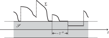
Figure 2. The two-stage time-stepping scheme.

1. Elastic minimization: First, we let the system deform elastically as if there was no plastic flow rule present. Let the diffeomorphism $y_{*}\colon\Omega\to\mathbb{R}^{d}$ be such that (holding $H^{N}(t_{k}):=(P^{N}(t_{k}),z^{N}(t_{k}))$ fixed)

   $$\qquad y_{*}\quad\text{minimizes}\quad\hat{y}\mapsto\mathcal{E}[t_{k},\hat{y},H^{N}(t_{k})]$$

   over all diffeomorphisms $\hat{y}\colon\Omega\to\mathbb{R}^{d}$ that also satisfy the prescribed boundary conditions. We assume that the system’s total deformation jumps immediately to $y_{*}$:

   $$\qquad y^{N}(t):=y_{*},\qquad t\in[t_{k},t_{k+1}).$$

2. Elasto-plastic relaxation: Whenever necessary, the system will now exchange elastic for plastic distortion to restore the requirement that the generalized stress lies within the elastic stability domain. We define the internal state at a fixed $x\in\Omega$ as

   $$\qquad H^{N}(t,x):=(P^{N}(t,x),z^{N}(t,x))\in\mathfrak{H},\qquad t\in[t_{k},t_{k+1}).$$

   Then, for the evolution of $H^{N}_{x}$ we consider two cases, depending on the value of $F_{0}:=\nabla y_{*}$:

   1. If $\Sigma(F_{0},H^{N}(t_{k},x))\in\mathcal{S}$, then set (no flow)

      $$\qquad\qquad H^{N}(t,x):=H^{N}(t_{k},x),\qquad t\in[t_{k},t_{k+1}).$$

   2. Otherwise, the system needs to relax through elasto-plastic flow, for which it employs a relaxation path $\gamma$ as in Section 4.3 with $F_{0}=\nabla y_{*}(x)=\nabla y^{N}(t_{k},x)$ (for our fixed $x$). Let $\gamma\colon[0,\tau_{\gamma}]\to\mathfrak{H}$ be the relaxation path starting at $H^{N}(t_{k},x)$, which we consider to be constantly extended to $\gamma\colon[0,+\infty)\to\mathfrak{H}$ and set

      $$\qquad\qquad H^{N}(t,x):=\gamma\biggl{(}\frac{t-t_{k}}{\lambda^{N}}\biggr{)},\qquad t\in[t_{k},t_{k+1}).$$

      Note that it is possible that, depending on the value of $\lambda^{N}$, the relaxation path may be shorter than the full interval (if $\tau_{\gamma}\lambda^{N}\leq 2^{-N}T$ ) or longer, in which case the relaxation is not complete by the next time point $t_{k+1}$. Furthermore, since we assumed that all relaxations are internal, during the relaxation the full deformation does not change. See Figure 3 for an illustration of the relaxation.

   Thus, we have the effective flow rule

   $$\qquad\qquad\Sigma(u^{N}(t,x))\in\partial R\biggl{(}\lambda^{N}\frac{\mathrm{D}}{\mathrm{D}t}H^{N}(t,x)\biggr{)},\qquad(t,x)\in(t^{N}_{k},t^{N}_{k+1})\times\Omega.$$

   Note that only if $\tau_{\gamma}\lambda^{N}\leq 2^{-N}T$, at the end of the relaxation path it holds that

   $$\qquad\Sigma(u^{N}(t_{k+1},x))\in\mathcal{S},$$

   hence the system has reached an elastically allowable state. Of course, in this process, $y^{N}(t_{k})$ does not necessarily retain the minimization property from stage (I).

We iterate this scheme for $k=1,\ldots,2^{N}$ and call the resulting $u^{N}=(y^{N},H^{N})$ the time-stepping evolution at level $N$.

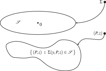
Figure 3. The elasto-plastic relaxation flow.

5. Limit passage and two-speed solutions

Assume we have a sequence of time-stepping solutions $u^{N}\colon[0,T)\times\Omega\to\mathbb{R}^{d}\times\mathfrak{H}$. In this section we will consider heuristics of the limit passage $N\to\infty$ in order to understand the continuous-time behavior. This can be seen as a “blueprint” of a future fully rigorous mathematical analysis. We do not state all the precise assumptions, but indicate key requirements as we go along.

As the basis of all of the following we require:

1. $\displaystyle u^{N}\to u_{0}=(y_{0},P_{0},z_{0})\colon[0,T)\times\Omega\to\mathbb{R}^{d}\times\mathfrak{H}$ in a sufficiently good sense.

This would have to be made precise in a rigorous treatment, we here simply assume that the convergence is “good enough” to make all the following arguments work.

We will distinguish two types of points $t_{0}\in[0,T)$: regular and singular points. At regular points, we assume the bound

$$\int_{\Omega}\biggl{|}\frac{\mathrm{D}}{\mathrm{D}t}H^{N}(x,t)\biggr{|}\;\mathrm{d}x\quad\text{is uniformly (in $N,t$) bounded for $t\in[t_{0}-\varepsilon,t_{0}+\varepsilon]$.}$$ (5.1)

Here, $\varepsilon>0$ may depend on $t_{0}$, but we suppress this in the notation. All other points are called singular points. Accordingly, at regular points the internal variables do not change too fast, whereas at singular points $u^{N}$ may develop a jump.

We start by making two preliminary observations: First, from the (fast) flow inclusion in the elasto-plastic relation stage,

$$\Sigma(u^{N}(t,x))\in\partial R\biggl{(}\lambda^{N}\frac{\mathrm{D}}{\mathrm{D}t}H^{N}(t,x)\biggr{)},\qquad(t,x)\in(t^{N}_{k},t^{N}_{k+1})\times\Omega,$$

we estimate for $\tau\in(t^{N}_{k},t^{N}_{k+1})$ that

$$-\frac{\mathrm{d}}{\mathrm{d}t}\mathcal{W}[u^{N}(t)] =\frac{1}{\lambda^{N}}\int_{\Omega}\Sigma(u^{N}(t))\circ\lambda^{N}\frac{\mathrm{D}}{\mathrm{D}t}H^{N}(t)\;\mathrm{d}x$$

$$=\frac{1}{\lambda^{N}}\int_{\Omega}R\biggl{(}\lambda^{N}\frac{\mathrm{D}}{\mathrm{D}t}H^{N}(t)\biggr{)}+R^{*}\bigl{(}\Sigma(u^{N}(t))\bigr{)}\;\mathrm{d}x$$

$$\geq\int_{\Omega}R_{1}\biggl{(}\frac{\mathrm{D}}{\mathrm{D}t}H^{N}(t)\biggr{)}\;\mathrm{d}x\geq 0.$$ (5.2)

Here we used that if $\Gamma\in\partial R(\Lambda)$, then $\Lambda\circ\Gamma=R(\Lambda)+R^{*}(\Gamma)$, this is Fenchel’s Theorem, see for instance Theorem 23.5 in [52] and $R_{+}\geq 0$, $R^{*}\geq 0$. Note that here and in the following we left out the $x$-argument of the functions under the integral.

Second, for $H\colon[0,T)\times\Omega\to\mathfrak{H}$, we define the (rate-independent) $R_{1}$-dissipation on the subinterval $[s,t]\subset[0,T)$ as follows:

$$\operatorname{Diss}_{1}(H;[s,t]):=\sup\,\Biggl{\{}\,\sum_{k=1}^{N}\mathcal{D}_{0}(H(\tau_{k-1}),H(\tau_{k}))\ \ \textup{{:}}\ \ s=\tau_{0}<\tau_{1}<\cdots<\tau_{N}=t,\;N\in\mathbb{N}\,\Biggr{\}},$$

where for $G_{0},G_{1}\in\mathcal{H}$,

$$\mathcal{D}_{0}(G_{0},G_{1}) :=\int_{\Omega}d_{R_{1}}(G_{0}(x),G_{1}(x))\;\mathrm{d}x,$$

$$d_{R_{1}}(H_{0},H_{1}) :=\inf\,\left\{\,\int_{0}^{1}R_{1}\biggl{(}\frac{\mathrm{D}}{\mathrm{D}\tau}\gamma(\tau)\biggr{)}\;\mathrm{d}\tau\ \ \textup{{:}}\ \ \begin{aligned} &\text{$\gamma\colon[0,1]\to\mathfrak{H}$ differentiable,}\\ &\text{$\gamma(0)=H_{0}$, $\gamma(1)=H_{1}$}\end{aligned}\,\right\}.$$

If $H_{0}$ is continuously differentiable, then we have for the $R_{1}$-dissipation on the subinterval $[s,t]\subset[0,T)$ that

$$\operatorname{Diss}_{1}(H_{0};[s,t])=\int_{s}^{t}\int_{\Omega}R_{1}\biggl{(}\frac{\mathrm{D}}{\mathrm{D}\tau}H_{0}(\tau)\biggr{)}\;\mathrm{d}x\;\mathrm{d}\tau.$$

We assume here that under a sufficiently strong convergence, $\operatorname{Diss}_{1}$ is lower semicontinuous, that is, if $H_{j}\to H$ (with respect to our sufficiently strong convergence), then

$$\operatorname{Diss}_{1}(H;[s,t])\leq\liminf_{j\to\infty}\,\operatorname{Diss}_{1}(H_{j};[s,t]).$$

This can be justified (even for not so strong convergences $H_{j}\to H$) by appealing to the convexity of $R_{1}$.

Also, from (5.2), we get

$$\int_{0}^{T}\int_{\Omega}R_{1}\biggl{(}\frac{\mathrm{D}}{\mathrm{D}\tau}H^{N}(\tau)\biggr{)}\;\mathrm{d}x\;\mathrm{d}\tau\leq\mathcal{W}[u^{N}(0)]-\mathcal{W}[u^{N}(T)]\leq\mathcal{W}[u_{\mathrm{start}}]<\infty.$$

Therefore,

$$\operatorname{Diss}_{1}(H^{N};[0,T))\leq C\quad\text{with $C>0$ uniform in $N$.}$$ (5.3)

In particular, the $H^{N}$ are of uniformly bounded variation.

5.1. Regular points

Let $t_{0}\in[0,T)$ be a regular point. Assume

1. $\displaystyle\mathcal{E}[t_{0},\,\begin{picture}(1.0,1.0)(-0.5,-2.5)\circle*{2.0}\end{picture}\,]$ is lower semicontinuous with respect to the convergence $u^{N}\to u_{0}$.

Then (the first inequality being our notion of lower semicontinuity),

$$\mathcal{E}[t_{0},u_{0}(t_{0})] \leq\liminf_{N\to\infty}\mathcal{E}[t_{0},u^{N}(t_{0})]$$

$$=\liminf_{N\to\infty}\biggl{(}\mathcal{E}[t^{N}_{*},u^{N}(t^{N}_{*})]+\int_{t^{N}_{*}}^{t_{0}}\frac{\mathrm{d}}{\mathrm{d}\tau}\mathcal{E}[\tau,u^{N}(\tau)]\;\mathrm{d}\tau\biggr{)},$$

where $t^{N}_{*}$ is the $t^{N}_{k}$ such that $t_{0}\in[t^{N}_{k},t^{N}_{k+1})$. The integral can be estimated as (notice that $y^{N}$ is constant in the interval $[t^{N}_{*},t_{0})$ by construction)

$$\biggl{|}\int_{t^{N}_{*}}^{t_{0}}\frac{\mathrm{d}}{\mathrm{d}\tau}\mathcal{E}[\tau,u^{N}(\tau)]\;\mathrm{d}\tau\biggr{|} \leq\biggl{|}\int_{t^{N}_{*}}^{t_{0}}\int_{\Omega}\Sigma(u^{N}(\tau))\circ\frac{\mathrm{D}}{\mathrm{D}\tau}H^{N}(\tau)\;\mathrm{d}x\;\mathrm{d}\tau\biggr{|}$$

$$\qquad+\biggl{|}\int_{t^{N}_{*}}^{t_{0}}\int_{\Omega}\dot{f}(\tau)\cdot y^{N}(\tau)\;\mathrm{d}x\;\mathrm{d}\tau\biggr{|}$$

$$\leq C2^{-N}\to 0\qquad\text{as $N\to\infty$.}$$

Here we used $\mathrm{D}_{H}W(u^{N})\cdot\frac{\mathrm{d}}{\mathrm{d}t}H^{N}=-\Sigma(u^{N})\circ\frac{\mathrm{D}}{\mathrm{D}t}H^{N}$ together with the assumption (5.1) as well as

1. $\displaystyle\bigl{|}\Sigma(u^{N}(t,x))\bigr{|}\leq C$ for all $(t,x)\in[0,T]\times\Omega$ uniformly in $N,t$,

2. $\displaystyle\int_{\Omega}|y^{N}(t)|\;\mathrm{d}x\leq C$ uniformly in $N,t$,

3. $\displaystyle|\dot{f}(t,x)|\leq C$ uniformly in $N,t,x$.

Now, at $t^{N}_{*}$, our $y^{N}(t^{N}_{*})$ is a minimizer of $\hat{y}\mapsto\mathcal{E}[t^{N}_{*},\hat{y},H^{N}(t^{N}_{*})]$ and so, for any $\hat{y}\colon\Omega\to\mathbb{R}^{d}$,

$$\mathcal{E}[t_{0},u_{0}(t_{0})]\leq\liminf_{N\to\infty}\mathcal{E}[t^{N}_{*},u^{N}(t_{*})]\leq\liminf_{N\to\infty}\mathcal{E}[t^{N}_{*},\hat{y},H^{N}(t^{N}_{*})]=\mathcal{E}[t_{0},\hat{y},H_{0}(t_{0})],$$

where for the last limit passage we need to assume that the convergence of $H^{N}\to H_{0}$ is strong enough and that $H^{N}(t^{N}_{*})\to H_{0}(t_{0})$ such that $\mathcal{E}[t^{N}_{*},\hat{y},H^{N}(t^{N}_{*})]\to\mathcal{E}[t_{0},\hat{y},H_{0}(t_{0})]$. Thus,

1. $\displaystyle y_{0}(t_{0})\quad\text{minimizes}\quad\hat{y}\mapsto\mathcal{E}[t_{0},\hat{y},H_{0}(t_{0})]\qquad\text{for regular $t_{0}\in[0,T)$.}$

Next, we turn to the stability. By the definition of time-stepping solutions, we have from Section 4.3 that

$$\Sigma(u^{N}(t_{0}))\in\partial R\biggl{(}\lambda^{N}\frac{\mathrm{D}}{\mathrm{D}t}H^{N}(t_{0})\biggr{)}=\partial R_{1}\biggl{(}\lambda^{N}\frac{\mathrm{D}}{\mathrm{D}t}H^{N}(t_{0})\biggr{)}+\mathrm{D}R_{+}\biggl{(}\lambda^{N}\frac{\mathrm{D}}{\mathrm{D}t}H^{N}(t_{0})\biggr{)}.$$

Hence, again using the identity $\Lambda\circ\Gamma=R(\Lambda)+R^{*}(\Gamma)$ if $\Gamma\in\partial R(\Lambda)$ (see Theorem 23.5 in [52]), we get

$$\operatorname{Diss}(u^{N};[t_{0}-\varepsilon,t_{0}+\varepsilon]) =\int_{t_{0}-\varepsilon}^{t_{0}+\varepsilon}\int_{\Omega}\Sigma(u^{N}(\tau))\circ\frac{\mathrm{D}}{\mathrm{D}\tau}H^{N}(\tau)\;\mathrm{d}x\;\mathrm{d}\tau$$

$$=\frac{1}{\lambda^{N}}\int_{t_{0}-\varepsilon}^{t_{0}+\varepsilon}\int_{\Omega}R\biggl{(}\lambda^{N}\frac{\mathrm{D}}{\mathrm{D}\tau}H^{N}(\tau)\biggr{)}+R^{*}\bigl{(}\Sigma(u^{N}(\tau))\bigr{)}\;\mathrm{d}x\;\mathrm{d}\tau$$

$$\geq\frac{1}{\lambda^{N}}\int_{t_{0}-\varepsilon}^{t_{0}+\varepsilon}\int_{\Omega}R^{*}\bigl{(}\Sigma(u^{N}(\tau))\bigr{)}\;\mathrm{d}x\;\mathrm{d}\tau$$ (5.4)

since $R\geq 0$. On the other hand, we assumed that around the regular point $\Sigma(u^{N}(\tau))$ is uniformly (in $N$ and $x$) bounded. Then, as $|\Lambda|\leq CR_{1}(\Lambda)$,

$$\operatorname{Diss}(u^{N};[t_{0}-\varepsilon,t_{0}+\varepsilon]) \leq C\int_{t_{0}-\varepsilon}^{t_{0}+\varepsilon}\int_{\Omega}\biggl{|}\frac{\mathrm{D}}{\mathrm{D}\tau}H^{N}(\tau)\biggr{|}\;\mathrm{d}x\;\mathrm{d}\tau$$

$$\leq C\int_{t_{0}-\varepsilon}^{t_{0}+\varepsilon}\int_{\Omega}R_{1}\biggl{(}\frac{\mathrm{D}}{\mathrm{D}\tau}H^{N}(\tau)\biggr{)}\;\mathrm{d}x\;\mathrm{d}\tau\leq C$$

by (5.3), with $C>0$ independent of $N$. Combining, we get that

$$\int_{t_{0}-\varepsilon}^{t_{0}+\varepsilon}\int_{\Omega}R^{*}\bigl{(}\Sigma(u^{N}(\tau))\bigr{)}\;\mathrm{d}x\;\mathrm{d}\tau\leq C\lambda^{N}\to 0\quad\text{as $N\to\infty$.}$$

In the limit we have ($R^{*}\geq 0$)

$$R^{*}\bigl{(}\Sigma(u_{0}(\tau,x))\bigr{)}=0\quad\text{for $\tau\in[t_{0}-\varepsilon,t_{0}+\varepsilon]$, $x\in\Omega$.}$$

Since $R^{*}(\Gamma)$ is zero if and only if $\Gamma\in\mathcal{S}$ by (4.3), this implies the stability condition

1. $\displaystyle\Sigma(u_{0}(t_{0},x))\in\mathcal{S}\quad\text{for $t_{0}$ regular, $x\in\Omega$.}$

5.2. Singular points

At singular points $t_{0}\in[0,T)$ instead of (5.1) we only require

1. $\displaystyle\lambda^{N}\int_{\Omega}\biggl{|}\frac{\mathrm{D}}{\mathrm{D}t}H^{N}(x,t)\biggr{|}\;\mathrm{d}x\quad\text{is uniformly (in $N,t$) bounded for $t\in[0,T)$.}$

This can be justified as follows: If our minimizers in Stage (I) always have enough regularity (i.e. enough derivatives), then the speed of the unrescaled elasto-plastic relaxation flow remains bounded. Since we speed up the flow by a factor of $1/\lambda^{N}$, the assumption (A6) is then realistic. Also, the stress $\Sigma$ is uniformly bounded everywhere, i.e. (A3) holds. In a forthcoming work on geometrically linear rate-independent systems [51], (A3), (A6) can be proved rigorously (albeit for the quadratic $\mathrm{L}^{2}$-norm).

In the singular case, we need to rescale our processes $u^{N}$ around $t_{0}$ as follows: Set

$$u^{N}(t_{0},\theta):=u^{N}(t_{0}+\lambda^{N}\theta),\qquad\theta\in(-\infty,+\infty).$$ (5.5)

Since then

$$\int_{\Omega}\biggl{|}\frac{\mathrm{D}}{\mathrm{D}\theta}H^{N}(x,t_{0}+\lambda^{N}\theta)\biggr{|}\;\mathrm{d}x$$

is uniformly in $N,\theta$ bounded by the chain rule for the referential derivative, we may assume that

$$u^{N}(t_{0},\theta)\to u(t_{0},\theta)\;\;\text{in a sufficiently strong way}\quad\text{and}\quad u(t_{0},\pm\infty)=u_{0}(t_{0}\pm).$$

For the minimization property, we can argue in a similar way as we did at regular points: It holds that

$$\mathcal{E}[t_{0},u(t_{0},\theta)]\leq\liminf_{N\to\infty}\biggl{(}\mathcal{E}[t^{N}_{*},u^{N}(t^{N}_{*})]+\int_{t^{N}_{*}}^{t_{0}+\lambda^{N}\theta}\frac{\mathrm{d}}{\mathrm{d}\tau}\mathcal{E}[\tau,u^{N}(\tau)]\;\mathrm{d}\tau\biggr{)},$$

where $t^{N}_{*}$ is the $t^{N}_{k}$ such that $t_{0}+\lambda^{N}\theta\in[t^{N}_{k},t^{N}_{k+1})$. We estimate

$$\biggl{|}\int_{t^{N}_{*}}^{t_{0}+\lambda^{N}\theta}\frac{\mathrm{d}}{\mathrm{d}\tau}\mathcal{E}[\tau,u^{N}(\tau)]\;\mathrm{d}\tau\biggr{|} \leq\biggl{|}\int_{t^{N}_{*}}^{t_{0}+\lambda^{N}\theta}\int_{\Omega}\Sigma(u^{N}(\tau))\circ\frac{\mathrm{D}}{\mathrm{D}\tau}H^{N}(\tau)\;\mathrm{d}x\;\mathrm{d}\tau\biggr{|}$$

$$\qquad+\biggl{|}\int_{t^{N}_{*}}^{t_{0}+\lambda^{N}\theta}\int_{\Omega}\dot{f}(\tau)\cdot y(\tau)\;\mathrm{d}x\;\mathrm{d}\tau\biggr{|}$$

$$\leq C\biggl{(}\frac{2^{-N}}{\lambda^{N}}+2^{-N}\biggr{)}$$

$$\to 0\qquad\text{as $N\to\infty$}$$

by our choice of the $\lambda^{N}$ as going to zero more slowly than $2^{-N}$ and also using (A4), (A5).

As before we get for any $\hat{y}\colon\Omega\to\mathbb{R}^{d}$ that

$$\mathcal{E}[t_{0},u(t_{0},\theta)]\leq\liminf_{N\to\infty}\mathcal{E}[t^{N}_{*},u^{N}(t_{*})]\leq\liminf_{N\to\infty}\mathcal{E}[t^{N}_{*},\hat{y},H^{N}(t^{N}_{*})]=\mathcal{E}[t_{0},\hat{y},H(t_{0},\theta)].$$

In the last limit we use that

$$\int_{\Omega}\bigl{|}H^{N}(t_{0}+\lambda^{N}\theta)-H^{N}(t^{N}_{*})\bigr{|}\;\mathrm{d}x \leq\int_{t^{N}_{*}}^{t_{0}+\lambda^{N}\theta}\int_{\Omega}\biggl{|}\frac{\mathrm{D}}{\mathrm{D}\tau}H^{N}(\tau)\biggr{|}\;\mathrm{d}x\;\mathrm{d}\tau$$

$$\leq C\frac{2^{-N}}{\lambda^{N}}\to 0\qquad\text{as $N\to\infty$}$$

and further assumed continuity properties of $\mathcal{E}$. Thus,

1. $\displaystyle y(t_{0},\theta)\quad\text{minimizes}\quad\hat{y}\mapsto\mathcal{E}[t_{0},\hat{y},H(t_{0},\theta)]\qquad\text{for singular $t_{0}\in[0,T)$.}$

We briefly indicate why no stability can be expected on the transients $u(t_{0},\theta)$: Here, because of the necessary rescaling, instead of (5.4) we can only expect

$$\operatorname{Diss}(u^{N};[t_{0}-\lambda^{N}\varepsilon,t_{0}+\lambda^{N}\varepsilon])\geq\int_{-\varepsilon}^{\varepsilon}\int_{\Omega}R^{*}\bigl{(}\Sigma(u^{N}(t_{0}+\lambda^{N}\theta))\bigr{)}\;\mathrm{d}x\;\mathrm{d}\theta.$$

Now, the left hand side does not necessarily vanish (if $t_{0}$ is a jump point) and we have “lost” the pre-factor $\lambda^{N}$. Thus, we cannot conclude that $R^{*}(\Sigma(u(t_{0},\theta)))=0$. Consequently, the non-stability $\Sigma(u(t_{0},\theta))\notin\mathcal{S}$ is possible. This is also to be expected: On fast transients, the stability does not necessarily hold. For instance, a material that has elastically “snapped” into a new state, will need to elasto-plastically relax and during this relaxation process the stability is not (yet) valid.

5.3. Energy balance

We now turn to the energy balance. First we consider the discrete situation: Let $t\in[t^{N}_{k},t^{N}_{k+1})$, where $k\in\{0,1,\ldots,2^{N}-1\}$. From the flow inclusion in the elasto-plastic relaxation phase (recall that $\frac{\mathrm{D}}{\mathrm{D}\tau}H=0$ once we have reached the stability domain), we get

$$\mathcal{W}[u^{N}(t)]-\mathcal{W}[u^{N}(t^{N}_{k})] =\int_{t^{N}_{k}}^{t}\frac{\mathrm{d}}{\mathrm{d}\tau}\mathcal{W}[u^{N}(\tau)]\;\mathrm{d}\tau$$

$$=-\int_{t^{N}_{k}}^{t}\Sigma(u^{N}(\tau))\circ\frac{\mathrm{D}}{\mathrm{D}\tau}H^{N}(\tau)\;\mathrm{d}\tau$$

$$=-\operatorname{Diss}(u^{N};[t^{N}_{k},t])$$ (5.6)

since $y^{N}(\tau)$ is constant on $[t^{N}_{k},t^{N}_{k+1})$. This also extends to $t=t^{N}_{k+1}-$ (left limit). For any $l=0,\ldots,k-1$ the elastic minimization in Stage (I) and $y^{N}(t^{N}_{l+1}-)=y^{N}(t^{N}_{l})$, $H^{N}(t^{N}_{l+1}-)=H^{N}(t^{N}_{l+1})$, gives

$$\mathcal{E}[t^{N}_{l+1},u^{N}(t^{N}_{l+1})] \leq\mathcal{E}[t^{N}_{l+1},u^{N}(t^{N}_{l+1}-)]$$

$$=\mathcal{W}[u^{N}(t^{N}_{l})]-\operatorname{Diss}(u^{N};[t^{N}_{l},t^{N}_{l+1}))-\int_{\Omega}f(t^{N}_{l+1})\cdot y^{N}(t^{N}_{l})\;\mathrm{d}x$$

$$=\mathcal{E}[t^{N}_{l},u^{N}(t^{N}_{l})]-\operatorname{Diss}(u^{N};[t^{N}_{l},t^{N}_{l+1}))-\int_{t^{N}_{l}}^{t^{N}_{l+1}}\int_{\Omega}\dot{f}(\tau)\cdot y^{N}(\tau)\;\mathrm{d}x\;\mathrm{d}\tau.$$

Summing up this telescopic identity and using the additivity of $\operatorname{Diss}$,

$$\mathcal{E}[t^{N}_{k},u^{N}(t^{N}_{k})]\leq\mathcal{E}[0,u_{\mathrm{start}}]-\operatorname{Diss}(u^{N};[0,t^{N}_{k}))-\int_{0}^{t^{N}_{k}}\int_{\Omega}\dot{f}(\tau)\cdot y^{N}(\tau)\;\mathrm{d}x\;\mathrm{d}\tau,$$

where $t_{k}^{N}$ is chosen such that $t\in[t_{k}^{N},t_{k+1}^{N})$. Then, using (5.6) again we get the time-stepping upper energy bound

$$\mathcal{E}[t,u^{N}(t)]\leq\mathcal{E}[0,u_{\mathrm{start}}]-\operatorname{Diss}(u^{N};[0,t))-\int_{0}^{t}\int_{\Omega}\dot{f}(\tau)\cdot y^{N}(\tau)\;\mathrm{d}x\;\mathrm{d}\tau.$$ (5.7)

We next pass to the (lower) limit in $\operatorname{Diss}(u^{N};[0,t))$, which we will only perform for $t=T$ for ease of notation. Assume that $S$ is an open subset of $[0,T)$ that contains a $\eta$-neighborhood of all singular points $t_{0}$, i.e. those points where (5.5) holds. Then,

$$\operatorname{Diss}(u^{N};[0,T))=\operatorname{Diss}(u^{N};[0,T)\setminus S)+\operatorname{Diss}(u^{N};S).$$

For the first, continuous, part we have

$$\operatorname{Diss}^{N}(u^{N};[0,T)\setminus S) =\int_{[0,T)\setminus S}\int_{\Omega}\Sigma(u^{N}(\tau))\circ\frac{\mathrm{D}}{\mathrm{D}\tau}H^{N}(\tau)\;\mathrm{d}x\;\mathrm{d}\tau$$

$$=\frac{1}{\lambda^{N}}\int_{[0,T)\setminus S}\int_{\Omega}R\biggl{(}\lambda^{N}\frac{\mathrm{D}}{\mathrm{D}\tau}H^{N}(\tau)\biggr{)}+R^{*}\bigl{(}\Sigma(u^{N}(\tau))\bigr{)}\;\mathrm{d}x\;\mathrm{d}\tau$$

$$\geq\int_{[0,T)\setminus S}\int_{\Omega}R_{1}\biggl{(}\frac{\mathrm{D}}{\mathrm{D}\tau}H^{N}(\tau)\biggr{)}\;\mathrm{d}x\;\mathrm{d}\tau$$

$$=:\operatorname{Diss}_{1}(u^{N};[0,T)\setminus S).$$

For the singular part, we assume that for some $\eta>0$ it holds that

$$\operatorname{Diss}(u^{N};S)=\sum_{\text{$t_{0}$ singular point}}\operatorname{Diss}_{\mathrm{jump}}(u^{N}(t_{0},\,\begin{picture}(1.0,1.0)(-0.5,-2.5)\circle*{2.0}\end{picture}\,);[-\eta,\eta]),$$

where

$$\operatorname{Diss}_{\mathrm{jump}}(u^{N}(t_{0},\,\begin{picture}(1.0,1.0)(-0.5,-2.5)\circle*{2.0}\end{picture}\,);[-\eta,\eta]) =\int_{t_{0}-\eta}^{t_{0}+\eta}\int_{\Omega}\Sigma(u^{N}(\tau))\circ\frac{\mathrm{D}}{\mathrm{D}\tau}H^{N}(\tau)\;\mathrm{d}x\;\mathrm{d}\tau$$

$$=\int_{-\eta}^{\eta}\int_{\Omega}\Sigma(u^{N}(t_{0},\theta))\circ\frac{\mathrm{D}}{\mathrm{D}\theta}H^{N}(t_{0},\theta)\;\mathrm{d}x\;\mathrm{d}\theta$$

This is not rigorously true, but in the asymptotic limits $N\to\infty$, $\eta\downarrow 0$ it can be assumed to hold. A more detailed investigation must be postponed to the full mathematical analysis in future work since it depends on the actual, precise rescaling around singular points. Assuming the above to be true, however, we get using (4.3), omitting the arguments $(t_{0},\theta)$ for better readability,

$$\Sigma(u^{N})\circ\frac{\mathrm{D}}{\mathrm{D}\theta}H^{N} =\frac{1}{\lambda^{N}}\biggl{[}R\biggl{(}\lambda^{N}\frac{\mathrm{D}}{\mathrm{D}\tau}H^{N}\biggr{)}+R^{*}\bigl{(}\Sigma(u^{N})\bigr{)}\biggr{]}$$

$$=R_{1}\biggl{(}\frac{\mathrm{D}}{\mathrm{D}\tau}H^{N}\biggr{)}+\frac{1}{\lambda^{N}}R_{+}\biggl{(}\lambda^{N}\frac{\mathrm{D}}{\mathrm{D}\tau}H^{N}\biggr{)}+\inf_{\Gamma\in\mathcal{S}}R_{+}^{*}\bigl{(}\Sigma(u^{N})-\Gamma\bigr{)}.$$

Now, using the Fenchel inequality $R_{+}(\Lambda)+R_{+}^{*}(\Gamma)\geq\Lambda\circ\Gamma$, we estimate

$$\Sigma(u^{N})\circ\frac{\mathrm{D}}{\mathrm{D}\theta}H^{N}\geq R_{1}\biggl{(}\frac{\mathrm{D}}{\mathrm{D}\tau}H^{N}\biggr{)}+\inf_{\Gamma\in\mathcal{S}}\biggl{(}\bigl{[}\Sigma(u^{N})-\Gamma\bigr{]}\circ\frac{\mathrm{D}}{\mathrm{D}\tau}H^{N}\biggr{)}.$$

Thus,

$$\operatorname{Diss}_{\mathrm{jump}}(u^{N}(t_{0},\,\begin{picture}(1.0,1.0)(-0.5,-2.5)\circle*{2.0}\end{picture}\,);[-\eta,\eta])$$

$$\qquad\geq\operatorname{Diss}_{1}(u^{N}(t_{0},\,\begin{picture}(1.0,1.0)(-0.5,-2.5)\circle*{2.0}\end{picture}\,);[-\eta,\eta])+\operatorname{Diss}_{\mathrm{res}}(u^{N}(t_{0},\,\begin{picture}(1.0,1.0)(-0.5,-2.5)\circle*{2.0}\end{picture}\,);[-\eta,\eta])$$

with the residual dissipation

$$\operatorname{Diss}_{\mathrm{res}}(u^{N}(t_{0},\,\begin{picture}(1.0,1.0)(-0.5,-2.5)\circle*{2.0}\end{picture}\,);[-\eta,\eta])=\int_{-\eta}^{\eta}\int_{\Omega}\inf_{\Gamma\in\mathcal{S}}\biggl{(}\bigl{[}\Sigma(u^{N}(t_{0},\theta))-\Gamma\bigr{]}\circ\frac{\mathrm{D}}{\mathrm{D}\tau}H^{N}(t_{0},\theta)\biggr{)}\;\mathrm{d}x\;\mathrm{d}\theta$$

Altogether, letting $\eta\downarrow 0$ (making the neighborhood around the singular points tighter and tighter), we have approximately

$$\operatorname{Diss}(u^{N};[0,T)) \geq\operatorname{Diss}_{1}(u^{N};[0,T))$$

$$\qquad+\sum_{\text{$t_{0}$ singular point}}\bigl{[}\operatorname{Diss}_{1}(u^{N}(t_{0},\,\begin{picture}(1.0,1.0)(-0.5,-2.5)\circle*{2.0}\end{picture}\,))+\operatorname{Diss}_{\mathrm{res}}(u^{N}(t_{0},\,\begin{picture}(1.0,1.0)(-0.5,-2.5)\circle*{2.0}\end{picture}\,))\bigr{]}$$

We assume now that we may pass to the lower limit as $N\to\infty$, this can be justified by the fact that the dissipation functionals are convex (since $R$ is convex). Then we get

$$\liminf_{N\to\infty}\,\operatorname{Diss}(u^{N};[0,T))$$

$$\qquad\geq\operatorname{Diss}_{1}(u_{0};[0,T))+\sum_{\text{$t_{0}$ singular point}}\bigl{[}\operatorname{Diss}_{1}(u(t_{0},\,\begin{picture}(1.0,1.0)(-0.5,-2.5)\circle*{2.0}\end{picture}\,))+\operatorname{Diss}_{\mathrm{res}}(u(t_{0},\,\begin{picture}(1.0,1.0)(-0.5,-2.5)\circle*{2.0}\end{picture}\,))\bigr{]}$$

$$\qquad=:\operatorname{Diss}_{+}(u;[0,T)),$$

where $\operatorname{Diss}_{+}(u;[0,T))$ is the combined dissipation of $u$ on the interval $[0,T)$. We can now pass to the lower limit in (5.7) to get the upper energy inequality

$$\mathcal{E}[T,u^{N}(T)]\leq\mathcal{E}[0,u_{\mathrm{start}}]-\operatorname{Diss}_{+}(u;[0,T))-\int_{0}^{T}\int_{\Omega}\dot{f}(\tau)\cdot y_{0}(\tau)\;\mathrm{d}x\;\mathrm{d}\tau.$$ (5.8)

In the following we will establish the lower inequality from the stability and the minimization property. We have

$$\mathcal{E}[T,u_{0}(t)]-\mathcal{E}[0,u_{\mathrm{start}}]$$

$$\qquad=\int_{0}^{T}\int_{\Omega}\frac{\mathrm{d}}{\mathrm{d}\tau}\mathcal{E}[\tau,u_{0}(\tau)]\;\mathrm{d}x\;\mathrm{d}\tau$$

$$\qquad\qquad+\sum_{\text{$t_{0}$ singular point}}\int_{-\infty}^{+\infty}\int_{\Omega}\frac{\mathrm{d}}{\mathrm{d}\theta}\mathcal{E}[t_{0},u(t_{0},\theta)]\;\mathrm{d}x\;\mathrm{d}\theta$$

$$\qquad=-\int_{0}^{T}\int_{\Omega}\Sigma(u_{0}(\tau))\circ\frac{\mathrm{D}}{\mathrm{D}\tau}H_{0}(\tau)\;\mathrm{d}x\;\mathrm{d}\tau-\int_{0}^{T}\int_{\Omega}\dot{f}(\tau)\cdot y_{0}(\tau)\;\mathrm{d}x\;\mathrm{d}\tau$$

$$\qquad\qquad+\int_{0}^{T}\int_{\Omega}\bigl{(}-\operatorname{div}[\mathrm{D}_{F}W(u_{0}(\tau))]-f(\tau)\bigr{)}\cdot\dot{y}_{0}(\tau)\;\mathrm{d}x\;\mathrm{d}\tau$$

$$\qquad\qquad-\sum_{\text{$t_{0}$ singular point}}\int_{-\infty}^{+\infty}\int_{\Omega}\Sigma(u(t_{0},\theta))\circ\frac{\mathrm{D}}{\mathrm{D}\theta}H(t_{0},\theta)\;\mathrm{d}x\;\mathrm{d}\theta$$ (5.9)

because the energy can jump over the singular points (where we have the jump transients $u(t_{0},\theta)$ with $u(t_{0},\pm\infty)=u_{0}(t_{0}\pm)$ as the transient). By the Euler–Lagrange equation

$$-\operatorname{div}[\mathrm{D}_{F}W(u_{0}(\tau,x))]-f(\tau,x)=0,\qquad\tau\in[0,T),\;x\in\Omega,$$ (5.10)

whereby the second to last line is in fact zero.

For every regular $\tau\in[0,T)$ and $x\in\Omega$, we furthermore have $\Sigma(u_{0}(\tau,x))\in\mathcal{S}=\partial R_{1}(0)$, which by definition means

$$\Sigma(u_{0}(\tau,x))\circ\Lambda\leq R_{1}(\Lambda)\qquad\text{for all $\Lambda\in\mathfrak{h}$.}$$

In particular,

$$-\int_{0}^{t}\int_{\Omega}\Sigma(u_{0}(\tau))\circ\frac{\mathrm{D}}{\mathrm{D}\tau}H_{0}(\tau)\;\mathrm{d}x\;\mathrm{d}\tau \geq-\int_{0}^{t}\int_{\Omega}R_{1}\biggl{(}\frac{\mathrm{D}}{\mathrm{D}\tau}H_{0}(\tau)\biggr{)}\;\mathrm{d}x\;\mathrm{d}\tau$$

$$=\operatorname{Diss}_{1}(u_{0},[0,t)).$$

On the other hand, at singular points $t_{0}$, for $\theta\in(-\infty,\infty)$,

$$\Sigma(u(t_{0},\theta))\circ\frac{\mathrm{D}}{\mathrm{D}\theta}H(t_{0},\theta)$$

$$\qquad=\inf_{\Gamma\in\mathcal{S}}\biggl{(}\Gamma\circ\frac{\mathrm{D}}{\mathrm{D}\theta}H(t_{0},\theta)+\bigl{[}\Sigma(u(t_{0},\theta))-\Gamma\bigr{]}\circ\frac{\mathrm{D}}{\mathrm{D}\theta}H(t_{0},\theta)\biggr{)}$$

$$\qquad\leq R_{1}\biggl{(}\frac{\mathrm{D}}{\mathrm{D}\theta}H(t_{0},\theta)\biggr{)}+\inf_{\Gamma\in\mathcal{S}}\biggl{(}\bigl{[}\Sigma(u^{N}(t_{0},\theta))-\Gamma\bigr{]}\circ\frac{\mathrm{D}}{\mathrm{D}\theta}H(t_{0},\theta)\biggr{)}.$$

Thus,

$$-\int_{-\infty}^{+\infty}\int_{\Omega}\Sigma(u(t_{0},\theta))\circ\frac{\mathrm{D}}{\mathrm{D}\theta}H(t_{0},\theta)\;\mathrm{d}x\;\mathrm{d}\theta$$

$$\qquad\geq-\operatorname{Diss}_{1}(u(t_{0},\,\begin{picture}(1.0,1.0)(-0.5,-2.5)\circle*{2.0}\end{picture}\,))+\operatorname{Diss}_{\mathrm{res}}(u(t_{0},\,\begin{picture}(1.0,1.0)(-0.5,-2.5)\circle*{2.0}\end{picture}\,))$$ (5.11)

Using (5.10)–(5.11) in (5.9), we arrive at the lower energy inequality

$$\mathcal{E}[T,u^{N}(T)]\geq\mathcal{E}[0,u_{\mathrm{start}}]-\operatorname{Diss}_{+}(u;[0,T))-\int_{0}^{T}\int_{\Omega}\dot{f}(\tau)\cdot y_{0}(\tau)\;\mathrm{d}x\;\mathrm{d}\tau.$$

Therefore, combining with (5.8) and realizing that the same argument also works with any regular $t\in[0,T)$ instead of $T$, we have finally shown the energy balance

1. $\displaystyle\mathcal{E}[t,u^{N}(t)]=\mathcal{E}[0,u_{\mathrm{start}}]-\operatorname{Diss}_{+}(u;[0,t))-\int_{0}^{t}\int_{\Omega}\dot{f}(\tau)\cdot y_{0}(\tau)\;\mathrm{d}x\;\mathrm{d}\tau.$

5.4. Rate-independent flow rule

Differentiating the the energy balance (E3) with respect to time at a regular point $t\in[0,T)$ (away from any singular points) and dropping the integral (the following argument works on any subdomain $\Omega^{\prime}\subset\Omega$), we get

$$-\Sigma(u_{0}(t))\circ\frac{\mathrm{D}}{\mathrm{D}t}H_{0}(t)+\bigl{(}-\operatorname{div}[\mathrm{D}_{F}W(u_{0}(t))]-f(t)\bigr{)}\cdot\dot{y}_{0}(t)=-R_{1}\biggl{(}\frac{\mathrm{D}}{\mathrm{D}t}H_{0}(t)\biggr{)}.$$

Thus, also employing the Euler–Lagrange equation (5.10), we get

$$R_{1}\biggl{(}\frac{\mathrm{D}}{\mathrm{D}t}H_{0}(t)\biggr{)}-\Sigma(u_{0}(t))\circ\frac{\mathrm{D}}{\mathrm{D}t}H_{0}(t)=0.$$

Additionally, we have from the stability (E2) that $\Sigma(u_{0}(t,x))\in\mathcal{S}=\partial R_{1}(0)$, i.e.

$$\Sigma(u_{0}(t))\circ\Lambda\leq R_{1}(\Lambda)\qquad\text{for all $\Lambda\in\mathfrak{h}$.}$$

Adding the last two assertions, we have

$$R_{1}\biggl{(}\frac{\mathrm{D}}{\mathrm{D}t}H_{0}(t)\biggr{)}+\Sigma(u_{0}(t))\circ\biggl{(}\Lambda-\frac{\mathrm{D}}{\mathrm{D}t}H_{0}(t)\biggr{)}\leq R_{1}(\Lambda)\qquad\text{for all $\Lambda\in\mathfrak{h}$.}$$

This is nothing else than the written-out formula of the rate-independent differential inclusion

1. $\displaystyle\Sigma(u_{0}(t,x))\in\partial R_{1}\biggl{(}\frac{\mathrm{D}}{\mathrm{D}t}H_{0}(t,x)\biggr{)}\qquad\text{for all regular $t\in[0,T)$, $x\in\Omega$.}$

5.5. Two-speed solutions

A process $u_{0}=(y_{0},H_{0})\colon[0,T)\times\Omega\to\mathbb{R}^{d}\times\mathfrak{H}$ together with transients

$$u(t_{0},\,\begin{picture}(1.0,1.0)(-0.5,-2.5)\circle*{2.0}\end{picture}\,,\,\begin{picture}(1.0,1.0)(-0.5,-2.5)\circle*{2.0}\end{picture}\,)=(y_{0}(t_{0},\,\begin{picture}(1.0,1.0)(-0.5,-2.5)\circle*{2.0}\end{picture}\,,\,\begin{picture}(1.0,1.0)(-0.5,-2.5)\circle*{2.0}\end{picture}\,),H_{0}(t_{0},\,\begin{picture}(1.0,1.0)(-0.5,-2.5)\circle*{2.0}\end{picture}\,,\,\begin{picture}(1.0,1.0)(-0.5,-2.5)\circle*{2.0}\end{picture}\,))\colon(-\infty,\infty)\times\Omega\to\mathbb{R}^{d}\times\mathfrak{H}$$

with

$$u(t_{0},\pm\infty)=u_{0}(t_{0}\pm)$$

for all singular (jump) points $t_{0}\in J\subset[0,T)$ is called a two-speed solution if the following assertions are true:

1. $\displaystyle y_{0}(t_{0})\quad\text{minimizes}\quad\hat{y}\mapsto\mathcal{E}[t_{0},\hat{y},H_{0}(t_{0})]\qquad\text{for regular $t_{0}\in[0,T)$.}$

2. $\displaystyle y(t_{0},\theta)\quad\text{minimizes}\quad\hat{y}\mapsto\mathcal{E}[t_{0},\hat{y},H(t_{0},\theta)]\qquad\text{for singular $t_{0}\in[0,T)$.}$

3. $\displaystyle\Sigma(u_{0}(t_{0},x))\in\mathcal{S}\quad\text{for $t_{0}$ regular, $x\in\Omega$.}$

4. $\displaystyle\mathcal{E}[t,u^{N}(t)]=\mathcal{E}[0,u_{\mathrm{start}}]-\operatorname{Diss}_{+}(u;[0,t))-\int_{0}^{t}\int_{\Omega}\dot{f}(\tau,x)\cdot y_{0}(\tau,x)\;\mathrm{d}x\;\mathrm{d}\tau$ for all regular $t\in[0,T)$.

5. $\displaystyle\Sigma(u_{0}(t,x))\in\partial R_{1}\biggl{(}\frac{\mathrm{D}}{\mathrm{D}t}H_{0}(t,x)\biggr{)}\qquad\text{for all regular $t\in[0,T)$, $x\in\Omega$.}$

An illustration of a two-speed solution is in Figure 4 (here, $\theta$ in $u(t_{0},\theta)$ runs only in the interval $[0,\Theta(t_{0})]$, i.e. the jump length is finite).

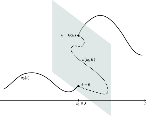
Figure 4. A two-speed solution.

6. Conclusion

The present manuscript aims to make a contribution to the mathematical modelling of large-strain elasto-plasticity and to provide a conceptual framework for existence theorems. Future work will cast the concepts introduced into this work, in particular the two-speed solutions, into a mathematically rigorous framework and perform a thorough mathematical analysis.

Acknowledgements

I would like to thank Sergio Conti, Georg Dolzmann, Gilles Francfort, Michael Ortiz, Ulisse Stefanelli, Florian Theil, and Emil Wiedemann (in particular, Example 3.3 is due to him) for many interesting discussions related to the present work. The support of the author through the EPSRC Research Fellowship EP/L018934/1 on “Singularities in Nonlinear PDEs” and through the Royal Society Travel Grant IE131532 is gratefully acknowledged.

Author’s biography

Filip Rindler has held the post of Zeeman Lecturer (Assistant Professor) in Mathematics at the University of Warwick since 2013. After completing his doctorate in nonlinear PDE theory and the calculus of variations at the OxPDE centre within the University of Oxford in 2011, he moved to the University of Cambridge to take up the Gonville & Caius College Drosier Research Fellowship, holding the position until 2015 (on leave 2013–2015). For 2014–2017 he is funded by a full-time EPSRC Research Fellowship on “Singularities in Nonlinear PDEs”.

References

• [1] R. Abbaschian, L. Abbaschian, and R. E. Reed-Hill, Physical Metallurgy Principles - SI Edition, Cengage Learning, 2009.
• [2] L. Ambrosio, N. Fusco, and D. Pallara, Functions of Bounded Variation and Free-Discontinuity Problems, Oxford Mathematical Monographs, Oxford University Press, 2000.
• [3] R. W. Armstrong, W. Arnold, and F. J. Zerilli, Dislocation mechanics of copper and iron in high rate deformation tests, J. Appl. Phys. 105 (2009), 023511.
• [4] E. Ben-David, T. Tepper-Faran, D. Rittel, and D. Shilo, A large strain rate effect in thin free-standing Al films, Scripta Materialia 90–91 (2014), 6–9.
• [5] J. Casey and P. M. Naghdi, A Remark on the Use of the Decomposition F = FeFp in Plasticity, J. Appl. Mech. 47 (1980), 672–675.
• [6] P. Ciarlet, Mathematical Elasticity, vol. 1: Three Dimensional Elasticity, North-Holland, 1988.
• [7] B. D. Coleman and W. Noll, The thermodynamics of elastic materials with heat conduction and viscosity, Arch. Ration. Mech. Anal. 13 (1963), no. 1, 167–178.
• [8] S. Conti and F. Theil, Single-Slip Elastoplastic Microstructures, Arch. Ration. Mech. Anal. 178 (2005), 125–148.
• [9] Y. F. Dafalias, Issues on the constitutive formulation at large elastoplastic deformations, part 1: Kinematics, Acta Mech. 69 (1987), 119–138.
• [10] G. Dal Maso, A. DeSimone, and F. Solombrino, Quasistatic evolution for Cam-Clay plasticity: a weak formulation via viscoplastic regularization and time rescaling, Calc. Var. Partial Differential Equations 40 (2010), 125–181.
• [11] by same author, Quasistatic evolution for Cam-Clay plasticity: properties of the viscosity solution, Calculus of Variations and Partial Differential Equations 44 (2011), 495–541.
• [12] T. M. De Hossony, A. Roos, and E. D. Metselaar, Temperature rise due to fast-moving dislocations, Philos. Mag. A 81 (2001), 1099–1120.
• [13] L. C. Evans and R. F. Gariepy, Measure Theory and Fine Properties of Functions, Studies in Advanced Mathematics, CRC Press, 1992.
• [14] G. A. Francfort and A. Mielke, Existence results for a class of rate-independent material models with nonconvex elastic energies, J. Reine Angew. Math. 595 (2006), 55–91.
• [15] M. Frémond, Non-Smooth Thermomechanics, Springer, 2002.
• [16] D. Grandi and U. Stefanelli, Finite plasticity in PT P, arXiv:1509.08681, 2015.
• [17] A. E. Green and P. M. Naghdi, Some remarks on elastic-plastic deformation at finite strain, International Journal of Engineering Science 9 (1971), 1219–1229.
• [18] M. E. Gurtin, On the plasticity of single crystals: free energy, microforces, plastic-strain gradients, J. Mech. Phys. Solids 48 (2000), 989–1036.
• [19] M. E. Gurtin, E. Fried, and L. Anand, The mechanics and thermodynamics of continua, Cambridge University Press, 2010. MR 2884384 (2012m:74001)
• [20] B. C. Hall, Lie groups, Lie algebras, and representations, Graduate Texts in Mathematics, vol. 222, Springer, 2003.
• [21] W. Han and B. D. Reddy, Plasticity – Mathematical Theory and Numerical Analysis, Interdisciplinary Applied Mathematics, vol. 9, Springer, 2013.
• [22] T. Hochrainer, S. Sandfeld, M. Zaiser, and P. Gumbsch, Continuum dislocation dynamics: Towards a physical theory of crystal plasticity, Journal of the Mechanics and Physics of Solids 63 (2014), 167–178.
• [23] T Hochrainer, M Zaiser, and P Gumbsch, A three-dimensional continuum theory of dislocation systems: kinematics and mean-field formulation, Philos. Mag. 87 (2007), 1261–1282.
• [24] M. E. Kassner, P. Geantil, L. E. Levine, and B. C. Larson, Backstress, the Bauschinger effect and cyclic deformation, Mater. Sci. Forum 604–605 (2009), 39–51.
• [25] E. Kröner, Allgemeine Kontinuumstheorie der Versetzungen und Eigenspannungen, Arch. Ration. Mech. Anal. (1960), 273–334.
• [26] by same author, Benefits and shortcomings of the continuous theory of dislocations, Int. J. Solids Struct. 38 (2001), 1115–1134.
• [27] E. H. Lee, Elastic-plastic deformation at finite strain, ASME J. Appl. Mech. 36 (1969), 1–6.
• [28] E. H. Lee and D. T. Liu, Finite-strain elastic-plastic theory with application to plane-wave analysis, J. Appl. Phys. 38 (1967), 19–27.
• [29] J. M. Lee, Introduction to Smooth Manifolds, 2nd ed., Graduate Texts in Mathematics, vol. 218, Springer, 2013.
• [30] J. Lemaitre and J.-L. Chaboche, Mechanics of solid materials, Cambridge University Press, 1990.
• [31] V. A. Lubarda and E. H. Lee, A Correct Definition of Elastic and Plastic Deformation and Its Computational Significance, J. Appl. Mech. 48 (1981), 35, Erratum: J. Appl. Mech. 48 (1981), 686.
• [32] J. Lubliner, Plasticity Theory, Dover, 2008.
• [33] A. Mainik and A. Mielke, Existence results for energetic models for rate-independent systems, Calc. Var. Partial Differential Equations 22 (2005), 73–99.
• [34] A. Mainik and A. Mielke, Global existence for rate-independent gradient plasticity at finite strain, J. Nonlinear Sci. 19 (2009), 221–248.
• [35] J. Mandel, Equations constitutives et directeurs dans les milieux plastiques et viscoplastiques, Int. J. Solids Struct. 9 (1973), 725–740.
• [36] A. Mielke, Finite elastoplasticity Lie groups and geodesics on ${\rm SL}(d)$, Geometry, mechanics, and dynamics, Springer, 2002, pp. 61–90.
• [37] by same author, Energetic formulation of multiplicative elasto-plasticity using dissipation distances, Contin. Mech. Thermodyn. 15 (2003), 351–382.
• [38] A. Mielke and S. Müller, Lower semicontinuity and existence of minimizers in incremental finite-strain elastoplasticity, ZAMM Z. Angew. Math. Mech. 86 (2006), 233–250.
• [39] A. Mielke and F. Rindler, Reverse approximation of energetic solutions to rate-independent processes, NoDEA Nonlinear Differential Equations Appl. 16 (2009), 17–40.
• [40] A. Mielke, R. Rossi, and G. Savaré, Modeling solutions with jumps for rate-independent systems on metric spaces, Discrete Contin. Dyn. Syst. 25 (2009), 585–615.
• [41] by same author, BV solutions and viscosity approximations of rate-independent systems, ESAIM Control Optim. Calc. Var. 18 (2012), 36–80.
• [42] A. Mielke and T. Roubíček, Rate-Independent Systems: Theory and Application., Applied Mathematical Sciences, vol. 193, Springer, 2015.
• [43] A. Mielke and F. Theil, A mathematical model for rate-independent phase transformations with hysteresis, Proceedings of the Workshop on “Models of Continuum Mechanics in Analysis and Engineering” (H.-D. Alber, R.M. Balean, and R. Farwig, eds.), Shaker Verlag, 1999, pp. 117–129.
• [44] by same author, On rate-independent hysteresis models, NoDEA Nonlinear Differential Equations Appl. 11 (2004), 151–189.
• [45] A. Mielke, F. Theil, and V. I. Levitas, A variational formulation of rate-independent phase transformations using an extremum principle, Arch. Ration. Mech. Anal. 162 (2002), 137–177.
• [46] P. M. Naghdi, A critical review of the state of finite plasticity, ZAMP Zeitschrift für angewandte Mathematik und Physik 41 (1990), 315–394.
• [47] S. Nemat-Nasser, Decomposition of strain measures and their rates in finite deformation elastoplasticity, Int. J. Solids Struct. 15 (1979), 155–166.
• [48] M. Ortiz and E. A. Repetto, Nonconvex energy minimization and dislocation structures in ductile single crystals, J. Mech. Phys. Solids 47 (1999), 397–462.
• [49] C. Reina and S. Conti, Kinematic description of crystal plasticity in the finite kinematic framework: A micromechanical understanding of F=FeFp, J. Mech. Phys. Solids 67 (2014), 40–61.
• [50] J. R. Rice, Inelastic constitutive relations for solids: An internal-variable theory and its application to metal plasticity, J. Mech. Phys. Solids 19 (1971), 433–455.
• [51] F. Rindler, Two-speed solutions for rate-independent systems, forthcoming, 2015.
• [52] R. T. Rockafellar, Convex Analysis, Princeton Mathematical Series, vol. 28, Princeton University Press, 1970.
• [53] S. Sandfeld, T. Hochrainer, M. Zaiser, and P. Gumbsch, Continuum modeling of dislocation plasticity: Theory, numerical implementation, and validation by discrete dislocation simulations, J. Mater. Res. 26 (2011), 623–632.
• [54] M. Silhavy, The Mechanics and Thermodynamics of Continuous Media, Springer, 1997.
• [55] U. Stefanelli, A Variational Principle for Hardening Elastoplasticity, SIAM J. Math. Anal. 40 (2008), 623–652.
• [56] by same author, A variational characterization of rate-independent evolution, Math. Nachr. 282 (2009), 1492–1512.
• [57] H. M. Zbib, On the mechanics of large inelastic deformations: kinematics and constitutive modeling, Acta Mechanica 96 (1993), 119–138.
• [58] H. Ziegler and C. Wehrli, The derivation of constitutive relations from the free energy and the dissipation function, Advances in applied mechanics, Vol. 25, Adv. Appl. Mech., vol. 25, Academic Press, 1987, pp. 183–237.