Unraveling coherent quantum feedback for Pyragas control

Abstract

We present a Heisenberg operator based formulation of coherent quantum feedback and Pyragas control. This model is easy to implement and allows for an efficient and fast calculation of the dynamics of feedback-driven observables as the number of contributing correlations grows in systems with a fixed number of excitations only linearly in time. Furthermore, our model unravels the quantum kinetics of entanglement growth in the system by explicitly calculating non-Markovian multi-time correlations, e.g., how the emission of a photon is correlated with an absorption process in the past. Therefore, the time-delayed differential equations are expressed in terms of insightful physical quantities. Another considerate advantage of this method is its compatibility to typical approximation schemes, such as factorization techniques and the semi-classical treatment of coherent fields. This allows the application on a variety of setups, ranging from closed quantum systems in the few excitation regimes to open systems and Pyragas control in general.

March 16, 2024

Figure 1: We investigate an intrinsic and coherent feedback mechanism, where a system is driven by its own past via a continuum of modes. The roundtrip time $\tau=2L/c$ scales with the length between the system and the mirror. The feedback strength is determined by the coupling constant $g$.

I Introduction

Controlling quantum systems with respect to their coherence properties, quantum states and dynamics is a basic requirement for quantum information science applications zoller-roadmap ; Wiseman::09 ; brandes2015feedback . The possibilities range from coherent control of quantum systems involving higher order coherence processes kiraz2004quantum ; wolters2014deterministic to open loop feedback control schemes Wiseman::09 ; sayrin2011real . Alternatively, structured continua allow state preserving measurement-free coherent control schemes for time-delayed self-feedback, i.e. the subsequent interaction of the system with former states of itself dorner-half-cavities ; carmele2013single ; grimsmo2015time ; pichler2015photonic . Such a feedback mechanism combines the advantage of time delayed feedback control with coherent quantum control in order to manipulate distinctive system degrees of freedom.

Quantum self-feedback mechanisms are often based on a structured continuum with multi-mode environmental degrees of freedom cook1987quantum ; alber1992photon ; tufarelli2014non ; hein2014optical ; hughes2007coupled . In this paper, we develop a Heisenberg-operator technique for a convenient implementation of coherent feedback via the interaction of a quantum system with a quasi-continuous bosonic reservoir hetet2011single ; albert2011observing ; hughes2007coupled , related to the Langevin approach gardiner-book .

In the following, the reservoir degrees of freedom are eliminated in favor of system operators inheriting the feedback delay time. The complexity of the multi-mode reservoir is transfered to the handling of multi-time-correlations. This approach allows a straight forward treatment of coherent time delayed quantum feedback, with a drastic reduction of numerical effort. Furthermore, it gives access to the feedback mechanism as the entanglement growth is expressed in physical meaningful quantities, e.g. the creation and annihilation of a photon at two different times. These time-correlated quantities provide insight and allow the application of factorization techniques, as the degree of entanglement is directly accessible. Factorization such as cluster expansion kira2011semiconductor and Born approximation are unavoidable if the transient feeback regime albert2011observing ; schulze2014feedback between classical lang1980external ; kantner2015delay ; wegert2014integrated ; flunkert2013dynamics and quantum feedback is under investigation hetet2011single ; glaetzle2010single .

The paper is organized as following. After this introduction, Sec. I, and before introducing feedback Heisenberg operators, we provide a short review of existing exact models, which form the backbone of future developments and also include the basic ingredients of coherent feedback control, Sec. II. In Sec. III, we derive the basic equation of motion for the Heisenberg operators and provide an analytical solution in case of an empty cavity coupling to a structured continuum lei2012quantum . Given the operator dynamics, we derive the model to stabilize Rabi oscillations inside a cavity and unravel the otherwise hidden feedback mechanism, before we conclude in Sec. IV.

II Analytical solutions in the Schrödinger Picture

In this section, we give three examples for analytically solvable coherent quantum self-feedback models. These models are an important benchmark for numerical implementations and contain the basic features of quantum feedback. All three examples restrict the system dynamics to the single-excitation regime and thus describe a linear quantum feedback mechanism.

Following the experimental realization of a decaying single-atom in front of a mirror hetet2011single , an analytical model for this scenario has been provided dorner-half-cavities ; cook1987quantum ; glaetzle2010single ; kabuss2015analytical . The Hamiltonian includes the radiative coupling of the atomic two-level system to the photon continuum with a boundary condition, imposing the feedback mechanism $(\hbar=1)$:

$$H =\omega_{e}P^{\dagger}P+\int\text{d}k\ \left(\omega_{k}\ d^{\dagger}_{k}d^{\phantom{\dagger}}_{k}+g_{k}P^{\dagger}d^{\phantom{\dagger}}_{k}+g^{*}_{k}d^{\dagger}_{k}P\right),$$ (1)

where $P=\left|g\right\rangle\left\langle e\right|$ denotes the atomic operators for the excited- $\left|e\right\rangle$ and ground-state $\left|g\right\rangle$. The radiative continuum is included via the photonic creation and annihilation operators $d^{(\dagger)}_{k}$ for a photon in the mode $k=\omega/c$ ($c$: the vacuum speed of light). The coupling between the atom and the radiative continuum is denoted by $g(k)=g_{0}\sin(kL)$ and includes the mirror imposed boundary condition at a distance between mirror and atom of $L$ with a strength of $g_{0}$. The length defines the feedback roundtrip time with $\tau=2L/c$.

Assuming for the radiative continuum the vacuum state $b^{\phantom{\dagger}}_{k}\left|\Psi(0)\right\rangle=0$, the Hilbert space is restricted to a single excitation either in the atomic or photonic degrees of freedom. The wave vector of the system reads:

$$\left|\Psi(t)\right\rangle= c_{e}(t)\left|e,\{0\}_{k}\right\rangle+\int\text{d}k\ c^{k}_{g}(t)\left|g,\{1\}_{k}\right\rangle,$$ (2)

with the excitation in the atom or in the photonic continuum, respectively. After applying the Schrödinger equation and formally integrating the equation for $\dot{c}^{k}_{g}$, the equation for the coefficient for the excited state $c_{e}$ reads:

$$\dot{c_{e}}(t)= -\Gamma c_{e}(t)+\Gamma_{\tau}c_{e}(t-\tau)\Theta(t-\tau),$$ (3)

with $\Gamma=\pi g_{0}^{2}/c$, $\Gamma_{\tau}=\Gamma\exp[i\omega_{e}\tau]$, and $\Theta(x)$ the Heaviside function: $\Theta(x)=0$ for $x\leq 0$ and $\Theta(x)=1$ for $x>0$. Here, the basic ingredient of Pyragas control $K\left[f(t)-f(t-\tau)\right]$ are given as $K$ allows the control of periodic orbits such as Rabi oscillations or relaxation ocillations flunkert2011time . This differential equation of motion can be solved in the Laplace domain, yielding the following dynamics:

$$c_{e}(t)= \sum_{n=0}^{\infty}\frac{e^{-\Gamma t}}{n!}\left(\Gamma_{\tau}e^{\Gamma_{\tau}\tau}(t-n\tau)\right)^{n}\Theta(t-n\tau).$$ (4)

The same solution is obtained, if instead of an atom a bosonic mode decays such as a cavity photon with the following Hamiltonian:

$$H =\omega_{0}c^{\dagger}c+\int\text{d}k\ \left(\omega_{k}\ d^{\dagger}_{k}d^{\phantom{\dagger}}_{k}+g_{k}c^{\dagger}d^{\phantom{\dagger}}_{k}+g^{*}_{k}d^{\dagger}_{k}c\right),$$ (5)

with $c^{(\dagger)}$ creating (annhiliating) a cavity photon with frequency $\omega_{0}$ and $[c,c^{\dagger}]=1$. Replacing in the derivation above $e\rightarrow 1$ and $g\rightarrow 0$, the same solution applies to this situation as well. This is a consequence of the single-excitation limit, where the qubit and the bosonic mode cannot be distinguish from each other and quantum non-linearities are yet not included.

It is possible to derive an analytical solution even for a combined model, where an emitter is coupled to a cavity mode and the cavity mode decays into the radiative continuum. The Hamiltonian reads:

$$H =\omega_{e}P^{\dagger}P+\omega_{0}c^{\dagger}c+\int\text{d}k\ \omega_{k}\ d^{\dagger}_{k}d^{\phantom{\dagger}}_{k}$$

$$+M\left(P^{\dagger}c+c^{\dagger}P\right)+\int\text{d}k\ \left(g_{k}c^{\dagger}d^{\phantom{\dagger}}_{k}+g^{*}_{k}d^{\dagger}_{k}c\right),$$ (6)

where the cavity-emitter coupling strength is denoted by $M$ and the full wave vector includes now three states: The wave vector of the system reads:

$$\left|\Psi(t)\right\rangle= c_{e}(t)\left|e,0,\{0\}_{k}\right\rangle+c_{g}(t)\left|g,1,\{0\}_{k}\right\rangle+\int\text{d}k\ c^{k}_{g}(t)\left|g,0,\{1\}_{k}\right\rangle,$$ (7)

with the excitation in the emitter, cavity or in the photonic continuum, respectively. The differential equation for the ground state with one photon in the cavity reads:

$$\dot{c_{g}}= -\Gamma c_{g}-iMc_{e}+\Gamma_{\tau}c_{g}(t-\tau)\Theta(t-\tau).$$ (8)

Applying the binomial series and the Laplace transformation: $n!/(s-a)^{n+1}\rightarrow t^{n}\exp[at]$, we yield an expression in the time domain, after choosing $M=\Gamma/2$ to simplify the expression:

$$c_{g}(t) =\frac{i}{2}\sum_{n=0}^{\infty}n!2^{n+1}e^{-\Gamma/2(t-n\tau)+i\omega_{0}n\tau}\Theta(t-n\tau)$$

$$\sum_{k=0}^{n}\frac{(-1)^{k}}{k!(n-k)!}\frac{\left[(t-n\tau)\Gamma/2\right]^{n+1+k}}{(n+1+k)!}.$$ (9)

These analytical solutions are given to benchmark the numerical implementations. They contain already interesting features such as modified decaying rates dorner-half-cavities ; eschner2001light , Rabi oscillations stabilization carmele2013single ; grimsmo2015time , entangling cavities within a quantum eraser set-up hein2015entanglement or enhanced photon polarization entanglement stemming from a controlled biexciton cascade hein2014optical . The delay phase and the delay strength provide an interesting new degree of freedom to manipulate quantum systems in a self-sustained, closed-loop and non-invasive approach. To unravel coherent quantum feedback and link the feedback mechanism directly to observable quantities, we switch now to the Heisenberg picture and express the dynamics in terms of time-dependent operators instead of wave vector coefficients.

III Quantum Feeback in the Heisenberg picture

We investigate the case of boson-boson coupling to include the feedback mechanism. We present a way to include coherent quantum self-feedback consistently at a operator level, i.e. with the Langevin operator technique gardiner-book ; carmele2014opto . We derive the necessary equations of motion and benchmark our method with the analytical solutions from the previous section. Hereby, we gain insight into the mechanism that leads e.g. to the stabilization of the Rabi oscillations.

III.1 Equation of motion - approach

We start with the Hamiltonian (6), where the emitter is coupled to a cavity mode and the cavity mode couples to the radiative continuum, leading to a decay of the cavity mode as well as to feedback. First, we solve the bilinear Hamiltonian in the Heisenberg equation of motion approach $-i\dot{A}=[H,A]$ with $A$ being an arbitrary, non-explicitly time dependent operator $(\hbar=1)$. The equation of motion (EOM) for the reservoir operator $d^{\phantom{\dagger}}_{k}$ is derived via the Heisenberg equation of motion:

$$\dot{d^{\phantom{\dagger}}_{k}}=-i\omega_{k}d^{\phantom{\dagger}}_{k}-ig^{*}_{k}\ c.$$ (10)

Formally integrating yields:

$$d^{\phantom{\dagger}}_{k}(t)=d_{k}(0)\ e^{-i\omega_{k}t}-i\int_{0}^{t}\text{d}t\ ^{\prime}g^{*}_{k}e^{-i\omega_{k}(t-t^{\prime})}\ c(t^{\prime}).$$ (11)

So, we can include the reservoir interaction by plugging this solution into the equation of motion of the system boson operator:

$$\dot{c} =-i\omega_{c}\ c-iM\ P-i\int\ \text{d}k\ \ g_{k}\ d_{k}(t^{\prime})$$ (12)

$$=-i\omega_{c}\ c-iM\ P-i\int\text{d}k\ \ d_{k}(0)e^{-i\omega_{k}t}g_{k}-\int_{0}^{t}\text{d}t\ ^{\prime}\ c(t^{\prime})f(t,t^{\prime}).$$

The function $f(t,t^{\prime})$ includes the structure of the reservoir and can be evaluated as the operator is independent of the wave number $k$:

$$f(t,t^{\prime}):=\int\text{d}k\ |g_{k}|^{2}e^{-i\omega_{k}(t-t^{\prime})}.$$ (13)

If $g_{k}\equiv g_{0}$, the function yields $f(t,t^{\prime})=2\pi\delta(t-t^{\prime})g_{0}^{2}/c=2\Gamma\delta(t-t^{\prime})$ with the definition for the loss coefficient. If $g_{k}=g_{0}\sin(kL)$, we have a structured continuum with a feedback mechanism and the function reads with $\tau=2L/c$:

$$f(t,t^{\prime})=\Gamma\left(2\delta(t-t^{\prime})-\delta(t-t^{\prime}-\tau)-\delta(t-t^{\prime}+\tau)\right).$$ (14)

The equation of motion of the bosonic system operator with feedback reads, having in mind that $t^{\prime}\leq t$:

$$\dot{c} =-\left(i\omega_{c}+\Gamma\right)\ c(t)-iM\ P+\Gamma_{\tau}c(t-\tau)\Theta(t-\tau)-i\Delta B(t),$$ (15)

with the noise operator $\Delta B(t)=\int\text{d}k\ \ d_{k}(0)e^{-i\omega_{k}t}g_{k}$.

III.2 Photon-Photon coupling

Setting the cavity-emitter coupling to zero ($M=0$), the excitation manifolds of the photon-operator decouple and the problem can be solved analytically. The solution of the photon operator in (15), subjected to feedback, but not coupled to an emitter reads:

$$c(t)= e^{-\Gamma t}\left(c(0)+\Gamma_{\tau}\int_{0}^{t}\text{d}t\ ^{\prime}e^{\Gamma t^{\prime}}\Theta(t^{\prime}-\tau)c(t^{\prime}-\tau)\right),$$ (16)

where the noise term $\Delta B(t)$ is omitted. This can be justified by assuming a structured continuum initially in the vacuum state and by keeping throughout the calculation the normal-ordering. Given this general calculation, we need the initial state of the cavity system, e.g. ${\langle}c^{\dagger}(0)c(0){\rangle}=N$. For the first time interval ($t_{0}\in[0,\tau]$), one yields

$${\langle}c^{\dagger}(t_{0})c(t_{0}){\rangle}= {\langle}e^{-\Gamma t_{0}}c^{\dagger}(0)e^{-\Gamma t_{0}}c(0){\rangle}=Ne^{-2\Gamma t_{0}},$$ (17)

The integral part of the solution does not contribute as $t<\tau$. The two-time correlation in the first time interval reads: ${\langle}c^{\dagger}(t_{0})c(0){\rangle}=Ne^{-\Gamma t_{0}}$. For the second time interval ($t_{1}\in[\tau,2\tau]$) one yields,

$${\langle}c^{\dagger}(t_{1})c(t_{1}){\rangle} =Ne^{-2\Gamma t_{1}}$$ (18)

$$+e^{-2\Gamma t_{1}}\text{Re}\left[\Gamma_{\tau}\int_{\tau}^{t_{1}}\text{d}t\ ^{\prime}e^{\Gamma t^{\prime}}{\langle}c^{\dagger}(t^{\prime}-\tau)c(0){\rangle}\right]$$

$$+|\Gamma_{\tau}|^{2}\int_{\tau}^{t_{1}}\text{d}t\ ^{\prime}e^{\Gamma t^{\prime}-2\Gamma t_{1}}\int_{\tau}^{t_{1}}\text{d}t\ ^{\prime\prime}e^{\Gamma t^{\prime\prime}}{\langle}c^{\dagger}(t^{\prime}-\tau)c(t^{\prime\prime}-\tau){\rangle},$$

now we can use the solution from the time interval before, as ${\langle}c^{\dagger}(t^{\prime}-\tau)c(t^{\prime\prime}-\tau){\rangle}=N\exp[-\Gamma(t^{\prime}-\tau+t^{\prime\prime}-\tau)]$. We derive, after formally integrating:

$${\langle}c^{\dagger}(t_{1})c(t_{1}){\rangle} =N|\Gamma_{\tau}|^{2}e^{-2\Gamma(t_{1}-\tau)}(t_{1}-\tau)^{2}$$ (19)

$$+N2\text{Re}\left[\Gamma_{\tau}\right]e^{-\Gamma(2t_{1}-\tau)}(t_{1}-\tau)+Ne^{-\Gamma 2t_{1}}.$$

This procedure allows by means of simple integration to calculate all higher moments of the photon-correlations. However, due to the linear coupling, the photon statistics is not changed and feedback does not provide more than a excitation exchange between the cavity and the continuum. In the next section, we calculate a more complex problem and demonstrate, that feedback can lead to a stabilization of Rabi oscillations between an emitter and the cavity mode.

III.3 Hierarchy problem and scaling properties

To illustrate the method, we reproduce within the Heisenberg picture the solution given in (9). For this scenario, initially an emitter decays into the cavity mode and this cavity mode is damped and then driven by the self-feedback after a roundtrip time $\tau$. The relevant equations of motion are derived for $n$ feedback intervals and are discussed with respect to the new occurring quantities. It will become clear, that the coupling of a single bosonic mode to the feedback reservoir constitutes in the single excitation limit a very specific scenario, where most complications arising from the time-ordering procedure can be omitted. The basic set of equations of motion, involving the photon coherence $c$ and the electronic polarization $P$, that are used to derive the time-correlated dynamics of the system are given by:

$$\dot{c}_{j} = -\Gamma c_{j}+\Gamma_{\tau}c_{j+1}\Theta_{j+1}-iM\ P_{j},$$ (20)

$$\dot{P}_{j} = 2iM\ P_{j}^{\dagger}P_{j}c_{j}-iM\ c_{j},$$ (21)

where $c_{j}\equiv c(t-j\tau)$ and $t_{j}\equiv t-j\tau$ and the noise term is omitted again. The noise term can be omitted, as long the normal-ordering is conserved and initially a vacuum state for the reservoir is assumed. The single excitation limit is specific as the normal-ordering is preserved for all times automatically.

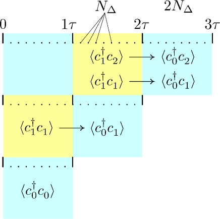
Figure 2: Illustration of memory growth: For calculating the dynamics in $\tau$-interval $i\mathrel{\hat{=}}[i\tau,(i+1)\tau)$ it is necessary to store $3iN_{\Delta}$ two-time correlations. Only information from the previous time interval $i-1$ is needed. $N_{\Delta}$ is the number of time discretization steps.

The electronic degree of freedom $P$ couples only to the cavity mode via the electron-photon coupling strength, while the cavity coherence $c$ according to (6) is also subject to the photon feedback. (20) and (21) are valid for any time interval $t_{0}\in[i\tau,(i+1)\tau)$ with the advantage, that expectation values of previous times, such as $\langle A_{n}B_{m}\rangle$ have already been calculated on the fly. Starting with the $t=0$, the equations of motion correspond to the case of a dissipative Jaynes-Cummings model (JCM): $t_{0}\equiv t\in[0,\tau)$

$$\partial_{t}{\langle}c^{\dagger}_{0}c^{\phantom{\dagger}}_{0}{\rangle} = -2\Gamma{\langle}c^{\dagger}_{0}c^{\phantom{\dagger}}_{0}{\rangle}+2\text{Im}\bigl{[}M\ {\langle}P^{\dagger}_{0}c^{\phantom{\dagger}}_{0}{\rangle}\bigr{]},$$ (22)

$$\partial_{t}{\langle}P^{\dagger}_{0}c^{\phantom{\dagger}}_{0}{\rangle} = -\Gamma{\langle}P^{\dagger}_{0}c^{\phantom{\dagger}}_{0}{\rangle}+iM\ {\langle}c^{\dagger}_{0}c^{\phantom{\dagger}}_{0}{\rangle}-iM\ {\langle}P^{\dagger}_{0}P^{\phantom{\dagger}}_{0}{\rangle},$$ (23)

$$\partial_{t}{\langle}P^{\dagger}_{0}P^{\phantom{\dagger}}_{0}{\rangle} = -2\text{Im}\bigl{[}M\ {\langle}P^{\dagger}_{0}c^{\phantom{\dagger}}_{0}{\rangle}\bigr{]}.$$ (24)

In the second $\tau$-interval, the EOMs contain additional terms in the form of two-time correlated expectation values: $t_{0}\in[\tau,2\tau)$ and $t_{1}\in[0,\tau)$:

$$\partial_{t}{\langle}c^{\dagger}_{0}c^{\phantom{\dagger}}_{0}{\rangle} = -2\Gamma{\langle}c^{\dagger}_{0}c^{\phantom{\dagger}}_{0}{\rangle}+2\text{Re}\bigl{[}{\langle}\Gamma_{\tau}c^{\dagger}_{0}c_{1}^{\phantom{\dagger}}{\rangle}\bigr{]}$$

$$+ 2\text{Im}\bigl{[}M\ {\langle}P^{\dagger}_{0}c^{\phantom{\dagger}}_{0}{\rangle}\bigr{]},$$

$$\partial_{t}{\langle}P^{\dagger}_{0}P^{\phantom{\dagger}}_{0}{\rangle} = -2\text{Im}\bigl{[}M\ {\langle}P^{\dagger}_{0}c^{\phantom{\dagger}}_{0}{\rangle}\bigr{]}$$ (26)

$$\partial_{t}{\langle}P^{\dagger}_{0}c^{\phantom{\dagger}}_{0}{\rangle} = -\Gamma{\langle}P^{\dagger}_{0}c^{\phantom{\dagger}}_{0}{\rangle}+\Gamma_{\tau}{\langle}P^{\dagger}_{0}c^{\phantom{\dagger}}_{1}{\rangle}$$

$$+ iM\ {\langle}c^{\dagger}_{0}c^{\phantom{\dagger}}_{0}{\rangle}-iM\ {\langle}P^{\dagger}_{0}P^{\phantom{\dagger}}_{0}{\rangle},$$

$$\partial_{t}{\langle}c^{\dagger}_{0}c^{\phantom{\dagger}}_{1}{\rangle} = -2\Gamma{\langle}c^{\dagger}_{0}c^{\phantom{\dagger}}_{1}{\rangle}+\Gamma_{\tau}^{*}{\langle}c^{\dagger}_{1}c^{\phantom{\dagger}}_{1}{\rangle}$$

$$+ iM\ {\langle}P^{\dagger}_{0}c_{1}{\rangle}-iM\ {\langle}c^{\dagger}_{0}P^{\phantom{\dagger}}_{1}{\rangle},$$

$$\partial_{t}{\langle}P^{\dagger}_{0}c^{\phantom{\dagger}}_{1}{\rangle} = -\Gamma{\langle}P^{\dagger}_{0}c^{\phantom{\dagger}}_{1}{\rangle}+iM\ {\langle}c^{\dagger}_{0}c^{\phantom{\dagger}}_{1}{\rangle}-iM{\langle}P^{\dagger}_{0}P^{\phantom{\dagger}}_{1}{\rangle},$$ (29)

$$\partial{\langle}c^{\dagger}_{0}P^{\phantom{\dagger}}_{1}{\rangle} = -\Gamma{\langle}c^{\dagger}_{0}P^{\phantom{\dagger}}_{1}{\rangle}+\Gamma_{\tau}^{*}{\langle}c_{1}^{\dagger}P^{\phantom{\dagger}}_{1}{\rangle}$$

$$- iM{\langle}c^{\dagger}_{0}c^{\phantom{\dagger}}_{1}{\rangle}+iM{\langle}P^{\dagger}_{0}P^{\phantom{\dagger}}_{1}{\rangle},$$

$$\partial_{t}{\langle}P^{\dagger}_{0}P^{\phantom{\dagger}}_{1}{\rangle} = iM\ {\langle}c^{\dagger}_{0}P^{\phantom{\dagger}}_{1}{\rangle}-iM\ {\langle}P^{\dagger}_{0}c^{\phantom{\dagger}}_{1}{\rangle}$$ (31)

For this second time interval, there are no additional EOMs required, since correlations such as ${\langle}c^{\dagger}_{i}c^{\phantom{\dagger}}_{j}{\rangle}$, ${\langle}P^{\dagger}_{i}c^{\phantom{\dagger}}_{j}{\rangle}$ and ${\langle}P^{\dagger}_{i}P^{\phantom{\dagger}}_{j}{\rangle}$, with $i,j>0$, are already included within (22)-(24) of the previous time interval. With this, in an arbitrary $\tau$-interval the EOMs thus result in: $t_{0}\in[i\tau,(i+1)\tau)$

$$\partial_{t}{\langle}c^{\dagger}_{0}c^{\phantom{\dagger}}_{j}{\rangle} = -2\Gamma{\langle}c^{\dagger}_{0}c^{\phantom{\dagger}}_{j}{\rangle}+\Gamma_{\tau}^{*}{\langle}c^{\dagger}_{0}c^{\phantom{\dagger}}_{j}{\rangle}+\Gamma_{\tau}{\langle}c^{\dagger}_{0}c^{\phantom{\dagger}}_{j+1}{\rangle}\Theta_{j+1}$$ (32)

$$+ ig{\langle}P^{\dagger}_{0}c_{j}{\rangle}-iM\ {\langle}c^{\dagger}_{0}P^{\phantom{\dagger}}_{j}{\rangle},$$

$$\partial_{t}{\langle}P^{\dagger}_{0}c^{\phantom{\dagger}}_{j}{\rangle} = -\Gamma{\langle}P^{\dagger}_{0}c^{\phantom{\dagger}}_{j}{\rangle}+\Gamma_{\tau}{\langle}P^{\dagger}_{0}c^{\phantom{\dagger}}_{j+1}{\rangle}\Theta_{j+1}$$

$$+ iM\ {\langle}c^{\dagger}_{0}c^{\phantom{\dagger}}_{j}{\rangle}-iM{\langle}P^{\dagger}_{0}P^{\phantom{\dagger}}_{j}{\rangle},$$

$$\partial{\langle}c^{\dagger}_{0}P^{\phantom{\dagger}}_{j}{\rangle} = -\Gamma{\langle}c^{\dagger}_{0}P^{\phantom{\dagger}}_{j}{\rangle}+\Gamma_{\tau}^{*}{\langle}c_{1}^{\dagger}P^{\phantom{\dagger}}_{j}{\rangle}$$

$$- iM\ {\langle}c^{\dagger}_{0}c^{\phantom{\dagger}}_{j}{\rangle}+iM\ {\langle}P^{\dagger}_{0}P^{\phantom{\dagger}}_{j}{\rangle},$$

$$\partial_{t}{\langle}P^{\dagger}_{0}P^{\phantom{\dagger}}_{j}{\rangle} = iM\ {\langle}c^{\dagger}_{0}P^{\phantom{\dagger}}_{j}{\rangle}-iM\ {\langle}P^{\dagger}_{0}c^{\phantom{\dagger}}_{j}{\rangle}$$ (35)

Here $j$ can be any number from $0$ and $i$. At first sight it seems necessary to memorize any possible two-time correlation ${\langle}A_{n}B_{m}{\rangle}$ in order to compute this growing set of equations. However this is not the case. Instead, the number of quantities to memorize grows linearly with the index $i$ of the time-interval [See Fig. 2]. Solving the Block of (32) - (35) of the $i$-th interval, for any time delay $j\tau\leq i\tau$, only two quantities at each $j$ from previous times have to be stored:

$$\text{For}\quad j\leq i\quad\longrightarrow\quad\{{\langle}c^{\dagger}_{1}c^{\phantom{\dagger}}_{j}{\rangle},\ {\langle}c^{\dagger}_{1}P^{\phantom{\dagger}}_{j}{\rangle}\}^{\phantom{\dagger}}_{j},$$ (36)

the number of quantities to be stored scales linearly with the number of time discretization steps $N_{\Delta}$ as illustrated in Fig. 2. Most of the previous two-time-correlations do not couple into the set of equations of the $i$th interval, so that the numerical effort as well as the memory cost is drastically reduced. Next to the dynamic memory incorporated within quantities such as ${\langle}c^{\dagger}_{1}c^{\phantom{\dagger}}_{j}{\rangle}$ it is necessary to set initial conditions at each start of a $\tau$-interval, i.e. at the corners of the intervals $1\tau$, $2\tau$,…,$i\tau$. These initial values, however, are available from the calculations of the previous set of equations from the time interval $(i-1)$. These initial values are in particular necessary for feedback times short compared to the inverse cavity coupling strength $2\pi/g$, i.e. if there is an overlap between decaying cavity population and fed back photon population of previous times.

III.4 Benchmark

Figure 3: Temporal evolution of the cavity photon number: calculated with the time-correlated operator method (blue curve) and in the Schrödinger’s picture (black curve) for three different feedback times $\tau$ and $M=\Gamma$. (a) long feedback time, (b) feedback time corresponding to a Rabi-oscillation phase and (c) short feedback time.

In the present section, the temporal evolution of the cavity photon number [Fig. 3] is computed on the basis of (32) - (35) (thin blue curves) and as a benchmark compared with calculations in the Schrödingers picture (bold black curves) kabuss2015analytical . The evolution is depicted for three different feedback times $\tau$. In Fig. 3(a) $\tau$ corresponds to a rather long feedback time $\tau\gg 2\pi/g$. Here, the feedback time is so long, that the entire cavity photon population ${\langle}c^{\dagger}_{0}c^{\phantom{\dagger}}_{0}{\rangle}$ decays into the reservoir, before any population from a previous time is fed back into the system. In such a case it possible to omit initial values of two-time correlations ${\langle}A(t),B(j\tau){\rangle}$ at the corners of the $\tau$-intervals, since these quantities are zero in that specific case. The cavity photon number shows an oscillatory behavior at the time scale of the feedback, its envelope decays completely to zero until the start of the next $\tau$-interval.

In the intermediate feedback regime [Fig. 3(b)], with a feedback time corresponding to $\tau=2\pi/g$ it is possible to stabilize Rabi-oscillations after a series of round trip times $\tau$ as has been reported in previous works carmele2013single ; kabuss2015analytical . Here, the feedback time is only visible at the beginning. After few roundtrips, at about $8\tau$ the cavity photon number shows Rabi-oscillations on the time scale of the cavity coupling element, mimicking a strong coupling situation at a constant number of intra cavity excitations.

However, the strength of the operator method is best demonstrated in Fig. 3(c) at a feedback time $\tau\ll 2\pi/g$, again illustrating a perfect agreement between the two models. In this regime, there is an on-going overlap between in- and outgoing photon-population. Such a situation can only be computed correctly, if the memory inherited within the time-correlators is regarded adequately. A great advantage to the Schrödinger picture is naturally provided in the Heisenberg operator language as now the quantum correlations have become explicit. This advantageous scaling property is strongly depended on the specific system, where a fixed number of excitations is present. For driven or pumped systems, the growth of correlation can exceed easily the linear regime. However, the Heisenberg picture allows controlled truncation schemes such as Born factorization, which will be discussed in the next section.

III.5 Large Photon Number Limit

The Heisenberg equation of motion approach allows furthermore to use factorization schemes such as the Born factorization or cluster expansion techniques kira2011semiconductor ; schulze2014feedback ; kopylov2015dissipative ; lingnau2013feedback . In this section, we discuss a factorization approach for a scenario where a large number of photons is present in the cavity with only one emitter. It is known, that a factorization approach is feasible in this limit gies2007semiconductor ; leymann2014expectation . However, handling delay equations and two-time correlations, it is still a question how to factorize. Here, we employ a excitation manifold factorization approach, meaning that we factorize in terms of an Hilbert space excitation number richter2009few . Investigating the operator dynamics, we pinpoint the transition from one excitation manifold to the next higher in the polarization dynamics:

$$\dot{P}_{j} = -iM\ \left(1-2P_{j}^{\dagger}P_{j}\right)c_{j}.$$ (37)

The polarization exchanges the excitation within the manifold but couples to the next higher manifold via the excited state density. We factorize therefore between the corresponding excitation density and the photonic part in the equations of motion, e.g.

$${\langle}\dot{P}_{j}{\rangle} \approx -iM\ \left(1-2{\langle}P_{j}^{\dagger}P_{j}{\rangle}\right){\langle}c_{j}{\rangle}.$$ (38)

This approach is well justified for a large number of photons and the corresponding set of equations of motions reads (after factorization):

$$\partial_{t}{\langle}P^{\dagger}_{0}c^{\phantom{\dagger}}_{0}{\rangle} \approx -\Gamma{\langle}P^{\dagger}_{0}c^{\phantom{\dagger}}_{0}{\rangle}+\Gamma_{\tau}{\langle}P^{\dagger}_{0}c^{\phantom{\dagger}}_{1}{\rangle}$$

$$+ iM\ {\langle}c^{\dagger}_{0}c^{\phantom{\dagger}}_{0}{\rangle}-iM\ {\langle}P^{\dagger}_{0}P^{\phantom{\dagger}}_{0}{\rangle}-i2M\ {\langle}c^{\dagger}_{0}c^{\phantom{\dagger}}_{0}{\rangle}{\langle}P^{\dagger}_{0}P^{\phantom{\dagger}}_{0}{\rangle},$$

$$\partial_{t}{\langle}P^{\dagger}_{0}c^{\phantom{\dagger}}_{1}{\rangle} \approx -\Gamma{\langle}P^{\dagger}_{0}c^{\phantom{\dagger}}_{1}{\rangle}-iM{\langle}P^{\dagger}_{0}P^{\phantom{\dagger}}_{1}{\rangle}$$ (40)

$$+ iM\ {\langle}c^{\dagger}_{0}c^{\phantom{\dagger}}_{1}{\rangle}-i2M\ {\langle}c^{\dagger}_{0}c^{\phantom{\dagger}}_{1}{\rangle}{\langle}P^{\dagger}_{0}P^{\phantom{\dagger}}_{0}{\rangle},$$

$$\partial{\langle}c^{\dagger}_{0}P^{\phantom{\dagger}}_{1}{\rangle} \approx -\Gamma{\langle}c^{\dagger}_{0}P^{\phantom{\dagger}}_{1}{\rangle}+\Gamma_{\tau}^{*}{\langle}c_{1}^{\dagger}P^{\phantom{\dagger}}_{1}{\rangle}+iM{\langle}P^{\dagger}_{0}P^{\phantom{\dagger}}_{1}{\rangle}$$

$$- iM{\langle}c^{\dagger}_{0}c^{\phantom{\dagger}}_{1}{\rangle}+i2M{\langle}c^{\dagger}_{0}c^{\phantom{\dagger}}_{1}{\rangle}{\langle}P^{\dagger}_{1}P^{\phantom{\dagger}}_{1}{\rangle},$$

$$\partial_{t}{\langle}P^{\dagger}_{0}P^{\phantom{\dagger}}_{1}{\rangle} \approx iM\ {\langle}c^{\dagger}_{0}P^{\phantom{\dagger}}_{1}{\rangle}-i2M\ {\langle}c^{\dagger}_{0}P^{\phantom{\dagger}}_{1}{\rangle}{\langle}P^{\dagger}_{0}P^{\phantom{\dagger}}_{0}{\rangle}$$ (42)

$$- iM\ {\langle}P^{\dagger}_{0}c^{\phantom{\dagger}}_{1}{\rangle}+i2M\ {\langle}P^{\dagger}_{0}c^{\phantom{\dagger}}_{1}{\rangle}{\langle}P^{\dagger}_{1}P^{\phantom{\dagger}}_{1}{\rangle}$$ (43)

This set of equation holds only in a regime, where the number of photons is much larger than the number of emitters. In Fig.4, we plotted the dynamics of the photon number occupation inside the cavity $N={\langle}c^{\dagger}c{\rangle}$ with an initial value of $N=15$. In our limit, we clearly see the impact of the feedback. In the first time interval $[0,\tau]$, the cavity population decays for all three parameter sets. Depending on the ratio of $M/\Gamma$, we see oscillations but more importantly, we see, that the feedback stops the decay and this proportional to the number of excitations. Note, in Fig.4(upper panel), we integrated over a larger time interval to consider a complete decay of the cavity population.

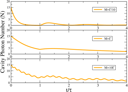
Figure 4: Excitation manifold factorization for different ratios of emitter-cavity strength $M$ versus the decay and feedback strengh $\Gamma$. Our factorization approach allows to extract the feedback feature in the many-photon regime and gives access to a quantum beating corresponding to the coupling strength $M$. Note, in the upper panel, we integrated over a longer absolute time interval to allow for a complete decay of the cavity photon number.

IV Conclusion

We presented a Heisenberg operator method for the description of photon feedback in the quantum limit. Based on a time-delayed feedback equation for the photon coherence, that was derived via the elimination of the feedback reservoir, the dynamics of the system can be calculated by a set of time-correlated expectations values, and can be computed separately for each time interval. Here, the memory of the system leading to the photon feedback is calculated on the fly. As the sets of equations corresponding to a certain time interval only couple to distinctive quantities of the previous and only the previous time interval, memory carrying time-correlators to be stored just grow for the given example linearly with the index of the $\tau$-intervals. This results in an extreme reduction of the numerical effort compared with the incorporation of the reservoir sums, while still bearing all the memory information. The great advantage of the operator method, however, is that it is accessible for the description of more complex systems and with multiple excitations and different statistical properties. As a first outlook, we employed a excitation manifold factorization and showed, that the Heisenberg operator method paves the way to describe efficient and intuitively many-photon quantum feedback. A next step will include a generalization of the feedback dynamics to open, pumped systems.

V Acknowledgments

We would like to thank N. Naumann, M. Kraft and S. Hein for helpful discussions. We acknowledge support from Deutsche Forschungsgemeinschaft through SFB 910 “Control of self-organizing nonlinear systems”.

References

- (1) P. Zoller, T. Beth, D. Binosi, R. Blatt, H. Briegel et al., “Quantum information processing and communication,” Eur. Phys. J. D 36, 203–228 (2005).
- (2) H. Wiseman and G. Milburn, Quantum Measurement and Control (Cambridge University Press, Oxford, 2006).
- (3) T. Brandes, “Feedback between interacting transport channels,” Physical Review E 91, 052149 (2015).
- (4) A. Kiraz, M. Atatüre, and A. Imamoğlu, “Quantum-dot single-photon sources: Prospects for applications in linear optics quantum-information processing,” Physical Review A 69, 032305 (2004).
- (5) J. Wolters, J. Kabuss, A. Knorr, and O. Benson, “Deterministic and robust entanglement of nitrogen-vacancy centers using low-q photonic-crystal cavities,” Physical Review A 89, 060303 (2014).
- (6) C. Sayrin, I. Dotsenko, X. Zhou, B. Peaudecerf, T. Rybarczyk, S. Gleyzes, P. Rouchon, M. Mirrahimi, H. Amini, M. Brune et al., “Real-time quantum feedback prepares and stabilizes photon number states,” Nature 477, 73–77 (2011).
- (7) U. Dorner and P. Zoller, “Laser-driven atoms in half-cavities,” Phys. Rev. A 66, 023816 (2002).
- (8) A. Carmele, J. Kabuss, F. Schulze, S. Reitzenstein, and A. Knorr, “Single photon delayed feedback: a way to stabilize intrinsic quantum cavity electrodynamics,” Physical review letters 110, 013601 (2013).
- (9) A. L. Grimsmo, “Time-delayed quantum feedback control,” arXiv preprint arXiv:1502.06959 (2015).
- (10) H. Pichler and P. Zoller, “Photonic quantum circuits with time delays,” arXiv preprint arXiv:1510.04646 (2015).
- (11) R. Cook and P. Milonni, “Quantum theory of an atom near partially reflecting walls,” Physical Review A 35, 5081 (1987).
- (12) G. Alber, “Photon wave packets and spontaneous decay in a cavity,” Physical Review A 46, R5338 (1992).
- (13) T. Tufarelli, M. Kim, and F. Ciccarello, “Non-markovianity of a quantum emitter in front of a mirror,” Physical Review A 90, 012113 (2014).
- (14) S. M. Hein, F. Schulze, A. Carmele, and A. Knorr, “Optical feedback-enhanced photon entanglement from a biexciton cascade,” Physical review letters 113, 027401 (2014).
- (15) S. Hughes, “Coupled-cavity qed using planar photonic crystals,” Physical review letters 98, 083603 (2007).
- (16) G. Hétet, L. Slodička, M. Hennrich, and R. Blatt, “Single atom as a mirror of an optical cavity,” Physical review letters 107, 133002 (2011).
- (17) F. Albert, C. Hopfmann, S. Reitzenstein, C. Schneider, S. Höfling, L. Worschech, M. Kamp, W. Kinzel, A. Forchel, and I. Kanter, “Observing chaos for quantum-dot microlasers with external feedback,” Nature communications 2, 366 (2011).
- (18) C. Gardiner and P. Zoller, Quantum Noise (Springer, Berlin Heidelberg New York, 1991).
- (19) M. Kira and S. W. Koch, Semiconductor quantum optics (Cambridge University Press, 2011).
- (20) F. Schulze, B. Lingnau, S. M. Hein, A. Carmele, E. Schöll, K. Lüdge, and A. Knorr, “Feedback-induced steady-state light bunching above the lasing threshold,” Physical Review A 89, 041801 (2014).
- (21) R. Lang and K. Kobayashi, “External optical feedback effects on semiconductor injection laser properties,” Quantum Electronics, IEEE Journal of 16, 347–355 (1980).
- (22) M. Kantner, E. Schöll, and S. Yanchuk, “Delay-induced patterns in a two-dimensional lattice of coupled oscillators,” Scientific reports 5 (2015).
- (23) M. Wegert, D. Schwochert, E. Schöll, and K. Lüdge, “Integrated quantum-dot laser devices: modulation stability with electro-optic modulator,” Optical and Quantum Electronics 46, 1337–1344 (2014).
- (24) V. Flunkert, I. Fischer, and E. Schöll, “Dynamics, control and information in delay-coupled systems: an overview,” Philosophical Transactions of the Royal Society of London A: Mathematical, Physical and Engineering Sciences 371, 20120465 (2013).
- (25) A. W. Glaetzle, K. Hammerer, A. Daley, R. Blatt, and P. Zoller, “A single trapped atom in front of an oscillating mirror,” Optics Communications 283, 758–765 (2010).
- (26) C. U. Lei and W.-M. Zhang, “A quantum photonic dissipative transport theory,” Annals of Physics 327, 1408–1433 (2012).
- (27) J. Kabuss, D. O. Krimer, S. Rotter, K. Stannigel, A. Knorr, and A. Carmele, “Analytical study of quantum feedback enhanced rabi oscillations,” arXiv preprint arXiv:1503.05722 (2015).
- (28) V. Flunkert, “Time-delayed feedback control,” in “Delay-Coupled Complex Systems,” (Springer, 2011), pp. 7–10.
- (29) J. Eschner, C. Raab, F. Schmidt-Kaler, and R. Blatt, “Light interference from single atoms and their mirror images,” Nature 413, 495–498 (2001).
- (30) S. M. Hein, F. Schulze, A. Carmele, and A. Knorr, “Entanglement control in quantum networks by quantum-coherent time-delayed feedback,” Physical Review A 91, 052321 (2015).
- (31) A. Carmele, B. Vogell, K. Stannigel, and P. Zoller, “Opto-nanomechanics strongly coupled to a rydberg superatom: coherent versus incoherent dynamics,” New Journal of Physics 16, 063042 (2014).
- (32) W. Kopylov, M. Radonjić, T. Brandes, A. Balaž, and A. Pelster, “Dissipative two-mode tavis-cummings model with time-delayed feedback control,” arXiv preprint arXiv:1507.01811 (2015).
- (33) B. Lingnau, W. W. Chow, E. Schöll, and K. Lüdge, “Feedback and injection locking instabilities in quantum-dot lasers: a microscopically based bifurcation analysis,” New Journal of Physics 15, 093031 (2013).
- (34) C. Gies, J. Wiersig, M. Lorke, and F. Jahnke, “Semiconductor model for quantum-dot-based microcavity lasers,” Physical Review A 75, 013803 (2007).
- (35) H. Leymann, A. Foerster, and J. Wiersig, “Expectation value based equation-of-motion approach for open quantum systems: A general formalism,” Physical Review B 89, 085308 (2014).
- (36) M. Richter, A. Carmele, A. Sitek, and A. Knorr, “Few-photon model of the optical emission of semiconductor quantum dots,” Physical review letters 103, 087407 (2009).