Restricted $f(R)$ Gravity and Its Cosmological Implications

M. Chaichian,^a A. Ghalee,^b J. Klusoň,^c,

^aDepartment of Physics, University of Helsinki, P.O. Box 64,
FI-00014 Helsinki, Finland
^bDepartment of Physics, Tafresh University, Tafresh, Iran
^cDepartment of Theoretical Physics and Astrophysics, Faculty of Science,
Masaryk University, Kotlářská 2, 611 37, Brno, Czech Republic

We investigate the $f(R)$ theory of gravity with broken diffeomorphism due to the change of the coefficient in front of the total divergence term in the ($3+1$)-decomposition of the scalar curvature. We perform the canonical analysis of this theory and show that its consistent, i.e. with no unphysical degrees of freedom, form is equivalent to the low-energy limit of the non-projectable $f(R)$ Hořava-Lifshitz theory of gravity. We also analyze its cosmological solutions and show that the de Sitter solution can be obtained also in the case of this broken symmetry. The consequences of the proposed theory on the asymptotic solutions of a few specific models in the cosmological context are also presented.

1 Introduction

Recent observation data show that $R^{2}-$inflation model for the early Universe is in remarkable agreement with the observations. [1]. Further, the celebrated cosmological constant problem can be also explained in the context of $f(R)$ theories of gravity . It is also possible to find a formulation of $f(R)$ gravity whose solutions of equations of motion capture both the inflation and late time behaviour of the Universe.

It is important to stress that all these cosmological solutions depend only on the time, so that they break the manifest four-dimensional diffeomorphism of General Relativity. Then one can ask the question whether the time asymmetry of Friedmann-Robetson-Walker Universe could be also reproduced by some theory of gravity with restricted symmetry group. Indeed, the celebrated Hořava-Lifshitz (HL) gravity [3, 4, 5] which is an interesting proposal for a renormalizable theory of gravity is based on the idea of the restricted invariance of the theory when the theory is invariant under the so-called foliation preserving diffeomorphism. It turns out that there are two versions of HL gravity, the projectable theory when the lapse depends only on the time and the non-projectable theory with the lapse depending on the spatial coordinates too [3]. It was subsequently shown in [6] that the first versions of non-projectable Hořava-Lifshitz gravity possesses a pathological behaviour since the Hamiltonian constraint is a second-class constraint with itself, which implies that the phase space is odd-dimensional (for further discussions, see [7]). The resolution of this problem was first suggested in [8] and further elaborated in [9, 10], where it was argued that in a theory with broken full diffeomorphism invariance, it is natural to include all the terms which contain the spatial gradients of lapse and which are invariant under spatial diffeomorphism too. Then the Hamiltonian analysis of this theory shows that this Hamiltonian constraint is a second-class constraint with the primary constraint $\pi_{N}\approx 0$, where $\pi_{N}$ is the momentum conjugate to the lapse $N$ [11, 12, 13, 14]. On the other hand, the fact that the number of constraints is less than in General Relativity implies the existence of an extra scalar degrees of freedom.

These considerations suggest that the full diffeomorphism invariance must not be the fundamental symmetry of gravity. In that case it is natural to consider the possibility whether the $f(R)$ theory of gravity, which is not invariant under the full four-dimensional diffeomorphism, can be consistent with the recent cosmological models. There are certainly several ways how to break full diffeomorphism invariance. The most natural way is to generalize HL gravity to its $f(R)-$like form as was done in several papers; see for example [15, 16, 17, 18, 19, 20, 21]. Recently a new interesting proposal for a theory with the broken full diffeomorphism invariance was proposed in [22], which is based on the following simple modification

$$R\rightarrow R_{\Upsilon}\equiv R+(\Upsilon-1)\Xi\ ,$$ (1)

where $\Upsilon$ is a parameter and $\Xi$ is a four-divergence term that appears in the decomposition of the Ricci scalar in four dimensions as [23]

$$R={}^{(3)}R+(K^{ij}K_{ij}-K^{2})+\Xi\ .$$ (2)

Parameter $\Upsilon$ has now meaning as the deformation parameter that in similar context was introduced in case of $f(R)$ HL gravity in [19, 20] while its more physical interpretation will be given in section 5 and in 6. It is important to stress that the last term is a four-divergence and hence for the Einstein-Hilbert action the modification (1) does not make sense, since it gives the boundary contribution that does not affect the equations of motion. On the other hand, it could have non-trivial consequences in the case of $f(R)$ theories of gravity as was shown in [22].

Due to the interesting features of this simple idea (1), we believe it deserves to be studied further. In particular we would like to give a more physical justification for it and see whether the presumptions which were implicitly used in [22] have solid physical grounds. In particular, it is not quite clear whether the Newtonian gauge used there could be implemented in the theory with the broken diffeomorphism invariance. Motivated by these facts, we perform the Hamiltonian analysis of the restricted $f(R)$ gravity. We show, in agreement with [22], that the full diffeomorphism invariance is broken. On the other hand, we show that the naive form of restricted $f(R)$ gravity possesses the same pathological behaviour as the first versions of non-projectable Hořava-Lifshitz gravity, whose description was given above. We resolve this problem in a similar way as in the case of non-projectable HL gravity. More precisely, we show under which conditions the restricted $f(R)$ theory could be considered as a consistent theory from the Hamiltonian point of view. In the first case we impose an additional constraint on the theory. However, a careful Hamiltonian analysis of this version will show that now the theory becomes invariant under the full four-dimensional diffeomorphism and that it reduces to the standard Einstein-Hilbert action with a cosmological constant. The second possibility is to consider an extended version of restricted $f(R)$ gravity when we include the terms containing spatial gradients of the lapse. However, in this case we obtain that this theory could be considered as a low-energy limit of the non-projectable HL theory or gravity. We perform the Hamiltonian analysis of this theory, following [11, 12, 13, 14] and we show that there is an extra scalar degree of freedom, whose consequences on the physical spectrum around FRW background should be taken into account.

Having constructed a consistent modification of $f(R)$ theory of gravity, we proceed to the analysis of its cosmological solutions and we find that the properties of these solutions depend on the value of the parameter $\Upsilon$ that allow us to obtain new solutions which do not exist in the ordinary $f(R)$ theory of gravity.

The structure of this paper is as follows. In the next section we introduce the original formulation of restricted $f(R)$ theory of gravity and perform its Hamiltonian analysis. In section 3 we study a version of this theory with an additional constraint imposed and we show that this theory is equivalent to the ordinary Einstein-Hilbert one. Then in section 4 we propose an extended form of restricted $f(R)$ theory of gravity with the spatial gradients of lapse included. In section 5 we study some cosmological solutions of such a theory. Finally, in section 6, Discussion, we outline our results and suggest a possible extension of the work.

2 Restricted $f(R)$ gravity

Let us consider the $4$-dimensional manifold $\mathcal{M}$ with the coordinates $x^{\mu}\ ,\mu=0,\dots,3$, where $x^{\mu}=(t,\mathbf{x})\ ,\mathbf{x}=(x^{1},x^{2},x^{3})$. We assume that this space-time is endowed with the metric $\hat{g}_{\mu\nu}(x)$ with signature $(-,+,+,+)$. Suppose that $\mathcal{M}$ can be foliated by a family of space-like surfaces $\Sigma_{t}$ defined by $t=x^{0}$. In this work, we are interested in the cosmological implications of our model. So, we will use the flat Friedmann-Robertson-Walker Universe that for which $\Sigma_{t}=\mathbf{R}^{3}$. So, Let $g_{ij},i,j=1,2,3$ denote the metric on $\Sigma_{t}$ with its inverse $g^{ij}$, so that $g_{ij}g^{jk}=\delta_{i}^{k}$. We further introduce the operator $\nabla_{i}$, which is the covariant derivative defined by the metric $g_{ij}$. We introduce the future-pointing unit normal vector $n^{\mu}$ to the surface $\Sigma_{t}$. In ADM variables we have $n^{0}=\sqrt{-\hat{g}^{00}},n^{i}=-\hat{g}^{0i}/\sqrt{-\hat{g}^{00}}$. We also define the lapse function $N=1/\sqrt{-\hat{g}^{00}}$ and the shift function $N^{i}=-\hat{g}^{0i}/\hat{g}^{00}$. In terms of these variables we write the components of the metric $\hat{g}_{\mu\nu}$ as

$$\hat{g}_{00}=-N^{2}+N_{i}g^{ij}N_{j}\ ,\quad\hat{g}_{0i}=N_{i}\ ,\quad\hat{g}_{ij}=g_{ij}\ ,$$

$$\hat{g}^{00}=-\frac{1}{N^{2}}\ ,\quad\hat{g}^{0i}=\frac{N^{i}}{N^{2}}\ ,\quad\hat{g}^{ij}=g^{ij}-\frac{N^{i}N^{j}}{N^{2}}\ .$$

Then it is easy to see that

$$\sqrt{-\det\hat{g}}=N\sqrt{\det g}\ .$$ (4)

Further we define the extrinsic derivative

$$K_{ij}=\frac{1}{2N}(\partial_{t}g_{ij}-\nabla_{i}N_{j}-\nabla_{j}N_{i})\ .$$ (5)

It is well known that the components of the Riemann tensor can be written in terms of ADM variables . For example, in the case of Riemann curvature we have

$$R = K^{ij}K_{ij}-K^{2}+{}^{(3)}R+\frac{2}{\sqrt{-\hat{g}}}\partial_{\mu}(\sqrt{-\hat{g}}n^{\mu}K)-\frac{2}{\sqrt{g}N}\partial_{i}(\sqrt{g}g^{ij}\partial_{j}N)$$

$$= K^{ij}K_{ij}-K^{2}+{}^{(3)}R+\Xi\ .$$

The restricted $f(R)$ gravity is based on the idea that we modify $R$ in the following way

$$R\rightarrow R+(\Upsilon-1)\Xi\ ,$$ (7)

where $\Upsilon$ is a constant. Then we consider the action in the form

$$S_{f(R)}=\frac{1}{\kappa^{2}}\int dtd^{3}\mathbf{x}\sqrt{g}Nf(R+(\Upsilon-1)\Xi)\ .$$ (8)

Note that, since $\Sigma_{t}=\mathbf{R}^{3}$ has no boundary, we have not considered any boundary term in the action.
Our goal is to perform the Hamiltonian analysis of the action (8). We introduce two auxiliary scalar fields A and B and rewrite the action in the equivalent form

$$S_{f(R)}=\frac{1}{\kappa^{2}}\int dtd^{3}\mathbf{x}\sqrt{g}N(f(A)+B(R+(\Upsilon-1)\Xi-A))\ .$$ (9)

It can be easily seen that the action (9) is equivalent to the action (8) when we solve the equation of motion for $B$ and gives $A=R+(\Upsilon-1)\Xi$. Inserting back this result into (9) we obtain (8). Now using the explicit form of $\Xi$ we can rewrite the action (9) into the form

$$S_{f(R)} = \frac{1}{\kappa^{2}}\int dtd^{3}\mathbf{x}\left(\sqrt{g}NB(K_{ij}\mathcal{G}^{ijkl}K_{kl}+{}^{(3)}R-A)\right.$$

$$+ \left.\sqrt{g}Nf(A)-2\Upsilon\sqrt{g}N\nabla_{n}Bg^{ij}K_{ji}+2\Upsilon\partial_{i}B\sqrt{g}g^{ij}\partial_{j}N\right)\ ,$$

where we have introduced the de Witt metric $\mathcal{G}^{ijkl}$

$$\mathcal{G}^{ijkl}=\frac{1}{2}(g^{ik}g^{jl}+g^{il}g^{jk})-g^{ij}g^{kl}\ ,$$ (11)

and where

$$\nabla_{n}B=\frac{1}{N}(\partial_{t}B-N^{i}\partial_{i}B)\ .$$ (12)

From (2) we find the conjugate momenta

$$\pi^{ij} = \frac{1}{\kappa^{2}}\sqrt{g}B\mathcal{G}^{ijkl}K_{kl}-\frac{1}{\kappa^{2}}\Upsilon\sqrt{g}\nabla_{n}Bg^{ij}\ ,\quad\pi_{N}\approx 0\ ,\quad\pi_{i}\approx 0\ ,$$

$$p_{B} = -\frac{2}{\kappa^{2}}\Upsilon\sqrt{g}K\ ,\quad p_{A}\approx 0\ .$$

Then it is easy to find Hamiltonian density in the form

$$\mathcal{H}=\partial_{t}g_{ij}\pi^{ij}+p_{B}\partial_{t}B-\mathcal{L}=N\mathcal{H}_{T}+N^{i}\mathcal{H}_{i}\ ,$$

where

$$\mathcal{H}_{T} = \frac{\kappa^{2}}{\sqrt{g}B}\pi^{ij}g_{ik}g_{jl}\pi^{kl}-\frac{\kappa^{2}}{3B\sqrt{g}}\pi^{2}-\frac{\kappa^{2}}{3\sqrt{g}\Upsilon}p_{B}\pi$$

$$+ \frac{\kappa^{2}}{6\Upsilon^{2}\sqrt{g}}Bp_{B}^{2}-\frac{\sqrt{g}}{\kappa^{2}}B({}^{(3)}R-A)-\frac{1}{\kappa^{2}}\sqrt{g}f(A)+\frac{2\Upsilon}{\kappa^{2}}\partial_{i}[\sqrt{g}g^{ij}\partial_{j}B]\ ,$$

$$\mathcal{H}_{i} = -2g_{ik}\nabla_{j}\pi^{jk}+p_{B}\partial_{i}B\ .$$

Now the requirement of the preservation of the primary constraints $\pi_{N}(\mathbf{x})\approx 0,\pi_{i}(\mathbf{x})\approx 0$ and $p_{A}(\mathbf{x})\approx 0$, implies the following secondary ones

$$\partial_{t}\pi_{N}(\mathbf{x}) = \left\{\pi_{N}(\mathbf{x}),H\right\}=\mathcal{H}_{T}(\mathbf{x})\approx 0\ ,$$

$$\partial_{t}p_{i}(\mathbf{x}) = \left\{p_{i}(\mathbf{x}),H\right\}=-\mathcal{H}_{i}(\mathbf{x})\approx 0\ ,$$

$$\partial_{t}p_{A}(\mathbf{x}) = -\frac{1}{\kappa^{2}}\sqrt{g}B+\frac{1}{\kappa^{2}}\sqrt{g}f^{\prime}(A)\equiv G_{A}(\mathbf{x})\approx 0\ .$$

Since $\left\{p_{A}(\mathbf{x}),G_{A}(\mathbf{y})\right\}=-\frac{1}{\kappa^{2}}\sqrt{g}f^{\prime\prime}(A)\delta(\mathbf{x}-\mathbf{y})$, we see that $(p_{A},G_{A})$ are the second-class constraints and hence can be explicitly solved. In solving the first one, we set $p_{A}$ strongly zero, while solving the second one, we find $f^{\prime}(A)=B$. Assuming that $f^{\prime}$ is invertible, we can express $A$ as a function of $B$ so that $A=\Psi(B)$ for some function $\Psi$. Finally, since $\left\{\pi^{ij},p_{A}\right\}=\left\{g_{ij},p_{A}\right\}=0$, we see that the Dirac brackets between the canonical variables coincide with the Poisson brackets.

Now we proceed to the analysis of the preservation of all constraints. We begin with the constraint $\mathcal{H}_{i}$, which we modify in the following way

$$\tilde{\mathcal{H}}_{i}=\mathcal{H}_{i}+p_{A}\partial_{i}A=-2g_{ik}\nabla_{j}\pi^{jk}+p_{A}\partial_{i}A+p_{B}\partial_{i}B.\$$ (17)

It is convenient to define the smeared form of these fields

$$\mathbf{T}_{S}(N^{i})=\int d^{3}\mathbf{x}N^{i}\tilde{\mathcal{H}}_{i}\ .$$ (18)

The reason why one considers the smeared forms( i.e. takes the constraints integrated by multiplying them with some smooth functions) is to easily deal with the distributions, which is the usual and rigorous way, since the point-wise constraints are distributions and in particular they contain the delta functions and their derivatives. In principle, one can perform all the calculations without their smeared forms, but then more care has to be taken. Then it is easy to show that $\mathbf{T}_{S}(N^{i})$ are the generators of the spatial diffeomorphism and that they are the first-class constraints. We rather focus on the analysis of the Hamiltonian constraint. It is also convenient to introduce as well the smeared form of the Hamiltonian constraint

$$\mathbf{T}_{T}(N)=\int d^{3}\mathbf{x}N\mathcal{H}_{T}\ .$$ (19)

Our goal is to perform the calculation of the Poisson bracket between the smeared forms of the Hamiltonian constraints $\left\{\mathbf{T}_{T}(N),\mathbf{T}_{T}(M)\right\}$. Then after some careful calculations we find

$$\left\{\mathbf{T}_{T}(N),\mathbf{T}_{T}(M)\right\} = \mathbf{T}_{S}((N\nabla_{j}M-M\nabla_{j}N)g^{ji})$$

$$+ \frac{4}{3}(1-\Upsilon)\int d^{3}\mathbf{x}(M\nabla_{i}N-N\nabla_{i}M)\frac{\pi}{B}\nabla^{i}B$$

$$+ 4(1-\Upsilon)\int d^{3}\mathbf{x}(N\nabla_{i}M-M\nabla_{i}N)\frac{\pi^{ij}}{B}\nabla_{j}B$$

$$+ \frac{\Upsilon-1}{3\Upsilon}\int d^{3}\mathbf{x}(N\nabla_{i}M-M\nabla_{i}N)p_{B}\nabla^{i}B\ .$$

The expression on the first line is the standard form of the Poisson bracket between smeared forms of Hamiltonian constraint for the full diffeomorphism invariant theory. On the other, the additional terms in (2) which are proportional to $\Upsilon-1$ do not vanish on the constraint surface and explicitly show the breaking of the full diffeomorphism invariance. Moreover, this result suggests that we have a theory where $\mathcal{H}_{T}$ is a second-class constraint, which is the situation that is known from the analysis of the first versions of non-projectable Hořava-Lifshitz gravity [6, 7]. As was argued there, the existence of one second-class constraint implies that the dimension of the physical phase space is odd, what should not be. It turns out that there are two possibilities how to resolve this puzzle. The first one is based on the observation that the right side of the Poisson bracket (2) vanishes on the constraint surface when $\partial_{i}B=0$. We will discuss this case in the next section.

3 Projectable restricted $f(R)$ gravity

To proceed with the condition $\partial_{i}B=0$, we introduce the following decomposition of the scalar field $B$

$$B=\tilde{B}+B_{0}\ ,$$ (21)

where

$$B_{0}=\frac{1}{\int d^{3}\mathbf{x}\sqrt{g}}\int d^{3}\mathbf{x}\sqrt{g}B$$ (22)

and hence $\int d^{3}\mathbf{x}\sqrt{g}\tilde{B}=0$. Then the condition $\partial_{i}B=0$ implies $\tilde{B}=K(t)$ for any function $K(t)$. On the other hand, since $\int d^{3}\mathbf{x}\sqrt{g}\tilde{B}=0$, we obtain that $K(t)=0$. In other words, the condition $\partial_{i}B=0$ is equivalent to the constraint

$$\Phi_{I}\equiv\tilde{B}\approx 0\ .$$ (23)

Obviously, we have to ensure that this constraint is also preserved during the time evolution of the system. To do that, we also decompose the momenta $p_{B}$ as

$$p_{B}=\tilde{p}_{B}+\frac{\sqrt{g}}{\int d^{3}\mathbf{x}\sqrt{g}}P_{B}\ ,\quad P_{B}=\int d^{3}\mathbf{x}p_{B}\ ,\quad\int d^{3}\mathbf{x}\tilde{p}_{B}=0\ ,$$ (24)

where we have the following Poisson brackets

$$\left\{B_{0},P_{B}\right\}=1\ ,\quad\left\{\tilde{p}_{B}(\mathbf{x}),B_{0}\right\}=\left\{\tilde{B}(\mathbf{x}),P_{B}\right\}=0\ ,\quad$$

$$\left\{\tilde{B}(\mathbf{x}),\tilde{p}_{B}(\mathbf{y})\right\}=\delta(\mathbf{x}-\mathbf{y})-\frac{\sqrt{g}(\mathbf{y})}{\int d^{3}\mathbf{z}\sqrt{g}(\mathbf{z})}\ .$$

Finally we have to analyze the requirement of the preservation of the constraint $\Phi_{I}\approx 0$

$$\partial_{t}\Phi_{I} =\left\{\Phi_{I}(\mathbf{x}),H\right\}$$

$$= \int d^{3}\mathbf{y}N\frac{\kappa^{2}}{3\sqrt{g}}\left(\tilde{p}_{B}+\frac{\sqrt{g}}{\int d^{3}\mathbf{z}\sqrt{g}}P_{B}-\Upsilon\pi\right)\left(\delta(\mathbf{x}-\mathbf{y})-\frac{\sqrt{g}(\mathbf{y})}{\int d^{3}\mathbf{z}\sqrt{g}(\mathbf{z})}\right)\ .$$

In order to preserve the constraint $\Phi_{I}\approx 0$, it is natural to impose the following constraint

$$\Phi_{II}\equiv\frac{1}{\sqrt{g}}\left[\tilde{p}_{B}+\frac{\sqrt{g}}{\int d^{3}\mathbf{z}\sqrt{g}}P_{B}-\Upsilon\pi\right]\approx 0\ .$$ (27)

Now thanks to the Poisson bracket (3), we see that there exists a non-zero Poisson bracket $\left\{\Phi_{I}(\mathbf{x}),\Phi_{II}(\mathbf{y})\right\}\neq 0$, so that they are the second-class constraints. We recall that there are still two additional second-class constraints $p_{A}\approx 0,G_{A}\approx 0$. Solving these second-class constraints, we obtain the Hamiltonian constraint $\mathcal{H}_{T}$ in the form

$$\mathcal{H}_{T}=\frac{\kappa^{2}}{\sqrt{g}B_{0}}\left(\pi^{ij}g_{ik}g_{jl}-\frac{1}{2}\pi^{2}\right)-\frac{\sqrt{g}}{\kappa^{2}}B_{0}({}^{(3)}R-A)-\frac{1}{\kappa^{2}}\sqrt{g}f(B_{0})\ ,$$

where we have also solved $G_{A}$ for $A$ as $A=\Psi(B_{0})$. Finally, note that $\mathcal{H}_{T}$ does not depend on $P_{B}$ and hence $B_{0}$ is constant on-shell and we see that (3) corresponds to the Hamiltonian constraint of General Relativity with a cosmological constant when $B_{0}$ is absorbed into the definition of $\kappa$. In other words, the condition $\tilde{B}\approx 0$ implies that the above considered restricted $f(R)$ gravity is equivalent to General Relativity. For that reason we have to consider the second possibility when we abandon the requirement that $\mathcal{H}_{T}$ is a first-class constraint.

4 Extended Form of Restricted $f(R)$ gravity

In this section we show how to resolve the problem with the naive existence of the second-class constraint $\mathcal{H}_{T}$ in the restricted $f(R)$ gravity. The resolution of this puzzle is based on the fact that whenever we accept that some theory is not invariant under the full diffeomorphism, it is natural to include all the terms that are compatible with the spatial diffeomorphism in the definition of the action. In other words, we should consider a more general version of restricted $f(R)$ gravity that is similar to the so-named healthy extension of HL gravity [8, 9, 10]. In this section we consider such a modification of the restricted $f(R)$ gravity when we include in the action additional terms which are invariant under spatial diffeomorphism. Following the discussion performed in the case of HL gravity, we also replace the de Witt metric by a generalized de Witt metric which has the form [3]

$$\tilde{\mathcal{G}}^{ijkl} = \frac{1}{2}(g^{ik}g^{jl}+g^{il}g^{jk})-\lambda g^{ij}g^{kl}\ ,\quad\lambda\neq\frac{1}{3}\ ,$$

$$\tilde{\mathcal{G}}_{ijkl} = \frac{1}{2}(g_{ik}g_{jl}+g_{il}g_{jk})-\frac{\lambda}{3\lambda-1}g_{ij}g_{kl}\ .$$

More importantly, due to the fact that the theory is not invariant under the full four-dimensional diffeomorphism, it is natural to include the vector $a_{i}=\frac{\partial_{i}N}{N}$ into the definition of the action. In other words, our extended form of restricted $f(R)$ gravity arises when we perform the replacement

$$R\rightarrow K_{ij}\tilde{\mathcal{G}}^{ijkl}K_{kl}+{}^{(3)}R+\Upsilon\Xi+\gamma_{1}a_{i}a^{i}+\gamma_{2}{}^{(3)}R^{ij}a_{i}a_{j}\ ,$$ (30)

where $\gamma_{1},\gamma_{2}$ are the corresponding coupling constants. Then the action with auxiliary fields $A$ and $B$ has the form

$$\tilde{S}_{f(R)} = \frac{1}{\kappa^{2}}\int dtd^{3}\mathbf{x}\left(\sqrt{g}NB(K_{ij}\tilde{\mathcal{G}}^{ijkl}K_{kl}+{}^{(3)}R+\gamma_{1}a_{i}a^{i}+\gamma_{2}{}^{(3)}R^{ij}a_{i}a_{j}-A)\right.$$

$$+ \left.\sqrt{g}Nf(A)-2\Upsilon\sqrt{g}N\nabla_{n}Bg^{ij}K_{ji}+2\Upsilon\partial_{i}B\sqrt{g}g^{ij}\partial_{j}N\right)\ .$$

Now we are ready to proceed to the Hamiltonian analysis of the theory defined by the action (4). Following the same logic as in section (2) we find the Hamiltonian density in the form

$$\mathcal{H}=\partial_{t}g_{ij}\pi^{ij}+p_{B}\partial_{t}B-\mathcal{L}=N\mathcal{H}_{T}+N^{i}\mathcal{H}_{i}\ ,$$

where

$$\mathcal{H}_{T} = \frac{\kappa^{2}}{\sqrt{g}B}\pi^{ij}g_{ik}g_{jl}\pi^{kl}-\frac{\kappa^{2}}{3\sqrt{g}}\pi^{2}-\frac{\kappa^{2}}{3\sqrt{g}\Upsilon}p_{B}\pi-\frac{(1-3\lambda)\kappa^{2}}{12\Upsilon^{2}\sqrt{g}}Bp_{B}^{2}$$

$$- \frac{\sqrt{g}}{\kappa^{2}}B({}^{(3)}R+\gamma_{1}a_{i}a^{i}+\gamma_{2}{}^{(3)}R^{ij}a_{i}a_{j}-A)-\frac{1}{\kappa^{2}}\sqrt{g}f(A)+\frac{2\Upsilon}{\kappa^{2}}\partial_{i}[\sqrt{g}g^{ij}\partial_{j}B]\ ,$$

$$\mathcal{H}_{i} = -2g_{ik}\nabla_{j}\pi^{jk}+p_{B}\partial_{i}B\ .$$

Note that this form of the Hamiltonian constraint is in agreement with the constraint (up to the potential term and terms containing $a_{i}$) found in [21].

It is also very important to identify the global constraints which are related to the action (4). In fact, it is easy to see that there is a primary global constraint [12]

$$\Pi_{N}=\int d^{3}\mathbf{x}\pi_{N}N\ ,$$ (34)

which has the following non-zero Poisson brackets with $N$ and $\pi_{N}$

$$\left\{\Pi_{N},a_{i}(\mathbf{x})\right\}=0\ ,\quad\left\{\Pi_{N},N(\mathbf{x})\right\}=-N(\mathbf{x})\ ,\quad\left\{\Pi_{N},\pi_{N}(\mathbf{x})\right\}=\pi_{N}(\mathbf{x})\ .$$ (35)

We show below that $\Pi_{N}$ is a first-class constraint. It turns out that we have to be careful with the definition of the local and global constraints. Following the notation used in [14], we define a local constraint as

$$\tilde{\pi}_{N}(\mathbf{x})=\pi_{N}(\mathbf{x})-\frac{\sqrt{g}(\mathbf{x})}{\int d^{3}\mathbf{x}N\sqrt{g}}\Pi_{N}\ .$$ (36)

Saying it differently, we decompose the constraint $\pi_{N}(\mathbf{x})$ into the local and global constraints, $\tilde{\pi}_{N}(\mathbf{x})$ and $\Pi_{N}$, respectively and we denote it symbolically by ”$\infty^{3}-1$” local constraints $\tilde{\pi}_{N}(\mathbf{x})$, as follows from the fact that the constraint $\tilde{\pi}_{N}$ obeys the equation

$$\int d^{3}\mathbf{x}N(\mathbf{x})\tilde{\pi}_{N}(\mathbf{x})=0\ .$$ (37)

Now together with the global constraint $\Pi_{N}$, we have a total number of ”$\infty^{3}$” constraints, which is the same as the number of the original constraints $\pi_{N}$.

In summary, the Hamiltonian with the primary constraints included has the form

$$H=\Pi_{N}+\int d^{3}\mathbf{x}(N\mathcal{H}_{T}+N^{i}\tilde{\mathcal{H}}_{i}+v_{N}\tilde{\pi}_{N}+v^{i}\pi_{i}+v_{A}p_{A})\ \ .$$ (38)

Now we have to proceed to the analysis of the preservation of the primary constraints $\tilde{\pi}_{N}\approx 0,\pi_{i}\approx 0\ ,p_{A}\approx 0$ and $\Pi_{N}$. In the case of the constraint $\Pi_{N}\approx 0$ we obtain

$$\partial_{t}\Pi_{N}=\left\{\Pi_{N},H\right\}=-\int d^{3}\mathbf{x}N\mathcal{H}_{T}\equiv-\Pi_{T}\approx 0\ ,$$ (39)

where $\Pi_{T}=\int d^{3}\mathbf{x}N\mathcal{H}_{T}\approx 0$ is the global Hamiltonian constraint [12]. The requirement of the preservation of the constraints $\pi_{i}\approx 0$ and $p_{A}\approx 0$ implies the same constraints as in the second section, namely $\mathcal{H}_{i}$ and $G_{A}$. Finally, the requirement of the preservation of the constraint $\tilde{\pi}_{N}\approx 0$ implies

$$\partial_{t}\tilde{\pi}_{N}(\mathbf{x}) = \left\{\tilde{\pi}_{N}(\mathbf{x}),H\right\}$$

$$= -\mathcal{H}_{T}-\frac{2}{\kappa^{2}}\sqrt{g}[B(\gamma_{1}a_{i}a^{i}+\gamma_{2}R_{ij}a^{i}a^{j})+\nabla_{i}[B\gamma_{1}a^{i}+\gamma_{2}R_{kl}g^{ki}g^{lj}a_{j}]]\equiv-\mathcal{C}(\mathbf{x})\ .$$

However, not all the $\mathcal{C}(\mathbf{x})$ are independent since we have

$$\int d^{3}\mathbf{x}N\mathcal{C}=\Pi_{T}\ ,$$ (41)

where we have ignored the boundary terms. Then we see that it is natural to introduce ”$\infty^{3}-1$” independent constraints $\tilde{\mathcal{C}}(\mathbf{x})\approx 0$ defined as

$$\tilde{\mathcal{C}}(\mathbf{x})=\mathcal{C}(\mathbf{x})-\frac{\sqrt{g}(\mathbf{x})}{\int d^{3}\mathbf{y}N\sqrt{g}}\Pi_{T}\ ,$$ (42)

which obey the relation

$$\int d^{3}\mathbf{x}N(\mathbf{x})\tilde{\mathcal{C}}(\mathbf{x})=0\ .$$ (43)

In summary, the total Hamiltonian with all constraints included has the form

$$H_{T}=\Pi_{T}+\Pi_{N}+\int d^{3}\mathbf{x}(N\tilde{\mathcal{C}}+N^{i}\tilde{\mathcal{H}}_{i}+v_{N}\tilde{\pi}_{N}+v^{i}\pi_{i}+v_{A}p_{A}+\Gamma^{A}G_{A})\ .$$ (44)

Now we are ready to study the preservation of all the constraints. It is easy to show that $\Pi_{N},\Pi_{T}$ are global first class constraints while $\tilde{\mathcal{H}}_{i}$ are local first class constraints. On the other hand $(\tilde{\pi}_{N},p_{A},\tilde{\mathcal{C}},G_{A})$ and the second class constraints. In summary, we have the following picture of the restricted $f(R)$ gravity. This is a theory which is invariant under the spatial diffeomorphism with three local first-class constraints corresponding to this symmetry. We also have four second-class constraints. Solving these constraints, we can express $A,p_{A}$ and $\tilde{\pi}_{N}$ and $N$ as functions of the dynamical variables. The physical phase space of this theory is spanned by $g_{ij},\pi^{ij}$, where six of these degrees of freedom can be eliminated by gauge fixing of the diffeomorphism constraints $\tilde{\mathcal{H}}_{i}$. We see that there is a scalar graviton degree of freedom as in the non-projectable HL gravity with all its consequences on the physical properties of this theory. Finally, there is also a scalar degree of freedom $B$ with conjugate momenta $p_{B}$, as in the ordinary $f(R)$ theory of gravity.

5 Cosmological Aspects of the Theory

In this section we study the restricted $f(R)$ theory of gravity in the cosmological context for which the FRW metric is the preferred coordinate system of the Universe. We will consider mechanisms that lead to an accelerated expansion phase.
To show the mass scale of modified gravity $M$, it is convenient to consider the usual $f(R)$-gravity as

$$\frac{f(R)}{\kappa^{2}}=\frac{M_{P}^{2}R}{2}+M^{4}\tilde{f}\left(\frac{R}{M^{2}}\right).$$ (45)

We also assume that the metric has the standard flat FRW form

$$ds^{2}=-N^{2}(t)dt^{2}+a(t)^{2}dx^{i}dx^{j}\delta_{ij}\ ,$$ (46)

where $a=a(t)$ is the scale factor. Then the right-hand side of (30) takes the following form

$$R_{\Upsilon}\equiv A+\Upsilon\Xi\ ,$$ (47)

where

$$\Xi=-6\frac{H\dot{N}}{N^{3}}+6\frac{\dot{H}}{N^{2}}+18\frac{H^{2}}{N^{2}}\hskip 2.27626pt,\quad A\equiv(1-3\lambda)\frac{3H^{2}}{N^{2}}\ ,$$ (48)

and the Hubble parameter is defined as $H\equiv\frac{\dot{a}}{a}$.

If we now insert (47) and (48) into (45) and perform variation of the action (45) with respect to $N$, we obtain

$$\begin{split}&\frac{3}{2}(3\lambda-1)M_{P}^{2}H^{2}+M^{4}\tilde{f}+6(3\lambda-1-\Upsilon)M^{2}H^{2}\tilde{f}^{\prime}-\Upsilon M^{2}R\tilde{f}^{\prime}\\ &+72\Upsilon(\Upsilon-1)H^{2}\dot{H}\tilde{f}^{\prime\prime}+6\Upsilon^{2}H\dot{R}\tilde{f}^{\prime\prime}=0\ ,\end{split}$$ (49)

where we have set $N=1$ and $R=6\dot{H}+12H^{2}$ . Prime denotes the derivative with respect to the argument of $\tilde{f}$, which is defined as

$$\tilde{f}\equiv\tilde{f}\left(\frac{R_{\Upsilon}}{M^{2}}\right).$$ (50)

The other equation, which is obtained by variation of the action with respect to the scale factor, is not an independent equation .

We see that the structure and properties of the (49) depend on the fact whether $\Upsilon$ is equal to zero or not. In particular, if we take $\Upsilon=0$, the terms with time derivatives vanish in eq.(49). We perform the analysis of this special case later and rather focus on the more standard case when $\Upsilon\neq 0$.

5.1 $\Upsilon\neq 0$ case

Since the effective equation of state parameter is defined as

$$w_{eff}\equiv-1-\frac{2}{3}\frac{\dot{H}}{H^{2}}\ ,$$ (51)

there exist different mechanisms to obtain $w_{eff}<-1/3$, as follows:

• The de Sitter solution: The obvious way to have $w_{eff}<-1/3$ is to require that a constant Hubble parameter $H_{*}$ is a solution of (49)

  $$\frac{3}{2}(3\lambda-1)M_{P}^{2}H_{*}^{2}+M^{4}\tilde{f}_{*}+6(3\lambda-1-3\Upsilon)M^{2}H_{*}^{2}\tilde{f}_{*}^{\prime}=0\ ,$$ (52)

  where

  $$\tilde{f}_{*}\equiv\tilde{f}\left(\frac{R_{\Upsilon}^{*}}{M^{2}}\right)=\tilde{f}\left[(1-3\lambda)\frac{3H_{*}^{2}}{M^{2}}+18\frac{\Upsilon}{M^{2}}H_{*}^{2}\right].$$ (53)

  If eq.(52) has at least one solution, we should determine whether this solution is stable or unstable. In order to check the stability, we consider a small perturbation $\delta H(t)$ around the solution as

  $$H(t)=H_{*}+\delta H(t).$$ (54)

  Inserting this expression into eq.(49) and performing its linearization, we obtain

  $$\Upsilon^{2}\delta\ddot{H}+3H_{*}\Upsilon(\Upsilon+\lambda-1)\delta\dot{H}+\Gamma_{\lambda}H_{*}^{2}\delta H(t)=0\ ,$$ (55)

  where

  $$\Gamma_{\lambda}\equiv(3\lambda-1)\left(\frac{M_{P}^{2}}{12H_{*}^{2}\tilde{f}_{*}^{\prime\prime}}+\frac{M^{2}}{6H_{*}^{2}}\frac{\tilde{f}_{*}^{\prime}}{\tilde{f}_{*}^{\prime\prime}}\right)+(3\lambda-1-3\Upsilon)(6\Upsilon-3\lambda+1)\ ,$$ (56)

  and where we have used (52). eq.(55) has a solution $\delta H\propto\exp(\chi H_{*}t$), where $\chi$ is solution of the following equation

  $$\Upsilon^{2}\chi^{2}+3\Upsilon(\Upsilon+\lambda-1)\chi+\Gamma_{\lambda}=0\ .$$ (57)

  Thus, it is clear that the stability of the de Sitter depends both on the specific form of the theory and on the values of the parameters.
  To compare the new features of the theory with the usual $f(R)$ gravity, let us henceforth in this section take $\lambda=1$. Then we see that the second term in eq.(57) is positive and we have the following possibilities:
  For

  $$\Gamma\equiv\Gamma_{\lambda=1}>0\ ,$$ (58)

  the real part of the solutions or the real solutions are negative. Thus, in this case the Sitter solution is an attractor solution and is suitable for the late-time cosmology. As a check we note that for $\Upsilon=1$, both (52) and (56) have the same form as the corresponding relations derived in [25].

  For

  $$\Gamma<0\$$ (59)

  the equation (57) has two real solutions, where one of them, $\chi_{+}$, is positive and the second one, $\chi_{-}$, is negative. Then de Sitter solution is unstable since at late times we have

  $$\delta H(t)\propto\exp(\chi_{+}H_{*}t)\ .$$ (60)

  In the original Starobinsky’s model [26] and as well in the context of asymptotically safe inflation [27], the unstable de Sitter solution has been used to produce inflationary era for the early Universe. The mechanism is based on the fact that during the time interval $\delta t$, where $\chi_{+}H_{*}\delta t<1$, the solution is close to the de Sitter solution. Thus, one can define the number of $e-$foldings as $N_{e}=H_{*}\delta t$. In order to solve the horizon problem, we take $N_{e}=60$ which gives an upper bound on $\chi_{+}$ and hence on $\Upsilon$ too.

  Specifically, let us consider the following form of the function $\tilde{f}$

  $$\tilde{f}(R/M^{2})=-M^{2n}/R^{n}\ ,$$ (61)

  where $n$ is a positive number [28]. Then using (30), we find that the restricted version of this theory is given by

  $$\tilde{f}=\frac{-M^{2n}}{[R+(\Upsilon-1)\Xi)]^{n}},$$ (62)

  so that from (52) we obtain

  $$H_{*}^{2n+2}=\frac{M^{2n+4}}{M_{P}^{2}}\frac{12\Upsilon-6}{(18\Upsilon-6)^{n+1}}\ .$$ (63)

  Inserting (63) into (56), we find

  $$\Gamma=-2\frac{n+1}{n}(1-3\Upsilon)^{2}\ .$$ (64)

  Therefore, for any $\Upsilon$ and $n$ the de Sitter solution is unstable. Note also that for $\Upsilon=1$ our discussion is in agreement with [28].
  To see another example, consider $R^{2}$-gravity. In this case (52) gives

  $$H_{*}^{2}=\frac{M_{P}^{2}}{36(1+3\Upsilon^{2}-4\Upsilon)}\ .$$ (65)

  It is important to stress that there is no de Sitter solution in the case when $\Upsilon=1$, while it exists when either $\Upsilon>1$ or $\Upsilon<1/3$, as is shown in Fig. 1.

  

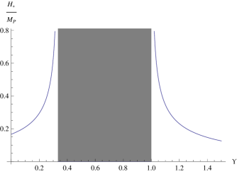
  Figure 1: $\frac{H_{*}}{M_{P}}$ vs $\Upsilon$ for eq.(65). There is no de Sitter solution in the gray region. As is clear, the de Sitter solution can be produced by breaking the diffeomorphism symmetry.

  For such values of parameters eqs. (56) and (65) give

  $$\Gamma=-3(1+3\Upsilon^{2}-4\Upsilon)\ .$$ (66)

  Thus, all the de Sitter solutions are unstable. Using (66), we derive the positive solution of (57) in the form

  $$\chi_{+}=-\frac{3}{2}+\sqrt{\frac{45}{4}+\frac{3}{\Upsilon^{2}}-\frac{12}{\Upsilon}}\ .$$ (67)

  So, in order to have $\chi_{+}<1/N_{e}\sim 0.01$, we have to take $1<\Upsilon<1.1$ or $\frac{1}{3}-0.1<\Upsilon<\frac{1}{3}$  .
  

• Power-Law Acceleration: We have shown that for $\tilde{f}\sim R^{-n}$ the de Sitter solution is not stable. On the other hand, it was shown in [28] that there exists another mechanism which produces the accelerated expansion phase. We would like to investigate this mechanism in the context of restricted the $f(R)$ gravity, while we proceed in a slightly different from [28] way. Of course our procedure is valid for $\Upsilon=1$ and we clarify this point in [29].
  By inserting (62) into (49), we obtain the following form of the equation

  $$\begin{split}&(1+n\Upsilon)(-1+3\Upsilon+\Upsilon\frac{\dot{H}}{H^{2}})^{2}-n(2-\Upsilon)(-1+3\Upsilon+\Upsilon\frac{\dot{H}}{H^{2}})\\ &+2\Upsilon(\Upsilon-1)n(n+1)\frac{\dot{H}}{H^{2}}+n(n+1)\Upsilon^{2}(\frac{\ddot{H}}{H^{3}}+4\frac{\dot{H}}{H^{2}})\\ &=\frac{3M_{P}^{2}}{M^{4+2n}}H^{2+2n}(-6+18\Upsilon+6\Upsilon\frac{\dot{H}}{H^{2}})^{n}.\end{split}$$ (68)

  Since there is not any stable de Sitter solution, as time passes the right-hand side of (68) decreases. So, for the late-time cosmology, one can drop this term. But, without this term, the equation admits a power-law solution as $a\propto t^{1/\epsilon}$, where $\epsilon>0$ is determined from the following equation

  $$\begin{split}&\epsilon^{2}\Upsilon^{2}(1+n\Upsilon+2n^{2}+2n)+(3\Upsilon-1)(-1-2n+3\Upsilon+3n\Upsilon^{2})\\ &-\epsilon\Upsilon(-2+5n\Upsilon+6\Upsilon+6n\Upsilon^{2}+6n^{2}\Upsilon-2n^{2}-4n)=0\ .\end{split}$$ (69)

  This equation has two solutions. In one of them the denominator of eq.(62) approaches to zero and we will discuss it afterwards. The other solution is

  $$\epsilon=\frac{3n\Upsilon^{2}+3\Upsilon-2n-1}{\Upsilon(1+2n+2n^{2}+n\Upsilon)}\ .$$ (70)

  For the latter solution the effective equation of state parameter can be given as

  $$w_{eff}=-1+\frac{2}{3}\frac{3n\Upsilon^{2}+3\Upsilon-2n-1}{\Upsilon(1+2n+2n^{2}+n\Upsilon)}\ .$$ (71)

  Note again that for $\Upsilon=1$ this result agrees with the corresponding relation in [28]. We also see that, since $\epsilon>0$, we can obtain constraints on $\Upsilon$ from eq.(70). For example if we take $n=1$, we obtain

  $$\epsilon=3\frac{(\Upsilon^{2}+\Upsilon-1)}{\Upsilon(5+\Upsilon)}\ .$$ (72)

  Therefore, in order to impose $\epsilon>0$, we should take $\Upsilon>0.61$.
  To show the implication of the theory, let us compare two situations. In the first case, we take $\Upsilon=1$ which gives

  $$w_{eff}|_{\Upsilon=1}=-1+\frac{2}{3}\frac{n+2}{(2n^{2}+3n+1)}\ .$$ (73)

  So, for $n=1$ we have $w_{eff}|_{\Upsilon=1}=-2/3$, which is not in agreement with the recent observations [1]. Of course, as argued in [28], one can increase $n$ to fit the model with the observations as is shown in Fig. 2. For example, if we require $w_{eff}|_{\Upsilon=1}=-0.997$ to reconcile the model with the recent observations [1], we should take $n=100$, which may not be interesting.
  

  On the other hand, let us now consider $n=1$ and leave $\Upsilon$ arbitrary. Then from (70) we obtain

  $$w_{eff}|_{n=1}=-1+2\frac{\Upsilon^{2}+\Upsilon-1}{\Upsilon(5+\Upsilon)}\ .$$ (74)

  Here, we can change $\Upsilon$ to fit the model with the observations, as is shown in Fig. 3. For example, if we take $\Upsilon=0.62$, we have $w_{eff}|_{n=1}=-0.997$, which is in agreement with the recent observations [1].

• Accelerating by $\Upsilon-\frac{1}{3}\ll 1$: We have argued that at the late-time, $t\rightarrow\infty$, we can neglect the right-hand side of eq.(69). In addition to (70), there exists another asymptotic solution of eq.(69)

  $$\epsilon\rightarrow 3-\frac{1}{\Upsilon}\ .$$ (75)

  It is important to stress that (70) and (75) are the asymptotic solutions of (69). In fact, from (75) we see that the denominator of eq.(62) approaches zero, which means that the effective density of the model increases with time. From eq.(75) it is clear that if we take $\Upsilon-\frac{1}{3}\ll 1$, the accelerated expansion phase emerges.
  Let us now discuss the second asymptotic solution of eq.(69) when we take $\Upsilon=1$. In this case, we have $\epsilon\rightarrow 2$, as follows from eq.(75). Thus, $w_{eff}\rightarrow 1/3$, i. e. $a\rightarrow t^{1/2}$. Actually this point for the usual $\tilde{f}(R/M^{2})$ gravity has been discussed in [30].

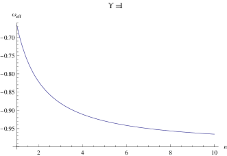
Figure 2: $w_{eff}|_{\Upsilon=1}$ vs $n$ for eq.(73).

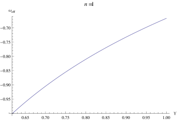
Figure 3: $w_{eff}|_{n=1}$ vs $\Upsilon$ for eq.(74).

In the case of the matter-dominated eras (radiation or the cold dark matter), it is sufficient to add the density of the matter $\rho_{M}$, to the right-hand side of eq.(49) and consider $H=1/kt$, where $k=2$ for the radiation-dominated era and $k=3/2$ for the cold dark matter-dominated era.
For the specific model (62), we obtain

$$3M_{P}^{2}H^{2}=\rho_{M}+\rho_{eff}\ ,$$ (76)

where

$$\rho_{eff}\equiv\frac{M^{4+2n}}{H^{2n}(18\Upsilon-6-6\Upsilon k)^{n}}\times(\text{left-hand side of eq.(\ref{cos14})})\ .$$ (77)

Note that in the matter-dominated era $\frac{\rho_{eff}}{\rho_{M}}\ll 1$, so that for $n=1$ we obtain

$$3M_{P}^{2}H^{2}=\rho_{M}+\Omega\frac{M^{6}}{H^{2}}\ ,$$ (78)

where [31]

$$\begin{split}&\Omega|_{\text{radiation-dominated era}}=\frac{1}{6}(\Upsilon^{2}-7\Upsilon-3)\ ,\\ &\Omega|_{\text{dark matter-dominated era}}=\frac{1}{4}(\Upsilon^{2}-3\Upsilon-2)\ .\end{split}$$ (79)

Thus, using eq.(78) and $\frac{\rho_{eff}}{\rho_{M}}\ll 1$, we have

$$3M_{P}^{2}H^{2}=\rho_{M}+3\Omega\frac{M_{P}^{2}M^{6}}{\rho_{M}}\ .$$ (80)

¿From eq.(78) or eq.(80), it follows that in the matter-dominated eras, $\rho_{eff}\rho_{M}\propto 1$. So, eventually $\rho_{eff}$ will be dominated and the mechanism for the power-law acceleration can occur.

5.2 $\Upsilon=0$ case

Let us now focus our attention on the special case $\Upsilon=0$. This special case was previously studied in [32] in a different from ours approach .

To begin with, we note that eq.(49) is valid for any $\Upsilon$. On the other hand, for $\Upsilon=0$ this equation reduces to an algebraic equation for the Hubble parameter. So, if the equation has a solution we find that it is the de Sitter solution which is suitable for the late-time cosmology.
For instance, consider (62) for $n=1$ and $\Upsilon=0$. Then equation (49) with the matter density on the right-hand side yields

$$3M_{P}^{2}H^{2}=\rho_{M}+\frac{1}{6}\frac{M^{6}}{H^{2}}\ .$$ (81)

This equation is similar to eq.(78), but note that the equation (81) is valid during all the cosmological eras. Solving this equation for $H^{2}$, we find

$$6M_{P}^{2}H^{2}=\rho_{M}+\sqrt{\rho_{M}^{2}+2M_{P}^{2}M^{6}}.$$ (82)

So, at the late-time we have

$$3H^{2}\rightarrow\sqrt{\frac{1}{2}}\frac{M^{3}}{M_{P}}\ .$$ (83)

6 Discussion

Let us outline the main results of the paper. We have analyzed the recently proposed version of $f(R)$ gravity with broken four-dimensional diffeomorphism by changing the constant in front of the total divergence term that arises in the ($3+1$)-decomposition of scalar curvature. We have shown that this naive modification of theory is not consistent from the Hamiltonian point of view due to the fact that the Hamiltonian constraint is a second-class constraint with itself. We have proposed two ways how to resolve this issue. The first one is based on the observation that the Poisson bracket between the Hamiltonian constraint vanishes when we impose an additional constraint on the scalar field $B$. However, a careful Hamiltonian analysis shows that the restricted $f(R)$ gravity with this additional constraint is equivalent to the ordinary Einstein-Hilbert action. Further, we have argued that the right way how to correctly define the restricted $f(R)$ theory of gravity is to include the terms which are invariant under the spatial diffeomorphism , for example, the gradient of the lapse. We have performed the Hamiltonian analysis of this theory and we have found that it is consistent one from the Hamiltonian point of view and have shown that this theory is equivalent to the low-energy limit of non-projectable $f(R)$ HL gravity. Moreover, we have identified two global first-class constraints, which ensure that the Hamiltonian is invariant under the global time reparametrization and global rescaling of lapse. Finally, we have discussed some cosmological application of the restricted $f(R)$ gravity and have found several interesting implications. In particular, we have discussed the differences between the usual $R^{n}$ gravity, with $n<0$ and its corresponding restricted version. In addition, it has been shown how the asymptotic solutions of $R^{n}$ gravity can be changed by the broken symmetry. Moreover, we have found that it is possible to find the de Sitter solution in the case of $R^{2}$ gravity, which does not exist in the case of $\Upsilon=1$. It has been also found that with a suitable choice of the parameter $\Upsilon$, this solution describes the inflation phase of cosmology with the correct number of e-foldings. These results imply nice physical meaning of the parameter $\Upsilon$: For the early Universe $\Upsilon$ determines the scale of inflation and the stability of de Sitter solution (see eq.(65)), while for the late-time cosmology, $\Upsilon$ determines the parameter in the equation of state, which can be measured (see eq.(71) and discussion after it).

The results presented are encouraging and the cosmological applications in the context of restricted $f(R)$ gravity certainly desrve to be studied further and in more details. Specifically, one should analyze the fluctuations around the cosmological solutions in this theory. We expect that there is an additional scalar mode and its behaviour should be analyzed. It would also be interesting to analyze this mode around the flat background following the corresponding analysis in the case of the healthy extension of non-projectable HL gravity [9]. We hope to return to this problem in future.

Acknowledgements
The work of J.K. was supported by the Grant Agency of the Czech Republic under the grant P201/12/G028.

References

- [1] P. A. R. Ade et al. [Planck Collaboration], “Planck 2015 results. XX. Constraints on inflation,” arXiv:1502.02114 [astro-ph.CO].
- [2] A. De Felice and S. Tsujikawa, “f(R) theories,” Living Rev. Rel. 13 (2010) 3 [arXiv:1002.4928 [gr-qc]].
- [3] P. Horava, “Quantum Gravity at a Lifshitz Point,” Phys. Rev. D 79 (2009) 084008 [arXiv:0901.3775 [hep-th]].
- [4] P. Horava, “Membranes at Quantum Criticality,” JHEP 0903 (2009) 020 [arXiv:0812.4287 [hep-th]].
- [5] P. Horava, “Quantum Criticality and Yang-Mills Gauge Theory,” arXiv:0811.2217 [hep-th].
- [6] M. Li and Y. Pang, “A Trouble with Hořava-Lifshitz Gravity,” JHEP 0908 (2009) 015 [arXiv:0905.2751 [hep-th]].
- [7] M. Henneaux, A. Kleinschmidt and G. L. Gomez, “A dynamical inconsistency of Horava gravity,” arXiv:0912.0399 [hep-th].
- [8] D. Blas, O. Pujolas and S. Sibiryakov, “Consistent Extension of Horava Gravity,” Phys. Rev. Lett. 104 (2010) 181302 [arXiv:0909.3525 [hep-th]].
- [9] D. Blas, O. Pujolas and S. Sibiryakov, “Models of non-relativistic quantum gravity: The Good, the bad and the healthy,” JHEP 1104 (2011) 018 [arXiv:1007.3503 [hep-th]].
- [10] D. Blas, O. Pujolas and S. Sibiryakov, “Comment on ‘Strong coupling in extended Horava-Lifshitz gravity’,” Phys. Lett. B 688 (2010) 350 [arXiv:0912.0550 [hep-th]].
- [11] J. Kluson, “Note About Hamiltonian Formalism of Healthy Extended Horava-Lifshitz Gravity,” JHEP 1007 (2010) 038 [arXiv:1004.3428 [hep-th]].
- [12] W. Donnelly and T. Jacobson, “Hamiltonian structure of Horava gravity,” Phys. Rev. D 84 (2011) 104019 [arXiv:1106.2131 [hep-th]].
- [13] S. Mukohyama, R. Namba, R. Saitou and Y. Watanabe, “Hamiltonian analysis of nonprojectable Ho ava-Lifshitz gravity with symmetry,” Phys. Rev. D 92 (2015) 2, 024005 [arXiv:1504.07357 [hep-th]].
- [14] M. Chaichian, J. Kluson and M. Oksanen, “Non-Projectable Horava-Lifshitz Gravity without Unwanted Scalar Graviton,” arXiv:1509.06528 [gr-qc].
- [15] J. Kluson, “Horava-Lifshitz f(R) Gravity,” JHEP 0911 (2009) 078 [arXiv:0907.3566 [hep-th]].
- [16] J. Kluson, S. Nojiri, S. D. Odintsov and D. Saez-Gomez, “U(1) Invariant Horava-Lifshitz Gravity,” Eur. Phys. J. C 71 (2011) 1690 [arXiv:1012.0473 [hep-th]].
- [17] J. Kluson, “Note About Hamiltonian Formalism of Modified Hořava-Lifshitz Gravities and Their Healthy Extension,” Phys. Rev. D 82 (2010) 044004 [arXiv:1002.4859 [hep-th]].
- [18] J. Kluson, “New Models of f(R) Theories of Gravity,” Phys. Rev. D 81 (2010) 064028 [arXiv:0910.5852 [hep-th]].
- [19] S. Carloni, M. Chaichian, S. Nojiri, S. D. Odintsov, M. Oksanen and A. Tureanu, “Modified first-order Horava-Lifshitz gravity: Hamiltonian analysis of the general theory and accelerating FRW cosmology in power-law F(R) model,” Phys. Rev. D 82 (2010) 065020 [Phys. Rev. D 85 (2012) 129904] [arXiv:1003.3925 [hep-th]].
- [20] M. Chaichian, S. Nojiri, S. D. Odintsov, M. Oksanen and A. Tureanu, “Modified F(R) Horava-Lifshitz gravity: a way to accelerating FRW cosmology,” Class. Quant. Grav. 27 (2010) 185021 [Class. Quant. Grav. 29 (2012) 159501] [arXiv:1001.4102 [hep-th]].
- [21] M. Chaichian, M. Oksanen and A. Tureanu, “Hamiltonian analysis of non-projectable modified F(R) Horava-Lifshitz gravity,” Phys. Lett. B 693 (2010) 404 [Phys. Lett. B 713 (2012) 514] [arXiv:1006.3235 [hep-th]].
- [22] A. Ghalee, “Notes on diffeomorphisms symmetry of f(R)gravity in the cosmo- logical context,” Eur. Phys. J. C 76, (2016), 136 [arXiv:1510.05353 [gr-qc]].
- [23] E. Gourgoulhon, “3+1 Formalism and Bases of Numerical Relativity,” arXiv:gr-qc/0703035.
- [24] K. V. Kuchar, “Does an unspecified cosmological constant solve the problem of time in quantum gravity?,” Phys. Rev. D 43 (1991) 3332. doi:10.1103/PhysRevD.43.3332
- [25] J. D. Barrow and A. C. Ottewill, “The stability of general relativistic cosmological theory,” J. Phys. A 16, 2757 (1983); J. C. de Souza and V. Faraoni, “The phase-space view of gravity,” Classical Quantum Gravity 24, 3637 (2007).
- [26] A . A. Starobinsky, “A new type of isotropic cosmological models without singularity,” Phys. Lett. B. 91, (1980) 99.
- [27] S. Weinberg, “Asymptotically Safe Inflation,” Phys. Rev. D. 81, 083535, (2010).
- [28] S. M. Carroll, V. Duvvuri, M. Trodden, and M. S. Turner,“Is cosmic speed-up due to new gravitational physics?,” Phys. Rev. D 70 043528 (2004).
- [29] In Ref. [28], the authors study by using the so-called the Einstein-frame. Here, we do not use this frame. For example from eq. (68) to eq. (69), we use an approximation. To find what is the meaning of the similar approximation when we take in the Einstein-frame, see discussion of Ref. [28] that the authors argued that ”..Soon thereafter, the potential is well-approximated by…”.
- [30] L. Amendola, D. Polarski, S. Tsujikawa,“Are f(R) Dark Energy Models Cosmologically Viable?,” Phys. Rev. Lett. 98, 131302, (2007). Note that the authors of this paper considered the usual gravity with the matters. They showed that at the late-time, when the density of the matters are diluted by the expansion of the universe, in addition to eq. (73), it is possible that . Thus it is unclear that we have after the dark matter-dominated era in the such models. Note that for this case, in this reference, as we have .
- [31] To find in eq. (79), we have a factor as . For this reason, we cannot obtain this term if we take . Actually, has this problem in the radiation-dominated ere, because in this era . One can regard this note as an advantage of our model.
- [32] C. Gao, “Modified gravity in Arnowitt-Deser-Misner formalism,” Phys. Lett. B 684, 85, (2010).
- [33] G. W. Gibbons and S. W. Hawking, “Action Integrals and Partition Functions in Quantum Gravity,” Phys. Rev. D 15 (1977) 2752. doi:10.1103/PhysRevD.15.2752
- [34] A. Guarnizo, L. Castaneda and J. M. Tejeiro, “Boundary Term in Metric f(R) Gravity: Field Equations in the Metric Formalism,” Gen. Rel. Grav. 42 (2010) 2713 doi:10.1007/s10714-010-1012-6 [arXiv:1002.0617 [gr-qc]].
- [35] E. Dyer and K. Hinterbichler, “Boundary Terms, Variational Principles and Higher Derivative Modified Gravity,” Phys. Rev. D 79 (2009) 024028 doi:10.1103/PhysRevD.79.024028 [arXiv:0809.4033 [gr-qc]].