Elastic, thermal expansion, plastic and rheological processes – theory and experiment

Abstract

Rocks are important examples for solid materials where, in various engineering situations, elastic, thermal expansion, rheological/viscoelastic and plastic phenomena each may play a remarkable role. Nonequilibrium continuum thermodynamics provides a consistent way to describe all these aspects in a unified framework. This we present here in a formulation where the kinematic quantities allow arbitrary nonzero initial (e.g., in situ) stresses and such initial configurations which – as a consequence of thermal or remanent stresses – do not satisfy the kinematic compatibility condition. The various characteristic effects accounted by the obtained theory are illustrated via experimental results where loaded solid samples undergo elastic, thermal expansion and plastic deformation and exhibit rheological behaviour. From the experimental data, the rheological coefficients are determined, and the measured temperature changes are also explained by the theory.

Dedicated to the memory of Zoltán Szarka (1927–2015).

Keywords

solids, elasticity, rheology, thermal expansion, plasticity, thermodynamics

1 Introduction

Motivated by problems in rock mechanics and similar challenges in the continuum theory of solids, in the last few years, our research object has been to achieve an amalgamation of a new approach [1, 2, 3, 4] to the problem of objectivity and of material frame indifference – based on Matolcsi’s framework [5, 6, 7, 8] – with a recent activity in nonequilibrium thermodynamics [9, 10, 11, 12] that focuses on the role of thermodynamical stability and on a constructive quantitative exploitation of the content of the second law of thermodynamics. Here, we present how this program has accomplished a theoretical framework for the continuum thermo-elasto-visco-plasto-mechanics of solids.

Accordingly, the aspects covered currently are:

• elasticity, an immediate response to mechanical loading, and during which mechanical energy is conserved;

• rheology, which, in contrast, is a delayed response, with mechanical energy partially dissipated, and which may be attributed to viscous damping, for instance;

• plasticity, which is permanent shape change caused by mechanical loading: a change of the unloaded shape;

• thermal expansion, and the thermal stress generated by it;

• and heat conduction.

In parallel to the general level – large deformation theory, general constitutive equations –, we consider it inevitable to exhibit (and countercheck!) the applicability of the formulation to practical concrete examples. To this end, we have performed experiments on which the theory can be applied and tested. The experimental results presented here illustrate the various predictions of the theory both qualitatively and quantitatively. Via this simple yet widely informative and insightful experimental example – mechanical and thermal monitoring of uniaxial stretching of polyamide-6 plastic samples –, the various thermomechanical effects in solids are well demonstrated and the correspondence to the theoretical expectations are satisfactorily established.

Therefore, though the theoretical framework described here is capable to describe completely general situations, here our aim is to focus on the connection between theory and experiment so, at each component of our theoretical formulation, we take the simplest applicable concrete choice: small deformations, Hooke elasticity with constant elastic coefficients, constant specific heat, thermal expansion and heat conduction coefficients, and constant plastic change rate coefficient and yield stress. These assumptions satisfactorily suit the obtained experimental data.

We start the discussion with the kinematic quantities according to the mentioned recent objective approach. Then we build elasticity, thermal expansion and plasticity around these quantities, via continuum thermodynamics. We show how the predicted behaviours can be observed experimentally. Next, we incorporate rheology into the theory, and point out how the example measurement results indicate the presence of rheology both on the mechanical and the thermal side. We determine the rheological coefficients from the experimental data, and discuss the related arising numerical challenges and the used solutions that enabled us to obtain these coefficients reliably. In the Discussion section, we summarize the most important outcomes and lessons, and outline the future perspectives and aims. Technical details concerning the measurement can be found in the Appendix.

2 The kinematic ingredients

We start with a succint account of the objectivity respecting definition of the involved kinematic quantities, presented in detail in [1, 2, 3, 4]. For continua – solids, liquids and gases each – the motion determines the instantaneous distance of any two material points. This defines an instantaneous metric $\hbox{$\mathbf{h}$}\kern-5.05559pt\widetilde{\hbox to4.5556pt{\vphantom{$\mathbf{h}$}}}\kern 0.49997pt$ on the material manifold. Hereafter, overtilde indicates tensors on the material manifold, operating on the material tangent vectors. For solids, the novel and important notion is the relaxed or self-metric $\hbox{$\mathbf{g}$}\kern-4.55002pt\widetilde{\hbox to4.10004pt{\vphantom{$\mathbf{g}$}}}\kern 0.44998pt$, which describes the distances of material points when the solid is in an unstressed, relaxed state. In such a state, $\hbox{$\mathbf{h}$}\kern-5.05559pt\widetilde{\hbox to4.5556pt{\vphantom{$\mathbf{h}$}}}\kern 0.49997pt=\hbox{$\mathbf{g}$}\kern-4.55002pt\widetilde{\hbox to4.10004pt{\vphantom{$\mathbf{g}$}}}\kern 0.44998pt$. The relaxed metric characterizes the relaxed shape of a solid body.

For the purposes of the elastic state variable, the appropriate kinematic quantity can be defined from

$$\hbox{$\mathbf{A}$}\kern-6.82503pt\widetilde{\hbox to6.15005pt{\vphantom{$\mathbf{A}$}}}\kern 0.67497pt=\hbox{$\mathbf{g}$}\kern-4.55002pt\widetilde{\hbox to4.10004pt{\vphantom{$\mathbf{g}$}}}\kern 0.44998pt^{-1}\hbox{$\mathbf{h}$}\kern-5.05559pt\widetilde{\hbox to4.5556pt{\vphantom{$\mathbf{h}$}}}\kern 0.49997pt,$$ (1)

the elastic shape symmetric tensor – the (objective generalization of the) right Cauchy–Green tensor –, as

$$\hbox{$\mathbf{D}$}\kern-6.95142pt\widetilde{\hbox to6.26395pt{\vphantom{$\mathbf{D}$}}}\kern 0.68747pt=\frac{1}{2}\ln\hbox{$\mathbf{A}$}\kern-6.82503pt\widetilde{\hbox to6.15005pt{\vphantom{$\mathbf{A}$}}}\kern 0.67497pt.$$ (2)

This elastic deformedness tensor $\hbox{$\mathbf{D}$}\kern-6.95142pt\widetilde{\hbox to6.26395pt{\vphantom{$\mathbf{D}$}}}\kern 0.68747pt$ is on which elastic stress, $\hbox{$\mathchoice{\hbox{\boldmath{$\sigma$}}}{\hbox{\boldmath{$\sigma$}}}{\hbox{\boldmath{$\scriptstyle\sigma$}}}{\hbox{\boldmath{$\scriptscriptstyle\sigma$}}}$}\kern-16.63959pt\widetilde{\hbox to14.99399pt{\vphantom{$\mathchoice{\hbox{\boldmath{$\sigma$}}}{\hbox{\boldmath{$\sigma$}}}{\hbox{\boldmath{$\scriptstyle\sigma$}}}{\hbox{\boldmath{$\scriptscriptstyle\sigma$}}}$}}}\kern 1.6456pt$, is considered to depend on, linearly (Hooke’s law) or nonlinearly (e.g., a neo-Hooke model). This logarithmic type – objectively generalized Hencky strain – definition (2) is distinguished both geometrically (the spherical/trace part of describes the volumetric change and the deviatoric part corresponds to the constant-volume changes, even for large deformations [1, 13, 14]) and experimentally (for example, large-deformation stress in materials like hard rubber is most linear in this logarithmic tensor [15, 16], the five-parameter Murnaghan model of nonlinear elasticity also performs the best in this logarithmic variable [17], and see also [18].

Via the (objective generalization of the) deformation gradient, the material tangent vectors can be mapped to the spatial vectors. Our material tensors ($\hbox{$\mathbf{h}$}\kern-5.05559pt\widetilde{\hbox to4.5556pt{\vphantom{$\mathbf{h}$}}}\kern 0.49997pt$, $\hbox{$\mathbf{A}$}\kern-6.82503pt\widetilde{\hbox to6.15005pt{\vphantom{$\mathbf{A}$}}}\kern 0.67497pt$ etc.) are correspondingly mapped to their spatial counterpart ($\mathbf{h}$, $\mathbf{A}$ etc.). The change of $\hbox{$\mathbf{h}$}\kern-5.05559pt\widetilde{\hbox to4.5556pt{\vphantom{$\mathbf{h}$}}}\kern 0.49997pt$ in time, and thus the time derivative of $\mathbf{A}$, can be calculated with the aid of the velocity gradient

$$\mathbf{L}=\mathbf{v}\otimes{\overset{{\scriptscriptstyle\leftarrow}}{\nabla}}$$ (3)

(and its transpose $\mathbf{L}^{\text{transp}}={\overset{{\scriptscriptstyle\rightarrow}}{\nabla}}\otimes\mathbf{v}$), and one finds

$$\dot{\mathbf{A}}=\mathbf{L}\mathbf{A}+\mathbf{A}\mathbf{L}^{\text{transp}}$$ (4)

for the comoving time derivative $\dot{\mathbf{A}}$, as long as only elasticity is involved ($\hbox{$\mathbf{g}$}\kern-4.55002pt\widetilde{\hbox to4.10004pt{\vphantom{$\mathbf{g}$}}}\kern 0.44998pt=\text{const.}$).

Thermal expansion is the phenomenon that the unstressed and relaxed size, hence, the relaxed metric, of solid bodies depends on temperature: $\hbox{$\mathbf{g}$}\kern-4.55002pt\widetilde{\hbox to4.10004pt{\vphantom{$\mathbf{g}$}}}\kern 0.44998pt=\hbox{$\mathbf{g}$}\kern-4.55002pt\widetilde{\hbox to4.10004pt{\vphantom{$\mathbf{g}$}}}\kern 0.44998pt(T)$($T$ denoting absolute temperature throughout this paper). If the material is isotropic, which we assume in what follows, then this temperature dependence is a simple scalar rescaling:

$$\hbox{$\mathbf{g}$}\kern-4.55002pt\widetilde{\hbox to4.10004pt{\vphantom{$\mathbf{g}$}}}\kern 0.44998pt{(T_{2})} =\Lambda{(T_{1},T_{2})}^{2}\hbox{$\mathbf{g}$}\kern-4.55002pt\widetilde{\hbox to4.10004pt{\vphantom{$\mathbf{g}$}}}\kern 0.44998pt{(T_{1})},$$ (5)

$$\alpha(T) =\lim\limits_{\Delta T\to 0}\frac{\Lambda\left(T,T+\Delta T\right)-1}{\Delta T},$$ (6)

the latter formula defining the linear thermal expansion coefficient $\alpha$. It follows that, when temperature changes in time at a material point, we have

$$\dot{\hbox{$\mathbf{g}$}\kern-4.55002pt\widetilde{\hbox to4.10004pt{\vphantom{$\mathbf{g}$}}}\kern 0.44998pt}=\left(\frac{\mathrm{d}}{\mathrm{d}T}\hbox{$\mathbf{g}$}\kern-4.55002pt\widetilde{\hbox to4.10004pt{\vphantom{$\mathbf{g}$}}}\kern 0.44998pt\right)\dot{T}=2\alpha(T)\dot{T}\,\hbox{$\mathbf{g}$}\kern-4.55002pt\widetilde{\hbox to4.10004pt{\vphantom{$\mathbf{g}$}}}\kern 0.44998pt$$ (7)

for the comoving time derivative of the relaxed metric, and (4) is generalized to

$$\dot{\mathbf{A}}=\mathbf{L}\mathbf{A}+\mathbf{A}\mathbf{L}^{\text{transp}}-2\alpha\dot{T}\mathbf{A}.$$ (8)

Plasticity (see, e.g., the recent monography [19]) is, in our language, another phenomenon involving the change of $\hbox{$\mathbf{g}$}\kern-4.55002pt\widetilde{\hbox to4.10004pt{\vphantom{$\mathbf{g}$}}}\kern 0.44998pt$: strong enough mechanical stress causes the relaxed shape – and metric – of a solid to change permanently. This change can be characterized by the plastic change rate tensor

$$\hbox{$\mathbf{Z}$}\kern-5.56113pt\widetilde{\hbox to5.01115pt{\vphantom{$\mathbf{Z}$}}}\kern 0.54997pt=\frac{1}{2}\hbox{$\mathbf{g}$}\kern-4.55002pt\widetilde{\hbox to4.10004pt{\vphantom{$\mathbf{g}$}}}\kern 0.44998pt^{-1}\dot{\hbox{$\mathbf{g}$}\kern-4.55002pt\widetilde{\hbox to4.10004pt{\vphantom{$\mathbf{g}$}}}\kern 0.44998pt}_{\text{plastic}},$$ (9)

with which the total kinematic time evolution equation is

$$\dot{\mathbf{A}}=\mathbf{L}\mathbf{A}+\mathbf{A}\mathbf{L}^{\text{transp}}-2\alpha\dot{T}\mathbf{A}-2\mathbf{Z}\mathbf{A}.$$ (10)

In the subsequent sections, we restrict ourselves to the small-deformation regime, $\lVert{\mathbf{D}}\rVert\ll 1$, $\mathbf{A}=\mathrm{e}^{2\mathbf{D}}\approx\mathbf{1}+2\mathbf{D}$, where (10) leads, in the leading order of $\mathbf{D}$, to $2\dot{\mathbf{D}}=\mathbf{L}+\mathbf{L}^{\text{transp}}-2\alpha\dot{T}\mathbf{1}-2\mathbf{Z}$, rearrangable as

$$\mathbf{L}^{\text{sym}}=\dot{\mathbf{D}}+\alpha\dot{T}\mathbf{1}+\mathbf{Z}$$ (11)

(${}^{\text{sym}}$ standing for symmetric part). Further, for our purposes below, the thermal expansion coefficient can be taken as constant.

3 Comparison with the usual approach to kinematic quantities

Conventionally, a reference frame and an initial time $t_{0}$ is chosen, and displacements are considered in the space of this reference frame and are measured related to positions at $t_{0}$. From the displacements, the deformation gradient is defined, and the various strain measures are constructed from the deformation gradient. One consequence of this approach is that initial strains are necessarily zero, and the corresponding elastic stress is also zero. Initial strains also necessarily satisfy the compatibility condition.

Furthermore, when thermal expansion is also considered then a homogeneous initial temperature distribution is assumed as well.

One of our aims with the alternative kinematic formulation expounded in the preceding section was to generalize this approach to situations where initial (e.g., in situ) stresses are unavoidably nonzero, the initial temperature distribution is far from homogeneous, or where in situ or remanent stresses indicate that the compatibility condition is violated already initially. Namely, as we have shown [1, 2, 3, 4], while the instantaneous metric $\hbox{$\mathbf{h}$}\kern-5.05559pt\widetilde{\hbox to4.5556pt{\vphantom{$\mathbf{h}$}}}\kern 0.49997pt$ is a flat Riemann metric by definition, the relaxed Riemann metric $\hbox{$\mathbf{g}$}\kern-4.55002pt\widetilde{\hbox to4.10004pt{\vphantom{$\mathbf{g}$}}}\kern 0.44998pt$ is not necessarily flat (so the compatibility condition – see its finite deformation version lengthy formula in [1, 2] – is violated), for example as a consequence of some plastic preceding history or an inhomogeneous temperature distribution. Then these two metrics necessarily differ at some parts of the material, causing there nonzero elastic deformedness, and thus leading to nonzero elastic stress (remanent, ”frozen” stress).

In our generalized formulation, strains – which are nevertheless important notions for experimental purposes – can be given as time integrals of the various terms of (11) from reference time to current time: total strain $\varepsilon$ is the time integral of the lhs term, elastic strain $\mathchoice{\hbox{\boldmath{$\varepsilon$}}}{\hbox{\boldmath{$\varepsilon$}}}{\hbox{\boldmath{$\scriptstyle\varepsilon$}}}{\hbox{\boldmath{$\scriptscriptstyle\varepsilon$}}}_{\text{el}}$ is that of the first term on the rhs, thermal expansion strain $\mathchoice{\hbox{\boldmath{$\varepsilon$}}}{\hbox{\boldmath{$\varepsilon$}}}{\hbox{\boldmath{$\scriptstyle\varepsilon$}}}{\hbox{\boldmath{$\scriptscriptstyle\varepsilon$}}}_{\text{th}}$ is that of the second one, and plastic strain $\mathchoice{\hbox{\boldmath{$\varepsilon$}}}{\hbox{\boldmath{$\varepsilon$}}}{\hbox{\boldmath{$\scriptstyle\varepsilon$}}}{\hbox{\boldmath{$\scriptscriptstyle\varepsilon$}}}_{\text{pl}}$ is the integral of the third term. In the small deformation regime involved in the experiments below, these definitions suffice and no finite deformation complication needs to be addressed.

4 Mechanics and thermodynamics

Our chosen elastic constitutive equation is Hooke’s law:

$$\mathchoice{\hbox{\boldmath{$\sigma$}}}{\hbox{\boldmath{$\sigma$}}}{\hbox{\boldmath{$\scriptstyle\sigma$}}}{\hbox{\boldmath{$\scriptscriptstyle\sigma$}}}=E^{\text{dev}}\mathbf{D}^{\text{dev}}+E^{\text{sph}}\mathbf{D}^{\text{sph}}$$ (12)

with the spherical and deviatoric components and elastic coefficients

$$\mathbf{D}^{\text{sph}} ={\textstyle\frac{1}{3}}(\;\!{\text{tr}}\;\!\mathbf{D})\mathbf{1}, \mathbf{D}^{\text{dev}} =\mathbf{D}-\mathbf{D}^{\text{sph}},$$ (13)

$$E^{\text{sph}} =3K, E^{\text{dev}} =2G.$$ (14)

For us here, it suffices to consider $E^{\text{dev}}$ and $E^{\text{sph}}$ as constant. From (12), it is easy to show [2] that the classic Duhamel–Neumann formula for thermoelasticity [20] is recovered as a special case, via transforming from the elastic deformedness variable to the total strain and imposing that, at the initial reference time,

• elastic deformedness is zero,

• the temperature distribution is homogeneous,

• and plastic change does not occur.

The first law of continuum thermodynamics, i.e., the balance of internal energy, reads

$$\varrho\dot{e}=-\mathbf{j}_{e}\cdot{\overset{{\scriptscriptstyle\leftarrow}}{\nabla}}+\;\!{\text{tr}}\;\!\left(\mathchoice{\hbox{\boldmath{$\sigma$}}}{\hbox{\boldmath{$\sigma$}}}{\hbox{\boldmath{$\scriptstyle\sigma$}}}{\hbox{\boldmath{$\scriptscriptstyle\sigma$}}}\mathbf{L}^{\text{sym}}\right)$$ (15)

for the specific internal energy $e(\mathbf{D},T)$ and its current $\mathbf{j}_{e}$, both to be specified constitutively (and the mass density $\varrho$ being constant in the small deformation regime). Similarly, the balance for specific entropy $s(\mathbf{D},T)$ is

$$\varrho\dot{s}={-\mathbf{j}_{s}\cdot{\overset{{\scriptscriptstyle\leftarrow}}{\nabla}}+\pi_{s}},$$ (16)

where we take the simplest and standard choice $\mathbf{j}_{s}=\mathbf{j}_{e}/T$ for the the entropy current $\mathbf{j}_{s}$, $s$ must be thermodynamically consistent with $e$ (i.e., the Gibbs relation must hold between them), and entropy production must be positive definite, $\pi_{s}\geq 0$. Specifically, we take

$$\mathbf{j}_{e}=\lambda{\overset{{\scriptscriptstyle\rightarrow}}{\nabla}}\frac{1}{T},$$ (17)

that is, standard Fourier heat conduction, with positive coefficient $\lambda$, and

$$e =cT+\left\{\frac{E^{\text{dev}}}{2\varrho}\;\!{\text{tr}}\;\!\mathopen{}\mathclose{{}\left[{\left(\mathbf{D}^{\text{dev}}\right)^{2}}}\right]+\frac{E^{\text{sph}}}{2\varrho}\;\!{\text{tr}}\;\!\mathopen{}\mathclose{{}\left[{\left(\mathbf{D}^{\text{sph}}\right)^{2}}}\right]\right\}$$

$$\quad+\frac{E^{\text{sph}}}{\varrho}T\alpha\;\!{\text{tr}}\;\!\mathbf{D}^{\text{sph}},$$ (18)

for specific internal energy, in which the first term provides the constant specific heat $c$, the middle term describes elastic energy, and the last one is responsible for thermal expansion. The corresponding specific entropy is determined up to an additive constant, as

$$s=c\ln\frac{T}{T_{*}}+\frac{E^{\text{sph}}}{\varrho}\alpha\;\!{\text{tr}}\;\!\mathbf{D}^{\text{sph}}$$ (19)

with an arbitrarily auxiliary constant $T_{*}$. In the resulting entropy production,

$$\pi_{s} ={\overset{{\scriptscriptstyle\rightarrow}}{\nabla}}\frac{1}{T}\cdot\mathbf{j}_{e}+\frac{1}{T}\;\!{\text{tr}}\;\!\mathopen{}\mathclose{{}\left(\mathchoice{\hbox{\boldmath{$\sigma$}}}{\hbox{\boldmath{$\sigma$}}}{\hbox{\boldmath{$\scriptstyle\sigma$}}}{\hbox{\boldmath{$\scriptscriptstyle\sigma$}}}\mathbf{Z}}\right)$$ (20)

$$={\overset{{\scriptscriptstyle\rightarrow}}{\nabla}}\frac{1}{T}\cdot\mathbf{j}_{e}+\frac{E^{\text{dev}}}{T}\;\!{\text{tr}}\;\!(\mathbf{D}^{\text{dev}}\mathbf{Z})+\frac{E^{\text{sph}}}{T}\;\!{\text{tr}}\;\!(\mathbf{D}^{\text{sph}}\mathbf{Z}).$$

the first term of the rhs is non-negative due to (17), and we ensure the two further terms to be positive definite by choosing the plastic constitutive equation as

$$\mathbf{Z}=\Gamma\dot{\mathbf{D}}^{\text{dev}}$$ (21)

with

$$\Gamma =\gamma H\mathopen{}\mathclose{{}\left(\;\!{\text{tr}}\;\!\mathopen{}\mathclose{{}\left[{\left(\mathbf{D}^{\text{dev}}\right)^{2}}}\right]-\frac{2}{3}D_{\text{crit}}^{2}}\right)$$

$$\quad\times H\mathopen{}\mathclose{{}\left(\;\!{\text{tr}}\;\!\mathopen{}\mathclose{{}\left[{\left(\mathbf{D}^{\text{dev}}\dot{\mathbf{D}}^{\text{dev}}\right)}}\right]}\right),$$ (22)

where $\gamma$ and $D_{\text{crit}}$ are positive constants, and $H$ is the Heaviside function.

Equation (21) describes a natural plasticity theory:

• the plastic change rate is proportional to the deviatoric elastic change rate,

• the yield criterion is the von Mises one (note that, now, stress is in a Hookean relationship with elastic deformedness so $\mathbf{D}$ can be replaced by $\sigma$, and $D_{\text{crit}}$ is equivalent to a $\sigma_{\text{crit}}$, the von Mises yield stress),

• and plastic change is switched off during unloading, as a consequence of the second Heaviside factor that ensures the thermodynamical requirement $\pi_{s}\geq 0$.

For temperature dependent coefficients $E^{\text{sph}}$, $E^{\text{dev}}$, $\alpha$, $c$, for more general internal energy, for large deformations, and for anisotropic materials, one can derive similar though somewhat more complicated formulae.

The change of temperature is determined by the rate equation derivable from (18) with (15), (12) and (11) substituted:

$$\varrho c\dot{T}=-\mathbf{j}_{e}\cdot{\overset{{\scriptscriptstyle\leftarrow}}{\nabla}}-E^{\text{sph}}\alpha T\;\!{\text{tr}}\;\!\dot{\mathbf{D}}^{\text{sph}}+E^{\text{dev}}\;\!{\text{tr}}\;\!(\mathbf{D}^{\text{dev}}\mathbf{Z}).$$ (23)

The first term here gives account of the effect of heat. The second term is the source of the Joule–Thomson effect for solids: cooling during stretching and warming during compression. This is a reversible type change, a less obvious but inevitable manifestation of thermal expansion. The third term, on the contrary, describes an irreversible effect, being non-negative – as a result of the non-negativity of entropy production – and thus always causing warming whenever plastic change takes place.

Adding the mechanical equation of motion,

$$\varrho\dot{\mathbf{v}}=\mathchoice{\hbox{\boldmath{$\sigma$}}}{\hbox{\boldmath{$\sigma$}}}{\hbox{\boldmath{$\scriptstyle\sigma$}}}{\hbox{\boldmath{$\scriptscriptstyle\sigma$}}}\cdot{\overset{{\scriptscriptstyle\leftarrow}}{\nabla}},$$ (24)

or its force-equilibrial approximation (applied in what follows)

$$\mathchoice{\hbox{\boldmath{$\sigma$}}}{\hbox{\boldmath{$\sigma$}}}{\hbox{\boldmath{$\scriptstyle\sigma$}}}{\hbox{\boldmath{$\scriptscriptstyle\sigma$}}}\cdot{\overset{{\scriptscriptstyle\leftarrow}}{\nabla}}=\mathbf{0},$$ (25)

to the balance and constitutive equations above, we arrive at a closed set of dynamical equations: (3), (11)–(12), (17), (21)–(23) and (24) [or (25)]. (Volumetric forces can, naturally, be added if necessary.) Therefore, we can calculate any concrete process, provided the required amount of initial and boundary conditions are at hand.

5 Uniaxial processes – formulae and experimental illustration

We demonstrate the application of the obtained theoretical framework on uniaxial processes. Such situations are seminal because of two reasons: they are simple to calculate, and are capable to describe many experimental tests. For bodies with such special geometry, and assuming adiabaticity as well as symmetry respecting space independent boundary conditions, all quantities have a homogeneous distribution. In other words, quantities are time dependent but space independent. In appropriate coordinate system, tensors have at most only longitudinal ($||$) and transversal ($\perp$) components:

$$\sigma =\mathopen{}\mathclose{{}\left(\begin{smallmatrix}\sigma^{\rule{0.14699pt}{1.89871pt}\kern 0.29398pt\rule{0.14699pt}{1.89871pt}}&&\\ &\vphantom{|^{|}}\hphantom{|}0\hphantom{|}&\\ &&\vphantom{|^{|}}\hphantom{|}0\hphantom{|}\end{smallmatrix}}\right), \mathbf{D} =\mathopen{}\mathclose{{}\left(\begin{smallmatrix}D^{\rule{0.14699pt}{1.89871pt}\kern 0.29398pt\rule{0.14699pt}{1.89871pt}}&&\\ &D^{\hbox{\large$\scriptscriptstyle\perp$}}&\\ &&D^{\hbox{\large$\scriptscriptstyle\perp$}}\end{smallmatrix}}\right),$$

$$\varepsilon =\mathopen{}\mathclose{{}\left(\begin{smallmatrix}\varepsilon^{\rule{0.14699pt}{1.89871pt}\kern 0.29398pt\rule{0.14699pt}{1.89871pt}}&&\\ &\varepsilon^{\hbox{\large$\scriptscriptstyle\perp$}}&\\ &&\varepsilon^{\hbox{\large$\scriptscriptstyle\perp$}}\end{smallmatrix}}\right)$$ etc. (26)

The deviatoric and spherical parts read, consequently - shown on the example of $\mathbf{D}$:

$$\mathbf{D}^{\text{dev}} =\frac{1}{3}\mathopen{}\mathclose{{}\left(\begin{smallmatrix}2\mathopen{}\mathclose{{}\left(D^{\rule{0.14699pt}{1.89871pt}\kern 0.29398pt\rule{0.14699pt}{1.89871pt}}-D^{\hbox{\large$\scriptscriptstyle\perp$}}}\right)&&\\ &-\mathopen{}\mathclose{{}\left(D^{\rule{0.14699pt}{1.89871pt}\kern 0.29398pt\rule{0.14699pt}{1.89871pt}}-D^{\hbox{\large$\scriptscriptstyle\perp$}}}\right)&\\ &&-\mathopen{}\mathclose{{}\left(D^{\rule{0.14699pt}{1.89871pt}\kern 0.29398pt\rule{0.14699pt}{1.89871pt}}-D^{\hbox{\large$\scriptscriptstyle\perp$}}}\right)\end{smallmatrix}}\right),$$

$$\mathbf{D}^{\text{sph}} =\frac{1}{3}\mathopen{}\mathclose{{}\left(\begin{smallmatrix}D^{\rule{0.14699pt}{1.89871pt}\kern 0.29398pt\rule{0.14699pt}{1.89871pt}}+2D^{\hbox{\large$\scriptscriptstyle\perp$}}&&\\ &D^{\rule{0.14699pt}{1.89871pt}\kern 0.29398pt\rule{0.14699pt}{1.89871pt}}+2D^{\hbox{\large$\scriptscriptstyle\perp$}}&\\ &&D^{\rule{0.14699pt}{1.89871pt}\kern 0.29398pt\rule{0.14699pt}{1.89871pt}}+2D^{\hbox{\large$\scriptscriptstyle\perp$}}\end{smallmatrix}}\right).$$ (27)

Let us consider a mechanical equilibrial initial condition: $\mathbf{D}(t_{0})=\mathbf{0}$ at an initial time $t_{0}$ – when, naturally, no plastic change takes place: $\mathbf{Z}(t_{0})=\mathbf{0}$, and the purely elastic stress is zero –, and let $T_{0}$ denote the initial temperature. The total strain $\varepsilon$ – measured in experiments directly –, is, as mentioned earlier, the time integral of $\mathbf{L}^{\text{sym}}$ counted from $t_{0}$ so it also starts from zero at initial time. From a finite difference numerical perspective, the solution can be determined as follows. For definiteness, let us consider the case of force-driven process, where $\sigma^{\rule{0.20999pt}{2.71246pt}\kern 0.41998pt\rule{0.20999pt}{2.71246pt}}(t)$ is prescribed (taking into consideration that, in the small-deformation regime, the change of cross-section can be neglected). For strain-driven processes, a similar but somewhat more refined scheme is needed. Notably, the finite difference scheme outlined here is, despite its simplicity, suitable to demonstrate that the solution of the problem is well-defined. In addition, for many solid mechanical applications, its preciseness and performance may suffice with moderately small time steps.

So, assuming that all quantities are known up to time $t$, from the prescribed $\sigma^{\rule{0.20999pt}{2.71246pt}\kern 0.41998pt\rule{0.20999pt}{2.71246pt}}(t+\Delta t)$, which actually means the knowledge of $\mathchoice{\hbox{\boldmath{$\sigma$}}}{\hbox{\boldmath{$\sigma$}}}{\hbox{\boldmath{$\scriptstyle\sigma$}}}{\hbox{\boldmath{$\scriptscriptstyle\sigma$}}}(t+\Delta t)$, we determine $\mathbf{D}(t+\Delta t)$ via (12). Next, using $[\mathbf{D}(t+\Delta t)-\mathbf{D}(t)]/\Delta t$ as an approximation for $\dot{\mathbf{D}}$ during the interval $[t,t+\Delta t]$, we can apply (21) to calculate $\mathbf{Z}$ for this interval. Subsequently, (23) leads to a prediction of $\dot{T}$, which then offers $T(t+\Delta t)$. Also, it enables to determine $\mathbf{L}^{\text{sym}}=\dot{\mathchoice{\hbox{\boldmath{$\varepsilon$}}}{\hbox{\boldmath{$\varepsilon$}}}{\hbox{\boldmath{$\scriptstyle\varepsilon$}}}{\hbox{\boldmath{$\scriptscriptstyle\varepsilon$}}}}$ from (11) so, at last, we obtain $\mathchoice{\hbox{\boldmath{$\varepsilon$}}}{\hbox{\boldmath{$\varepsilon$}}}{\hbox{\boldmath{$\scriptstyle\varepsilon$}}}{\hbox{\boldmath{$\scriptscriptstyle\varepsilon$}}}(t+\Delta t)$ (which data is useful for comparison with experimentally measured values).

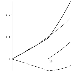
Figure 1: Characteristic time dependence of strains and temperature during uniaxial stretching by increasing force, according to the theory (arbitrary units, semi-quantitative plot: The thermal expansion coefficient is set unrealistically high to make its contribution visible). Temperature (dash-dotted line) first decreases – like for an adiabatically expanding gas – and then increases – due to plastic dissipation –, elastic strain (dotted line) increases as it follows the increased stress, and plastic strain (dashed line) appears only above the critical stress, causing that the total strain (solid line) starts to increase faster.

If a sample starts from the considered initial conditions, i.e., a relaxed and equilibrial state, and undergoes stretching with increasing force, the obtained theory predicts the following qualitative behaviour (see Fig. 1). Below the yield threshold, the Joule–Thomson effect is observable, and decreasing temperature results in some thermal contraction, which acts against the increase of elastic deformedness (but the latter dominates). When plastic change enters, it adds to the total strain increase, and the corresponding dissipation is a temperature increasing effect.

These phases can nicely be demonstrated experimentally when one monitors the temperature aspect during the stretching process. Here, we show five snapshots taken by a thermal camera during an example experiment performed on a polyamide-6 plastic sample (see Fig. 2), which depict the important stages (see Fig. 3). The last stage, failure, is not modelled here theoretically but is a phenomenon also expected to be possible to incorporate in a thermodynamical formulation [9, 10]. Namely, failure is likely to be a loss of thermodynamical stability of the continuum.

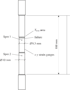
Figure 2: The outline of the experiment. The middle part of the sample was thinner, and was monitored by a thermal camera. Temperature values at the two displayed spots were numerically displayed (see Fig. 3), together with the maximal temperature in the rectangle area.

 

Figure 3: Snapshots taken by the thermal camera. The first one shows the initial state, then the quasi-adiabatic cooling is observable, then heat dissipation appears due to plastic change, then the plastic change reaches the whole thinner part of the sample, and finally failure occurs.

The same features can be observed in Fig. 4a, which presents the time series of loading force and temperature of a similar experiment performed on the same type of sample. Two loading–unloading cycles have been carried out, the second with larger maximal stress than the first, but both surely remained below the yield threshold. The third loading was not terminated, in order to enter the regime of plastic change and also to cause failure. Correspondingly, during the first two cycles, temperature first drops a bit and then it returns. The third loading also starts with cooling, until the plastic yield threshold is reached (see the small transient in the stress curve), and subsequently plastic dissipation starts to take the leading role, resulting in considerably raising temperature. According to (23) with (21) [and (28) below], the cooling part is linear in loading and the warming part is quadratic/parabolic.

(a)  (b)

Figure 4: (a) Measured temperature (grey line) and force (black line) as a function of time, during two complete loading–unloading uniaxial (strain-driven) stretching cycles followed by a loading until plastic yield and failure. (b) Measured (grey line) and predicted (black line) temperature as a function of time, during the first loading cycle. (Force in units of 200 N, temperature in ^∘C, time in s.)

In Fig. 4b, the first loading–unloading cycle is enlarged, and the measured temperature is shown together with the prediction of the theory, calculated via

$$\varrho c\dot{T}=-\alpha T\dot{\sigma}^{\rule{0.20999pt}{2.71246pt}\kern 0.41998pt\rule{0.20999pt}{2.71246pt}},$$ (28)

which follows from (23) with the absence of plastic change and heat. Here, the literature constants $\varrho=1150\>\text{kg}/\text{m}^{3}$, $c=1700\>\text{J}/(\text{kg}\text{K})$ and $\alpha=0.8\cdot 10^{-6}\>1/\text{K}$ have been used. The good agreement with measurement indicates that the theory works well and the applied approximations are valid.

One can observe that, after a loading-unloading cycle, temperature does not exactly return to the initial value but gets slightly raised. The effect is larger for the second, larger loading cycle. Plasticity is ruled out to be the cause of this dissipation. However, in fact there is another aspect, rheology, also in action, inside such materials. In the following section we show how rheology is required to be incorporated in view of the experimental mechanical data, how nonequilibrium thermodynamics provides us the required framework, how the data can be fitted to determine the rheological coefficients, and that the presence of rheology provides a correction not only for the mechanical side but also contributes to the thermal changes as another source of dissipation.

6 The thermodynamical framework for introducing rheology

Adding rheology to the theory is possible with the aid of internal variables (dynamical degrees of freedom [21]). For the simpler case of no thermal expansion and no plasticity considered, the methodology has been given in [12]. Here, we extend the treatment for thermal expansion and plasticity included. Details identical to the case of [12] are only summarized here, and here we focus on the differences.

According to the methodology, we assume the existence of a further quantity, which is expected to be a symmetric tensor, corresponding to that rheology manifests itself mainly in the mechanical behaviour, as an additional source of stress – such as an internal damping force. In addition to the generalization of stress, we assume that specific entropy, expressed as a function of $\mathbf{D}$ and $e$, now also depends on the new variable $\xi$, via an additive quadratic term that ensures that, in thermal equilibrium, entropy still gets maximal (obeying the second law of thermodynamics). Namely, we have

$$s\left(\mathbf{D},e,\mathchoice{\hbox{\boldmath{$\xi$}}}{\hbox{\boldmath{$\xi$}}}{\hbox{\boldmath{$\scriptstyle\xi$}}}{\hbox{\boldmath{$\scriptscriptstyle\xi$}}}\right)=s_{\text{previous}}\left(\mathbf{D},e\right)-\frac{1}{2}\;\!{\text{tr}}\;\!\mathopen{}\mathclose{{}\left(\mathchoice{\hbox{\boldmath{$\xi$}}}{\hbox{\boldmath{$\xi$}}}{\hbox{\boldmath{$\scriptstyle\xi$}}}{\hbox{\boldmath{$\scriptscriptstyle\xi$}}}^{2}}\right).$$ (29)

Taking its comoving time derivative, one can derive that entropy production obtains, in addition to (20), two extra terms,

$$\pi_{s} ={\overset{{\scriptscriptstyle\rightarrow}}{\nabla}}\frac{1}{T}\cdot\mathbf{j}_{e}+\frac{1}{T}\;\!{\text{tr}}\;\!\mathopen{}\mathclose{{}\left(\mathchoice{\hbox{\boldmath{$\sigma$}}}{\hbox{\boldmath{$\sigma$}}}{\hbox{\boldmath{$\scriptstyle\sigma$}}}{\hbox{\boldmath{$\scriptscriptstyle\sigma$}}}\mathbf{Z}}\right)$$

$$\quad+\frac{1}{T}\;\!{\text{tr}}\;\!\mathopen{}\mathclose{{}\left(\hat{\mathchoice{\hbox{\boldmath{$\sigma$}}}{\hbox{\boldmath{$\sigma$}}}{\hbox{\boldmath{$\scriptstyle\sigma$}}}{\hbox{\boldmath{$\scriptscriptstyle\sigma$}}}}\mathbf{L}^{\text{sym}}}\right)-\varrho\;\!{\text{tr}}\;\!\mathopen{}\mathclose{{}\left(\mathchoice{\hbox{\boldmath{$\xi$}}}{\hbox{\boldmath{$\xi$}}}{\hbox{\boldmath{$\scriptstyle\xi$}}}{\hbox{\boldmath{$\scriptscriptstyle\xi$}}}^{2}}\right),$$ (30)

where $\hat{\mathchoice{\hbox{\boldmath{$\sigma$}}}{\hbox{\boldmath{$\sigma$}}}{\hbox{\boldmath{$\scriptstyle\sigma$}}}{\hbox{\boldmath{$\scriptscriptstyle\sigma$}}}}$ denotes the rheology-originated addition in stress, added to the previous, elastic, stress. The Onsagerian way to ensure the non-negativeness of this surplus entropy production is to consider linear equations

$$\hat{\mathchoice{\hbox{\boldmath{$\sigma$}}}{\hbox{\boldmath{$\sigma$}}}{\hbox{\boldmath{$\scriptstyle\sigma$}}}{\hbox{\boldmath{$\scriptscriptstyle\sigma$}}}}^{\text{dev}} =l_{11}^{\text{dev}}\left(\mathbf{L}^{\text{sym}}\right)^{\text{dev}}+l_{12}^{\text{dev}}\big{(}\mathord{-}\varrho T\mathchoice{\hbox{\boldmath{$\xi$}}}{\hbox{\boldmath{$\xi$}}}{\hbox{\boldmath{$\scriptstyle\xi$}}}{\hbox{\boldmath{$\scriptscriptstyle\xi$}}}^{\text{dev}}\big{)},$$ (31)

$$\dot{\mathchoice{\hbox{\boldmath{$\xi$}}}{\hbox{\boldmath{$\xi$}}}{\hbox{\boldmath{$\scriptstyle\xi$}}}{\hbox{\boldmath{$\scriptscriptstyle\xi$}}}}{}^{\text{dev}} =l_{21}^{\text{dev}}\left(\mathbf{L}^{\text{sym}}\right)^{\text{dev}}+l_{22}^{\text{dev}}\big{(}\mathord{-}\varrho T\mathchoice{\hbox{\boldmath{$\xi$}}}{\hbox{\boldmath{$\xi$}}}{\hbox{\boldmath{$\scriptstyle\xi$}}}{\hbox{\boldmath{$\scriptscriptstyle\xi$}}}^{\text{dev}}\big{)},$$ (32)

$$\hat{\mathchoice{\hbox{\boldmath{$\sigma$}}}{\hbox{\boldmath{$\sigma$}}}{\hbox{\boldmath{$\scriptstyle\sigma$}}}{\hbox{\boldmath{$\scriptscriptstyle\sigma$}}}}^{\text{sph}} =l_{11}^{\text{sph}}\left(\mathbf{L}^{\text{sym}}\right)^{\text{sph}}+l_{12}^{\text{sph}}\big{(}\mathord{-}\varrho T\mathchoice{\hbox{\boldmath{$\xi$}}}{\hbox{\boldmath{$\xi$}}}{\hbox{\boldmath{$\scriptstyle\xi$}}}{\hbox{\boldmath{$\scriptscriptstyle\xi$}}}^{\text{sph}}\big{)},$$ (33)

$$\dot{\mathchoice{\hbox{\boldmath{$\xi$}}}{\hbox{\boldmath{$\xi$}}}{\hbox{\boldmath{$\scriptstyle\xi$}}}{\hbox{\boldmath{$\scriptscriptstyle\xi$}}}}{}^{\text{sph}} =l_{21}^{\text{sph}}\left(\mathbf{L}^{\text{sym}}\right)^{\text{sph}}+l_{22}^{\text{sph}}\big{(}\mathord{-}\varrho T\mathchoice{\hbox{\boldmath{$\xi$}}}{\hbox{\boldmath{$\xi$}}}{\hbox{\boldmath{$\scriptstyle\xi$}}}{\hbox{\boldmath{$\scriptscriptstyle\xi$}}}^{\text{sph}}\big{)},$$ (34)

with positive definite matrices of coefficients

$$\mathopen{}\mathclose{{}\left(\begin{matrix}l_{11}^{\text{dev}}&l_{12}^{\text{dev}}\\ \rule{0.0pt}{14.63881pt}l_{21}^{\text{dev}}&l_{22}^{\text{dev}}\end{matrix}}\right),\quad\mathopen{}\mathclose{{}\left(\begin{matrix}l_{11}^{\text{sph}}&l_{12}^{\text{sph}}\\ \rule{0.0pt}{14.63881pt}l_{21}^{\text{sph}}&l_{22}^{\text{sph}}\end{matrix}}\right).$$ (35)

Note that one could introduce Onsagerian coupling to the plasticity related term of (30), too. Nevertheless, for our current needs, the present level of generality suffices. Namely, it successfully explains all aspects of the experimental data that we consider here. On the other side, without shifting the entropy – and thus without the last term of (30) – its term $\frac{1}{T}\;\!{\text{tr}}\;\!\mathopen{}\mathclose{{}\left(\hat{\mathchoice{\hbox{\boldmath{$\sigma$}}}{\hbox{\boldmath{$\sigma$}}}{\hbox{\boldmath{$\scriptstyle\sigma$}}}{\hbox{\boldmath{$\scriptscriptstyle\sigma$}}}}\mathbf{L}^{\text{sym}}}\right)$ can be made positive definite via standard viscosity, $\hat{\mathchoice{\hbox{\boldmath{$\sigma$}}}{\hbox{\boldmath{$\sigma$}}}{\hbox{\boldmath{$\scriptstyle\sigma$}}}{\hbox{\boldmath{$\scriptscriptstyle\sigma$}}}}^{\text{dev}}$ being proportional to $\left(\mathbf{L}^{\text{sym}}\right)^{\text{dev}}$, and $\hat{\mathchoice{\hbox{\boldmath{$\sigma$}}}{\hbox{\boldmath{$\sigma$}}}{\hbox{\boldmath{$\scriptstyle\sigma$}}}{\hbox{\boldmath{$\scriptscriptstyle\sigma$}}}}^{\text{sph}}$ to $\left(\mathbf{L}^{\text{sym}}\right)^{\text{sph}}$.

Hereafter, we discuss processes below the plastic yield threshold. In addition, we neglect the tiny thermal expansion part in (11) corresponding to the small temperature changes visible during loading cycles like in Fig. 4. Then we are in the approximation

$$\mathbf{L}^{\text{sym}}=\dot{\mathbf{D}}=\dot{\mathchoice{\hbox{\boldmath{$\varepsilon$}}}{\hbox{\boldmath{$\varepsilon$}}}{\hbox{\boldmath{$\scriptstyle\varepsilon$}}}{\hbox{\boldmath{$\scriptscriptstyle\varepsilon$}}}}.$$ (36)

In parallel, with absolute temperature nearly constant, the coefficients $l$ can safely be considered constant, and we can eliminate $\xi$ from the set of equations (31)–(34). The elimination yields

$$\mathchoice{\hbox{\boldmath{$\sigma$}}}{\hbox{\boldmath{$\sigma$}}}{\hbox{\boldmath{$\scriptstyle\sigma$}}}{\hbox{\boldmath{$\scriptscriptstyle\sigma$}}}^{\text{dev}} +\tau^{\text{dev}}\dot{\mathchoice{\hbox{\boldmath{$\sigma$}}}{\hbox{\boldmath{$\sigma$}}}{\hbox{\boldmath{$\scriptstyle\sigma$}}}{\hbox{\boldmath{$\scriptscriptstyle\sigma$}}}}^{\text{dev}}$$ (37)

$$=E_{0}^{\text{dev}}\mathbf{D}^{\text{dev}}+E_{1}^{\text{dev}}\dot{\mathbf{D}}^{\text{dev}}+E_{2}^{\text{dev}}\ddot{\mathbf{D}}^{\text{dev}},$$

$$\mathchoice{\hbox{\boldmath{$\sigma$}}}{\hbox{\boldmath{$\sigma$}}}{\hbox{\boldmath{$\scriptstyle\sigma$}}}{\hbox{\boldmath{$\scriptscriptstyle\sigma$}}}^{\text{sph}} +\tau^{\text{sph}}\dot{\mathchoice{\hbox{\boldmath{$\sigma$}}}{\hbox{\boldmath{$\sigma$}}}{\hbox{\boldmath{$\scriptstyle\sigma$}}}{\hbox{\boldmath{$\scriptscriptstyle\sigma$}}}}^{\text{sph}}$$ (38)

$$=E_{0}^{\text{sph}}\mathbf{D}^{\text{sph}}+E_{1}^{\text{sph}}\dot{\mathbf{D}}^{\text{sph}}+E_{2}^{\text{sph}}\ddot{\mathbf{D}}^{\text{sph}}$$

for the total stress, where the new coefficients are straightforward combinations of the former coefficients $l$. These are two separate linear rheological models with $\sigma$, $\dot{\mathchoice{\hbox{\boldmath{$\sigma$}}}{\hbox{\boldmath{$\sigma$}}}{\hbox{\boldmath{$\scriptstyle\sigma$}}}{\hbox{\boldmath{$\scriptscriptstyle\sigma$}}}}$, $\mathbf{D}$, $\dot{\mathbf{D}}$, $\ddot{\mathbf{D}}$ terms. Therefore, the classic Kelvin–Voigt, Maxwell and Jeffrey rheological models are covered as special cases of these Kluitenberg–Verhás models (as named in [12], see the explanation and further analysis there). An important benefit of the thermodynamical derivation of these rheological models is that, from the second law of thermodynamics, conditions follow for the coefficients in (37)–(38) (which are the positive definiteness criteria of the matrices (35) translated to these coefficients, the simple derivation can be found in [12]), some of which are nontrivial and remarkable:

$$\tau^{\text{dev}} \geq 0, E_{0}^{\text{dev}} \equiv E^{\text{dev}}\geq 0,$$ (39)

$$E_{1}^{\text{dev}} \geq\tau^{\text{dev}}E_{0}^{\text{dev}}, E_{2}^{\text{dev}} \geq 0,$$ (40)

$$\tau^{\text{sph}} \geq 0, E_{0}^{\text{sph}} \equiv E^{\text{sph}}\geq 0,$$ (41)

$$E_{1}^{\text{sph}} \geq\tau^{\text{sph}}E_{0}^{\text{sph}}, E_{2}^{\text{sph}} \geq 0.$$ (42)

7 Determining rheological constants from experimental data

From experimental stress and strain values, one can determine the $\tau$, $E_{i}$ constants. The first step towards this is to address the difference between $\mathbf{D}$ and $\varepsilon$. Since $\mathbf{D}$ may not start from zero at the initial time of an experiment – some pre-stressing is usually needed to ensure the proper initial state of the sample – and as strain gauges (or other strain measuring devices) may have some initial offset at initial time, one needs to assume a difference between initial $\mathbf{D}$ and $\varepsilon$, which leads to an offset $\delta$:

$$\mathchoice{\hbox{\boldmath{$\sigma$}}}{\hbox{\boldmath{$\sigma$}}}{\hbox{\boldmath{$\scriptstyle\sigma$}}}{\hbox{\boldmath{$\scriptscriptstyle\sigma$}}}^{\text{dev}} +\tau^{\text{dev}}\dot{\mathchoice{\hbox{\boldmath{$\sigma$}}}{\hbox{\boldmath{$\sigma$}}}{\hbox{\boldmath{$\scriptstyle\sigma$}}}{\hbox{\boldmath{$\scriptscriptstyle\sigma$}}}}^{\text{dev}}$$ (43)

$$=\mathchoice{\hbox{\boldmath{$\delta$}}}{\hbox{\boldmath{$\delta$}}}{\hbox{\boldmath{$\scriptstyle\delta$}}}{\hbox{\boldmath{$\scriptscriptstyle\delta$}}}^{\text{dev}}+E_{0}^{\text{dev}}\mathchoice{\hbox{\boldmath{$\varepsilon$}}}{\hbox{\boldmath{$\varepsilon$}}}{\hbox{\boldmath{$\scriptstyle\varepsilon$}}}{\hbox{\boldmath{$\scriptscriptstyle\varepsilon$}}}^{\text{dev}}+E_{1}^{\text{dev}}\dot{\mathchoice{\hbox{\boldmath{$\varepsilon$}}}{\hbox{\boldmath{$\varepsilon$}}}{\hbox{\boldmath{$\scriptstyle\varepsilon$}}}{\hbox{\boldmath{$\scriptscriptstyle\varepsilon$}}}}^{\text{dev}}+E_{2}^{\text{dev}}\ddot{\mathchoice{\hbox{\boldmath{$\varepsilon$}}}{\hbox{\boldmath{$\varepsilon$}}}{\hbox{\boldmath{$\scriptstyle\varepsilon$}}}{\hbox{\boldmath{$\scriptscriptstyle\varepsilon$}}}}^{\text{dev}},$$

$$\mathchoice{\hbox{\boldmath{$\sigma$}}}{\hbox{\boldmath{$\sigma$}}}{\hbox{\boldmath{$\scriptstyle\sigma$}}}{\hbox{\boldmath{$\scriptscriptstyle\sigma$}}}^{\text{sph}} +\tau^{\text{sph}}\dot{\mathchoice{\hbox{\boldmath{$\sigma$}}}{\hbox{\boldmath{$\sigma$}}}{\hbox{\boldmath{$\scriptstyle\sigma$}}}{\hbox{\boldmath{$\scriptscriptstyle\sigma$}}}}^{\text{sph}}$$ (44)

$$=\mathchoice{\hbox{\boldmath{$\delta$}}}{\hbox{\boldmath{$\delta$}}}{\hbox{\boldmath{$\scriptstyle\delta$}}}{\hbox{\boldmath{$\scriptscriptstyle\delta$}}}^{\text{sph}}+E_{0}^{\text{sph}}\mathchoice{\hbox{\boldmath{$\varepsilon$}}}{\hbox{\boldmath{$\varepsilon$}}}{\hbox{\boldmath{$\scriptstyle\varepsilon$}}}{\hbox{\boldmath{$\scriptscriptstyle\varepsilon$}}}^{\text{sph}}+E_{1}^{\text{sph}}\dot{\mathchoice{\hbox{\boldmath{$\varepsilon$}}}{\hbox{\boldmath{$\varepsilon$}}}{\hbox{\boldmath{$\scriptstyle\varepsilon$}}}{\hbox{\boldmath{$\scriptscriptstyle\varepsilon$}}}}^{\text{sph}}+E_{2}^{\text{sph}}\ddot{\mathchoice{\hbox{\boldmath{$\varepsilon$}}}{\hbox{\boldmath{$\varepsilon$}}}{\hbox{\boldmath{$\scriptstyle\varepsilon$}}}{\hbox{\boldmath{$\scriptscriptstyle\varepsilon$}}}}^{\text{sph}}.$$

The particular $\delta$ values carry, therefore, no principal information, as they are not material constants but just characterize the experimental setup and circumstances.

The next is to realize the importance of having measurement data for $\varepsilon^{\hbox{\large$\scriptscriptstyle\perp$}}$ in uniaxial experiments. Namely, for uniaxial processes, it is possible [12] to derive from (43)–(44) a relationship between $\sigma^{\rule{0.20999pt}{2.71246pt}\kern 0.41998pt\rule{0.20999pt}{2.71246pt}}$ and $\varepsilon^{\rule{0.20999pt}{2.71246pt}\kern 0.41998pt\rule{0.20999pt}{2.71246pt}}$. That equation, however, contains derivatives up to the third derivative of $\sigma^{\rule{0.20999pt}{2.71246pt}\kern 0.41998pt\rule{0.20999pt}{2.71246pt}}$ and fourth of $\varepsilon^{\rule{0.20999pt}{2.71246pt}\kern 0.41998pt\rule{0.20999pt}{2.71246pt}}$, and includes all the eight $\tau$, $E_{i}$ constants. Both the high number of constants and the extraction of such high derivatives from discretely measured data – that is burdened by error – are considerable practical difficulties. Moreover, even with precisely determined coefficients in the relationship between $\sigma^{\rule{0.20999pt}{2.71246pt}\kern 0.41998pt\rule{0.20999pt}{2.71246pt}}$ and $\varepsilon^{\rule{0.20999pt}{2.71246pt}\kern 0.41998pt\rule{0.20999pt}{2.71246pt}}$, inverting these back to the $\tau$, $E_{i}$ constants is problematic because of the nonlinear formulae [12] connecting the two sets of coefficients. It is therefore crucial to have reliable measurement of $\varepsilon^{\hbox{\large$\scriptscriptstyle\perp$}}$, too, with which one can calculate the deviatoric and spherical parts, and can then solve two separate fitting problems for 4–4 coefficients only.

The equations (43) and (44) are linear in the unknown parameters so a least-squares fitting seems feasible, with the data values measured at the discretely many instants and the derivative values also being derived from them. The third difficulty to face at is that even the first and second derivatives are nontrivial to attribute to a data series even if it has acceptably small errors: the errors get seriously amplified in neighbouring differences and the fitted parameters are unacceptably unreliable. The approach we have worked out for treating data like in Fig. 4a is as follows.

We intend to perform some smoothing so, instead of treating an equation like (43) or (44) directly, let us consider a time integral of it. More precisely, we multiply the equation by a window function centered around a time $t$, and integrate the product. The novelty in doing this is that we choose such a window function $w(t)$ that is nonzero only in an interval $[t_{1},t_{2}]$ and it becomes zero at the two interval endpoints such smoothly that even its first and second derivatives tend to zero there. The advantage of this is that, on the terms containing derivative, we can perform partial integration with the benefit that the surface terms are zero, e.g.,

$$\int_{t_{1}}^{t_{2}}\dot{\sigma}^{\rule{0.20999pt}{2.71246pt}\kern 0.41998pt\rule{0.20999pt}{2.71246pt}}(t)w(t)\mathrm{d}t =\big{[}\sigma^{\rule{0.20999pt}{2.71246pt}\kern 0.41998pt\rule{0.20999pt}{2.71246pt}}(t)w(t)\big{]}_{t_{1}}^{t_{2}}-\int_{t_{1}}^{t_{2}}\sigma^{\rule{0.20999pt}{2.71246pt}\kern 0.41998pt\rule{0.20999pt}{2.71246pt}}(t)\dot{w}(t)\mathrm{d}t$$

$$=-\int_{t_{1}}^{t_{2}}\sigma^{\rule{0.20999pt}{2.71246pt}\kern 0.41998pt\rule{0.20999pt}{2.71246pt}}(t)\dot{w}(t)\mathrm{d}t.$$ (45)

This way, we can bring back all integrals of derivatives to integrals of functions themselves (multiplied by the differentiated window function that still behaves nicely). This approach is similar to the idea of the so-called test functions in distribution theory. To ensure very fast calculations, we have chosen $w$ to be a polynomial, and after some experimenting, we have found the polynomial

$$p(u)=(u+1)^{3}(u-1)^{3}(u^{2}+1),$$ (46)

which apparently vanishes fast enough at the two endpoints of the interval $[-1,1]$ (see Fig. 5), to perform very well. Then, for general intervals $[t_{1},t_{2}]$, we have rescaled its variable to obtain $w(t)$. One chooses at least five different intervals and performs a least-squares fitting on the integrated values.

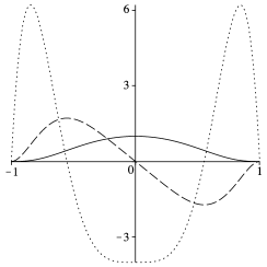
Figure 5: The window function (46) (black line) and its first (dashed line) and second (dotted line) derivatives. Each of these three functions sample the interval $[-1,1]$ visibly uniformly enough (not particularly favouring some parts of the interval over other parts).

The integral of any data series was calculated numerically, but here we also wanted to improve the performance. The reason for this is that, in many cases in practice, one has only a few dozens of data points at hand. We need to consider at least five different intervals for determining the five unknown constants, or, if we also want some error bars for the determined constants then at least seven intervals are preferable. Then the numerical integrals need to be fairly reliable since their values will not differ too much, with the danger of numerical unreliability.

To this end, we have modified the classic trapezoidal rule for numerical integration. Namely, the trapezoidal rule approximates the integrand by a linear function (piecewise). However, in our case, a product is to be integrated, and the second derivative of our window function changes unavoidably rapidly. This itself invalidates the (piecewise) linear approximation considerably. The idea then is to approximate only the data itself by linear pieces, and to treat the window function (or its appropriate derivative) in an exact manner. For example,

$$\int_{t_{a}}^{t_{b}}\sigma^{\rule{0.20999pt}{2.71246pt}\kern 0.41998pt\rule{0.20999pt}{2.71246pt}}(t)w(t)\mathrm{d}t$$ (47)

$$\approx\int_{ta1}^{t_{b}}\left[\sigma^{\rule{0.20999pt}{2.71246pt}\kern 0.41998pt\rule{0.20999pt}{2.71246pt}}(t_{a})+\frac{\sigma^{\rule{0.20999pt}{2.71246pt}\kern 0.41998pt\rule{0.20999pt}{2.71246pt}}(t_{b})-\sigma^{\rule{0.20999pt}{2.71246pt}\kern 0.41998pt\rule{0.20999pt}{2.71246pt}}(t_{a})}{t_{b}-t_{a}}\left(t-t_{a}\right)\right]w(t)\mathrm{d}t,$$

the calculation of which going back to the integral of $w(t)$ and of $tw(t)$, which both we can determine exactly.

After these preparations, data behaving like those in Fig. 4a proved to be treatable. For rheological constants, such parts of a time series are informative where the data changes well enough so that its second derivative also changes well enough. For demonstration, we show here the fitting for just a small part of the first loading-unloading cycle on Fig. 4a: the ending part of the loading and the beginning part of the unloading. The abrupt change from loading to unloading may seem dangerous to use but is actually most informative for rheological parameters, which manifest themselves the best during heavy changes.

The least-squares fitting provides us error bars and an $R^{2}$ value can also be calculated to quantify the goodness of the fit, still, the best is when one can also visualize the quality of the fit. To this end, solving the simple numerical scheme

$$\sigma^{\text{sph}}_{n} +\tau^{\text{sph}}\frac{\sigma^{\text{sph}}_{n\vphantom{1}}-\sigma^{\text{sph}}_{n-1}}{\Delta t}$$

$$=\delta^{\text{sph}}+E_{0}^{\text{sph}}\varepsilon^{\text{sph}}_{n}+E_{1}^{\text{sph}}\frac{\varepsilon^{\text{sph}}_{n\vphantom{1}}-\varepsilon^{\text{sph}}_{n-1}}{\Delta t}$$

$$+E_{2}^{\text{sph}}\frac{\varepsilon^{\text{sph}}_{n+1}-2\varepsilon^{\text{sph}}_{n\vphantom{1}}+\varepsilon^{\text{sph}}_{n-1}}{\Delta t^{2}}$$ (48)

for $\sigma^{\text{sph}}_{n}$, we predicted $\sigma^{\text{sph}}$ values from experimental $\varepsilon^{\text{sph}}$ values and an initial $\sigma^{\text{sph}}$ value (and treated the deviatoric counterpart analogously). An advantage of this scheme is that it is reliably applicable even if some of the fitted coefficients are small, or are known to be zero a priori.

As mentioned, we present here the result for just a small part of the process, in order to exhibit the quality of the established numerical approach. Thirty data points are used, and integration is done on seven intervals. This way, each interval consists of only six points. (Neighbouring intervals have an overlap of two points.) Apparently, six points means a rude discretization for an integral on an interval so such a situation is a good test of the numerical method. The obtained fitted coefficients and the predictions based on them can be seen in Table 1 and Fig. 6.

material	fitted	standard
parameter	value	error
$\tau^{\text{dev}}[\text{s}]$	0.3600	$\pm 0.0659$ $|^{|}_{+}$
$E_{0}^{\text{dev}}[\text{GPa}]$	0.8612	$\pm 0.0556$ $|^{|}_{+}$
$E_{1}^{\text{dev}}[\text{GPa}\cdot\text{s}]$	0.4724	$\pm 0.0686$ $|^{|}_{+}$
$E_{2}^{\text{dev}}[\text{GPa}\cdot\text{s}^{2}]$	0.0029	$\pm 0.0010$ $|^{|}_{+}$
$\tau^{\text{sph}}[\text{s}]$	0.2329	$\pm 0.0904$ $|^{|}_{+}$
$E_{0}^{\text{sph}}[\text{GPa}]$	4.5708	$\pm 1.0392$ $|^{|}_{+}$
$E_{1}^{\text{sph}}[\text{GPa}\cdot\text{s}]$	1.8566	$\pm 0.4401$ $|^{|}_{+}$
$E_{2}^{\text{sph}}[\text{GPa}\cdot\text{s}^{2}]$	0.0013	$\pm 0.0220$ $|^{|}_{+}$

Table 1: Table of fitted rheological coefficients for the deviatoric and spherical parts

(a)  (b)

Figure 6: Comparison of the theoretical prediction based on the values of Table 1 (solid line) to the experimental stress data (points). For information, the measured strain values (circles) are also displayed (rescaled appropriately). Horizontal axes: time in s, vertical axes: stress in MPa. (a) Deviatoric case. (b) Spherical case.

Various further checks can be made for the determined rheological coefficients. First, it is reassuring to find that the thermodynamical constraints (39)–(42) are fulfilled. Second, the elastic constants $E_{0}^{\text{dev}}$, $E_{0}^{\text{sph}}$ enable to calculate Poisson’s ratio and Young’s modulus (see Appendix A of [12]). The resulting former value (0.37) coincides nicely with the literature data (0.38). Young’s modulus (1.2 GPa) comes out somewhat below the typical literature range (1.9 GPa $\sim$ 3.3 GPa) which, however, depends heavily on humidity (that’s why the literature range is so wide). In parallel, one must bear in mind that customary measurements of Young’s modulus are performed at finite loading speeds where the steepness of the longitudinal stress–strain curve is seriously influenced by rheology. For example, even for the simplest rheological situation, a Kelvin–Voigt model in the deviatoric part and a Hooke model in the spherical part, the uniaxial equation contains not only $\sigma^{\rule{0.20999pt}{2.71246pt}\kern 0.41998pt\rule{0.20999pt}{2.71246pt}}$ and $\varepsilon^{\rule{0.20999pt}{2.71246pt}\kern 0.41998pt\rule{0.20999pt}{2.71246pt}}$ but also their first time derivative, too ([12], Appendix A). The ratio of these derivatives, $\dot{\sigma}^{\rule{0.20999pt}{2.71246pt}\kern 0.41998pt\rule{0.20999pt}{2.71246pt}}/\dot{\varepsilon}^{\rule{0.20999pt}{2.71246pt}\kern 0.41998pt\rule{0.20999pt}{2.71246pt}}$, dominates the slope of the longitudinal stress–strain curve at the beginning of the loading and, for not too slow loading, the later part as well. In other words, the ratio of the coefficients of these first derivatives (in systematic notation, ${E_{1}}^{\rule{0.20999pt}{2.71246pt}\kern 0.41998pt\rule{0.20999pt}{2.71246pt}}/{\tau_{1}}^{\rule{0.20999pt}{2.71246pt}\kern 0.41998pt\rule{0.20999pt}{2.71246pt}}$) plays the role of a dynamical Young’s modulus. Now, for the rheological coefficients found by the above fit, this dynamical Young’s modulus turns out to be 1.47 GPa, 24% higher than the static one. We remark that, as a consequence of the thermodynamical inequalities (39)–(42), the dynamical Young’s modulus is always larger than the static one [12]. For more complicated rheologies – like the one we have here – even higher order dynamical Young’s moduli are present (ratios of coefficients of higher derivatives). The second order dynamical Young’s modulus, for example, is already 1.84 GPa.

It is a generally valid warning from the rheology of solids that customary ways of extracting Young’s modulus from longitudinal stress–strain curves may result in erroneously high values whenever rheology is neglected. Notably, it is not only plastics [22] and similar materials where one may encounter rheology in solids: as an important application, the mechanical description of rocks also requires the full rheological model, as exploited in the ASR (Anelastic Strain Recovery) method for determining 3D in situ stress (see [23, 24, 25]).

8 Discussion

The presented theory is rich in the sense that it grasps the elastic, thermal expansion, thermal conduction, rheological and plastic aspects of solids. On the other side, for each of these aspects, the simplest available kinematic and constitutive choices have been made here, in order to make the comparison with experimental data easy. These specific choices have been found to be in conform with the experiments that we have performed for illustration. The framework is nevertheless general enough to describe much more general processes and material behaviours as well, such as large deformation processes, material anisotropy, nonlinear elasticity, elaborated plastic effects, and all with nonconstant elasticity, thermal expansion, rheological and other coefficients.

As for feasible future generalizations of the theory, first, one can mention allowing the Onsagerian coupling between the plastic and the rheological side as well. Second, non-Fourier heat conduction can also be incorporated, unifying the internal variable approach [11] for rigid heat conductors with the thermomechanical side described here. Damage and failure [26, 27] are more distant but also reasonable candidates to include via the same thermodynamical methodology, along the lines of the works [9, 10]. Temperature dependent complicated rheological/viscoelastic situations in the finite deformation regime [28] mean further challenges.

On the experimental side, our intention here was to present examples for the involved various aspects. These aspects, such as the Joule-Thomson effect and the Kluitenberg–Verhás rheology, have been found to be in good quantitative agreement with the theory. In the future, with higher precision and higher reliability measurements of the kind performed here, a full quantitative agreement can be achieved. For example, already the present data allows us to approximately identify the plastic yield stress value to be around 100 MPa (the stress level where the transient takes place in Fig. 4a and temperature starts showing plastic dissipation), and the ratio of the steepnesses before and after the plastic yield leads to an approximate prediction of the plastic rate coefficient [$\gamma\approx 0.17$ in (22)] but a more elaborate approach is desirable. If the experimental setup is able to provide fast enough loading and unloading –needed for studying rheology precisely – while all strain, force and temperature values are measured with high precision and reliability then, after fitting all the material constants involved, the numerical scheme explained in Sect. 5 (and extended to also include thermal expansion and plasticity) should be able to reproduce the whole time series precisely.

In addition to discussing the numerical scheme for predicting the time dependence of quantities, we have presented a method for fitting the rheological coefficients, which succeeded in this task satisfactorily. We have emphasized the importance of having transversal strain to be also measured, since this reduces the labour of fitting significantly, enabling to divide the problem into two separate, easily treatable, halves (deviatoric and spherical), while the composite uniaxial eight-parameter situation may be found practically intractable.

Besides monitoring the mechanical quantities, measuring temperature provides valuable additional information about the process of solid samples. The elastic, rheological and plastic aspects make a clear footprint on the temperature time series as well. Actually, because of the inherent intertwining of thermal and mechanical aspects, the set of equations is closed only when the temperature variable is a full member of the set of variables. The thermodynamics-based approach enlights the importance of temperature for processes that are traditionally treated as mechanical-only.

The analysis of the experimental data has clearly shown the relevance of rheology for plastics, and the situation is known to be the same for seemingly more ”solid” solids like rocks [23, 24, 25], which is the base of the above-mentioned ASR method for determining 3D in situ stress. What seems nonlinear elasticity in the stress–strain plane may well be rheology. However, another important remark to be made is that delays in an experimental equipment (implementation of loading, controlling, measuring devices etc.) should not confused with rheological delays acting within the sample. Much experimental care is needed, in parallel to the proper theoretical interpretation, to identify the presence of true rheology in solids. The applicational consequences of reliable rheological information are far-reaching (the long-time behaviour of underground tunnels, safety aspects of structural materials etc.). The interplay between thermal, elastic and rheological effects is also remarkably important. The thermodynamics-based description of solids provides a reliable theoretical framework for all these phenomena.

Appendix A Technical details of the measurement

The measurements have been carried out with an Instron 5581 universal material tester device, at the Hungarian Institute of Agricultural Engineering. The arrangement can be seen in Fig. 7.

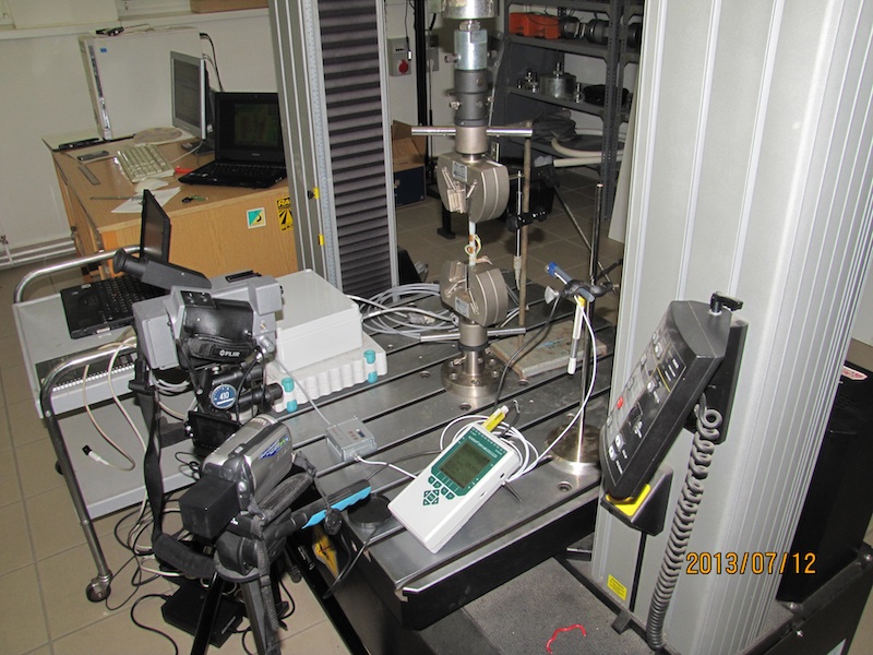
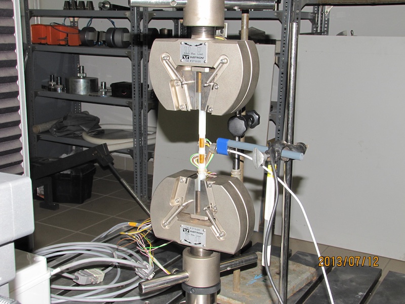
Figure 7: The measuring arrangement

To track the longitudinal and lateral size changes of the tested sample, a tensiometric measuring device was used. HBM 3/350 XY11 type strain gauge was mounted onto the specimen (Fig. 8). The resistance of the gauge is $R=350\Omega$, and the gauge factor is $k=1.98$ (1%, according to the technical parameters provided by the supplier.)

Figure 8: Strain gauge used for the measurement

Half bridge was used to test the specimen. The active gauge was the one mounted on the specimen, while the other gauge of the bridge was mounted on an unloaded metal plate. During the measurements, the half bridge was connected to an SR-55 radio frequency module of a Spider-8 amplifier.

A ThermaCAM PM695 type real-time thermal camera was used for temperature measurement and imaging. It monitored the area of the specimen indicated by dashed lines in Fig. 2. Besides the average temperature of the area and the maximal temperature value within the area, the temperature value at two fixed spots were also registered. In parallel, temperature at some additional spots was monitored via infrared temperature sensor (supplier: Optrics GmbH, type: OPTCTLT10FCB3).

Standard specimens were used. After manufacturing, the specimens were relieved from load, and were calibrated after the gauges were mounted. The geometric dimensions of the specimen are displayed in Fig. 2.

References

- [1] T. Fülöp and P. Ván. Kinematic quantities of finite elastic and plastic deformation. Math. Meth. Appl. Sci., 35:1825–1841, 2012.
- [2] T. Fülöp. Thermal expansion, elastic stress and finite deformation kinematics. In 10th International Conference on Heat Engines and Environmental Protection, 23–25 May 2011, Balatonfüred, Hungary, pages 227–232, Budapest, 2011. Budapest University of Technology and Economics, Department of Energy Engineering.
- [3] T. Fülöp, P. Ván, and A. Csatár. Elasticity, plasticity, rheology and thermal stress – an irreversible thermodynamical theory. In M. Pilotelli and G. P. Beretta, editors, 12th Joint European Thermodynamics Conference, JETC 2013, Brescia, Italy, July 1–5, 2013, pages 525–530, Brescia, 2013. Snoopy.
- [4] T. Fülöp, P. Ván, and A. Csatár. Thermodynamical description of plastic processes. In Gy. Gróf, editor, 11th International Conference on Heat Engines and Environmental Protection, June 3–5, 2013, Balatonfüred, Hungary, pages 147–152, Budapest, 2013. University of Technology and Economics, Department of Energy Engineering.
- [5] T. Matolcsi. A Concept of Mathematical Physics: Models for Spacetime. Akadémiai Kiadó, Budapest, 1984.
- [6] T. Matolcsi. Spacetime Without Reference Frames. Akadémiai Kiadó, Budapest, 1993.
- [7] T. Matolcsi. On material frame-indifference. Arch. Rational Mech. Anal., 91:99–118, 1986.
- [8] T. Matolcsi and T. Gruber. Spacetime without reference frames: An application to the kinetic theory. International Journal of Theoretical Physics, 35:1523–1539, 1996.
- [9] P. Ván. Internal thermodynamic variables and the failure of microcracked materials. Journal of Non-Equilibrium Thermodynamics, 26:167–189, 1996.
- [10] P. Ván and B. Vásárhelyi. Second Law of thermodynamics and the failure of rock materials. In D. Elsworth, J. P. Tinucci, and K. A. Heasley, editors, Rock Mechanics in the National Interest: Proceedings of the 9th North American Rock Mechanics Symposium, Washington, USA, 2001, pages 767–773, Lisse, Abingdon, Exton (PA), Tokyo, 2001. Balkema Publishers.
- [11] P. Ván and T. Fülöp. Universality in heat conduction theory: Weakly nonlocal thermodynamics. Annalen der Physik, 524:470–478, 2012.
- [12] Cs. Asszonyi, T. Fülöp, and P. Ván. Distinguished rheological models in the framework of a thermodynamical internal variable theory. Continuum Mechanics and Thermodynamics, 2014. First online: 20 November 2014.
- [13] P. Neff, B. Eidel, F. Osterbrink, and R. Martin. A Riemannian approach to strain measures in nonlinear elasticity. Comptes Rendus de l’Académie des Sciences, 342:254–257, 2014.
- [14] P. Neff, I. D. Ghiba, and J. Lankeit. The exponentiated Hencky-logarithmic strain energy. Part I: Constitutive issues and rank-one convexity. Journal of Elasticity, 2015. First online: 27 March 2015.
- [15] M. F. Beatty and D. O. Stalnaker. The Poisson function of finite elasticity. Journal of Applied Mechanics, 108:807–813, 1986.
- [16] C. O. Horgan and J. G. Murphy. A generalization of Hencky’s strain-energy density to model the large deformations of slightly compressible solid rubber. Mechanics of Materials, 79:943–950, 2009.
- [17] J. Plešek and A. Kruisová. Formulation, validation and numerical procedures for Hencky’s elasticity model. Computers and Structures, 84:1141–1150, 2006.
- [18] O. T. Bruhns, H. Xiao, and A. Mayers. Constitutive inequalities for an isotropic elastic strain energy function based on Hencky’s logarithmic strain tensor. Proceedings of the Royal Society of London A, 457:2207–2226, 2001.
- [19] A. Rusinko and K. Rusinko. Plasticity and Creep of Metals. Springer-Verlag, Berlin Heidelberg, 2011.
- [20] V. A. Lubarda. On thermodynamic potentials in linear thermoelasticity. International Journal of Solids and Structures, 41:7377–7398, 2004.
- [21] J. Verhás. Thermodynamics and Rheology. Akadémiai Kiadó and Kluwer Academic Publisher, Budapest, 1997.
- [22] D. Kocsis and R. Horváth. Experience acquired in tensile tests of plastics. Scientific Bulletin Series C: Fascile Mechanics, Tribology, Machine Manufacturing Technology, 27, 2013.
- [23] K. Matsuki and K. Takeuchi. Three-dimensional in situ stress determination by anelastic strain recovery of a rock core. International Journal of Rock Mechanics and Mining Sciences & Geomechanics Abstracts, 30:1019–1022, 1993.
- [24] K. Matsuki. Anelastic strain recovery compliance of rocks and its application to in situ stress measurement. International Journal of Rock Mechanics and Mining Sciences, 45:952–965, 2008.
- [25] W. Lin, Y. Kuwahara, T. Satoh, N. Shigematsu, Y. Kitagawa, T. Kiguchi, and N. Koizumi. A case study of 3D stress orientation determination in Shikoku Island and Kii Peninsula, Japan. In I. Vrkljan, editor, Rock Engineering in Difficult Ground Conditions (Soft Rock and Karst), Proceedings of Eurock’09 Cavtat, Croatia, October 28–29, 2009, pages 277–282. Balkema, 2010.
- [26] P. Ván and B. Vásárhelyi. Sensitivity analysis of GSI based mechanical parameters of the rock mass. Periodica Polytechnica–Civil Engineering, 58:379–386, 2014.
- [27] F. Deák, P. Ván, and B. Vásárhelyi. Hundred years after the first triaxial test. Periodica Polytechnica–Civil Engineering, 56:115–122, 2012.
- [28] L. Pálfi and K. Váradi. Characterization and implementation of the viscoelastic properties of an EPDM rubber into FEA for energy loss prediction. Period. Polytech. Mech. Eng., 54:35–40, 2010.