Analyticity of the Dirichlet-to-Neumann map for the time-harmonic Maxwell’s equations

Abstract

In this chapter we derive the analyticity properties of the electromagnetic Dirichlet-to-Neumann map for the time-harmonic Maxwell’s equations for passive linear multicomponent media. Moreover, we discuss the connection of this map to Herglotz functions for isotropic and anisotropic multicomponent composites.

Key words: multicomponent media, electromagnetic Dirichlet-to-Neumann map, analytic properties, Herglotz functions

1 Introduction

In this chapter, we study the analytic properties of the electromagnetic “Dirichlet-to-Neumann” (DtN) map for a composite material. Using passive linear multicomponent media, we will prove that this DtN map is an analytic function of the dielectric permittivities and magnetic permeabilities (multiplied by the frequency $\omega$) which characterize each phase. More specifically, it belongs to a special class of functions known as Herglotz functions. In that sense, this chapter is highly connected to the previous one by Graeme Milton since both are proving analyticity properties on the DtN map, but with different methods. In [Milton 2016, Chapter 3], these analyticity properties are derived by using the theory of composite materials, whereas in this chapter they are proved via spectral theory in the usual functional framework associated with the time-harmonic Maxwell’s equations. Maxwell’s equations at fixed frequency $\omega$ involve the electric permittivity $\varepsilon({\bf x},\omega)$ (also called the dielectric constant if measured relative to the permittivity of the vacuum) and the magnetic permeability $\mu({\bf x},\omega)$. The approach taken in the current chapter has the important advantage of being applicable to bodies where the moduli $\omega\varepsilon({\bf x},\omega)$ and $\omega\mu({\bf x},\omega)$ are not piecewise constant but instead vary smoothly (or not) with position. In this case we establish (in Subsection 3.4) the Herglotz properties of the Dirichlet-to-Neumann map, as a function of frequency, assuming the material is passive at each point ${\bf x}$, i.e., that $\omega\varepsilon({\bf x},\omega)$ and $\omega\mu({\bf x},\omega)$ are Herglotz functions of the frequency $\omega$.

The use of theory of Herglotz functions in electromagnetism and in the theory of composites has many important impacts and consequences (Bergman ?, ?, ?; Milton ?, ?, ?, ?; [Golden and Papanicolaou 1983]; [Dell’Antonio, Figari, and Orlandi 1986]; [Bruno 1991]; Lipton ?, ?; [Gustafsson and Sjöberg 2010]; [Bernland, Luger, and Gustafsson 2011]; [Liu, Guenneau, and Gralak 2013]; [Welters, Avniel, and Johnson 2014]) especially in developing bounds on certain physical quantities. Based on this and the work of ?), ?), Milton (?, ?) and ?) on developing bounds on effective tensors of composites containing more than two phases using analyticity of the effective tensors as a multivariable function of the moduli of the phases, we also establish that the DtN map is an analytic function of the permittivity and permeability tensors of each phase. Another potential application of these analytic properties is to derive information about the DtN map for real frequencies by using the theory of boundary-values of Herglotz functions (for instance, see [Gesztesy and Tsekanovskii 2000] and [Naboko 1996]). Moreover, as the DtN map is usually used as data in electromagnetic inverse problems (see, for instance, [Albanese and Monk 2006]; [Uhlmann and Zhou 2014], [Ola, P iv rinta, and Somersalo 2012]), we believe these analyticity properties and the connection to the theory of Herglotz functions will have important applications in this area of research (see [Milton 2016, Chapter 5]). The Herglotz properties might also be important to characterize the complete set of all possible Dirichlet-to-Neumann maps (either at fixed frequency or as a function of frequency) associated with multiphase bodies with frequency independent permittivity and permeability. Indeed such analyticity properties were a key ingredient to characterize the possible dynamic response functions of multiterminal mass-spring networks ([Guevara Vasquez, Milton, and Onofrei 2011]). These response functions are the discrete analogs of the Dirichlet-to-Neumann map in that problem. Additionally, analytic properties were a key ingredient in the theory of exact relations ([Grabovsky 1998]; [Grabovsky and Sage 1998]; [Grabovsky, Milton, and Sage 2000]: see also Chapter 17 in [Milton 2002] and [Grabovsky 2004]) satisfied by the effective tensors of composites, and for establishing links between effective tensors. These are generally nonlinear relations that are microstructure independent and thus, besides their intrinsic interest, are useful as benchmarks for numerical methods and approximations. They become linear ([Grabovsky 1998]) after a suitable fractional linear matrix transformation is made (which is nonunique and involves an arbitrary unit vector ${\bf n}$). After any such transformation is made and once certain algebraic relations are satisfied (for all unit vectors ${\bf n}$) it can be proved that all terms in the series expansion satisfy the exact relation, and then analyticity is needed to prove the relation holds (in the domain of analyticity) even if the series expansion does not converge ([Grabovsky, Milton, and Sage 2000]).

We split this chapter in three sections. In the first one, we consider the electromagnetic DtN map for a layered media. In this setting, the DtN map can be expressed explicitly in terms of the transfer matrix associated with the medium. This gives a good example in which one can see these analytic properties in the context of matrix perturbation theory ([Baumgärtel 1985]; [Kato 1995]; [Welters 2011a]). In the second section, we restrict ourselves to bounded media but with a large class of different geometries, more precisely, Lipschitz domains. In this case, using a variational reformulation of the time-harmonic Maxwell’s equations ([Cessenat 1996]; [Kirsch and Hettlich 2015]; [Monk 2003]; [Nedelec 2001]), we prove both the well-posedness and the analyticity of the DtN map. Also we consider bodies where the moduli $\omega\varepsilon({\bf x},\omega)$ and $\omega\mu({\bf x},\omega)$ are not piecewise constant but instead vary with position, and at each point ${\bf x}$ are Herglotz functions of the frequency $\omega$. In this case we establish the Herglotz properties of the Dirichlet-to-Neumann map, as a function of frequency. In both sections, the key step to prove the multivariable analyticity is Hartogs’ Theorem from complex analysis which essentially says that analyticity in each variable separately implies joint analyticity (see Theorem 4 below). Concerning the connection to Herglotz functions, an energy balance equation is derived (which is essentially Poynting’s Theorem for complex frequencies) that allows us to prove that the imaginary part of the DtN map is positive definite, as a consequence of the positivity of the imaginary part of the material tensors. Nevertheless, in the case of anisotropic media, the connection to Herglotz functions has to be made more precise. Indeed, we leave here the usual framework of Herglotz functions of scalar variables since we are concerned with dielectric permittivity and magnetic permeability tensors as input variables. Thus, the purpose of the last section is to provide a rigorous definition of Herglotz functions in this general framework, that provides an alternative to the one developed in Section 18.8 of ?), by connecting this notion to the theory of holomorphic functions on tubular domains with nonnegative imaginary part as described in [Vladimirov 2002] (see Sections $17$–$19$). This new link is especially significant since this class of functions (like the Herglotz functions introduced in Section 18.8 of ?)) admits integral representations analogous to Herglotz functions of one complex variable (the representation in the one variable case as described in Theorem 3 below) and are deeply connected to the theory of multivariate passive linear systems (see Section $20$ in [Vladimirov 2002]) with the notions of convolutions, passivity, causality, Laplace/Fourier transforms, and analyticity properties.

This chapter is essentially self-contained, and written in a rigorous mathematical style. Care has been taken to explain most technical definitions so that it should be accessible to non-mathematicians.

Before we proceed, let us introduce some notation, definitions and theorems used in this chapter. We denote:

• the complex upper-half plane by ${\mathbb{C}}^{+}=\left\{z\in{\mathbb{C}}\mid\operatorname{Im}z>0\right\}$,

• the Banach space of all $m\times n$ matrices with complex entries by $M_{m,n}({\mathbb{C}})$ equipped with any norm, with the square matrices $M_{n,n}({\mathbb{C}})$ denoted by $M_{n}({\mathbb{C}})$, and we treat ${\mathbb{C}}^{n}$ as $M_{n,1}({\mathbb{C}})$ (recall that a Banach space is a complete normed vector space: unlike a Hilbert space, it does not necessarily have an inner product defined on the space, just a norm.)

• by $\cdot$ the operation defined for all vectors ${\bf u},{\bf v}\in{\mathbb{C}}^{n}$ via ${\bf u}\cdot\,{\bf v}={\bf u}^{T}{\bf v}=u_{i}v_{i}$, where $T$ denotes the transpose. Note that there is no complex conjugation in this definition, so ${\bf u}\cdot{\bf u}$ is not generally real.

• the open, connected, and convex subset of $M_{n}({\mathbb{C}})$ of matrices with positive definite imaginary part by

  $$M_{n}^{+}({\mathbb{C}})=\left\{{\bf M}\in M_{n}({\mathbb{C}})\mid\operatorname{Im}{\bf M}>0\right\},$$

  where $\operatorname{Im}{\bf M}=({\bf M}-{\bf M}^{*})/(2i)$ with ${\bf M}^{*}=\overline{{\bf M}}^{T}$ the adjoint of ${\bf M}$, and the inequality ${\bf M}>0$ holds in the sense of quadratic forms. We remark that this set is invariant by the operation: ${\bf M}\to-{\bf M}^{-1}$ since if ${\bf M}\in M_{n}^{+}({\mathbb{C}})$ then ${\bf M}$ is invertible and

  $$-\operatorname{Im}({\bf M}^{-1})=({\bf M}^{-1})^{*}\,\operatorname{Im}({\bf M})\,{\bf M}^{-1}>0$$

• by $L(E,F)$ the Banach space of all continuous linear operators from a Banach space $E$ to a Banach space $F$ equipped with the operator norm.

Definition 1.

(Analyticity) Let $E$ and $F$ be two complex Banach spaces and $U$ be an open set of $E$. A function $f:U\to F$ is said to be a analytic if it is differentiable on ${\cal U}$.

Definition 2.

(Herglotz functions) Let $m,n,N\in\mathbb{N}$, where $\mathbb{N}$ is the set of natural numbers (positive integers), and $\mathcal{T}=({\mathbb{C}}^{+})^{n}$ or $(M_{N}^{+}({\mathbb{C}}))^{n}$. An analytic function $h:\mathcal{T}\to{\mathbb{C}}$ or $h:\mathcal{T}\to M_{m}({\mathbb{C}})$ is called a Herglotz function (also called Pick or Nevanlinna function) if

$$\operatorname{Im}(h({\bf z}))\geq 0,\ \forall{\bf z}\in\mathcal{T}.$$

We note here that Definition 2 is the standard definition of a Herglotz function when $\mathcal{T}={\mathbb{C}}^{+}$ (see [Gesztesy and Tsekanovskii 2000], [Berg 2008]) and $\mathcal{T}=({\mathbb{C}}^{+})^{n}$ (in [Agler, McCarthy, and Young 2012] it is called a Pick function), but not when $\mathcal{T}=(M_{N}^{+}({\mathbb{C}}))^{n}$. Its justification in this last case is given in Section 4.

A particular and useful property of Herglotz functions defined on a scalar variable, which has been a key-tool to use analytic methods to derive bounds, is the following representation theorem.

Theorem 3.

A necessary and sufficient condition for a function $h:{\mathbb{C}}^{+}\to{\mathbb{C}}$ to be a Herglotz function is that there exist $\alpha,\beta\in{\mathbb{R}}$ with $\alpha\geq 0$ and a positive regular Borel measure $\mu$ for which $\int_{{\mathbb{R}}}\ {\rm d}\mu(\lambda)/(1+\lambda^{2})$ is finite such that

$$h(z)=\alpha\,z+\beta+\displaystyle\int_{{\mathbb{R}}}\left(\frac{1}{\lambda-z}-\frac{\lambda}{1+\lambda^{2}}\right){\rm d}\mu(\lambda),\ \mbox{ for }z\in{\mathbb{C}}^{+}.$$ (1.1)

For an extension of this representation theorem, for instance, in the case of matrix-valued Herglotz functions $h:{\mathbb{C}}^{+}\to M_{m}({\mathbb{C}})$, we refer to ?).

Theorem 4.

(Hartogs’ Theorem) If $h:U\to E$ is a function with $U$ an open subset of ${\mathbb{C}}^{n}$ and $E$ is a Banach space then $h$ is a multivariate analytic function (i.e., jointly analytic) if and only if it is an analytic function of each variable separately.

A proof of Hartogs’ Theorem when $E={\mathbb{C}}$ can be found in ?) (see Section  2.2, p. 28, Theorem 2.2.8). For the general case, we refer the reader to ?) (see Section 36, p. 265, Theorem 36.1).

Theorem 5.

Let $E$ and $F$ denote two Banach spaces and $U$ an open subset of ${\mathbb{C}}^{n}$. If $h:U\to L(E,F)$ is an analytic function and for each ${\bf z}\in U$ the value $h({\bf z})$ is an isomorphism, then the function ${\bf z}\to h({\bf z})^{-1}$ is analytic from $U$ into $L(F,E)$.

For a proof of Theorem 5 when $n=1$, we refer the reader to ?) (see Chapter 7, Section 1, pp. 365–366). The proof for an integer $n>1$ is then obtained by using Hartogs’ Theorem.

The next theorem, which is a rewriting of Theorem 3.12 of ?) shows that the notion of weak analyticity of a family of operators in $L(E,F)$ implies the analyticity of this family for the operator norm of $L(E,F)$. More precisely, we have the following result:

Theorem 6.

Let $E$ and $F$ be two Banach spaces, $U$ an open subset of ${\mathbb{C}}$ and $h:U\to L(E,F)$. We denote by $\left\langle\cdot,\cdot\right\rangle$ the duality product of $F$ and its dual $F^{*}$. If the function

$$h_{\phi,\psi}(z)=\left\langle h(z)\phi,\psi\right\rangle,\,\forall z\in U,$$

is analytic on $U$ for all $\phi$ in a dense subset of $E$ and for all $\psi$ in a dense subset of $F^{*}$, then $h$ is analytic in $U$ for the operator norm of $L(E,F)$.

The following is a theorem for taking the derivative under the integral of a function which depends analytically on a complex parameter (see [Mattner 2001]). It introduces the notion of a measure space that we briefly recall here. A measure space $(\Omega,\mathcal{F},\mu)$ is roughly speaking a triple composed of a set $\Omega$, a collection $\mathcal{F}$ of subsets of $\Omega$ that one wants to measure ($\mathcal{F}$ is called a $\sigma-$algebra) and a measure $\mu$ defined on $\mathcal{F}$.

Theorem 7.

Let $(\Omega,\mathcal{F},\mu)$ be a measure space, let $U$ be an open set of ${\mathbb{C}}$ and $f:\Omega\times U\to{\mathbb{C}}$ be a function subject to the following assumptions:

• $f(\cdot,z)$ is $\mathcal{F}$ measurable for all $z\in U$ and $f({\bf x},\cdot)$ is analytic for almost every ${\bf x}$ in $\Omega$,

• $\int_{\Omega}|f({\bf x},\cdot)|\,\mathrm{d}\mu({\bf x})$ is locally bounded, that is, for every $z_{0}\in U$ there exists a $\delta>0$ such that

  $$\sup_{z\in U\mid|z-z_{0}|\leq\delta}\int_{\Omega}|f({\bf x},z)|\,\mathrm{d}\mu({\bf x})<\infty,$$

then the function $F:U\to{\mathbb{C}}$ defined by

$$F(z)=\int_{\Omega}f({\bf x},z)\,\mathrm{d}\mu({\bf x}),$$

is analytic in $U$ and one can take derivatives under the integral sign:

$$F^{(k)}(z)=\int_{\Omega}\frac{\partial^{k}f({\bf x},z)}{\partial z^{k}}\,\mathrm{d}\mu({\bf x}),\ \forall k\in\mathbb{N}.$$

2 Analyticity of the DtN map for layered media

2.1 Formulation of the problem

We consider passive linear two-component layered media (material 1 with moduli $\mbox{\boldmath${\varepsilon}$}_{1},\mbox{\boldmath${\mu}$}_{1}$; material 2 with moduli $\mbox{\boldmath${\varepsilon}$}_{2},\mbox{\boldmath${\mu}$}_{2}$) with layers normal to the $z$-axis. The geometry of this problem, as illustrated in 1, is as follows: First, a layered medium in the region $\Omega=\Omega_{1}\cup\Omega_{2}=[-d,d]$ consisting of a two-phase material lies between $z=-d$ and $z=d$. A homogeneous passive linear material lies between $-d_{2}\leq z\leq d_{2}$ (denote this “inner” region by $\Omega_{2}=[-d_{2},d_{2}]$) with permittivity and permeability $\mbox{\boldmath${\varepsilon}$}_{2},\mbox{\boldmath${\mu}$}_{2}$. Another homogeneous passive linear material lies between $-d\leq z<-d_{2}$, i.e., the region $\Omega_{1,-}=[-d,-d_{2})$, and $d_{2}<z\leq d$, i.e., the region $\Omega_{1,+}=(d_{2},d]$ (denote “outer” region by $\Omega_{1}=\Omega_{1,-}\cup\Omega_{1,+}$) with permittivity and permeability $\mbox{\boldmath${\varepsilon}$}_{1},\mbox{\boldmath${\mu}$}_{1}$. The unit outward pointing normal vectors to the boundary surfaces of these regions are $\textbf{n}\in\{\textbf{e}_{3},-\textbf{e}_{3}\}$, where $\textbf{e}_{3}=\begin{bmatrix}0&0&1\end{bmatrix}^{T}$.

The dielectric permittivity ${\varepsilon}$ and magnetic permeability ${\mu}$ are $3\times 3$ matrices that depend on the frequency $\omega$ and the spatial variable $z$ only (i.e., spatially homogeneous in each layer) which are defined by

$$\mbox{\boldmath${\varepsilon}$}=\mbox{\boldmath${\varepsilon}$}(\omega,z)=\chi_{\Omega_{1}}(z)\mbox{\boldmath${\varepsilon}$}_{1}(\omega)+\chi_{\Omega_{2}}(z)\mbox{\boldmath${\varepsilon}$}_{2}(\omega),\;\;z\in[-d,d],\;\omega\in{\mathbb{C}}^{+},$$ (2.1)

$$\mbox{\boldmath${\mu}$}=\mbox{\boldmath${\mu}$}(\omega,z)=\chi_{\Omega_{1}}(z)\mbox{\boldmath${\mu}$}_{1}(\omega)+\chi_{\Omega_{2}}(z)\mbox{\boldmath${\mu}$}_{2}(\omega),\;\;z\in[-d,d],\;\omega\in{\mathbb{C}}^{+}.$$ (2.2)

Here $\chi_{\Omega_{j}}$ denotes the indicator function of the region $\Omega_{j}$, for $j=1,2$. Moreover, they have the passivity properties [see, for example, [Milton 2016, Section 1.6]]

$$\operatorname{Im}(\omega\mbox{\boldmath${\varepsilon}$}(\omega,z))>0,\;\;\operatorname{Im}(\omega\mbox{\boldmath${\mu}$}(\omega,z))>0,\;\textnormal{for }\operatorname{Im}\omega>0,$$ (2.3)

and $\mbox{\boldmath${\varepsilon}$},\mbox{\boldmath${\mu}$}$ are analytic functions of $\omega$ in the complex upper-half plane for each fixed $z$, i.e.,

$$\omega\mbox{\boldmath${\varepsilon}$}_{j}(\omega),\omega\mbox{\boldmath${\mu}$}_{j}(\omega):{\mathbb{C}}^{+}\rightarrow M_{3}^{+}({\mathbb{C}})\textnormal{ are Herglotz functions, for }j=1,2.$$ (2.4)

The time-harmonic Maxwell’s equations in Gaussian units without sources are

$$\mathrm{curl\,}\textbf{E}=\frac{i\omega}{c}\textbf{B},\;\;\mathrm{curl\,}\textbf{H}=-\frac{i\omega}{c}\textbf{D},\;\;\textbf{D}=\mbox{\boldmath${\varepsilon}$}\textbf{E},\;\;\textbf{B}=\mbox{\boldmath${\mu}$}\textbf{H},$$ (2.5)

where $c$ denotes the speed of light in a vacuum.

Figure 1: A plane-parallel, two-component layered medium $\Omega$ consisting of two phases, $\mbox{\boldmath${\varepsilon}$}_{1},\mbox{\boldmath${\mu}$}_{1}$ and $\mbox{\boldmath${\varepsilon}$}_{2},\mbox{\boldmath${\mu}$}_{2}$, of linear passive materials with layers normal to the $z$-axis. The core containing the homogeneous material $2$ (with permittivity $\mbox{\boldmath${\varepsilon}$}_{2}$ and permeability $\mbox{\boldmath${\mu}$}_{2}$) is sandwiched between the shell containing the homogeneous material $1$ (with permittivity $\mbox{\boldmath${\varepsilon}$}_{1}$ and permeability $\mbox{\boldmath${\mu}$}_{1}$). Moreover, the system is symmetric about the $xy$-plane.

Let us now introduce some classical functional spaces associated to the study of Maxwell’s equations (2.5) in layered media:

• For a bounded interval $I\subseteq{\mathbb{R}}$, we denote by $L^{1}(I)$, the Lebesgue space of integrable functions on $I$. It is a Banach space with norm

  $$||f||_{1}=\int_{I}|f(z)|dz,\;f\in L^{1}(I).$$ (2.6)

• For a bounded interval $I\subseteq{\mathbb{R}}$, we denote by $AC(I)$, the Banach space of all absolutely continuous functions equipped with the norm

  $$||f||_{1,1}=\int_{I}|f(z)|dz+\int_{I}|f^{\prime}(z)|dz,\;f\in AC(I).$$ (2.7)

  Recall, that any $f\in AC(I)$ is continuous on $I$ into ${\mathbb{C}}$, differentiable almost everywhere on $I$ (i.e., except on a set of Lebesgue measure zero), and is given in terms of its derivative $f^{\prime}=\frac{df}{dz}$ (which is integrable on $I$) by

  $$f(z)=f(z_{0})+\int_{z_{0}}^{z}f^{\prime}(u)du,\;z_{0},z\in I.$$ (2.8)

• Denote the Banach space of all $m\times n$ matrices with entries in the Banach space $E$ with norm $||\cdot||$, where $(E,||\cdot||)\in\{(L^{1}(I),||\cdot||_{1}),(AC(I),||\cdot||_{1,1}),({\mathbb{C}},|\cdot|)\}$, by $M_{m,n}(E)$ and equipped with norm

  $$||{\bf M}||=\left(\sum_{i=1}^{m}\sum_{j=1}^{n}||M_{ij}||^{2}\right)^{\frac{1}{2}},\;{\bf M}=[M_{ij}]\in M_{m,n}(E),$$ (2.9)

  with $M_{n,n}(E)$ denoted by $M_{n}(E)$, and we treat $E^{n}$ as $M_{n,1}(E)$.

• Similar to $AC(I)$, any ${\bf M}\in M_{m,n}(AC(I))$ is continuous on $I$, differentiable almost everywhere on $I$, and in terms of its derivative ${\bf M}^{\prime}=\frac{d{\bf M}}{dz}=[M_{ij}^{\prime}]$ is given by

  $${\bf M}(z)={\bf M}(z_{0})+\int_{z_{0}}^{z}{\bf M}^{\prime}(u)du=\left[M_{ij}(z_{0})+\int_{z_{0}}^{z}M_{ij}^{\prime}(u)du\right],\;z_{0},z\in I.$$ (2.10)

• Denote the standard inner product on ${\mathbb{C}}^{n}$ by $(\cdot,\cdot):{\mathbb{C}}^{n}\times{\mathbb{C}}^{n}\rightarrow{\mathbb{C}}$, where

  $$(\psi_{1},\psi_{2})=\psi_{1}^{T}\overline{\psi_{2}},\;\;\psi_{1},\psi_{2}\in{\mathbb{C}}^{n}.$$ (2.11)

Now, because of the translation invariance of the layered media in the $x,y$ coordinates, solutions of equation (2.5) are sought in the form

$$\begin{bmatrix}\textbf{E}\\ \textbf{H}\end{bmatrix}=\begin{bmatrix}\textbf{E}(z)\\ \textbf{H}(z)\end{bmatrix}e^{i(k_{1}x+k_{2}y)},\;x,y\in{\mathbb{R}},\;z\in[-d,d],\;\mbox{\boldmath${\kappa}$}=(k_{1},k_{2})\in{\mathbb{C}}^{2},\;\omega\in{\mathbb{C}}^{+},$$ (2.12)

in which ${\kappa}$ is the tangential wavevector. Maxwell’s equations (2.5) for this type of solution can be reduced [see the appendix in ?) and also ?) for more details] to an ordinary linear differential equation (ODE) for the vector of tangential electric and magnetic field components ${\psi}$, where

$$\mbox{\boldmath${\psi}$}(z) =\begin{bmatrix}E_{1}(z)&E_{2}(z)&H_{1}(z)&H_{2}(z)\end{bmatrix}^{T},$$ (2.13)

$$-i{\bf J}\frac{d\mbox{\boldmath${\psi}$}}{dz} ={\bf A}(z)\mbox{\boldmath${\psi}$}(z),\;\;\mbox{\boldmath${\psi}$}\in(AC([-d,d]))^{4},$$ (2.14)

in which

$${\bf J} =\begin{bmatrix}0&\mbox{\boldmath${\rho}$}\\ \mbox{\boldmath${\rho}$}^{*}&0\end{bmatrix},\;\;\mbox{\boldmath${\rho}$}=\begin{bmatrix}0&1\\ -1&0\end{bmatrix},\;\;{\bf J}^{*}={\bf J}^{-1}={\bf J},$$ (2.15)

$${\bf A} ={\bf A}(z)={\bf A}(z,\mbox{\boldmath${\kappa}$},\omega\mbox{\boldmath${\varepsilon}$}_{1}(\omega),\omega\mbox{\boldmath${\varepsilon}$}_{2}(\omega),\omega\mbox{\boldmath${\mu}$}_{1}(\omega),\omega\mbox{\boldmath${\mu}$}_{2}(\omega)),\;z\in[-d,d],\;\mbox{\boldmath${\kappa}$}\in{\mathbb{C}}^{2},\;\omega\in{\mathbb{C}}^{+},.$$ (2.16)

Here ${\bf A}={\bf A}(z)$ is a piecewise constant function of $z$ into $M_{4}({\mathbb{C}})$ (for fixed ${\kappa}$, $\omega$) with the following explicit representation in terms of the entries of the matrices $\mbox{\boldmath${\varepsilon}$}=[\varepsilon_{ij}]$, $\mbox{\boldmath${\mu}$}=[\mu_{ij}]$ in (2.1), (2.2):

$${\bf A}={\bf V}_{\parallel\parallel}-{\bf V}_{\parallel\bot}\left({\bf V}_{\bot\bot}\right)^{-1}{\bf V}_{\bot\parallel},$$ (2.17)

where

$${\bf V}_{\bot\bot}=\frac{1}{c}\begin{bmatrix}\omega\varepsilon_{33}&0\\ 0&\omega\mu_{33}\end{bmatrix},$$ (2.18)

$${\bf V}_{\parallel\parallel}=\frac{1}{c}\begin{bmatrix}\omega\varepsilon_{11}&\omega\varepsilon_{12}&0&0\\ \omega\varepsilon_{21}&\omega\varepsilon_{22}&0&0\\ 0&0&\omega\mu_{11}&\omega\mu_{12}\\ 0&0&\omega\mu_{21}&\omega\mu_{22}\end{bmatrix},$$ (2.19)

$${\bf V}_{\parallel\bot}=\frac{1}{c}\left[\begin{array}[c]{cc}\omega\varepsilon_{13}&0\\ \omega\varepsilon_{23}&0\\ 0&\omega\mu_{13}\\ 0&\omega\mu_{23}\end{array}\right]+\left[\begin{array}[c]{cc}0&k_{2}\\ 0&-k_{1}\\ -k_{2}&0\\ k_{1}&0\end{array}\right],$$ (2.28)

$${\bf V}_{\bot\parallel}=\frac{1}{c}\left[\begin{array}[c]{cccc}\omega\varepsilon_{31}&\omega\varepsilon_{32}&0&0\\ 0&0&\omega\mu_{31}&\omega\mu_{32}\end{array}\right]+\left[\begin{array}[c]{cccc}0&0&-k_{2}&k_{1}\\ k_{2}&-k_{1}&0&0\end{array}\right].$$ (2.33)

From these matrices the normal electric and magnetic field components ${\phi}$ are given in terms of their tangential components by

$${\phi} =\begin{bmatrix}E_{3}&H_{3}\end{bmatrix}^{T}=-({\bf V}_{\bot\bot})^{-1}{\bf V}_{\bot\parallel}\mbox{\boldmath${\psi}$}.$$ (2.34)

The fact that the matrix ${\bf V}_{\bot\bot}(z,\omega)$ is invertible follows immediately from the fact that the passivity properties (2.3) imply

$$\operatorname{Im}({\bf V}_{\bot\bot}(z,\omega))>0.$$ (2.35)

We will now prove in the next proposition [using the methods developed in the appendix of ?) and in the Ph.D. thesis of ?)], some fundamental properties associated to the ODE (2.14). In particular, we will show that the solution of the initial-valued problem for the ODE (2.14) depends analytically on the phase moduli.

Proposition 8.

For each $z_{0}\in[-d,d]$ (and for fixed $\mbox{\boldmath${\kappa}$},\omega$), the initial-value problem for the ODE (2.14), i.e.,

$$-i{\bf J}\frac{d\mbox{\boldmath${\psi}$}}{dz} ={\bf A}(z)\mbox{\boldmath${\psi}$}(z),\;\;\mbox{\boldmath${\psi}$}(z_{0})=\mbox{\boldmath${\psi}$}_{0},$$ (2.36)

has a unique solution ${\psi}$ in $(AC([-d,d]))^{4}$ for each $\mbox{\boldmath${\psi}$}_{0}\in\mathbb{C}^{4}$ which is given by

$$\mbox{\boldmath${\psi}$}(z)={\bf T}(z_{0},z)\mbox{\boldmath${\psi}$}_{0},\;\;z\in[-d,d],$$ (2.37)

where the $4\times 4$ matrix ${\bf T}(z_{0},z)$ is called the transfer matrix. This transfer matrix ${\bf T}$ has the properties

$${\bf T}(z_{0},z)={\bf T}(z_{1},z){\bf T}(z_{0},z_{1}),\;\;{\bf T}(z_{0},z_{1})^{-1}={\bf T}(z_{1},z_{0}),\;\;{\bf T}(z_{0},z_{0})={\bf I},$$ (2.38)

for all $z_{0},z_{1},z\in[-d,d]$. Furthermore, the map

$${\bf T} ={\bf T}(z_{0},z)={\bf T}(z_{0},z,\mbox{\boldmath${\kappa}$},\omega)$$

$$={\bf T}(z_{0},z,\mbox{\boldmath${\kappa}$},\omega\mbox{\boldmath${\varepsilon}$}_{1}(\omega),\omega\mbox{\boldmath${\varepsilon}$}_{2}(\omega),\omega\mbox{\boldmath${\mu}$}_{1}(\omega),\omega\mbox{\boldmath${\mu}$}_{2}(\omega)),\;z_{0},z\in[-d,d],\;\mbox{\boldmath${\kappa}$}\in{\mathbb{C}}^{2},\;\omega\in{\mathbb{C}}^{+},$$ (2.39)

belongs to $M_{4}(AC([-d,d]))$ as a function of $z$ (for fixed $z_{0},\mbox{\boldmath${\kappa}$},\omega$) and it is an analytic function as a map of $(\mbox{\boldmath${\kappa}$},\omega)$ into $M_{4}({\mathbb{C}})$ (for fixed $z_{0},z$). More generally, the map

$${\bf Z}\mapsto{\bf T}(z_{0},z,\mbox{\boldmath${\kappa}$},\omega\mbox{\boldmath${\varepsilon}$}_{1},\omega\mbox{\boldmath${\varepsilon}$}_{2},\omega\mbox{\boldmath${\mu}$}_{1},\omega\mbox{\boldmath${\mu}$}_{2})$$ (2.40)

is analytic as a function of ${\bf Z}=(\omega\mbox{\boldmath${\varepsilon}$}_{1},\omega\mbox{\boldmath${\varepsilon}$}_{2},\omega\mbox{\boldmath${\mu}$}_{1},\omega\mbox{\boldmath${\mu}$}_{2})\in(M_{3}^{+}({\mathbb{C}}))^{4}$ into $M_{4}({\mathbb{C}})$ (for fixed $z_{0},z,\mbox{\boldmath${\kappa}$}$).

Proof.

First, it follows from Hartogs’ Theorem (see Theorem 4), the hypotheses (2.1), (2.2), (2.4), the formulas (2.16)–(2.33), and Theorem 5 that

$$(\mbox{\boldmath${\kappa}$},\omega)\mapsto{\bf A}(\cdot,\mbox{\boldmath${\kappa}$},\omega\mbox{\boldmath${\varepsilon}$}_{1}(\omega),\omega\mbox{\boldmath${\varepsilon}$}_{2}(\omega),\omega\mbox{\boldmath${\mu}$}_{1}(\omega),\omega\mbox{\boldmath${\mu}$}_{2}(\omega))$$ (2.41)

is analytic as a function into $M_{4}(L^{1}(I))$, where $I=[-d,d]$, from ${\mathbb{C}}^{2}\times{\mathbb{C}}^{+}$. And, more generally, it follows from these theorems, hypotheses, and formulas that the map

$$(\mbox{\boldmath${\kappa}$},{\bf Z})\mapsto{\bf A}(\cdot,\mbox{\boldmath${\kappa}$},{\bf Z})$$ (2.42)

is analytic as a function of $(\mbox{\boldmath${\kappa}$},{\bf Z})\in{\mathbb{C}}^{2}\times(M_{3}^{+}({\mathbb{C}}))^{4}$ into $M_{4}(L^{1}(I))$, where ${\bf Z}$ is the variable ${\bf Z}=(\omega\mbox{\boldmath${\varepsilon}$}_{1},\omega\mbox{\boldmath${\varepsilon}$}_{2},\omega\mbox{\boldmath${\mu}$}_{1},\omega\mbox{\boldmath${\mu}$}_{2})$.

In particular, for either fixed variables $(\mbox{\boldmath${\kappa}$},\omega)\in{\mathbb{C}}^{2}\times{\mathbb{C}}^{+}$ or $(\mbox{\boldmath${\kappa}$},{\bf Z})\in{\mathbb{C}}^{2}\times(M_{3}^{+}({\mathbb{C}}))^{4}$, we have ${\bf A}={\bf A}(z)$ from (2.16) is in $M_{4}(L^{1}(I))$. Fix a $z_{0}\in I$. Then by the theory of linear ordinary differential equations [see, for instance, Theorem 1.2.1 in Chapter 1 of ?)], the initial-value problem (2.36) has a unique solution ${\psi}$ in $(AC(I))^{4}$ for each $\mbox{\boldmath${\psi}$}_{0}\in\mathbb{C}^{4}$. Denote the standard orthonormal basis vectors of ${\mathbb{R}}^{4}$ by ${\bf w}_{j}$, for $j=1,2,3,4$. Let $\mbox{\boldmath${\psi}$}_{j}\in(AC(I))^{4}$ denote the unique solution of the ODE (2.14) satisfying $\mbox{\boldmath${\psi}$}_{j}(z_{0})={\bf w}_{j}$, for $j=1,2,3,4$. Now let ${\bf T}(z_{0},z)=[\mbox{\boldmath${\psi}$}_{1}(z)|\mbox{\boldmath${\psi}$}_{2}(z)|\mbox{\boldmath${\psi}$}_{3}(z)|\mbox{\boldmath${\psi}$}_{4}(z)]\in M_{4}({\mathbb{C}})$ denote the $4\times 4$ matrix whose columns are ${\bf T}(z_{0},z){\bf w}_{j}=\mbox{\boldmath${\psi}$}_{j}(z)$ for $j=1,2,3,4$ and $z\in I$. This matrix ${\bf T}(z_{0},z)$ is known in the electrodynamics of layered media as the transfer matrix.

Now it follows immediately from the uniqueness of the solution to the initial-value problem (2.36) and the definition of the transfer matrix ${\bf T}(z_{0},z)$, that ${\bf T}={\bf T}(z_{0},z)$ as a function of $z\in I$ belongs to $M_{4}(AC(I))$, it has the properties (2.38), and it is the unique matrix-valued function in $M_{4}(AC(I))$ satisfying: if $\mbox{\boldmath${\psi}$}_{0}\in{\mathbb{C}}^{4}$ then $\mbox{\boldmath${\psi}$}(z)={\bf T}(z_{0},z)\mbox{\boldmath${\psi}$}_{0}$ for all $z\in I$ is an $(AC(I))^{4}$ solution to the initial-value problem (2.36). From this uniqueness property of the transfer matrix ${\bf T}(z_{0},z)$, it follows that ${\bf T}(z_{0},z)$ is the unique solution to the initial-value problem:

$$\mbox{\boldmath${\Psi}$}^{\prime}(z)=i{\bf J}^{-1}{\bf A}(z)\mbox{\boldmath${\Psi}$}(z),\;\mbox{\boldmath${\Psi}$}(z_{0})={\bf I},\;\mbox{\boldmath${\Psi}$}\in M_{4}(AC(I)),$$ (2.43)

where ${\bf I}\in M_{4}({\mathbb{C}})$ is the identity matrix.

Now we wish to derive an explicit representation for ${\bf T}(z_{0},z)$ in terms of ${\bf J}$ and ${\bf A}$. To do this we first introduce some results from the integral operator approach to the theory of linear ODEs. For fixed ${\bf M}\in M_{4}(L^{1}(I))$, define the linear map ${\mbox{\boldmath${\cal I}$}}[{\bf M},z_{0}]:M_{4}(AC(I))\rightarrow M_{4}(AC(I))$ by

$$({\mbox{\boldmath${\cal I}$}}[{\bf M},z_{0}]{\bf N})(z)=\int_{z_{0}}^{z}{\bf M}(u){\bf N}(u)du,\;{\bf N}\in M_{4}(AC(I)),\;z\in I.$$ (2.44)

It follows that ${\mbox{\boldmath${\cal I}$}}[{\bf M},z_{0}]$ is a continuous linear operator on the Banach space $M_{4}(AC(I))$, i.e., it belongs to $L(M_{4}(AC(I)),M_{4}(AC(I)))$. Next, define the linear map ${\mbox{\boldmath${\cal T}$}}[{\bf M},z_{0}]:M_{4}(AC(I))\rightarrow M_{4}(AC(I))$ by

$${\mbox{\boldmath${\cal T}$}}[{\bf M},z_{0}]=\mathbf{1}-{\mbox{\boldmath${\cal I}$}}[{\bf M},z_{0}],$$ (2.45)

where $\mathbf{1}\in L(M_{4}(AC(I)),M_{4}(AC(I)))$ denotes the identity operator on $M_{4}(AC(I))$. Then it follows that ${\mbox{\boldmath${\cal T}$}}[{\bf M},z_{0}]\in L(M_{4}(AC(I)),M_{4}(AC(I)))$ and, moreover, ${\mbox{\boldmath${\cal T}$}}[{\bf M},z_{0}]$ is invertible with ${\mbox{\boldmath${\cal T}$}}[{\bf M},z_{0}]^{-1}\in L(M_{4}(AC(I)),M_{4}(AC(I)))$, i.e., ${\mbox{\boldmath${\cal T}$}}[{\bf M},z_{0}]$ is an isomorphism. The fact that ${\mbox{\boldmath${\cal T}$}}[{\bf M},z_{0}]$ is invertible follows immediately from the existence and uniqueness of the solution ${\bf Y}\in M_{4}(AC(I))$ for each ${\bf C}\in M_{4}({\mathbb{C}})$, ${\bf F}\in M_{4}(L^{1}(I))$ to the inhomogeneous initial-value problem [see, for instance, Theorem 1.2.1 in Chapter 1 of ?)]:

$${\bf Y}^{\prime}(z)={\bf M}(z){\bf Y}(z)+{\bf F}(z),\;{\bf Y}(z_{0})={\bf C}.$$ (2.46)

In other words, ${\bf Y}$ is the unique solution in $M_{4}(AC(I))$ to the integral equation

$${\mbox{\boldmath${\cal T}$}}[{\bf M},z_{0}]{\bf Y}={\mbox{\boldmath${\cal I}$}}[{\bf M},z_{0}]{\bf F}+{\bf C}.$$ (2.47)

Hence, the solution is given explicitly by

$${\bf Y}={\mbox{\boldmath${\cal T}$}}[{\bf M},z_{0}]^{-1}({\mbox{\boldmath${\cal I}$}}[{\bf M},z_{0}]{\bf F}+{\bf C}).$$ (2.48)

In particular, it follows from this representation and the fact that the transfer matrix ${\bf T}(z_{0},z)$ is the unique solution to the initial-value problem (2.43) that with ${\bf F}=\mathbf{0}$, ${\bf C}={\bf I}$ in the notation above,

$${\bf T}(z_{0},\cdot)={\mbox{\boldmath${\cal T}$}}[i{\bf J}^{-1}{\bf A},z_{0}]^{-1}({\bf I}),$$ (2.49)

where ${\bf A}={\bf A}(z)$ as you will recall belongs to $M_{4}(L^{1}(I))$ as a function of $z\in I$ (ignoring its dependence on the other variables) and hence so does $i{\bf J}^{-1}{\bf A}$.

Now since $i{\bf J}^{-1}{\bf A}$ is an analytic function of either of the variables $(\mbox{\boldmath${\kappa}$},\omega)$ or $(\mbox{\boldmath${\kappa}$},{\bf Z})$ into $M_{4}(L^{1}(I))$ as a function of $z\in I$, for fixed $z_{0}$, then it follows immediately from this, the representation (2.49), and Theorem 5 that $(\mbox{\boldmath${\kappa}$},\omega)\mapsto{\bf T}(z_{0},z,\mbox{\boldmath${\kappa}$},\omega)$ and $(\mbox{\boldmath${\kappa}$},{\bf Z})\mapsto{\bf T}(z_{0},z,\mbox{\boldmath${\kappa}$},{\bf Z})$ are analytic functions into $M_{4}(AC(I))$ as a function of $z\in I$, for fixed $z_{0}$. Finally, the proof of the rest of this proposition now follows immediately from these facts and the fact that the Banach space $AC(I)$ can be continuously embedded into the Banach space $C(I)$ of continuous functions from $I$ into ${\mathbb{C}}$ equipped with the sup norm $||f||_{\infty}=\sup_{z\in I}|f(z)|$, that is, the identity map $\iota:AC(I)\rightarrow C(I)$ between these two Banach spaces [i.e., $\iota(f)=f$ for $f\in AC(I)$] is a continuous (and hence bounded) linear map under their respective norms [i.e., $\iota\in L(AC(I),C(I))$]. ∎

Remark 9.

Using Proposition 8 and due to the simplicity of the layered media considered we can derive a simple explicit representation of the transfer matrix ${\bf T}(z_{0},z)$ for all $z_{0},z\in[-d,d]$. First, the transfer matrix ${\bf T}(-d,z)$, $z\in[-d,d]$ takes on the simple form

$${\bf T}(-d,z)=\left\{\begin{array}[]{cc}e^{i{\bf J}{\bf A}_{1}(z+d)},&-d\leq z\leq-d_{2},\\ e^{i{\bf J}{\bf A}_{1}(d-d_{2})}e^{i{\bf J}{\bf A}_{2}(z+d_{2})},&-d_{2}\leq z\leq d_{2},\\ e^{i{\bf J}{\bf A}_{1}(d-d_{2})}e^{i{\bf J}{\bf A}_{2}(2d_{2})}e^{i{\bf J}{\bf A}_{1}(z-d_{2})},&d_{2}\leq z\leq d,\end{array}\right.$$ (2.53)

where ${\bf A}_{1}$ and ${\bf A}_{2}$ are the matrices (2.16) for a $z$-independent homogeneous medium filled with only material 1 (with permittivity and permeability $\mbox{\boldmath${\varepsilon}$}_{1}$ and $\mbox{\boldmath${\mu}$}_{1}$) and with only material 2 (with permittivity and permeability $\mbox{\boldmath${\varepsilon}$}_{2}$ and $\mbox{\boldmath${\mu}$}_{2}$), respectively (see 1).

Therefore, in terms of this explicit form for ${\bf T}(-d,z)$, it follows from (2.38) that the transfer matrix ${\bf T}(z_{0},z)$, $z_{0},z\in[-d,d]$ is given explicitly in terms of (2.53) by

$${\bf T}(z_{0},z)={\bf T}(-d,z){\bf T}(z_{0},-d)={\bf T}(-d,z){\bf T}(-d,z_{0})^{-1}.$$ (2.54)

2.2 Electromagnetic Dirichlet-to-Neumann Map

Now every solution to Maxwell’s equations (2.5) of the form (2.12) has in terms of its tangential components (2.13) a corresponding solution of the ODE (2.14) with normal components given by (2.34). And conversely, every solution of the ODE (2.14) gives the tangential components of a unique solution to equations (2.5) of the form (2.12) with normal components expressed in terms of its tangential components by (2.34). We use this correspondence to now define the electromagnetic “Dirichlet-to-Neumann” (DtN) map in terms of the transfer matrix ${\bf T}$ whose properties are described in Proposition 8.

The DtN map is a function

$$\Lambda=\Lambda(z_{0},z_{1})=\Lambda(z_{0},z_{1},\mbox{\boldmath${\kappa}$},\omega\mbox{\boldmath${\varepsilon}$}_{1}(\omega),\omega\mbox{\boldmath${\varepsilon}$}_{2}(\omega),\omega\mbox{\boldmath${\mu}$}_{1}(\omega),\omega\mbox{\boldmath${\mu}$}_{2}(\omega)),$$ (2.55)

$$z_{0},z_{1}\in[-d,d],\;z_{0}<z_{1},\mbox{\boldmath${\kappa}$}\in\mathbb{C}^{2},\;\omega\in{\mathbb{C}}^{+},$$

which can be defined as the block operator matrix

$$\Lambda(z_{0},z_{1})\begin{bmatrix}\textbf{E}\times\textbf{n}|_{z=z_{1}}\\ \textbf{E}\times\textbf{n}|_{z=z_{0}}\end{bmatrix}=\begin{bmatrix}i\textbf{n}\times\textbf{H}\times\textbf{n}|_{z=z_{1}}\\ i\textbf{n}\times\textbf{H}\times\textbf{n}|_{z=z_{0}}\end{bmatrix},$$ (2.56)

where ${\bf E},{\bf H}$ denote a solution of the time-harmonic Maxwell’s equations (2.5) of the form (2.12), i.e., a function of the form (2.12) whose tangential components ${\psi}$ with the form (2.13) satisfy the ODE (2.14) and whose normal components are given in terms of these tangential components ${\psi}$ by (2.34).

A more explicit definition of this DtN map can be given as follows. First, on $\mathbb{C}^{3}$, with respect to the standard orthonormal basis vectors, we have the matrix representations

$$\textbf{e}_{3}\times=\begin{bmatrix}0&-1&0\\ 1&0&0\\ 0&0&0\end{bmatrix},\;\;-\textbf{e}_{3}\times\textbf{e}_{3}\times=\begin{bmatrix}1&0&0\\ 0&1&0\\ 0&0&0\end{bmatrix},$$ (2.57)

and this allows us to write $\textbf{E}\times\textbf{n}=-\textbf{n}\times\textbf{E}$ and $\textbf{n}\times\textbf{H}\times\textbf{n}=-\textbf{n}\times\textbf{n}\times\textbf{H}$ as matrix multiplication so that we can write $\Lambda$ as a $6\times 6$ matrix which can be written in the $2\times 2$ block matrix form as

$$\Lambda=\begin{bmatrix}\Lambda_{11}&\Lambda_{12}\\ \Lambda_{21}&\Lambda_{22}\end{bmatrix}.$$ (2.58)

We now want to get an explicit expression of this block form. Thus, we define the projections

$${\bf P}_{\mathfrak{t}}=\begin{bmatrix}1&0\\ 0&1\\ 0&0\\ \end{bmatrix},\;{\bf Q}_{\mathfrak{t},1}=\begin{bmatrix}1&0&0&0\\ 0&1&0&0\\ \end{bmatrix},\;\;{\bf Q}_{\mathfrak{t},2}=\begin{bmatrix}0&0&1&0\\ 0&0&0&1\\ \end{bmatrix}.$$ (2.59)

It follows from this notation that

$$\textbf{E}\times\textbf{e}_{3} =-e^{i(k_{1}x+k_{2}y)}\textbf{e}_{3}\times{\bf P}_{\mathfrak{t}}\left[{\bf Q}_{\mathfrak{t},1}\mbox{\boldmath${\psi}$}(z)\right],\;\;\textbf{n}\times\textbf{H}\times\textbf{n}=e^{i(k_{1}x+k_{2}y)}{\bf P}_{\mathfrak{t}}\left[{\bf Q}_{\mathfrak{t},2}\mbox{\boldmath${\psi}$}(z)\right].$$

Hence, we have

$$\begin{bmatrix}i\textbf{n}\times\textbf{H}\times\textbf{n}|_{z=z_{1}}\\ i\textbf{n}\times\textbf{H}\times\textbf{n}|_{z=z_{0}}\end{bmatrix}=ie^{i(k_{1}x+k_{2}y)}\begin{bmatrix}{\bf P}_{\mathfrak{t}}&0\\ 0&{\bf P}_{\mathfrak{t}}\end{bmatrix}\begin{bmatrix}{\bf Q}_{\mathfrak{t},2}\psi(z_{1})\\ {\bf Q}_{\mathfrak{t},2}\psi(z_{0})\end{bmatrix}$$

$$=ie^{i(k_{1}x+k_{2}y)}\begin{bmatrix}{\bf P}_{\mathfrak{t}}&0\\ 0&{\bf P}_{\mathfrak{t}}\end{bmatrix}\mbox{\boldmath${\Gamma}$}(z_{0},z_{1})\begin{bmatrix}{\bf Q}_{\mathfrak{t},1}\psi(z_{1})\\ {\bf Q}_{\mathfrak{t},1}\psi(z_{0})\end{bmatrix}$$

$$=i\begin{bmatrix}{\bf P}_{\mathfrak{t}}&0\\ 0&{\bf P}_{\mathfrak{t}}\end{bmatrix}\mbox{\boldmath${\Gamma}$}(z_{0},z_{1})\begin{bmatrix}{\bf P}_{\mathfrak{t}}&0\\ 0&{\bf P}_{\mathfrak{t}}\end{bmatrix}^{T}\begin{bmatrix}\textbf{n}\times\textbf{E}\times\textbf{n}|_{z=z_{1}}\\ \textbf{n}\times\textbf{E}\times\textbf{n}|_{z=z_{0}}\end{bmatrix}$$

$$=i\begin{bmatrix}{\bf P}_{\mathfrak{t}}&0\\ 0&{\bf P}_{\mathfrak{t}}\end{bmatrix}\mbox{\boldmath${\Gamma}$}(z_{0},z_{1})\begin{bmatrix}{\bf P}_{\mathfrak{t}}&0\\ 0&{\bf P}_{\mathfrak{t}}\end{bmatrix}^{T}\begin{bmatrix}\textbf{e}_{3}\times&0\\ 0&-\textbf{e}_{3}\times\\ \end{bmatrix}\begin{bmatrix}\textbf{E}\times\textbf{n}|_{z=z_{1}}\\ \textbf{E}\times\textbf{n}|_{z=z_{0}}\end{bmatrix},$$

where we have used the fact that since

$$\begin{bmatrix}{\bf u}_{1}\\ {\bf v}_{1}\end{bmatrix}=\begin{bmatrix}{\bf Q}_{\mathfrak{t},1}\mbox{\boldmath${\psi}$}(z_{1})\\ {\bf Q}_{\mathfrak{t},2}\mbox{\boldmath${\psi}$}(z_{1})\end{bmatrix},\;\;\begin{bmatrix}{\bf u}_{0}\\ {\bf v}_{0}\end{bmatrix}=\begin{bmatrix}{\bf Q}_{\mathfrak{t},1}\mbox{\boldmath${\psi}$}(z_{0})\\ {\bf Q}_{\mathfrak{t},2}\mbox{\boldmath${\psi}$}(z_{0})\end{bmatrix},\;\;{\bf T}(z_{0},z_{1})\begin{bmatrix}{\bf u}_{0}\\ {\bf v}_{0}\end{bmatrix}=\begin{bmatrix}{\bf u}_{1}\\ {\bf v}_{1}\end{bmatrix},$$

then by Proposition 13 (given later in Section 2.3) we must have

$$\mbox{\boldmath${\Gamma}$}(z_{0},z_{1})\begin{bmatrix}{\bf Q}_{\mathfrak{t},1}\mbox{\boldmath${\psi}$}(z_{1})\\ {\bf Q}_{\mathfrak{t},1}\mbox{\boldmath${\psi}$}(z_{0})\end{bmatrix}=\begin{bmatrix}{\bf Q}_{\mathfrak{t},2}\mbox{\boldmath${\psi}$}(z_{1})\\ {\bf Q}_{\mathfrak{t},2}\mbox{\boldmath${\psi}$}(z_{0})\end{bmatrix},$$

where $\mbox{\boldmath${\Gamma}$}(z_{0},z_{1})$ is defined in (2.67) [which is well-defined provided the matrix ${\bf T}_{12}(z_{0},z_{1})$ in the block decomposition of ${\bf T}(z_{0},z_{1})$ in (2.69) is invertible]. Therefore, the DtN map $\Lambda(z_{0},z_{1})$ can be defined explicitly as follows.

Definition 10 (Electromagnetic Dirichlet-to-Neumann map).

The electromagnetic DtN map $\Lambda(z_{0},z_{1})$ is defined to be the $6\times 6$ matrix (2.58) defined in terms of the $4\times 4$ matrix $\mbox{\boldmath${\Gamma}$}(z_{0},z_{1})$ in (2.67) and the $3\times 2$ matrix ${\bf P}_{\mathfrak{t}}$ in (2.59) by

$$\Lambda(z_{0},z_{1})=i\begin{bmatrix}{\bf P}_{\mathfrak{t}}&0\\ 0&{\bf P}_{\mathfrak{t}}\end{bmatrix}\mbox{\boldmath${\Gamma}$}(z_{0},z_{1})\begin{bmatrix}{\bf P}_{\mathfrak{t}}&0\\ 0&{\bf P}_{\mathfrak{t}}\end{bmatrix}^{T}\begin{bmatrix}\mathbf{e}_{3}\times&0\\ 0&-\mathbf{e}_{3}\times\\ \end{bmatrix},$$ (2.60)

and in the $2\times 2$ block matrix form its entries are the $3\times 3$ matrices

$$\Lambda_{11}(z_{0},z_{1}) =i{\bf P}_{\mathfrak{t}}\mbox{\boldmath${\Gamma}$}_{11}(z_{0},z_{1}){\bf P}_{\mathfrak{t}}^{T}\mathbf{e}_{3}\times,$$ (2.61)

$$\Lambda_{12}(z_{0},z_{1}) =-i{\bf P}_{\mathfrak{t}}\mbox{\boldmath${\Gamma}$}_{12}(z_{0},z_{1}){\bf P}_{\mathfrak{t}}^{T}\mathbf{e}_{3}\times,$$ (2.62)

$$\Lambda_{21}(z_{0},z_{1}) =i{\bf P}_{\mathfrak{t}}\mbox{\boldmath${\Gamma}$}_{21}(z_{0},z_{1}){\bf P}_{\mathfrak{t}}^{T}\mathbf{e}_{3}\times,$$ (2.63)

$$\Lambda_{22}(z_{0},z_{1}) =-i{\bf P}_{\mathfrak{t}}\mbox{\boldmath${\Gamma}$}_{22}(z_{0},z_{1}){\bf P}_{\mathfrak{t}}^{T}\mathbf{e}_{3}\times,$$ (2.64)

where $\mathbf{e}_{3}\times$ is the $3\times 3$ matrix in (2.57).

Now for any $z_{0},z_{1}\in[-d,d]$, $z_{0}<z_{1}$, we want to know whether the DtN map $\Lambda(z_{0},z_{1})$ is well-defined or not. The next theorem addresses this.

Theorem 11.

If $\,\operatorname{Im}\omega>0$ and $\mbox{\boldmath${\kappa}$}\in\mathbb{R}^{2}$ then for any $3\times 3$ matrix-valued Herglotz functions $\omega\mbox{\boldmath${\varepsilon}$}_{j}(\omega)$, $\omega\mbox{\boldmath${\mu}$}_{j}(\omega)$, $j=1,2$ with range in $M_{3}^{+}(\mathbb{C})$, the electromagnetic DtN map $\Lambda(z_{0},z_{1},\mbox{\boldmath${\kappa}$},\omega\mbox{\boldmath${\varepsilon}$}_{1}(\omega),\omega\mbox{\boldmath${\varepsilon}$}_{2}(\omega),\omega\mbox{\boldmath${\mu}$}_{1}(\omega),\omega\mbox{\boldmath${\mu}$}_{2}(\omega))$ is well-defined.

Proof.

Let $\omega\mbox{\boldmath${\varepsilon}$}_{j}(\omega)$, $\omega\mbox{\boldmath${\mu}$}_{j}(\omega)$, $j=1,2$ be any $3\times 3$ matrix-valued Herglotz functions with range in $M_{3}^{+}(\mathbb{C})$. Choose any values $\omega\in{\mathbb{C}}$ and ${\kappa}$ with $\mathop{\rm Im}\nolimits{\omega}>0$ and $\mbox{\boldmath${\kappa}$}\in{\mathbb{R}}^{2}$. Consider the time-harmonic Maxwell’s equations (2.5) for the plane parallel layered media in 1 at the frequency $\omega$ for solutions of the form (2.12) with tangential wavevector ${\kappa}$, where the dielectric permittivity ${\varepsilon}$ and magnetic permeability ${\mu}$ are defined in (2.1) and (2.2).

For $z_{0},z_{1}\in[-d,d]$ with $z_{0}<z_{1}$, the transfer matrix (defined in Section 2.1) of the layered media with tensors $\mbox{\boldmath${\varepsilon}$}(z,\omega)$, $\mbox{\boldmath${\mu}$}(z,\omega)$ is ${\bf T}(z_{0},z_{1},\mbox{\boldmath${\kappa}$},\omega\mbox{\boldmath${\varepsilon}$}_{1}(\omega),\omega\mbox{\boldmath${\varepsilon}$}_{2}(\omega),\omega\mbox{\boldmath${\mu}$}_{1}(\omega),\omega\mbox{\boldmath${\mu}$}_{2}(\omega))$. For simplicity we will suppress the dependency on the other parameters and denote this transfer matrix by ${\bf T}(z_{0},z_{1})$. It now follows from the passivity property (2.3) and Theorem 15, given below, that the matrix ${\bf J}-{\bf T}(z_{0},z_{1})^{*}{\bf J}{\bf T}(z_{0},z_{1})$ is positive definite. By Proposition 14, given below, it follows that the $2\times 2$ matrices ${\bf T}_{ij}(z_{0},z_{1})$, $1\leq i,j\leq 2$, that make up the blocks for the transfer matrix ${\bf T}(z_{0},z_{1})$ in the $2\times 2$ block form in (2.66), are invertible. It follows from this that the matrix $\mbox{\boldmath${\Gamma}$}(z_{0},z_{1})$ defined in (2.67) terms of these $2\times 2$ matrices is well-defined. And therefore it follows from the fact that $\mbox{\boldmath${\Gamma}$}(z_{0},z_{1})$ is well-defined that the electromagnetic DtN map $\Lambda(z_{0},z_{1})=\Lambda(z_{0},z_{1},\mbox{\boldmath${\kappa}$},\omega\mbox{\boldmath${\varepsilon}$}_{1}(\omega),\omega\mbox{\boldmath${\varepsilon}$}_{2}(\omega),\omega\mbox{\boldmath${\mu}$}_{1}(\omega),\omega\mbox{\boldmath${\mu}$}_{2}(\omega))$, as given in Definition 10, is well-defined. This completes the proof. ∎

The main result of this section on the analytic properties of the DtN map is the following:

Theorem 12.

For any $\mbox{\boldmath${\kappa}$}\in\mathbb{R}^{2}$ and any $3\times 3$ matrix-valued Herglotz functions $\omega\mbox{\boldmath${\varepsilon}$}_{j}(\omega)$, $\omega\mbox{\boldmath${\mu}$}_{j}(\omega)$, $j=1,2$ with range in $M_{3}^{+}(\mathbb{C})$, the function

$$\omega\mapsto\Lambda(z_{0},z_{1},\mbox{\boldmath${\kappa}$},\omega\mbox{\boldmath${\varepsilon}$}_{1}(\omega),\omega\mbox{\boldmath${\varepsilon}$}_{2}(\omega),\omega\mbox{\boldmath${\mu}$}_{1}(\omega),\omega\mbox{\boldmath${\mu}$}_{2}(\omega))$$ (2.65)

is analytic from $\mathbb{C}^{+}$ into $M_{6}^{+}(\mathbb{C})$ and, in particular, it is a matrix-valued Herglotz function. More generally, it is a Herglotz function in the variable ${\bf Z}=(\omega\mbox{\boldmath${\varepsilon}$}_{1},\omega\mbox{\boldmath${\varepsilon}$}_{2},\omega\mbox{\boldmath${\mu}$}_{1},\omega\mbox{\boldmath${\mu}$}_{2})\in(M_{3}^{+}(\mathbb{C}))^{4}$ (see Definition 2).

Proof.

Fix any $3\times 3$ matrix-valued Herglotz functions $\omega\mbox{\boldmath${\varepsilon}$}_{j}(\omega)$, $\omega\mbox{\boldmath${\mu}$}_{j}(\omega)$, $j=1,2$ with range in $M_{3}^{+}(\mathbb{C})$. Then for any electromagnetic field $\mathbf{E}$, $\mathbf{B}$ with tangential components ${\psi}$ with $\operatorname{Im}\omega>0$ and tangential wavevector $\mbox{\boldmath${\kappa}$}\in\mathbb{R}^{2}$ we have, by Theorem 15 and its proof, that

$$\left(\begin{bmatrix}\mathbf{E}\times\mathbf{n}|_{z=z_{1}}\\ \mathbf{E}\times\mathbf{n}|_{z=z_{0}}\end{bmatrix},\operatorname{Im}\left[\Lambda\left(z_{0},z_{1}\right)\right]\begin{bmatrix}\mathbf{E}\times\mathbf{n}|_{z=z_{1}}\\ \mathbf{E}\times\mathbf{n}|_{z=z_{0}}\end{bmatrix}\right)=\operatorname{Re}\left(\begin{bmatrix}\mathbf{E}\times\mathbf{n}|_{z=z_{1}}\\ \mathbf{E}\times\mathbf{n}|_{z=z_{0}}\end{bmatrix},\begin{bmatrix}\mathbf{n}\times\mathbf{H}\times\mathbf{n}|_{z=z_{1}}\\ \mathbf{n}\times\mathbf{H}\times\mathbf{n}|_{z=z_{0}}\end{bmatrix}\right)$$

$$=\operatorname{Re}\left\{\left(\mathbf{E}\times\mathbf{n}|_{z=z_{1}},\mathbf{n}\times\mathbf{H}\times\mathbf{n}|_{z=z_{1}}\right)+\left(\mathbf{E}\times\mathbf{n}|_{z=z_{0}},\mathbf{n}\times\mathbf{H}\times\mathbf{n}|_{z=z_{0}}\right)\right\}$$

$$=-\frac{1}{2}\left(\mbox{\boldmath${\psi}$}\left(z_{1}\right),{\bf J}\mbox{\boldmath${\psi}$}\left(z_{1}\right)\right)+\frac{1}{2}\left(\mbox{\boldmath${\psi}$}\left(z_{0}\right),{\bf J}\mbox{\boldmath${\psi}$}\left(z_{0}\right)\right)$$

$$=\frac{1}{c}\int\limits_{z_{0}}^{z_{1}}\left(\mathbf{H},\operatorname{Im}\left[\omega\mbox{\boldmath${\mu}$}\left(z,\omega\right)\right]\mathbf{H}\right)+\left(\mathbf{E},\operatorname{Im}\left[\omega\mbox{\boldmath${\varepsilon}$}\left(z,\omega\right)\right]\mathbf{E}\right)dz\geq 0,$$

with equality if and only if $\mbox{\boldmath${\psi}$}\equiv 0$. It now follows from this and Theorem 15, which tells us that ${\bf J}-{\bf T}(z_{0},z_{1})^{*}{\bf J}{\bf T}(z_{0},z_{1})$ is positive definite, that we must have $\operatorname{Im}{\Lambda(z_{0},z_{1})}>0$.

We will now prove that the function $\omega\mapsto\Lambda(z_{0},z_{1},\mbox{\boldmath${\kappa}$},\omega\mbox{\boldmath${\varepsilon}$}_{1}(\omega),\omega\mbox{\boldmath${\varepsilon}$}_{2}(\omega),\omega\mbox{\boldmath${\mu}$}_{1}(\omega),\omega\mbox{\boldmath${\mu}$}_{2}(\omega))$ is analytic from $\mathbb{C}^{+}$ into $M_{6}^{+}(\mathbb{C})$. By Proposition 8 we know that the map

$$\omega\mapsto{\bf T}(z_{0},z_{1},\mbox{\boldmath${\kappa}$},\omega\mbox{\boldmath${\varepsilon}$}_{1}(\omega),\omega\mbox{\boldmath${\varepsilon}$}_{2}(\omega),\omega\mbox{\boldmath${\mu}$}_{1}(\omega),\omega\mbox{\boldmath${\mu}$}_{2}(\omega))$$

is an analytic function into $M_{4}(\mathbb{C})$. This implies by (2.67), (2.68) and Theorem 6 that

$$\omega\mapsto\mbox{\boldmath${\Gamma}$}(z_{0},z_{1},\mbox{\boldmath${\kappa}$},\omega\mbox{\boldmath${\varepsilon}$}_{1}(\omega),\omega\mbox{\boldmath${\varepsilon}$}_{2}(\omega),\omega\mbox{\boldmath${\mu}$}_{1}(\omega),\omega\mbox{\boldmath${\mu}$}_{2}(\omega))$$

is an analytic function into $M_{4}(\mathbb{C})$ and so by (2.60) it follows that

$$\omega\mapsto\Lambda(z_{0},z_{1},\mbox{\boldmath${\kappa}$},\omega\mbox{\boldmath${\varepsilon}$}_{1}(\omega),\omega\mbox{\boldmath${\varepsilon}$}_{2}(\omega),\omega\mbox{\boldmath${\mu}$}_{1}(\omega),\omega\mbox{\boldmath${\mu}$}_{2}(\omega))$$

is an analytic function into $M_{6}^{+}(\mathbb{C})$.

Now we introduce the variable ${\bf Z}=(\omega\mbox{\boldmath${\varepsilon}$}_{1},\omega\mbox{\boldmath${\varepsilon}$}_{2},\omega\mbox{\boldmath${\mu}$}_{1},\omega\mbox{\boldmath${\mu}$}_{2})\in(M_{3}^{+}(\mathbb{C}))^{4}$. Here $M_{3}^{+}(\mathbb{C})$ is an open, connected, and convex subset of $M_{3}(\mathbb{C})$ as a Banach space in any normed topology (as all norms on a finite-dimensional vector space are equivalent) and hence so is $(M_{3}^{+}(\mathbb{C}))^{4}$ as a subset of $(M_{3}(\mathbb{C}))^{4}$. Our goal is to prove that the function ${\bf Z}\mapsto\Lambda(z_{0},z_{1},\mbox{\boldmath${\kappa}$},{\bf Z})$ is analytic. Now as $(M_{3}(\mathbb{C}))^{4}$ equipped with any norm is a Banach space and is isomorphic to the Banach space $\mathbb{C}^{36}$ (by mapping the components of the $4$-tuple and their matrix entries to a $36$-tuple) equipped with standard inner product on $\mathbb{C}^{36}$. Thus, by Theorem 4 (Hartogs’ Theorem) it suffices to prove that for each component $Z_{j}$ of ${\bf Z}$ as an element of $\mathbb{C}^{36}$, the function $Z_{j}\mapsto\Lambda(z_{0},z_{1},\mbox{\boldmath${\kappa}$},{\bf Z})$ is analytic for all other components of ${\bf Z}\in(M_{3}^{+}(\mathbb{C}))^{4}$ fixed. But this proof follows exactly as we did for proving $\omega\mapsto\Lambda(z_{0},z_{1},\mbox{\boldmath${\kappa}$},\omega\mbox{\boldmath${\varepsilon}$}_{1}(\omega),\omega\mbox{\boldmath${\varepsilon}$}_{2}(\omega),\omega\mbox{\boldmath${\mu}$}_{1}(\omega),\omega\mbox{\boldmath${\mu}$}_{2}(\omega))$ is an analytic function into $M_{6}^{+}(\mathbb{C})$. Therefore, ${\bf Z}\mapsto\Lambda(z_{0},z_{1},\mbox{\boldmath${\kappa}$},{\bf Z})$ is analytic. This completes the proof. ∎

2.3 Auxiliary results

In this section we will derive some auxiliary results that are used in the preceding subsection. First, we write the transfer matrix ${\bf T}(z_{0},z_{1})$ in the $2\times 2$ block matrix form

$${\bf T}=\begin{bmatrix}{\bf T}_{11}&{\bf T}_{12}\\ {\bf T}_{21}&{\bf T}_{22}\end{bmatrix}$$ (2.66)

with respect to the decomposition $\mathbb{C}^{4}=\mathbb{C}^{2}\oplus\mathbb{C}^{2}$. We next define the $4\times 4$ matrix $\mbox{\boldmath${\Gamma}$}(z_{0},z_{1})$ in the $2\times 2$ block matrix form by

$$\mbox{\boldmath${\Gamma}$}(z_{0},z_{1})=\begin{bmatrix}\mbox{\boldmath${\Gamma}$}_{11}(z_{0},z_{1})&\mbox{\boldmath${\Gamma}$}_{12}(z_{0},z_{1})\\ \mbox{\boldmath${\Gamma}$}_{21}(z_{0},z_{1})&\mbox{\boldmath${\Gamma}$}_{22}(z_{0},z_{1})\end{bmatrix}$$ (2.67)

$$=\begin{bmatrix}{\bf T}_{22}(z_{0},z_{1}){\bf T}_{12}(z_{0},z_{1})^{-1}&{\bf T}_{21}(z_{0},z_{1})-{\bf T}_{22}(z_{0},z_{1}){\bf T}_{12}(z_{0},z_{1})^{-1}{\bf T}_{11}(z_{0},z_{1})\\ {\bf T}_{12}(z_{0},z_{1})^{-1}&-{\bf T}_{12}(z_{0},z_{1})^{-1}{\bf T}_{11}(z_{0},z_{1})\end{bmatrix},$$ (2.68)

provided ${\bf T}_{12}(z_{0},z_{1})$ is invertible.

Let us now give an overview of the purpose of the results in this section. Using the next proposition, Proposition 13, we are able to give an explicit formula for the DtN map $\Lambda(z_{0},z_{1})$ in terms of the transfer matrix ${\bf T}(z_{0},z_{1})$ using the matrix $\mbox{\boldmath${\Gamma}$}(z_{0},z_{1})$, the latter of which requires the invertibility of the matrix ${\bf T}_{12}(z_{0},z_{1})$. The proposition which follows after this one, i.e., Proposition 14, then tells us that the matrix ${\bf T}_{12}(z_{0},z_{1})$ is invertible, provided the matrix ${\bf J}-{\bf T}(z_{0},z_{1})^{*}{\bf J}{\bf T}(z_{0},z_{1})$ is positive definite. And, finally, Theorem 15 tells us that this matrix is positive definite (due to passivity).

Proposition 13.

If $\,{\bf T}_{12}(z_{0},z_{1})$ is invertible then for any ${\bf u}_{0},{\bf u}_{1}\in\mathbb{C}^{2}$ there exist unique ${\bf v}_{0},{\bf v}_{1}\in\mathbb{C}^{2}$ satisfying

$${\bf T}(z_{0},z_{1})\begin{bmatrix}{\bf u}_{0}\\ {\bf v}_{0}\end{bmatrix}=\begin{bmatrix}{\bf u}_{1}\\ {\bf v}_{1}\end{bmatrix}.$$ (2.69)

These unique vectors ${\bf v}_{0},{\bf v}_{1}$ are given explicitly in terms of the vectors ${\bf u}_{0},{\bf u}_{1}$ by the formula

$$\begin{bmatrix}{\bf v}_{1}\\ {\bf v}_{0}\end{bmatrix}=\mbox{\boldmath${\Gamma}$}(z_{0},z_{1})\begin{bmatrix}{\bf u}_{1}\\ {\bf u}_{0}\end{bmatrix}.$$ (2.70)

Proof.

Assume ${\bf T}_{12}(z_{0},z_{1})$ is invertible. Let ${\bf u}_{0},{\bf u}_{1}\in\mathbb{C}^{2}$. Then we have

$$\begin{bmatrix}{\bf u}_{1}\\ {\bf v}_{1}\end{bmatrix}={\bf T}(z_{0},z_{1})\begin{bmatrix}{\bf u}_{0}\\ {\bf v}_{0}\end{bmatrix}=\begin{bmatrix}{\bf T}_{11}(z_{0},z_{1}){\bf u}_{0}+{\bf T}_{12}(z_{0},z_{1}){\bf v}_{0}\\ {\bf T}_{21}(z_{0},z_{1}){\bf u}_{0}+{\bf T}_{22}(z_{0},z_{1}){\bf v}_{0}\end{bmatrix}$$

if and only if

$$\begin{bmatrix}0&{\bf I}\\ {\bf I}&0\end{bmatrix}\begin{bmatrix}{\bf I}&-{\bf T}_{22}(z_{0},z_{1})\\ 0&{\bf T}_{12}(z_{0},z_{1})\end{bmatrix}\begin{bmatrix}{\bf v}_{1}\\ {\bf v}_{0}\end{bmatrix}=\begin{bmatrix}{\bf I}&-{\bf T}_{11}(z_{0},z_{1})\\ 0&{\bf T}_{21}(z_{0},z_{1})\end{bmatrix}\begin{bmatrix}{\bf u}_{1}\\ {\bf u}_{0}\end{bmatrix},$$

and this holds if and only if

$$\begin{bmatrix}{\bf v}_{1}\\ {\bf v}_{0}\end{bmatrix}=\begin{bmatrix}{\bf I}&{\bf T}_{22}(z_{0},z_{1}){\bf T}_{12}(z_{0},z_{1})^{-1}\\ 0&{\bf T}_{12}(z_{0},z_{1})^{-1}\end{bmatrix}\begin{bmatrix}0&{\bf I}\\ {\bf I}&0\end{bmatrix}\begin{bmatrix}{\bf I}&-{\bf T}_{11}(z_{0},z_{1})\\ 0&{\bf T}_{21}(z_{0},z_{1})\end{bmatrix}\begin{bmatrix}{\bf u}_{1}\\ {\bf u}_{0}\end{bmatrix}$$

$$=\begin{bmatrix}{\bf T}_{22}(z_{0},z_{1}){\bf T}_{12}(z_{0},z_{1})^{-1}&{\bf T}_{21}(z_{0},z_{1})-{\bf T}_{22}(z_{0},z_{1}){\bf T}_{12}(z_{0},z_{1})^{-1}{\bf T}_{11}(z_{0},z_{1})\\ {\bf T}_{12}(z_{0},z_{1})^{-1}&-{\bf T}_{12}(z_{0},z_{1})^{-1}{\bf T}_{11}(z_{0},z_{1})\end{bmatrix}\begin{bmatrix}{\bf u}_{1}\\ {\bf u}_{0}\end{bmatrix}.$$

The proof of this proposition follows immediately from these equivalent statements. ∎

Proposition 14.

The matrix ${\bf J}-{\bf T}^{*}{\bf J}{\bf T}$ [dropping dependency on $(z_{0},z_{1})$ for simplicity] has the block form

$${\bf J}-{\bf T}^{\ast}{\bf J}{\bf T}=\begin{bmatrix}2\operatorname{Re}\left({\bf T}_{11}^{\ast}\mbox{\boldmath${\rho}$}{\bf T}_{21}\right)&\mbox{\boldmath${\rho}$}-\left({\bf T}_{21}^{\ast}\mbox{\boldmath${\rho}$}^{\ast}{\bf T}_{12}+{\bf T}_{11}^{\ast}\mbox{\boldmath${\rho}$}{\bf T}_{22}\right)\\ \left[\mbox{\boldmath${\rho}$}-\left({\bf T}_{21}^{\ast}\mbox{\boldmath${\rho}$}^{\ast}{\bf T}_{12}+{\bf T}_{11}^{\ast}\mbox{\boldmath${\rho}$}{\bf T}_{22}\right)\right]^{\ast}&2\operatorname{Re}\left({\bf T}_{12}^{\ast}\mbox{\boldmath${\rho}$}{\bf T}_{22}\right)\end{bmatrix},$$ (2.71)

where $\operatorname{Re}({\bf M})=\frac{1}{2}({\bf M}+{\bf M}^{*})$ denotes the real part of a square matrix ${\bf M}$. In particular, if ${\bf J}-{\bf T}^{\ast}{\bf J}{\bf T}>0$ then $\operatorname{Re}\left({\bf T}_{11}^{\ast}\mbox{\boldmath${\rho}$}{\bf T}_{21}\right)>0$, $\operatorname{Re}\left({\bf T}_{12}^{\ast}\mbox{\boldmath${\rho}$}{\bf T}_{22}\right)>0$, and ${\bf T}_{ij}$ is invertible for $1\leq i,j\leq 2$.

Proof.

The block representation (2.71) follows immediately from the block representations (2.15), (2.66) by block multiplication. Suppose ${\bf J}-{\bf T}^{\ast}{\bf J}{\bf T}>0$. Then it follows immediately from the block representation (2.71) that $\operatorname{Re}\left({\bf T}_{11}^{\ast}\mbox{\boldmath${\rho}$}{\bf T}_{21}\right)>0$, $\operatorname{Re}\left({\bf T}_{12}^{\ast}\mbox{\boldmath${\rho}$}{\bf T}_{22}\right)>0$. Now it is a well-known fact from linear algebra that if $\operatorname{Re}{\bf M}>0$ for a square matrix ${\bf M}$ then ${\bf M}$ is invertible. From this it immediately follows that ${\bf T}_{ij}$ is invertible for $1\leq i,j\leq 2$. This completes the proof. ∎

Now we define the indefinite inner product $\left[\cdot,\cdot\right]:\mathbb{C}^{4}\times\mathbb{C}^{4}\rightarrow\mathbb{C}$ in terms of the standard inner product $\left(\cdot,\cdot\right):\mathbb{C}^{4}\times\mathbb{C}^{4}\rightarrow\mathbb{C}$ by

$$\left[\mbox{\boldmath${\psi}$}_{1},\mbox{\boldmath${\psi}$}_{2}\right]=\frac{c}{16\pi}\left({\bf J}\mbox{\boldmath${\psi}$}_{1},\mbox{\boldmath${\psi}$}_{2}\right),\;\;\mbox{\boldmath${\psi}$}_{1},\mbox{\boldmath${\psi}$}_{2}\in\mathbb{C}^{4}.$$ (2.72)

We also define the complex Poynting vector $\mathbf{S}$ for functions of the form (2.12) to be

$$\mathbf{S}=\frac{c}{8\pi}\mathbf{E\times}\overline{\mathbf{H}}=e^{-2(\operatorname{Im}(k_{1})x+\operatorname{Im}(k_{2})y)}\mathbf{S}\left(z\right),\;\;\mathbf{S}\left(z\right)=\frac{c}{8\pi}\mathbf{E}\left(z\right)\mathbf{\times}\overline{\mathbf{H}\left(z\right)}$$

The energy conservation law for Maxwell’s equations (2.5) for functions of the form (2.12) is now described by the next theorem.

Theorem 15.

Assume $\operatorname{Im}\omega>0$ and $\mbox{\boldmath${\kappa}$}\in\mathbb{R}^{2}$. Then for any $z_{0},z_{1}\in[-d,d]$, $z_{0}<z_{1}$ and any solution ${\psi}$ of the ODE (2.14) with $\begin{bmatrix}\bf{E}&\bf{H}\end{bmatrix}^{T}$ the corresponding solution of Maxwell’s equations (2.5) of the form (2.12) whose tangential components (2.13) are ${\psi}$, we have

$$[\mbox{\boldmath${\psi}$}(z_{0}),\mbox{\boldmath${\psi}$}(z_{0})]-[\mbox{\boldmath${\psi}$}(z_{1}),\mbox{\boldmath${\psi}$}(z_{1})]=-\int\limits_{z_{0}}^{z_{1}}\partial_{z}\left[\operatorname{Re}\mathbf{S}\left(z\right)\cdot e_{3}\right]dz=-\int\limits_{z_{0}}^{z_{1}}\nabla\cdot\operatorname{Re}\left(\mathbf{S}\right)dz$$ (2.73)

$$=\frac{1}{8\pi}\int\limits_{z_{0}}^{z_{1}}\left(\mathbf{H,}\operatorname{Im}\left[\omega\mbox{\boldmath${\mu}$}\left(z,\omega\right)\right]\mathbf{H}\right)+\left(\mathbf{E,}\operatorname{Im}\left[\omega\mbox{\boldmath${\varepsilon}$}\left(z,\omega\right)\right]\mathbf{E}\right)dz\geq 0,$$ (2.74)

with equality if and only if $\mbox{\boldmath${\psi}$}\equiv 0$. In particular, this implies

$${\bf J}-{\bf T}(z_{0},z_{1},\mbox{\boldmath${\kappa}$},\omega)^{*}{\bf J}{\bf T}(z_{0},z_{1},\mbox{\boldmath${\kappa}$},\omega)>0.$$ (2.75)

Proof.

The equalities in (2.73) follow immediately from the equalities

$$\operatorname{Re}\mathbf{S}\left(z\right)\cdot e_{3}=-\frac{1}{2}\left(\begin{bmatrix}\mathbf{E}\left(z\right)\\ \mathbf{H}\left(z\right)\end{bmatrix},\begin{bmatrix}0&\mathbf{e}_{3}\times\\ -\mathbf{e}_{3}\times&0\end{bmatrix}\begin{bmatrix}\mathbf{E}\left(z\right)\\ \mathbf{H}\left(z\right)\end{bmatrix}\right)=\frac{1}{2}\left(\mbox{\boldmath${\psi}$}\left(z\right),{\bf J}\mbox{\boldmath${\psi}$}\left(z\right)\right).$$

The proof of the last term in (2.73) being equal to (2.74) is proved in almost the exact same way as the proof of Poynting’s Theorem for time-harmonic fields [see Section 6.8 in ?) and also Section V.A of ?)] and so will be omitted. The inequality in (2.74) follows from passivity (2.3) and necessary and sufficient conditions for equality follow immediately from this. These facts imply immediately the inequality in (2.75). This completes the proof. ∎

3 Analyticity of the DtN map for bounded media

3.1 Formulation of the problem

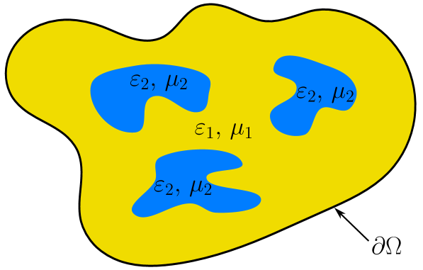
For the sake of simplicity, we consider here an electromagnetic medium (see 2 for an example) composed of two isotropic homogeneous materials which fills an open connected bounded Lipschitz domain $\Omega\subset{\mathbb{R}}^{3}$ (we refer to the Section 5.1 of [Kirsch and Hettlich 2015] for the definition of Lipschitz bounded domains which includes domains with nonsmooth boundary as polyhedra). However, our result could be easily extended to a medium composed of a finite number of anisotropic homogeneous materials, this is discussed in the last section. Thus, the dielectric permittivity $\varepsilon$ and the magnetic permeability $\mu$ which characterized this medium are supposed to be piecewise constant functions which take respectively the complex values $\varepsilon_{1}$ and $\mu_{1}$ in the first material, and $\varepsilon_{2}$ and $\mu_{2}$ in the second one. Moreover, we assume that both materials are passive, thus these functions have to satisfy (see [Milton 2002]; [Welters, Avniel, and Johnson 2014]; [Bernland, Luger, and Gustafsson 2011]; [Gustafsson and Sjöberg 2010]):

$$\operatorname{Im}(\omega\varepsilon)>0\,\mbox{ and }\,\operatorname{Im}(\omega\mu)>0\mbox{ for }\,\operatorname{Im}\omega>0,$$ (3.1)

where $\omega$ denotes the complex frequency.

The time-harmonic Maxwell’s equations (in Gaussian units) which link the electric and magnetic fields ${\bf E}$ and ${\bf H}$ in $\Omega$ are given by:

$$(\mathcal{P})\left\{\begin{array}[]{ll}\mathrm{curl\,}{\bf E}-i\omega\mu\,c^{-1}{\bf H}=0&\mbox{in }\Omega,\\[10.0pt] \mathrm{curl\,}{\bf H}+i\omega\varepsilon\,c^{-1}{\bf E}=0&\mbox{in }\Omega,\\[10.0pt] {\bf E}\times{\bf n}={\bf f}&\mbox{on }\partial\Omega.\end{array}\right.$$

where ${\bf n}$ denotes here the outward normal vector on the boundary of $\Omega$: $\partial\Omega$, $c$ the speed of light in the vacuum and ${\bf f}$ the tangential electric field ${\bf E}$ on $\partial\Omega$.

Figure 2: Example of the body $\Omega$.

Let us first introduce some classical functional spaces associated to the study of Maxwell’s equations:

• $L^{2}(\Omega)$ which is a Hilbert space endowed with the inner product:

  $$({\bf f},{\bf g})_{L^{2}(\Omega)}=\int_{\Omega}{\bf f}(x)\cdot\overline{{\bf g}(x)}\,\mathrm{d}{\bf x},$$

• $H(\mathrm{curl\,},\Omega)=\left\{{\bf u}\in L^{2}(\Omega)\,\mid\,\mathrm{curl\,}{\bf u}\in L^{2}(\Omega)\right\}$,

• $H_{0}(\mathrm{curl\,},\Omega)=\left\{{\bf u}\in H(\mathrm{curl\,},\Omega)\,\mid\,{\bf u}\times{\bf n}=0\mbox{ on }\partial\Omega\right\}$,

• $H^{-\frac{1}{2}}(\mathrm{div\,},\partial\Omega)=\left\{({\bf u}\times{\bf n})_{\partial\Omega}\,\mid\,{\bf u}\in H(\mathrm{curl\,},\Omega)\right\}$,

• $H^{-\frac{1}{2}}(\mathrm{curl\,},\partial\Omega)=\left\{{\bf n}\times({\bf u}\times{\bf n})_{\partial\Omega}\,\mid\,{\bf u}\in H(\mathrm{curl\,},\Omega)\right\}.$

Here $H(\mathrm{curl\,},\Omega)$ and $H_{0}(\mathrm{curl\,},\Omega)$ are Hilbert spaces endowed with the norm $\left\|\cdot\right\|_{H(\mathrm{curl\,},\Omega)}$ defined by

$$\left\|{\bf u}\right\|_{H(\mathrm{curl\,},\Omega)}^{2}=\left\|{\bf u}\right\|_{L^{2}(\Omega)}^{2}+\left\|\mathrm{curl\,}{\bf u}\right\|_{L^{2}(\Omega)}^{2}.$$

Concerning the functional framework associated with the spaces of tangential traces and tangential trace components $H^{-\frac{1}{2}}(\mathrm{div\,},\partial\Omega)$ and $H^{-\frac{1}{2}}(\mathrm{curl\,},\partial\Omega)$, we refer to the Section 5.1 of ?). These spaces are respectively Banach spaces for the norms $\|\cdot\|_{H^{-\frac{1}{2}}(\mathrm{curl\,},\partial\Omega)}$ and $\|\cdot\|_{H^{-\frac{1}{2}}(\mathrm{div\,},\partial\Omega)}$ introduced in the Definition 5.23 of ?) and are linked by the duality relation: $(H^{-\frac{1}{2}}(\mathrm{div\,},\partial\Omega))^{*}=H^{-\frac{1}{2}}(\mathrm{curl\,},\partial\Omega)$. Moreover, their duality product $\left\langle\cdot,\cdot\right\rangle$ (see Theorem 5.26 of ?)) satisfies the following Green’s identity:

$$\int_{\Omega}{\bf u}\cdot\mathrm{curl\,}{\bf v}-{\bf v}\cdot\mathrm{curl\,}{\bf u}\,\mathrm{d}{\bf x}=\left\langle{\bf n}\times({\bf v}\times{\bf n}),{\bf u}\times{\bf n}\right\rangle,\ \forall{\bf u},{\bf v}\in H(\mathrm{curl\,},\Omega).$$ (3.2)

Here we look for solutions $({\bf E},{\bf H})\in H(\mathrm{curl\,},\Omega)^{2}$ of the problem $(\mathcal{P})$ for data ${\bf f}\in H^{-\frac{1}{2}}(\mathrm{div\,},\partial\Omega)$.

3.2 The Dirichlet-to-Neumann map

We introduce the variable ${\bf Z}=(\omega\varepsilon_{1},\omega\varepsilon_{2},\omega\mu_{1},\omega\mu_{2})\in({\mathbb{C}}^{+})^{4}$. The electromagnetic Dirichlet-to-Neumann map $\Lambda_{{\bf Z}}:H^{-\frac{1}{2}}(\mathrm{div\,},\partial\Omega)\to H^{-\frac{1}{2}}(\mathrm{curl\,},\partial\Omega)$ associated to the problem $(\mathcal{P})$ is defined as the linear operator:

$$\Lambda_{{\bf Z}}\,{\bf f}=i\,{\bf n}\times({\bf H}\times{\bf n})_{\partial\Omega},\quad\forall{\bf f}\in H^{-\frac{1}{2}}(\mathrm{div\,},\partial\Omega).$$ (3.3)

Remark 16.

This definition of the DtN map (3.3) is slightly different from the one introduced in ?), ?) and ?). Here, the rotated tangential electric field ${\bf f}={\bf E}\times{\bf n}$ is mapped (up to a constant) to the tangential component of the magnetic field ${\bf n}\times({\bf H}\times{\bf n})=({\bf I}-{\bf n}{\bf n}^{T}){\bf H}$ and not to the rotated tangential magnetic field ${\bf H}\times{\bf n}$. This definition is closer to the one used in ?) to construct generalized impedance boundary conditions for electromagnetic scattering problems.

We want to prove the following theorem:

Theorem 17.

The DtN map $\Lambda_{{\bf Z}}$ is well-defined, is a continuous linear operator with respect to the datum ${\bf f}$ and is an analytic function of ${\bf Z}$ in the open set $({\mathbb{C}}^{+})^{4}$. Moreover, the operator $\Lambda_{{\bf Z}}$ satisfies

$$\operatorname{Im}\left\langle\Lambda_{{\bf Z}}\,{\bf f},\overline{{\bf f}}\right\rangle>0,\ \forall{\bf f}\in H^{-\frac{1}{2}}(\mathrm{div\,},\partial\Omega)-\{0\},$$ (3.4)

and as an immediate consequence, the function

$$h_{{\bf f}}({\bf Z})=\left\langle\Lambda_{{\bf Z}}\,{\bf f},\overline{{\bf f}}\right\rangle\mbox{ defined on }({\mathbb{C}}^{+})^{4}\mbox{ for all ${\bf f}\in H^{-\frac{1}{2}}(\mathrm{div\,},\partial\Omega)$}$$ (3.5)

is a Herglotz function of ${\bf Z}$ (see Definition 2).

Remark 18.

A similar theorem is obtained in the previous chapter of this book for a DtN map defined as the operator which maps the tangential electric field ${\bf n}\times({\bf E}\times{\bf n})$ to $i\,{\bf n}\times{\bf H}$ on $\partial\Omega$ . But for a regular boundary $\partial\Omega$ (for example $C^{1,1}$), this other definition of the DtN map can be rewritten as $-Q\Lambda_{{\bf Z}}\,Q$ with the isomorphism $Q:H^{-\frac{1}{2}}(\mathrm{curl\,},\partial\Omega)\to H^{-\frac{1}{2}}(\mathrm{div\,},\partial\Omega)$ defined by $Q({\bf g})=-{\bf n}\times{\bf g}$. Thus, one can show in the same way that the function

$$h_{{\bf g}}({\bf Z})=\left\langle\overline{{\bf g}},-Q\Lambda_{{\bf Z}}\,Q\,{\bf g}\right\rangle,\,\forall{\bf g}\in H^{-\frac{1}{2}}(\mathrm{curl\,},\partial\Omega)$$

is a Herglotz function on $({\mathbb{C}}^{+})^{4}$. But, as it is mentioned in Remark 1, p. 30 and Corollary 2, p. 38 of ?), the isomorphism $Q$ may not be well-defined if the function ${\bf n}$ is not regular enough. That is why, in order to make this connection, we assume that the boundary $\partial\Omega$ is slightly more regular than Lipschitz continuous.

3.3 Proof of the Theorem 17

We will first prove that the linear operator $T_{{\bf Z}}:H^{-\frac{1}{2}}(\mathrm{div\,},\partial\Omega)\to H(\mathrm{curl\,},\Omega)^{2}$ which associates the data ${\bf f}$ to the solution $({\bf E},{\bf H})\in H(\mathrm{curl\,},\Omega)^{2}$ of $(\mathcal{P})$ is well-defined, continuous and analytic in ${\bf Z}$ in $({\mathbb{C}}^{+})^{4}$. In other words that the problem $(\mathcal{P})$ admits a unique solution $({\bf E},{\bf H})$ which depends continuously on the data ${\bf f}$ and analytically on ${\bf Z}$. The approach we follow is standard, it uses a variational reformulation of the time-harmonic Maxwell’s equations $(\mathcal{P})$ (see [Cessenat 1996]; [Kirsch and Hettlich 2015]; [Monk 2003]; [Nedelec 2001]).

The first step is to introduce a lifting of the boundary data ${\bf f}$. As ${\bf f}\in H^{-\frac{1}{2}}(\mathrm{div\,},\partial\Omega)$, there exists (see Theorem 5.24 of [Kirsch and Hettlich 2015]) a continuous lifting operator $R:H^{-\frac{1}{2}}(\mathrm{div\,},\partial\Omega)\to H(\mathrm{curl\,},\Omega)$ such that

$$R({\bf f})={\bf E}_{0},$$ (3.6)

that is a field ${\bf E}_{0}\in H(\mathrm{curl\,},\Omega)$ which depends continuously on ${\bf f}$ such that ${\bf E}_{0}\times{\bf n}={\bf f}$ on $\partial\Omega$. Thus, the field $\tilde{{\bf E}}={\bf E}-{\bf E}_{0}$ satisfies the following problem with homogeneous boundary condition:

$$(\tilde{\mathcal{P}})\left\{\begin{array}[]{ll}\mathrm{curl\,}\tilde{{\bf E}}-i\omega\mu\,c^{-1}{\bf H}=-\mathrm{curl\,}{\bf E}_{0}&\mbox{in }\Omega,\\[10.0pt] \mathrm{curl\,}{\bf H}+i\omega\varepsilon\,c^{-1}\tilde{{\bf E}}=-i\omega\varepsilon\,c^{-1}{\bf E}_{0}&\mbox{in }\Omega,\\[10.0pt] \tilde{{\bf E}}\times{\bf n}=0&\mbox{on }\partial\Omega.\end{array}\right.$$

Now multiplying the second Maxwell’s equation of $(\tilde{\mathcal{P}})$ by a test function $\mbox{\boldmath${\psi}$}\in H_{0}(\mathrm{curl\,},\Omega)$, integrating by parts and then eliminating the unknown ${\bf H}$ by using the first Maxwell’s equation, we get the following variational formula for the electrical field $\tilde{{\bf E}}$:

$$\int_{\Omega}-c^{2}\,(\mu\omega)^{-1}\,\mathrm{curl\,}\tilde{{\bf E}}\cdot\overline{\mathrm{curl\,}\mbox{\boldmath${\psi}$}}+\omega\varepsilon\,\tilde{{\bf E}}\cdot\overline{\mbox{\boldmath${\psi}$}}\,\mathrm{d}{\bf x}=\int_{\Omega}c^{2}\,(\mu\omega)^{-1}\mathrm{curl\,}{\bf E}_{0}\cdot\overline{\mathrm{curl\,}\mbox{\boldmath${\psi}$}}-\omega\varepsilon\,{\bf E}_{0}\cdot\overline{\mbox{\boldmath${\psi}$}}\,\mathrm{d}{\bf x},$$ (3.7)

satisfied by all $\mbox{\boldmath${\psi}$}\in H_{0}(\mathrm{curl\,},\Omega)$. The variational formula (3.7) and the problem $(\mathcal{P})$ are equivalent.

Proposition 19.

$\tilde{{\bf E}}\in H_{0}(\mathrm{curl\,},\Omega)$ is a solution of the variational formulation (3.7) if and only if $\big{(}{\bf E}=\tilde{{\bf E}}+{\bf E}_{0},{\bf H}=c\,(i\mu\omega)^{-1}\mathrm{curl\,}(\tilde{{\bf E}}+{\bf E}_{0})\big{)}\in H(\mathrm{curl\,},\Omega)^{2}$ satisfy the problem $(\mathcal{P})$.

Proof.

This proof is standard. For more details, we refer to the demonstration of the lemma 4.29 in ?). ∎

For all ${\bf Z}\in({\mathbb{C}}^{+})^{4}$, we introduce the sesquilinear form:

$$a_{{\bf Z}}(\mbox{\boldmath${\phi}$},\mbox{\boldmath${\psi}$})=\int_{\Omega}-c^{2}(\mu\omega)^{-1}\,\mathrm{curl\,}\mbox{\boldmath${\phi}$}\cdot\overline{\mathrm{curl\,}\mbox{\boldmath${\psi}$}}+\omega\varepsilon\,\mbox{\boldmath${\phi}$}\cdot\overline{\mbox{\boldmath${\psi}$}}\,\mathrm{d}{\bf x},$$

defined on $H_{0}(\mathrm{curl\,},\Omega)^{2}$. One easily proves by using the Cauchy–Schwarz inequality that:

$$|a_{{\bf Z}}(\mbox{\boldmath${\phi}$},\mbox{\boldmath${\psi}$})|\leq\max\big{(}c^{2}\left\|(\omega\mu)^{-1}\right\|_{\infty},\left\|\omega\varepsilon\right\|_{\infty}\big{)}\,\left\|\mbox{\boldmath${\phi}$}\right\|_{H(\mathrm{curl\,},\Omega)}\,\left\|\mbox{\boldmath${\psi}$}\right\|_{H(\mathrm{curl\,},\Omega)},$$ (3.8)

where $\left\|\cdot\right\|_{\infty}$ denotes the $L^{\infty}$ norm. Thus, $a_{{\bf Z}}$ is continuous and as such it allows us to define a continuous linear operator $A_{{\bf Z}}\in L(H_{0}(\mathrm{curl\,},\Omega),H_{0}(\mathrm{curl\,},\Omega)^{*})$ by

$$\left\langle A_{{\bf Z}}\mbox{\boldmath${\phi}$},\mbox{\boldmath${\psi}$}\right\rangle_{H_{0}(\mathrm{curl\,},\Omega)}=a_{{\bf Z}}(\mbox{\boldmath${\phi}$},\overline{\mbox{\boldmath${\psi}$}}),\ \forall\mbox{\boldmath${\phi}$},\mbox{\boldmath${\psi}$}\in H_{0}(\mathrm{curl\,},\Omega),$$ (3.9)

where $\left\langle\cdot,\cdot\right\rangle_{H_{0}(\mathrm{curl\,},\Omega)}$ stands for the duality product between $H_{0}(\mathrm{curl\,},\Omega)$ and its dual $H_{0}(\mathrm{curl\,},\Omega)^{*}$. We now introduce the antilinear form $l_{{\bf Z}}({\bf E}_{0})(\cdot)$:

$$l_{{\bf Z}}({\bf E}_{0})(\mbox{\boldmath${\psi}$})=\int_{\Omega}c^{2}\,(\mu\omega)^{-1}\mathrm{curl\,}{\bf E}_{0}\cdot\overline{\mathrm{curl\,}\mbox{\boldmath${\psi}$}}-\omega\varepsilon\,{\bf E}_{0}\cdot\overline{\mbox{\boldmath${\psi}$}}\,\mathrm{d}{\bf x},\,\forall\mbox{\boldmath${\psi}$}\in H_{0}(\mathrm{curl\,},\Omega).$$

In the same way as (3.8), one can easily check:

$$|l_{{\bf Z}}({\bf E}_{0})(\mbox{\boldmath${\psi}$})|\leq\max\big{(}c^{2}\,\left\|(\omega\mu)^{-1}\right\|_{\infty},\left\|\omega\varepsilon\right\|_{\infty}\big{)}\,\left\|{\bf E}_{0}\right\|_{H(\mathrm{curl\,},\Omega)}\,\left\|\mbox{\boldmath${\psi}$}\right\|_{H(\mathrm{curl\,},\Omega)}.$$

Hence, the linear operator $L_{{\bf Z}}:H(\mathrm{curl\,},\Omega)\to H_{0}(\mathrm{curl\,},\Omega)^{*}$ defined by

$$\left\langle L_{{\bf Z}}{\bf E}_{0},\mbox{\boldmath${\psi}$}\right\rangle_{H_{0}(\mathrm{curl\,},\Omega)}=l_{{\bf Z}}({\bf E}_{0})(\overline{\mbox{\boldmath${\psi}$}}),\ \forall{\bf E}_{0}\in H(\mathrm{curl\,},\Omega)\mbox{ and }\forall\,\mbox{\boldmath${\psi}$}\in H_{0}(\mathrm{curl\,},\Omega),$$ (3.10)

is well-defined and continuous. Thus, we deduce from the relations (3.8) and (3.10) that the variational formula (3.7) is equivalent to solve the following infinite dimensional linear system

$$A_{{\bf Z}}\,\tilde{{\bf E}}=L_{{\bf Z}}\,{\bf E}_{0}.$$ (3.11)

Proposition 20.

If ${\bf Z}\in({\mathbb{C}}^{+})^{4}$, then the operator $A_{{\bf Z}}$ is an isomorphism from $H_{0}(\mathrm{curl\,},\Omega)$ to $H_{0}(\mathrm{curl\,},\Omega)^{*}$ and its inverse $A_{{\bf Z}}^{-1}$ depends analytically on ${\bf Z}$ in $({\mathbb{C}}^{+})^{4}$.

Proof.

Let ${\bf Z}$ be in $({\mathbb{C}}^{+})^{4}$. The invertibility of $A_{{\bf Z}}$ is an immediate consequence of the Lax–Milgram Theorem. Indeed, the coercivity of the sesquilinear form $a_{{\bf Z}}$ derives from the passivity hypothesis (3.1) of the material:

$$|a_{{\bf Z}}(\mbox{\boldmath${\phi}$},\mbox{\boldmath${\phi}$})|\geq\operatorname{Im}\big{(}a_{{\bf Z}}(\mbox{\boldmath${\phi}$},\mbox{\boldmath${\phi}$})\big{)}\geq\alpha\left\|\mbox{\boldmath${\phi}$}\right\|_{H(\mathrm{curl\,},\Omega)}^{2},\ \forall\mbox{\boldmath${\phi}$}\in H_{0}(\mathrm{curl\,},\Omega),$$

where $\alpha=\min\big{(}\operatorname{Im}(\omega\varepsilon_{1}),\operatorname{Im}(\omega\varepsilon_{2}),-c^{2}\operatorname{Im}(\,(\omega\mu_{1})^{-1}),-c^{2}\operatorname{Im}(\omega\mu_{2})^{-1})\big{)}>0$.

Now the analyticity in ${\bf Z}$ of the operator $A_{{\bf Z}}^{-1}$ is proved as follows. First, one can verify easily that for all $\mbox{\boldmath${\phi}$},{\psi}\in H_{0}(\mathrm{curl\,},\Omega)$, the sesquilinear form $a_{{\bf Z}}(\mbox{\boldmath${\phi}$},\overline{{\psi}})$ depends analytically on each component of ${\bf Z}$ when the others are fixed. It follows immediately from this and Theorem 6 that the operator $A_{{\bf Z}}$ [defined by the relation (3.9)] is analytic in the operator norm of $L(H_{0}(\mathrm{curl\,},\Omega),H_{0}(\mathrm{curl\,},\Omega)^{*})$ and hence by Theorem 4 (Hartogs’ Theorem) it is analytic in ${\bf Z}$ in the open set $({\mathbb{C}}^{+})^{4}$. Thus, since $A_{{\bf Z}}$ is an isomorphism which depends analytically on ${\bf Z}$ in the open set $({\mathbb{C}}^{+})^{4}$, then by Theorem 5 its inverse $A_{{\bf Z}}^{-1}$ depends analytically on ${\bf Z}$ in $({\mathbb{C}}^{+})^{4}$. ∎

Using Theorem 4 again, one can easily check in the same way as for the operator $A_{{\bf Z}}$ that the operator $L_{{\bf Z}}$ defined by (3.10) is also analytic in ${\bf Z}$ in $({\mathbb{C}}^{+})^{4}$. Hence, the variational formula $(\ref{Feq.var})$ admits a unique solution:

$$\tilde{{\bf E}}=A_{{\bf Z}}^{-1}L_{{\bf Z}}\,{\bf E}_{0}=A_{{\bf Z}}^{-1}L_{{\bf Z}}\,R({\bf f})$$ (3.12)

which depends continuously on the data ${\bf f}$ and analytically on ${\bf Z}$ in $({\mathbb{C}}^{+})^{4}$.

Corollary 21.

The linear operator $T_{{\bf Z}}:H^{-\frac{1}{2}}(\mathrm{div\,},\partial\Omega)\to H(\mathrm{curl\,},\Omega)^{2}$ which maps the data ${\bf f}$ to the solution $({\bf E},{\bf H})\in H(\mathrm{curl\,},\Omega)^{2}$ of $(\mathcal{P})$ is well-defined, continuous and depends analytically on ${\bf Z}$ in $({\mathbb{C}}^{+})^{4}$.

Proof.

This result is just a consequence of Propositions 19 and 20 which prove that the time-harmonic Maxwell’s equations $(\mathcal{P})$ admits a unique solution $({\bf E},{\bf H})=T_{{\bf Z}}({\bf f})\in H(\mathrm{curl\,},\Omega)^{2}$ for data ${\bf f}\in H^{-\frac{1}{2}}(\mathrm{div\,},\partial\Omega)$ where the linear operator $T_{{\bf Z}}$ is defined by the following relation:

$$T_{{\bf Z}}({\bf f})=\big{(}R({\bf f})+\tilde{{\bf E}},c\,(i\mu\omega)^{-1}\mathrm{curl\,}(\tilde{{\bf E}}+R({\bf f})\big{)},\ \forall{\bf f}\in H^{-\frac{1}{2}}(\mathrm{div\,},\partial\Omega),$$ (3.13)

where $\tilde{{\bf E}}=A_{{\bf Z}}^{-1}L_{{\bf Z}}\,R({\bf f})$ by the relation (3.12) and $R$ stands for the lifting operator defined in (3.6). With the relation (3.13), the continuity of $T_{{\bf Z}}$ with respect to ${\bf f}$ and its analyticity with respect to ${\bf Z}$ follow immediately from the corresponding properties of the operator $A_{{\bf Z}}^{-1}$, $L_{{\bf Z}}$ and $R$. ∎

We now introduce the tangential component trace operator $\gamma_{T}:H(\mathrm{curl\,},\Omega)\to H^{-\frac{1}{2}}(\mathrm{curl\,},\partial\Omega)$ defined by:

$$\gamma_{T}({\bf H})={\bf n}\times({\bf H}\times{\bf n})_{\partial\Omega},\ \forall{\bf H}\in H(\mathrm{curl\,},\Omega),$$ (3.14)

which is continuous (see Theorem 5.24 of [Kirsch and Hettlich 2015]) and the continuous linear operator $P:H(\mathrm{curl\,},\Omega)^{2}\to H(\mathrm{curl\,},\Omega)$ defined by:

$$P({\bf E},{\bf H})={\bf H},\ \forall{\bf E},{\bf H}\in H(\mathrm{curl\,},\Omega).$$ (3.15)

This gives us the following operator representation of the electromagnetic DtN map defined in (3.3).

Proposition 22.

(Electromagnetic Dirichlet-to-Neumann map) The electromagnetic DtN map $\Lambda_{{\bf Z}}:H^{-\frac{1}{2}}(\mathrm{div\,},\partial\Omega)\to H^{-\frac{1}{2}}(\mathrm{curl\,},\partial\Omega)$ is the continuous linear operator defined by the composition of the continuous linear operators $\gamma_{T}$ in (3.14), $P$ in (3.15) and $T_{{\bf Z}}$ in (3.13) by

$$\Lambda_{{\bf Z}}({\bf f})=i\,\gamma_{T}\,P\,T_{{\bf Z}}({\bf f}),\ \forall{\bf f}\in H^{-\frac{1}{2}}(\mathrm{div\,},\partial\Omega).$$ (3.16)

Proof.

Let ${\bf f}\in H^{-\frac{1}{2}}(\mathrm{div\,},\partial\Omega)$. Then $({\bf E},{\bf H})=T_{{\bf Z}}({\bf f})$ is the solution of problem ($\mathcal{P}$). Thus, by definition of $\gamma_{T}$ and $P$ we have $PT_{{\bf Z}}({\bf f})={\bf H}$ and hence $i\gamma_{T}PT_{{\bf Z}}({\bf f})=i{\bf n}\times({\bf H}\times{\bf n})_{\partial\Omega}$. Therefore, by the definition (3.3) of the DtN map we have $\Lambda_{{\bf Z}}({\bf f})=i\gamma_{T}PT_{{\bf Z}}({\bf f})$. The fact that $\Lambda_{{\bf Z}}$ is a continuous linear operator follows immediately from this representation. This completes the proof. ∎

We can now derive the regularity properties of the DtN map $\Lambda_{{\bf Z}}$ by expressing this operator in terms of the operator $T_{{\bf Z}}$. The analyticity of the DtN map $\Lambda_{{\bf Z}}$ with respect to ${\bf Z}$ in $({\mathbb{C}}^{+})^{4}$ is now an immediate consequence of the fact that $\Lambda_{{\bf Z}}$ is the composition of two continuous linear operators $i\,\gamma_{T}$ and $P$ independent of ${\bf Z}$ with the continuous linear operator $T_{{\bf Z}}$ which is analytic in ${\bf Z}$ (see Corollary 21).

Finally, to prove the positivity of $\operatorname{Im}\left\langle\Lambda_{{\bf Z}}{\bf f},\overline{{\bf f}}\right\rangle$, we apply Green’s identity (3.2) to the solution $({\bf E},{\bf H})$ of the problem $(\mathcal{P})$ for any nonzero data ${\bf f}\in H^{-\frac{1}{2}}(\mathrm{div\,},\partial\Omega)$. It yields

$$i\int_{\Omega}\overline{{\bf E}}\cdot\mathrm{curl\,}{\bf H}-{\bf H}\cdot\overline{\mathrm{curl\,}{\bf E}}\,\mathrm{d}\Omega=i\left\langle{\bf n}\times({\bf H}\times{\bf n}),\overline{{\bf E}}\times{\bf n}\right\rangle=\left\langle\Lambda_{{\bf Z}}\,{\bf f},\overline{{\bf f}}\right\rangle.$$

Since $({\bf E},{\bf H})$ is a solution of the time-harmonic Maxwell equations $(\mathcal{P})$, we can rewrite this last relation as:

$$\int_{\Omega}\omega\varepsilon\,c^{-1}\left|{\bf E}\right|^{2}-\overline{\omega\mu}\,c^{-1}\left|{\bf H}\right|^{2}\mathrm{d}{\bf x}=\left\langle\Lambda_{{\bf Z}}\,{\bf f},\overline{{\bf f}}\right\rangle.$$ (3.17)

By taking the imaginary part of (3.17) and using the passivity hypothesis (3.1) of the materials which compose the medium $\Omega$, we get the positivity of $\operatorname{Im}\left\langle\Lambda_{{\bf Z}}{\bf f},\overline{{\bf f}}\right\rangle$ (3.4) (since $({\bf E},{\bf H})\neq(0,0)$ for ${\bf f}\neq 0$) and it follows immediately that the function $h_{{\bf f}}$ defined by (3.5) is a Herglotz function of ${\bf Z}$.

3.4 Extensions of Theorem 17 to anisotropic and continuous media

Here we first extend Theorem 17 to the case of a medium $\Omega$ composed by $N$ anisotropic homogeneous phases. Therefore, the dielectric permittivity $\mbox{\boldmath${\varepsilon}$}({\bf x})$ and magnetic permeability $\mbox{\boldmath${\mu}$}({\bf x})$ are now $3\times 3$ tensor-valued functions of ${\bf x}$, which take for $j=1,\cdots,N$ the constant values $\mbox{\boldmath${\varepsilon}$}_{j}$ and $\mbox{\boldmath${\mu}$}_{j}$ in the $j$th material. Again, each material is supposed to be passive, in the sense that $\operatorname{Im}(\omega\mbox{\boldmath${\varepsilon}$}_{j})$ and $\operatorname{Im}(\omega\mbox{\boldmath${\mu}$}_{j})$ have to be positive tensors for all $j=1,\cdots,N$ (see [Milton 2002], [Welters, Avniel, and Johnson 2014], [Bernland, Luger, and Gustafsson 2011], [Gustafsson and Sjöberg 2010]).

First, we want to emphasize that besides the fact that ${\varepsilon}$ and ${\mu}$ are now tensor-valued, the time-harmonic Maxwell’s equations $(\mathcal{P})$ in $\Omega$ and its associated functional spaces remain the same. Moreover, as the vector space $M_{3}({\mathbb{C}})$ is isomorphic to ${\mathbb{C}}^{9}$, we prove exactly in the same way that the DtN map $\Lambda_{{\bf Z}}$ defined by (3.3) is well-defined, is linear continuous with respect to ${\bf f}$, and is an analytic function with respect to ${\bf Z}$, where ${\bf Z}$ is here the vector of the $18N$ coefficients which are the elements (in some basis) of the tensors $\omega\mbox{\boldmath${\varepsilon}$}_{j}$ and $\omega\mbox{\boldmath${\mu}$}_{j}$ for $j=1,\cdots,N$, in the open set $\mathcal{O}$ of ${\mathbb{C}}^{18N}$ characterized by the passivity relation (3.1). As $\mathcal{O}$ is isomorphic to the open set $(M_{3}^{+}(\mathbb{C}))^{2N}$, this is equivalent to say (as it is explained in the last paragraph of the subsection 2.2) that $\Lambda_{{\bf Z}}$ is an analytic function of the vector ${\bf Z}$, whose components are now those of the permittivity tensors $\omega\mbox{\boldmath${\varepsilon}$}_{j}$ and permeability $\omega\mbox{\boldmath${\mu}$}_{j}$ (for $j=1,\cdots,N$) in each phase. Using the passivity assumption which is associated with the elements of $(M_{3}^{+}(\mathbb{C}))^{2N}$, one proves also identically the relation (3.4) on the DtN map for all ${\bf Z}\in(M_{3}^{+}(\mathbb{C}))^{2N}$.

The problem is now to define the notion of a Herglotz function. Indeed, when the tensors $\mbox{\boldmath${\varepsilon}$}_{j}$ and $\mbox{\boldmath${\mu}$}_{j}$ of each composite are not all diagonal, it is not possible anymore to define the DtN map as a multivariate Herglotz function $h_{{\bf f}}$ on some copy of the upper-half plane: $(\mathbb{C}^{+})^{n}$. The major obstruction to this construction is based on the simple observation that off-diagonal elements of a matrix in $M_{3}^{+}(\mathbb{C})$ will not necessarily have a positive imaginary part. Nevertheless, it is natural to define a Herglotz function which maps points ${\bf Z}$ represented by a $2N$-tuple of matrices ${\bf L}_{1}^{\prime},{\bf L}_{2}^{\prime},\ldots{\bf L}_{2N}^{\prime}$ with positive definite imaginary parts, i.e., ${\bf Z}=({\bf L}_{1}^{\prime},{\bf L}_{2}^{\prime},\ldots{\bf L}_{2N}^{\prime})$, to the upper half-plane.

One way to preserve the Herglotz property is to use a trajectory method (see [Bergman 1978] and Section 18.6 of [Milton 2002]), in other words, consider an analytic function $s\mapsto{\bf Z}(s)$ from ${\mathbb{C}}^{+}$ into $(M_{3}^{+}(\mathbb{C}))^{2N}$, i.e., a trajectory in one complex dimension (a surface in two real directions). Then, along this trajectory, we obtain immediately that the function

$$h_{{\bf f}}(s)=\,\left\langle\Lambda_{{\bf Z}(s)}{\bf f},\overline{{\bf f}}\right\rangle,\ \forall{\bf f}\in H^{-\frac{1}{2}}(\mathrm{div\,},\partial\Omega),$$ (3.18)

is a Herglotz function (see Definition 2) of $s$ in ${\mathbb{C}}^{+}$: analyticity follows from the fact that analyticity is preserved under composition of analytic functions, while, when $s$ has positive imaginary part, nonnegativity of the imaginary part of $h_{{\bf f}}(s)$ follows from the fact that ${\bf Z}(s)$ lies in the domain where the imaginary part of the operator $\Lambda_{{\bf Z}(s)}$ is positive semi-definite.

A particularly interesting trajectory for electromagnetism, in an $N$-phase material, is the trajectory

$$s=\omega\to{\bf Z}(\omega)=(\omega\mbox{\boldmath${\varepsilon}$}_{1}(\omega),\omega\mbox{\boldmath${\varepsilon}$}_{2}(\omega),\ldots,\omega\mbox{\boldmath${\varepsilon}$}_{N}(\omega),\omega\mbox{\boldmath${\mu}$}_{1}(\omega),\omega\mbox{\boldmath${\mu}$}_{2}(\omega),\ldots,\omega\mbox{\boldmath${\mu}$}_{N}(\omega)),$$

where $\mbox{\boldmath${\varepsilon}$}_{j}(\omega)$ and $\mbox{\boldmath${\mu}$}_{j}(\omega)$ are the physical electric permittivity tensor and physical magnetic permeability tensor of the actual material constituting phase $i$ as functions of the frequency $\omega$. Due to the passive nature of these materials the trajectory maps $\omega$ in the upper half plane ${\mathbb{C}}^{+}$ into a trajectory in $(M_{3}^{+}(\mathbb{C}))^{2N}$ . The physical interest about this trajectory is that one can in principle measure $\Lambda_{{\bf Z}(\omega)}$ along it, at least for real frequencies $\omega$.

In the case of the trajectory method, one can easily generalize Theorem 17 to continuous anisotropic composites where ${\varepsilon}$ and ${\mu}$ are matrix-valued functions of both variables $({\bf x},\omega)\in\Omega\times{\mathbb{C}}^{+}$. In this case, we suppose that

• (H1) For all $\omega\in{\mathbb{C}}^{+}$, $\mbox{\boldmath${\varepsilon}$}(\cdot,\omega)$ and $\mbox{\boldmath${\mu}$}(\cdot,\omega)$ are $L^{\infty}$ matrix-valued functions on $\Omega$ which are locally bounded in the variable $\omega$, in other words, we suppose that there exists $\delta>0$ such that the open ball of center $\omega$ and radius $\delta$: $B(\omega,\delta)$ is included in ${\mathbb{C}}^{+}$ and that

  $$\sup_{z\in B(\omega,\delta)}\|\mbox{\boldmath${\varepsilon}$}(\cdot,z)\|_{\infty}<\infty\mbox{ and }\sup_{z\in B(\omega,\delta)}\|\mbox{\boldmath${\mu}$}(\cdot,z)\|_{\infty}<\infty$$ (3.19)

• (H2) The composite is passive which implies that for almost every $x\in\Omega$, the functions $\omega\mapsto\omega\mbox{\boldmath${\varepsilon}$}({\bf x},\omega)$ and $\omega\mapsto\omega\mbox{\boldmath${\mu}$}({\bf x},\omega)$ are analytic functions from ${\mathbb{C}}^{+}$ to $M_{3}^{+}(\mathbb{C})$ (see Section 11.1 of [Milton 2002]).

• (H3) For all $\omega\in{\mathbb{C}}^{+}$, there exists $C_{\omega}>0$ such that

  $$\operatorname{ess}\inf\limits_{{\bf x}\in\Omega}\operatorname{Im}(\omega\mbox{\boldmath${\varepsilon}$}(\cdot,\omega))\geq C_{\omega}\operatorname{Id}\ \mbox{ and }\ \operatorname{ess}\inf\limits_{{\bf x}\in\Omega}-(\operatorname{Im}(\omega\mbox{\boldmath${\mu}$}(\cdot,\omega))^{-1}\geq C_{\omega}\operatorname{Id}.$$ (3.20)

Remark 23.

The hypotheses (H1) and (H3) may seem complicated but they are satisfied for instance when ${\varepsilon}$ and ${\mu}$ are continuous functions of both variables $({\bf x},\omega)\in\operatorname{cl}\Omega\times\mathbb{C}^{+}$, where $\operatorname{cl}\Omega$ denotes the closure of $\Omega$. In that case, one can see immediately that $(H1)$ is satisfied. Moreover, if we assume also that the passivity assumption (H2) holds on $\operatorname{cl}\Omega$ (instead of just $\Omega$), the hypothesis (H3) is also satisfied since the functions $\operatorname{Im}(\omega\mbox{\boldmath${\varepsilon}$}(\cdot,\omega))$ and $-(\operatorname{Im}(\omega\mbox{\boldmath${\mu}$}(\cdot,\omega)))^{-1}$ are continuous functions on a compact set and thus reach their minimum value which is a positive matrix.

Under these hypotheses, Theorem 17 remains valid: the function $h_{{\bf f}}(\omega)$ given by (3.5) is a Herglotz function of the frequency (by interpreting each formula of Section 3 with ${\bf Z}=\omega\in\mathbb{C}^{+}$ as a new analytic variable and ${\varepsilon}$ and ${\mu}$ as matrix valued functions of the variables $({\bf x},\omega)$). Moreover, the proof is basically the same as the one in Subsection 3.3. We just make precise here the justification of some technical points which appear when one reproduces this proof in this framework.

We first remark that the assumption (H1) on the tensors ${\varepsilon}$ and ${\mu}$ implies that the tensors $\omega\mbox{\boldmath${\varepsilon}$}(\cdot,\omega)$ and $(\omega\mbox{\boldmath${\mu}$}(\cdot,\omega))^{-1}$ are bounded functions of the space variable ${\bf x}$. Thus the bilinear form $a_{\omega}$ remains continuous and the operators $A_{\omega}$ and $L_{\omega}$ are still well-defined and continuous. With the coercivity hypothesis (H3), one can easily check that $\forall\mbox{\boldmath${\phi}$}\in H_{0}(\mathrm{curl\,},\Omega),$

$$|a_{\omega}(\mbox{\boldmath${\phi}$},\mbox{\boldmath${\phi}$})|\geq C_{\omega}\left\|\mbox{\boldmath${\phi}$}\right\|_{H(\mathrm{curl\,},\Omega)}^{2},$$

and apply again the Lax–Milgram theorem to show the invertibility of $A_{\omega}$. Then, the analyticity of the operators $A_{\omega}$ and $L_{\omega}$ with respect to $\omega$ in ${\mathbb{C}}^{+}$ is still obtained (thanks to the relations (3.9) and (3.10)) from their weak analyticity (see Theorem 6). This weak analyticity is proved by using Theorem 7 to show the analyticity of the integrals which appear in the expression of $\left\langle A_{\omega}\mbox{\boldmath${\phi}$},\mbox{\boldmath${\psi}$}\right\rangle_{H_{0}(\mathrm{curl\,},\Omega)}$ and $\left\langle L_{\omega}{\bf E}_{0},\mbox{\boldmath${\psi}$}\right\rangle_{H_{0}(\mathrm{curl\,},\Omega)}$ for ${\phi}$, ${\psi}\in H_{0}(\mathrm{curl\,},\Omega)$ and ${\bf E}_{0}\in H(\mathrm{curl\,},\Omega)$ (since the assumptions (H1) and (H2) imply the hypotheses of Theorem 7). Then the analyticity of $A_{\omega}^{-1}$ is proved by using again Theorem 5 and the rest of the proof follows by the same arguments as in the isotropic case.

4 Herglotz functions associated with anisotropic media

A theory of Herglotz functions directly defined on tensors and not only on scalar variables is particularly useful in the domain of bodies containing anisotropic materials such as, for instance, sea ice (see [Carsey 1992, Stogryn 1987, Golden 1995, Golden 2009, Gully, Lin, Cherkaev, and Golden 2015]) or in electromagnetism where it will even extend to complicated media such as gyrotropic materials for which the dielectric tensors and magnetic tensors are anisotropic but not symmetric (as there is no reciprocity principle in such media, see [Landau, Lifshitz, and Pitaevskiĭ 1984]). The idea for Herglotz representations of the effective moduli of anisotropic materials was first put forward in the appendix E of ?), and was studied in depth in Chapter 18 of ?), see also ?). In connection with sea ice, one is particularly interested in bounds where the moduli are complex: such bounds are an immediate corollary of appendix E of ?) and series expansions of the effective conductivity ([Willemse and Caspers 1979]; [Avellaneda and Bruno 1990]) that are contingent on assumptions about the polycrystalline geometry, and more generally are obtained (even for viscoelasticity with anisotropic phases) in ?) (to make the connection, see the discussion in Section 15 of the companion paper [Milton 1987a]), and also see the bounds (16.45) in ?). Explicit calculations were made by ?) and are in good agreement with sea ice measurements.

The trajectory method provides the desired representation, as shown in Section 18.8 of ?). We slightly modify that argument here. Given any tensors ${\bf L}_{j}=\omega\mbox{\boldmath${\varepsilon}$}_{j}$ and ${\bf L}_{j+N}=\omega\mbox{\boldmath${\mu}$}_{j}$, for $j=1,2,\ldots N$, which we assume to have strictly positive definite imaginary parts, and given a reference tensor ${\bf L}_{0}$ which is real, but not necessarily positive definite, define the real matrices

$${\bf A}_{j}=\mathop{\rm Re}\nolimits[({\bf L}_{0}-{\bf L}_{j})^{-1}],\quad{\bf B}_{j}=\mathop{\rm Im}\nolimits[({\bf L}_{0}-{\bf L}_{j})^{-1}],\quad j=1,2,\ldots,2N,$$ (4.21)

where, according to our assumption, ${\bf B}_{j}$ is positive definite for each $j$. Then consider the trajectory

$${\bf Z}(s)=({\bf L}_{1}^{\prime}(s),{\bf L}_{2}^{\prime}(s),\ldots{\bf L}_{2N}^{\prime}(s)),\quad{\rm where}\,\,{\bf L}_{j}^{\prime}(s)={\bf L}_{0}-({\bf A}_{j}+s{\bf B}_{j})^{-1}.$$ (4.22)

Each of the matrices ${\bf L}_{j}^{\prime}(s)$ have positive definite imaginary parts when $s$ is in $\mathbb{C}^{+}$, and so ${\bf Z}(s)$ maps $\mathbb{C}^{+}$ to $(M_{3}^{+}(\mathbb{C}))^{2N}$. Furthermore, by construction our trajectory passes through the desired point at $s=i$:

$${\bf Z}(i)=(\omega\mbox{\boldmath${\varepsilon}$}_{1},\omega\mbox{\boldmath${\varepsilon}$}_{2},\ldots,\omega\mbox{\boldmath${\varepsilon}$}_{N},\omega\mbox{\boldmath${\mu}$}_{1},\omega\mbox{\boldmath${\mu}$}_{2},\ldots\omega\mbox{\boldmath${\mu}$}_{N}).$$ (4.23)

Now $\Lambda_{{\bf Z}(s)}$ is an operator valued Herglotz function of $s$, and so has an integral representation involving a positive semi-definite operator-valued measure deriving from the values that ${\bf Z}(s)$ takes when $s$ is just above the positive real axis. That measure in turn is linearly dependent on the measure derived from the values that $\Lambda_{{\bf Z}({\bf L}_{1}^{\prime},{\bf L}_{2}^{\prime},\ldots{\bf L}_{2N}^{\prime})}$ takes as imaginary parts of ${\bf L}_{j}^{\prime}$ become vanishingly small. Thus ${\bf Z}(i)$ can be expressed directly in terms of this latter measure, involving an integral kernel ${\bf K}_{{\bf L}_{0}}({\bf L}_{1},{\bf L}_{2},\ldots{\bf L}_{2N},{\bf L}_{1}^{\prime},{\bf L}_{2}^{\prime},\ldots{\bf L}_{2N}^{\prime})$ that is singular with support that is concentrated on the trajectory which is traced by $({\bf L}_{1}^{\prime}(s),{\bf L}_{2}^{\prime}(s),\ldots{\bf L}_{2N}^{\prime}(s))$ as $s$ is varied along the real axis. The formula for $\Lambda_{{\bf Z}(i)}$ obtained from the above prescription can be rewritten (informally) as

$$\Lambda_{{\bf Z}({\bf L}_{1},{\bf L}_{2},\ldots{\bf L}_{2N})}=\int{\bf K}_{{\bf L}_{0}}({\bf L}_{1},{\bf L}_{2},\ldots{\bf L}_{2N},{\bf L}_{1}^{\prime},{\bf L}_{2}^{\prime},\ldots{\bf L}_{2N}^{\prime})\,d{\bf m}({\bf L}_{1}^{\prime},{\bf L}_{2}^{\prime},\ldots{\bf L}_{2N}^{\prime}).$$ (4.24)

An explicit formula could be obtained for the kernel ${\bf K}_{{\bf L}_{0}}({\bf L}_{1},{\bf L}_{2},\ldots{\bf L}_{2N},{\bf L}_{1}^{\prime},{\bf L}_{2}^{\prime},\ldots{\bf L}_{2N}^{\prime})$, which is non-zero except on the path traced out by $({\bf L}_{1}^{\prime}(s),{\bf L}_{2}^{\prime}(s),\ldots{\bf L}_{2N}^{\prime}(s))$ as $s$ varies over the reals, and this path depends on ${\bf L}_{0}$ and the moduli of ${\bf L}_{1},{\bf L}_{2},\ldots{\bf L}_{2N}$. The measure $d{\bf m}({\bf L}_{1}^{\prime},{\bf L}_{2}^{\prime},\ldots{\bf L}_{2N}^{\prime})$ is derived from the values that $\Lambda_{{\bf Z}({\bf L}_{1}^{\prime},{\bf L}_{2}^{\prime},\ldots{\bf L}_{2N}^{\prime})}$ takes as imaginary parts of ${\bf L}_{j}^{\prime}$ become vanishingly small.

The trajectory method has been unjustly criticised for failing to separate the dependence of the function (in this case $\Lambda_{{\bf Z}({\bf L}_{1},{\bf L}_{2},\ldots{\bf L}_{2N})}$) on the moduli (in this case the tensors ${\bf L}_{1},{\bf L}_{2},\ldots{\bf L}_{2N}$) from the dependence on the geometry, which is contained in the measure (in this case derived from the values that $\Lambda_{{\bf Z}({\bf L}_{1}^{\prime},{\bf L}_{2}^{\prime},\ldots{\bf L}_{2N}^{\prime})}$ takes as imaginary parts of ${\bf L}_{j}^{\prime}$ become vanishingly small.) But we see that (4.24) makes such a separation.

Now there are differences between this representation and standard representation formulas for multivariate Herglotz functions, but the main difference is that the kernel ${\bf K}_{{\bf L}_{0}}({\bf L}_{1},{\bf L}_{2},\ldots{\bf L}_{2N},{\bf L}_{1}^{\prime},{\bf L}_{2}^{\prime},\ldots{\bf L}_{2N}^{\prime})$, unlike the Szegő kernel which enters the polydisk representation of ?), is singular, being concentrated on this trajectory. However, for each choice of ${\bf L}_{0}$ there is a representation, each involving a kernel with support on a different trajectory and so one can average the representations over the matrices ${\bf L}_{0}$ with any desired smooth nonnegative weighting, to obtain a family of representations with less singular kernels that are the average over ${\bf L}_{0}$ of ${\bf K}_{{\bf L}_{0}}({\bf L}_{1},{\bf L}_{2},\ldots{\bf L}_{2N},{\bf L}_{1}^{\prime},{\bf L}_{2}^{\prime},\ldots{\bf L}_{2N}^{\prime})$. This nonuniqueness in the choice of kernel reflects the fact that the measure satisfies certain Fourier constraints on the polydisk (see ?)).

Another approach to considering of the notion of Herglotz functions in anisotropic multicomponent media is as follows. It will consist of proving that $(M_{3}^{+}(\mathbb{C}))^{2N}$ is isometrically isomorphic to a tubular domain (defined below) of $\mathbb{C}^{18N}$ and use it to extend the definition of Herglotz functions via the theory of holomorphic functions on tubular domains with nonnegative imaginary part from [Vladimirov 2002].

As we have already mentioned in the introduction to this chapter and at the end of Subsection 3.4, this extended definition is significant because these multivariate functions provide a deep connection to the theory of multivariate passive linear systems as described in Section 20 of [Vladimirov 2002], for instance, and in the study of anisotropic composites (e.g., sea ice or gyrotropic media). In addition to this, such an extension may allow for a more general approach of the efforts of ?) and ?) to derive integral representations of multivariate Herglotz functions in $({\mathbb{C}}^{+})^{N}$, beyond that provided in Section 18.8 of ?), or for deriving bounds in the theory of composites using the analytic continuation method (see Chapter 27 in [Milton 2002]).

Let us first introduce the definition of a tubular domain from Chapter 2, Section 9 of [Vladimirov 2002].

Definition 24.

Let $\Gamma$ be a closed convex acute cone in ${\mathbb{R}}^{N}$ with vertex at ${\bf 0}$. We denote by $C=\operatorname{int}(\Gamma^{*})$, where $\Gamma^{*}$ stands for the dual of $C$ (in the sense of cones’ duality) and $\operatorname{int}(\Gamma^{*})$ denotes the (topological) interior of $\Gamma^{*}$. Thus, $C$ is an open, convex, nonempty cone. Then, a tubular domain in $\mathbb{C}^{N}$ with base $C$ is defined as:

$$\mathcal{T}={\mathbb{R}}^{N}+iC=\left\{{\bf z}={\bf x}+i{\bf y}|{\bf x}\in{\mathbb{R}}^{N}\mbox{ and }{\bf y}\in C\right\}.$$

We will now show that $M_{N}^{+}({\mathbb{C}})$ is isometrically isomorphic to a tubular domain $\mathcal{T}^{C}$ of ${\mathbb{C}}^{N^{2}}$ [see Proposition 25, Proposition 26, and Theorem 27 below (which we state without proof as they are easily verified)]. Toward this purpose, we first use the decomposition

$${\bf M}=\frac{{\bf M}+{\bf M}^{*}}{2}+i\,\frac{{\bf M}-{\bf M}^{*}}{2i},\,\forall{\bf M}\in M_{N}({\mathbb{C}}),$$

to parameterize the space $M_{N}^{+}({\mathbb{C}})$ as

$$M_{N}^{+}({\mathbb{C}})=\left\{{\bf M}_{1}+i\,{\bf M}_{2}|{\bf M}_{1}\in H_{N}({\mathbb{C}})\mbox{ and }{\bf M}_{2}\in H_{N}^{+}({\mathbb{C}})\right\},$$

where $H_{N}({\mathbb{C}})$ and $H_{N}^{+}({\mathbb{C}})$ denote the sets of Hermitian and positive definite Hermitian matrices, respectively.

Then, we recall with the two following propositions that $H_{N}({\mathbb{C}})$ is a Euclidean space and $H_{N}^{+}({\mathbb{C}})$ is a cone in $H_{N}({\mathbb{C}})$ with some remarkable properties that we will use to construct the basis $C$ of our tubular region. First, denote the standard orthonormal basis vectors of $\mathbb{R}^{N}$ by ${\bf e}_{k}$, $k=1,\ldots,N$. With respect to this basis, let ${\bf E}_{kl}$, $1\leq k,l\leq N$ denote the matrices in $M_{N}(\mathbb{C})$ such that as operators on $\mathbb{C}^{N}$ are equal to

$${\bf E}_{kl}={\bf e}_{k}{\bf e}_{l}^{T}\mbox{ for }k,l\in\{1,\ldots,N\},$$ (4.25)

i.e., ${\bf E}_{kl}$ is the $N\times N$ matrix with $1$ in the $k$th row, $l$th column and zeros everywhere else.

Proposition 25.

The Hermitian matrices $H_{N}({\mathbb{C}})$ endowed with the inner product:

$$({\bf A},{\bf B})_{H_{N}({\mathbb{C}})}=\operatorname{Tr}({\bf A}{\bf B}),\quad\forall{\bf A},{\bf B}\in H_{N}({\mathbb{C}})$$ (4.26)

is a Euclidean space of dimension $N^{2}$. Furthermore, an orthonormal basis of this space is given by the matrices:

$${\bf E}_{kk}~{}\mbox{ for }~{}k\in\{1,2,3,...,N\},$$ (4.27)

$$\frac{1}{\sqrt{2}}({\bf E}_{kl}+{\bf E}_{lk}),\,\frac{i}{\sqrt{2}}({\bf E}_{kl}-{\bf E}_{lk})~{}\mbox{ for }l,k\in\{1,2,3,...,N\}\mbox{ such that }l<k.$$ (4.28)

Moreover, if we denote by $I_{N}=\{1,\cdots,N\}$, then the linear map $\phi:H_{N}({\mathbb{C}})\mapsto{\mathbb{R}}^{N^{2}}$ given by

$$\phi({\bf A})=\big{(}(A_{kk})_{k\in I_{N}},(\sqrt{2}\operatorname{Re}A_{kl})_{(k,l)\in I_{N}^{2}\mid k<l},(\sqrt{2}\operatorname{Im}A_{kl})_{(k,l)\in I_{N}^{2}\mid k<l}\big{)}\in{\mathbb{R}}^{N^{2}}.$$ (4.29)

which represents the coordinates of ${\bf A}$ in the orthonormal basis (4.27) defines an isometry in the sense that

$$({\bf A},{\bf B})_{H_{N}({\mathbb{C}})}=\phi({\bf A})\cdot\phi({\bf B}),\ \forall{\bf A},{\bf B}\in H_{N}({\mathbb{C}}),$$ (4.30)

for $\cdot$ the standard dot product of ${\mathbb{R}}^{N^{2}}$.

Proposition 26.

In the Euclidean space $H_{N}(\mathbb{C})$, denote the closure of $H_{N}^{+}(\mathbb{C})$ by $\operatorname{cl}H_{N}^{+}(\mathbb{C})$ and its (topological) interior by $\operatorname{int}\left(\operatorname{cl}H_{N}^{+}(\mathbb{C})\right)$. Then

$$\operatorname{cl}H_{N}^{+}(\mathbb{C})=\{{\bf M}\in M_{N}(\mathbb{C})|\operatorname{Im}{\bf M}\geq 0\},$$ (4.31)

i.e., the set all positive semidefinite (Hermitian) matrices in $M_{N}(\mathbb{C})$. Furthermore, it is a closed, convex, acute cone with vertex at ${\bf 0}$ and is self-dual (in sense of cones’ duality). Moreover, $\operatorname{int}\left(\operatorname{cl}H_{N}^{+}(\mathbb{C})\right)=H_{N}^{+}(\mathbb{C})$ and it is an open, convex, nonempty cone (in the sense of the definition in Sec. 4.4 of [Vladimirov 2002]).

In particular, it follows immediately from the Propositions 25 and 26 that:

Theorem 27.

The set $M_{N}^{+}({\mathbb{C}})=H_{N}(\mathbb{C})+iH_{N}^{+}(\mathbb{C})$ is isometrically isomorphic to a tubular domain $\mathcal{T}^{C}=\mathbb{R}^{N^{2}}+i\,C$ in $\mathbb{C}^{N^{2}}$ where $\mathbb{R}^{N^{2}}$ and $C$ are respectively defined by the relations $\mathbb{R}^{N^{2}}=\phi(H_{N}(\mathbb{C}))$ and $C=\phi(H_{N}^{+}(\mathbb{C}))$ for $\phi$ the isometry defined in (4.29).

As the Cartesian product of tubular domains is also a tubular domain, we obtain immediately that the space of tensors $(M_{3}^{+}(\mathbb{C}))^{2N}$ associated to a medium $\Omega$ composed of $N$ anisotropic passive composites is isometrically isomorphic to the tubular region $(\mathcal{T}^{C})^{2N}=\mathcal{T}^{C^{2N}}$ (where $\mathcal{T}^{C}$ is the tubular domain defined in the Theorem 27). Hence, identifying $(M_{3}^{+}(\mathbb{C}))^{2N}$ with $\mathcal{T}^{C^{2N}}$ via this isometry allows us to define in Theorem 17 the function

$$h_{{\bf f}}({\bf Z})=\left\langle\Lambda_{{\bf Z}}\,{\bf f},\overline{{\bf f}}\right\rangle,\ \forall{\bf f}\in H^{-\frac{1}{2}}(\mathrm{div\,},\partial\Omega),$$

on $(M_{3}^{+}(\mathbb{C}))^{2N}$ as an Herglotz function of ${\bf Z}$ in the sense that it is an holomorphic function on a tubular domain with a nonnegative imaginary part and it justifies Definition 2 given in the introduction.

References

• 1
• Agler, McCarthy, and Young 2012 Agler, J., J. E. McCarthy, and N. J. Young 2012. Operator monotone functions and Löwner functions of several variables. Annals of Mathematics 176(3):1783–1826.
• Albanese and Monk 2006 Albanese, R. and P. Monk 2006. The inverse source problem for Maxwell’s equations. Inverse problems 22(3):1023.
• Avellaneda and Bruno 1990 Avellaneda, M. and O. P. Bruno 1990. Effective conductivity and average polarizability of random polycrystals. Journal of Mathematical Physics 31(8):2047–2056.
• Barabash and Stroud 1999 Barabash, S. and D. Stroud 1999. Spectral representation for the effective macroscopic response of a polycrystal: application to third-order non-linear susceptibility. Journal of Physics: Condensed Matter 11(50):10323. See also the erratum in arXiv:cond-mat/9910246v2.
• Baumgärtel 1985 Baumgärtel, H. 1985. Analytic perturbation theory for matrices and operators. Basel, Switzerland: Birkhäuser Verlag. 427 pp. ISBN 978-3764316648.
• Berg 2008 Berg, C. 2008. Stieltjes-Pick-Bernstein-Schoenberg and their connection to complete monotonicity. Castellon, Spain: Positive Definite Functions: From Schoenberg to Space-Time Challenges. Ed. J. Mateu and E. Porcu. Dept. of Mathematics, University Jaume I. 15-45 pp.
• Bergman 1978 Bergman, D. J. 1978. The dielectric constant of a composite material — A problem in classical physics. Physics Reports 43(9):377–407.
• Bergman 1980 Bergman, D. J. 1980. Exactly solvable microscopic geometries and rigorous bounds for the complex dielectric constant of a two-component composite material. Physical Review Letters 44:1285–1287.
• Bergman 1982 Bergman, D. J. 1982. Rigorous bounds for the complex dielectric constant of a two-component composite. Annals of Physics 138(1):78–114.
• Bergman 1986 Bergman, D. J. 1986. The effective dielectric coefficient of a composite medium: Rigorous bounds from analytic properties. In J. L. Ericksen, D. Kinderlehrer, R. Kohn, and J.-L. Lions (eds.), Homogenization and Effective Moduli of Materials and Media, pp.  27–51. Berlin / Heidelberg / London / etc.: Springer-Verlag. ISBN 0-387-96306-5. LCCN QA808.2 .H661 1986.
• Bernland, Luger, and Gustafsson 2011 Bernland, A., A. Luger, and M. Gustafsson 2011. Sum rules and constraints on passive systems. Journal of Physics A: Mathematical and General 44(14):145205.
• Berreman 1972 Berreman, D. W. 1972. Optics in stratified and anisotropic media: 4x4-matrix formulation. J. Opt. Soc. Am. 62(4):502–510.
• Bruno 1991 Bruno, O. P. 1991. The effective conductivity of strongly heterogeneous composites. Proceedings of the Royal Society of London. Series A, Mathematical and Physical Sciences 433(1888):353–381.
• Carsey 1992 Carsey, F. 1992. Microwave Remote Sensing of Sea Ice. Geophysical Monograph Series. Wiley.
• Cessenat 1996 Cessenat, M. 1996. Mathematical Methods in Electromagnetism. Singapore: World Scientific. 378 pp.
• Chaulet 2014 Chaulet, N. 2014. The electromagnetic scattering problem with generalized impedance boundary condition. ESAIM: Mathematical Modelling and Numerical Analysis. To appear, see also arXiv:1312.1089 [math.AP].
• Dell’Antonio, Figari, and Orlandi 1986 Dell’Antonio, G. F., R. Figari, and E. Orlandi 1986. An approach through orthogonal projections to the study of inhomogeneous or random media with linear response. Annales de l’Institut Henri Poincaré. Section B, Probabilités et statistiques 44:1–28.
• Gesztesy and Tsekanovskii 2000 Gesztesy, F. and E. Tsekanovskii 2000. On matrix-valued Herglotz functions. Math. Nachr. 218:61–138.
• Golden 1995 Golden, K. 1995. Bounds on the complex permittivity of sea ice. Journal of Geophysical Research (Oceans) 100(C7):13699–13711.
• Golden 2009 Golden, K. 2009. Climate change and the mathematics of transport in sea ice. Notices of the American Mathematical Society 56(5):562–584.
• Golden and Papanicolaou 1983 Golden, K. and G. Papanicolaou 1983. Bounds for effective parameters of heterogeneous media by analytic continuation. Communications in Mathematical Physics 90(4):473–491.
• Golden and Papanicolaou 1985 Golden, K. and G. Papanicolaou 1985. Bounds for effective parameters of multicomponent media by analytic continuation. Journal of Statistical Physics 40(5–6):655–667.
• Grabovsky 1998 Grabovsky, Y. 1998. Exact relations for effective tensors of polycrystals. I: Necessary conditions. Archive for Rational Mechanics and Analysis 143(4):309–329.
• Grabovsky 2004 Grabovsky, Y. 2004. Algebra, geometry and computations of exact relations for effective moduli of composites. In G. Capriz and P. M. Mariano (eds.), Advances in Multifield Theories of Continua with Substructure, Modelling and Simulation in Science, Engineering and Technology, pp.  167–197. Boston: Birkhäuser Verlag. ISBN 978-0-8176-4324-9.
• Grabovsky, Milton, and Sage 2000 Grabovsky, Y., G. W. Milton, and D. S. Sage 2000. Exact relations for effective tensors of composites: Necessary conditions and sufficient conditions. Communications on Pure and Applied Mathematics (New York) 53(3):300–353.
• Grabovsky and Sage 1998 Grabovsky, Y. and D. S. Sage 1998. Exact relations for effective tensors of polycrystals. II: Applications to elasticity and piezoelectricity. Archive for Rational Mechanics and Analysis 143(4):331–356.
• Guevara Vasquez, Milton, and Onofrei 2011 Guevara Vasquez, F., G. W. Milton, and D. Onofrei 2011. Complete characterization and synthesis of the response function of elastodynamic networks. Journal of Elasticity (102):31–54.
• Gully, Lin, Cherkaev, and Golden 2015 Gully, A., J. Lin, E. Cherkaev, and K. M. Golden 2015. Bounds on the complex permittivity of polycrystalline materials by analytic continuation. Proceedings Royal Society A 471(2174):20140702.
• Gustafsson and Sjöberg 2010 Gustafsson, M. and D. Sjöberg 2010. Sum rules and physical bounds on passive metamaterials. New Journal of Physics 12:043046.
• Hormander 1990 Hormander, L. 1990. An introduction to complex analysis in several variables (Third ed.). Amsterdam: Elsevier.
• Jackson 1999 Jackson, J. D. 1999. Classical Electrodynamics (Third ed.). New York: John Wiley and Sons. ISBN 0-471-30932-X. LCCN QC631 .J3 1998.
• Kato 1995 Kato, T. 1995. Perturbation theory for linear operators. Classics in Mathematics. Berlin: Springer-Verlag. xxi + 619 pp. ISBN 3-540-58661-X.
• Kirsch and Hettlich 2015 Kirsch, A. and F. Hettlich 2015. The Mathematical Theory of Time-Harmonic Maxwell’s Equation. Springer International Publishing. 337 pp.
• Korányi and Pukánszky 1963 Korányi, A. and L. Pukánszky 1963. Holmorphic functions with positive real part on polycylinders. American Mathematical Society Translations 108:449–456.
• Landau, Lifshitz, and Pitaevskiĭ 1984 Landau, L., E. Lifshitz, and L. Pitaevskiĭ 1984. Electrodynamics of continuous media. Pergamon.
• Lipton 2000 Lipton, R. 2000. Optimal bounds on electric field fluctuations for random composites. Journal of Applied Physics 88(7):4287–4293.
• Lipton 2001 Lipton, R. 2001. Optimal inequalities for gradients of solutions of elliptic equations occurring in two-phase heat conductors. SIAM Journal on Mathematical Analysis 32(5):1081–1093.
• Liu, Guenneau, and Gralak 2013 Liu, Y., S. Guenneau, and B. Gralak 2013. Causality and passivity properties of effective parameters of electromagnetic multilayered structures. Physical Review B 88(16):165104.
• Mattner 2001 Mattner, L. 2001. Complex differentiation under the integral. Nieuw Archief voor Wiskunde 5/2(2):32–35.
• Milton 1980 Milton, G. W. 1980. Bounds on the complex dielectric constant of a composite material. Applied Physics Letters 37(3):300–302.
• Milton 1981a Milton, G. W. 1981a. Bounds on the complex permittivity of a two-component composite material. Journal of Applied Physics 52(8):5286–5293.
• Milton 1981b Milton, G. W. 1981b. Bounds on the transport and optical properties of a two-component composite material. Journal of Applied Physics 52(8):5294–5304.
• Milton 1987a Milton, G. W. 1987a. Multicomponent composites, electrical networks and new types of continued fraction. I. Communications in Mathematical Physics 111(2):281–327.
• Milton 1987b Milton, G. W. 1987b. Multicomponent composites, electrical networks and new types of continued fraction. II. Communications in Mathematical Physics 111(3):329–372.
• Milton 1990 Milton, G. W. 1990. On characterizing the set of possible effective tensors of composites: The variational method and the translation method. Communications on Pure and Applied Mathematics (New York) 43(1):63–125.
• Milton 2002 Milton, G. W. 2002. The Theory of Composites. Cambridge, United Kingdom: Cambridge University Press. xxviii + 719 pp. ISBN 0-521-78125-6. LCCN TA418.9.C6M58 2001.
• Milton 2016 Milton, G. W. (ed.) 2016. Extending the Theory of Composites to Other Areas of Science. Milton-Patton Publishers. xx + 422 pp. ISBN 978-1-4835-6919-2.
• Milton and Golden 1990 Milton, G. W. and K. Golden 1990. Representations for the conductivity functions of multicomponent composites. Communications on Pure and Applied Mathematics (New York) 43(5):647–671.
• Monk 2003 Monk, P. 2003. Finite element Method for the Maxwell’s Equation. Oxford University Press. 450 pp.
• Mujica 1986 Mujica, J. 1986. Complex analysis in Banach spaces. Amsterdam: Elsevier Science Publishers.
• Naboko 1996 Naboko, S. N. 1996. Zygmund’s theorem and the boundary behavior of operator R-functions. Functional Analysis and Its Applications 30(3):211–213.
• Nedelec 2001 Nedelec, J.-C. 2001. Acoustic and Electromagnetic Equations: integral representations for harmonic problems. New York: Springer Science & Business Media. 318 pp. ISBN 978-0-387-95155-3.
• Ola, P iv rinta, and Somersalo 2012 Ola, P., L. P iv rinta, and E. Somersalo 2012. An inverse boundary value problem in electrodynamics. Duke mathematical Journal 70(3):617–653.
• Rudin 1969 Rudin, W. 1969. Function Theory in Polydiscs. New York: W. A. Benjamin, Inc. vii + 188 pp. LCCN QA331 .R86.
• Shipman and Welters 2013 Shipman, S. P. and A. T. Welters 2013. Resonant electromagnetic scattering in anisotropic layered media. Journal of Mathematical Physics 54(10):103511.
• Stogryn 1987 Stogryn, A. 1987, March. An analysis of the tensor dielectnc constant of sea ice at microwave frequencies. Geoscience and Remote Sensing, IEEE Transactions on GE-25(2):147–158.
• Uhlmann and Zhou 2014 Uhlmann, G. and T. Zhou 2014. Inverse electromagnetic problems. In Encyclopedia of Applied and Computational Mathematics. Springer-Verlag.
• Vladimirov 2002 Vladimirov, V. 2002. Methods of the theory of generalized functions. London and New York: Taylor and Francis. ISBN 0-415-27356-0.
• Welters 2011a Welters, A. 2011a. On explicit recursive formulas in the spectral perturbation analysis of a Jordan block. SIAM Journal on Matrix Analysis and Applications 32:1–22.
• Welters 2011b Welters, A. 2011b. On the mathematics of slow light. Ph.D. thesis, University of California, Irvine.
• Welters, Avniel, and Johnson 2014 Welters, A., Y. Avniel, and S. G. Johnson 2014. Speed-of-light limitations in passive linear media. Phys. Rev. A 90:023847.
• Willemse and Caspers 1979 Willemse, M. W. M. and W. J. Caspers 1979. Electrical conductivity of polycrystalline materials. Journal of Mathematical Physics 20(8):1824–1831.
• Zettl 2005 Zettl, A. 2005. Sturm-Liouville Theory. American Mathematical Society.