The pole structure of the $\boldsymbol{\Lambda(1405)}$ in a recent QCD simulation

Abstract

The $\Lambda(1405)$ baryon is difficult to detect in experiment, absent in many quark model calculations, and supposedly manifested through a two-pole structure. Its uncommon properties made it subject to numerous experimental and theoretical studies in recent years. Lattice-QCD eigenvalues for different quark masses were recently reported by the Adelaide group. We compare these eigenvalues to predictions of a model based on Unitary Chiral Perturbation Theory. The U$\chi$PT calculation predicts the quark mass dependence remarkably well. It also predicts the overlap pattern with different meson-baryon components, mainly $\pi\Sigma$ and $\bar{K}N$, at different quark masses, which might help in the construction of meson-baryon operators for improved level detection on the lattice. More accurate lattice QCD data are required to draw definite conclusions on the nature of the $\Lambda(1405)$.

I Introduction

The $\Lambda(1405)$ has been a controversial state for many years. In the quark model it is classified as $q^{3}$ state belonging to the $70$- dimensional representation with excitation of one of the quarks to the $p$ state Isgur:1978xj . A pentaquark structure $q^{4}\bar{q}$ has also been proposed Inoue:2006nf . Nevertheless, the mass of the $\Lambda(1405)$, that is lighter than the $N(1535)$, and the large spin-orbit splitting between the $\Lambda(1405)$ and $\Lambda(1520)$ were difficult to understand in the quark model picture. The $\Lambda(1405)$ has been considered as a quasibound molecular state of the $\bar{K}N$ system for many years Dalitz:1960du , Dalitz:1967fp . In fact, there are experimental evidences that the $\Lambda(1405)$ resonance, which has been observed in the $\pi\Sigma$ invariant mass distribution, is mostly a $\bar{K}N$ and/or $\pi\Sigma$ composite Veit:1984jr ; Siegel:1994mb ; Tanaka:1992gj ; Chao:1973sa ; confedalitz . The reason is that the $\Lambda(1405)$ lies just $25$ MeV below the $\bar{K}N$ threshold and has a strong influence in the low-energy $\bar{K}N$ data Veit:1984jr ; Siegel:1994mb ; Chao:1973sa ; confedalitz . It should be stressed, however, that the partial-wave content, and in particular the $S$-wave, is difficult to determine close to threshold as demonstrated recently by the ANL/Osaka Kamano:2014zba ; Kamano:2015hxa and Kent State groups Zhang:2013cua . See also a recent re-analysis of the KSU partial waves to extract the resonance content Fernandez-Ramirez:2015tfa . Better kaon-induced reaction data are needed Jackson:2015dva ; magasan ; Briscoe:2015qia .

The $\Lambda(1405)$ also played an important role in the so-called kaonic hydrogen puzzle Gasser:2007zt ; Veit:1984jr ; Jennings:1986yg ; Arima:1990yv ; Arima:1994bv ; He:1993et ; Siegel:1994mb ; Kumar:1980hs ; Schnick:1987is ; Fink:1989uk ; Tanaka:1992gj , which was resolved through accurate measurements of the $1S$ level shift of the kaonic hydrogen atom from atomic X-rays Iwasaki:1997wf ; Ito:1998yi . From these measurements, the $K^{-}p$ scattering length can be extracted (through the Deser Formula Deser:1954vq ). A precise determination of the $K^{-}p$ scattering length requires to include isospin breaking corrections Meissner:2004jr .

The accurate kaonic hydrogen measurements by DEAR and SIDDHARTA Bazzi:2011zj ; DEARSID , together with total cross section data and threshold branching ratios, are successfully described in the framework of chiral SU(3) coupled-channels dynamics with input based on the NLO meson-baryon effective Lagrangian Borasoy:2005ie ; Oller:2005ig ; Oller:2006jw ; Ikeda:2012au ; Mai:2012dt ; Guo:2012vv ; Kamiya:2016jqc ; Cieply:2016jby . Dispersion relations can be used to perform the necessary resummation of the chiral perturbation theory amplitudes at any order Oller:2000fj . In particular, the kaonic hydrogen data are used to constrain the meson-baryon coupled-channel amplitudes, giving rise to a more precise determination of the location of the two poles. Off-shell effects in the NLO chiral expansion of the effective Lagrangian lead only to small changes of the pole positions Mai:2012dt . Implications of the new data for $\bar{K}d$ scattering are discussed in Refs. Doring:2011xc ; Mai:2014uma . See Ref. Cieply:2016jby for a recent comparison of approaches.

Since the $\Lambda(1405)$ mass lies between the $\pi\Sigma$ and $\bar{K}N$ thresholds, a coupled-channel description is mandatory. In fact, all the unitary frameworks based on chiral Lagrangians for the study of the $S$- wave meson-baryon interaction lead to the generation of this resonance Kaiser:1996js ; Oller:2000fj ; bennhold ; Kaiser:1995eg ; Oset:1997it ; Jido:2002yz ; Jido:2003cb ; GarciaRecio:2002td ; Ikeda:2012au ; Mai:2012dt . Within the $U\chi PT$ framework, two poles close to the $\Lambda(1405)$ resonance mass appear Oller:2000fj ; Jido:2003cb . This was also the case in the cloudy bag model of Ref. Fink:1989uk . The coupled-channel formalism takes into account all possible ($J^{P}=\frac{1}{2}^{-};I=0$) pseudoscalar meson-octet baryon channels (except for $\eta^{\prime}\Lambda$ whose coupling is supposed to be negligible): $\bar{K}N$, $\pi\Sigma$ , $\eta\Lambda$ and $K\Xi$ GarciaRecio:2002td ; Oset:1997it ; Doring:2010rd . For example, in Ref. Doring:2010rd the two states are found in the complex plane of scattering energy at $\sqrt{s}=(1390-66\,i)$ MeV and $(1426-16\,i)$ MeV. Both states lie on the same Riemann sheet, with the real parts of their pole positions above the $\pi\Sigma$ and below the $\bar{K}N$ threshold. In most approaches, the lower state is wider and couples stronger to the $\pi\Sigma$ channel, while the upper state close to the $\bar{K}N$ threshold is narrower and couples more to $\bar{K}N$. The position and width of the lighter state is less well determined than for the heavier state Borasoy:2006sr ; Mai:2012dt .

Evidence of the proposed two-pole structure Oller:2000fj ; Jido:2003cb has been accumulated through the study of different reactions. For instance, in Ref. Geng:2007vm , the theoretical study of the $pp\to pK^{+}\Lambda(1405)$ reaction shows different line-shapes from the $K$, $\pi$ and $\rho$-exchange contributions due to the two-pole structure, and its sum is consistent with experimental data. Indeed, the two poles associated with the $\Lambda(1405)$ can also be studied by means of different production reactions which favor one or the other pole. In Ref. Magas:2005vu , it is shown that the $K^{-}p\to\pi^{0}\pi^{0}\Sigma^{0}$ reaction is sensitive to the second pole of the $\Lambda(1405)$ resonance. In this process the $\pi^{0}$ is emitted prior to the $K^{-}p\to\pi^{0}\Sigma^{0}$ reaction, which gives more weight to the second state. The model of Ref. Magas:2005vu reproduces both the invariant mass distributions and integrated cross sections observed in the experiment by the Crystal Ball Collaboration Prakhov:2004an . Other reactions to unravel the two-pole structure of the $\Lambda(1405)$ have been proposed in Ref. Geng:2007hz . The $\pi^{0}\Sigma^{0}$ decay mode of the $\Lambda(1405)$ is, in general, clean because there is no contamination from the $\Sigma(1385)$. In contrast to the reaction $K^{-}p\to\pi^{0}\pi^{0}\Sigma^{0}$, the reaction $\pi^{-}p\to K^{0}\pi\Sigma$ studied in Ref. Hyodo:2003jw shows a different shape of the resonance, and is dominated by the $\pi\Sigma\to\pi\Sigma$ amplitude, hence, favoring the lower and wider state. Further evidence for two $\Lambda(1405)$ states is found in Refs. Hyodo:2004vt ; Jido:2009jf . The composite nature of the $\Lambda(1405)$ as $\bar{K}N$ bound state has been investigated in Refs. Sekihara:2014kya ; Hyodo:2008xr . Regge trajectories of the two poles of the $\Lambda(1405)$ have been studied in Ref. Fernandez-Ramirez:2015fbq .

Recently, the spin and parity of $\Lambda(1405)$ were deduced based on $\gamma p\to K^{+}\Lambda(1405)$ reaction data Moriya:2013eb measured at CLAS, and confirmed to be $1/2^{-}$ Moriya:2014kpv . The lineshape of the $\Lambda(1405)$ differs in the $\pi^{+}\Sigma^{-}$ and $\pi^{-}\Sigma^{+}$ decay channels as a result of the isospin interference between different $\pi\Sigma$ channels. In Refs. Mai:2014xna ; Roca:2013av ; Roca:2013cca the impact of the new photoproduction data Moriya:2013eb on the pole structure of the $\Lambda(1405)$ has been quantified.

The finite-volume spectrum of the $\Lambda(1405)$ was predicted in Ref. Doring:2011ip based on a dynamical coupled-channel model and a chiral unitary approach. The coupled-channel $\bar{K}N$, $\pi\Sigma$ scattering lengths in the finite volume were discussed in Ref. Lage:2009zv . The problem of multiple thresholds and resonances in finite-volume baryon spectroscopy was discussed for the example of the $N(1535),\,N(1650)$ in Ref. Doring:2013glu . After this manuscript appeared on arXiv, the $\Lambda(1405)$ finite-volume spectrum was analyzed in Ref. Liu:2016wxq .

Recently, the spectrum of excited hyperons became accessible in ab-initio simulations of QCD on the lattice Bulava:2010yg ; Menadue:2011pd ; Engel:2012qp ; Engel:2013ig ; Edwards:2012fx ; Melnitchouk:2002eg ; WalkerLoud:2008bp . The determination of meson-baryon phase shifts has been pioneered for $S=0,J^{P}=\frac{1}{2}^{-}$ in Ref. Lang:2012db .

The aim of the present study is to test the two-pole hypothesis of the $\Lambda(1405)$ in the light of the new lattice QCD data from Ref. hall . This work is indeed the first comparison between lattice data and a prediction from U$\chi$PT. For this, we determine the $M_{\pi}^{2}$-evolution of the eigenvalues with $I=0$, $S=-1$ and $J^{P}=1/2^{-}$, using the lowest order chiral interaction in the finite volume, for several sets of ground state masses, in particular, the physical set, and the sets of pion masses used in Ref. hall which are between 170 MeV and 620 MeV. We will study the properties of the first two states, pole positions, distances to the $\bar{K}N$ and $\pi\Sigma$ thresholds, and couplings to the meson-baryon components, and compare to the lattice data.

The article is organized as follows. In Section II we describe the coupled-channel formalism using the U$\chi$PT lowest order potential, to dynamically generate the $\Lambda(1405)$. In Section III, we explain how to calculate the bound states in the box using the coupled-channel formalism. Finally, in Section IV and V we present results and conclusions.

II The $\mathbf{\Lambda(1405)}$ in the infinite volume

In the chiral unitary approach, the $\Lambda(1405)$ resonance is dynamically generated in $s$-wave meson-baryon scattering from the coupled channels with isospin $I=0$, and strangeness $S=-1$, $\bar{K}N$, $\pi\Sigma$, $\eta\Lambda$ and $K\Xi$. The scattering equation used to study the meson-baryon system is Oller:2000fj

$$T=(1-VG^{DR})^{-1}\,V\ ,$$ (1)

where the matrix $V$ is the interaction kernel of the scattering equation, in $s$-wave given by the lowest order of chiral perturbation theory (the Weinberg-Tomozawa interaction),

$$V_{ij}(W)=-C_{ij}\frac{1}{4f_{i}f_{j}}(2W-M_{i}-M_{j})$$

$$\times\sqrt{\frac{M_{i}+E_{i}}{2M_{i}}}\sqrt{\frac{M_{j}+E_{j}}{2M_{j}}}$$ (2)

with the channel indices $i,j$, the baryon masses $M$, the meson decay constants $f$, the baryon on-shell energy $E$ and the center of mass energy $W$ in the meson-baryon system. The coefficients $C_{ij}$ are the couplings strengths to the pseudoscalars ($P$) and baryons ($B$) of each reaction $P_{i}B_{i}\to P_{j}B_{j}$ ($i,j=1,\dots,4$), determined by the lowest-order chiral Lagrangian in isospin $I=0$,

$$C=\begin{pmatrix}3&-\sqrt{\frac{3}{2}}&\frac{3}{\sqrt{2}}&0\\ -\sqrt{\frac{3}{2}}&4&0&\sqrt{\frac{3}{2}}\\ \frac{3}{\sqrt{2}}&0&0&-\frac{3}{\sqrt{2}}\\ 0&\sqrt{\frac{3}{2}}&-\frac{3}{\sqrt{2}}&3\end{pmatrix}\ .$$ (3)

All calculations are performed in the isospin limit. The precision analysis of experimental data requires to take isospin breaking into account, especially for kaonic hydrogen Meissner:2004jr . However, the lattice data of Ref. hall to which we will compare neglect isospin breaking as well.

The diagonal matrix $G^{DR}_{i}$ in Eq. (1) is the meson baryon loop function, evaluated using dimensional regularization as Oller:2000fj

$$G_{i}^{DR}(W)=i\,\int\frac{d^{4}q}{(2\pi)^{4}}\,\frac{2M_{i}}{q^{2}-M_{i}^{2}+i\epsilon}\,\frac{1}{(P-q)^{2}-m_{i}^{2}+i\epsilon}$$

$$=\frac{2M_{i}}{16\pi^{2}}\left\{a_{i}(\mu)+\ln\frac{M_{i}^{2}}{\mu^{2}}+\frac{m_{i}^{2}-M_{i}^{2}+W^{2}}{2W^{2}}\ln\frac{m_{i}^{2}}{M_{i}^{2}}\right.$$

$$+\frac{q_{\mathrm{cm}}}{W}\left[\ln(\hskip 5.69046ptW^{2}-(M_{i}^{2}-m_{i}^{2})+2q_{\mathrm{cm}}W)\right.$$

$$+\ln(\hskip 5.69046ptW^{2}+(M_{i}^{2}-m_{i}^{2})+2q_{\mathrm{cm}}W)$$

$$-\ln(-W^{2}+(M_{i}^{2}-m_{i}^{2})+2q_{\mathrm{cm}}W)$$

$$\left.\left.-\ln(-W^{2}-(M_{i}^{2}-m_{i}^{2})+2q_{\mathrm{cm}}W)\right]\right\},$$ (4)

where $m$ are the meson masses, $q_{\mathrm{cm}}$ is the three-momentum of the meson or baryon in the center-of-mass frame and $\mu$ is the scale of dimensional regularization chosen as $\mu=630$ MeV in Ref. Oset:1997it . The remaining finite constants denoted by $a_{i}(\mu)$ are determined phenomenologically by a fit in order to reproduce the threshold branching ratios of $K^{-}p$ to $\pi\Lambda$ and $\pi\Sigma$ observed by stopped $K^{-}$ mesons in hydrogen Tovee:1971ga ; Nowak:1978au . The $a_{i}$ constants were determined in Ref. bennhold using the same averaged decay constant for all the pseudoscalar mesons involved, $f=1.123\,f_{\pi}$. The latter relation changes for unphysical pion masses. Thus, it is more appropiate to use different decay constants $f_{i},f_{j}$ in Eq. (2) depending on which mesons are in the external legs of the pseudoscalar-baryon interaction, $P_{i}B_{i}\to P_{j}B_{j}$. The decay constants $f_{\pi},\,f_{K},\,g_{\eta}$ are obtained for unphysical masses using the SU(3) chiral unitary extrapolation of Ref. jenifer as discussed in the Appendix. That extrapolation was obtained in a fit to decay constants on the lattice at different pion masses. The subtraction constants found here are $a_{\bar{K}N}=-2.2$, $a_{\pi\Sigma}=-1.6$, $a_{\eta\Lambda}=-2.5$, $a_{K\Xi}=-2.9$. These values are chosen to produce almost identical amplitudes as in Ref. bennhold for physical pion masses. In addition, these values are close to a natural value equivalent to the three-momentum cut-off of $630$ MeV Oller:2000fj . The former produce the same description of scattering cross sections and threshold branching ratios as in the original Ramos/Oset paper Oset:1997it . The reader is referred to that study for pictures of cross sections and their description by the model.

It should be stressed that the present model allows for an exploratory and qualitative study of lattice QCD eigenvalues. The lattice data discussed later are sparse and have large uncertainties compared to the experimental uncertainties. Yet, as discussed in the Introduction, new experimental data have been produced that are contained in the most recent analyses Mai:2012dt ; Guo:2012vv ; Ikeda:2012au ; Kamiya:2016jqc ; Cieply:2016jby . An update of the present results, using one of these more quantitative studies would allow to study the impact of experimental data on the finite-volume predictions performed here, and also to improve the chiral extrapolation as most of the newer models contain next-to-leading order contributions. For this to provide new insights, the precision of the lattice data should also improve.

The amplitudes $T_{ij}$ can be analytically continued along the right-hand cut into the lower $W$ plane (Im $W<0$) by substituting (index $DR$ omitted)

$$G^{II}_{i}(W)=\begin{cases}G_{i}(W)+i\,\frac{2M_{i}\,q_{\mathrm{cm}}}{4\pi W}\ ,&{\rm for\,\,Re}\,W>m_{i}+M_{i}\\ G_{i}(W)\ ,&{\rm else}\end{cases}$$

in Eq. (1) to ensure that the resonance poles closest to the physical axis are searched for. The residua $a_{-1}^{ij}$ of the poles factorize channel-wise, $a_{-1}^{ij}=g_{i}g_{j}$, defining the coupling strengths $g_{i}$ of the resonance to the meson-baryon channels. The scattering amplitude for the channels $i$ and $j$ close to the resonance pole at $W=W_{0}$ can be approximated as $T_{ij}\simeq g_{i}g_{j}/(W-W_{0})$. As in Refs. Oller:2000fj ; Jido:2002yz ; Jido:2003cb the amplitude in the present study exhibits two poles at $W_{0}=(1379-71i)$ and $(1412-20i)$ MeV. Both poles are situated on the same Riemann sheet. As the size of the couplings in Table 1 shows, the lighter state couples predominantly to the $\pi\Sigma$ channel while the heavier state couples stronger to the $\bar{K}N$ channel. If the transitions between these channels are set to zero, the lighter state is still present as a resonance in the $\pi\Sigma$ channel while the heavier state becomes a bound state in the $\bar{K}N$ channel. This demonstrates that each pole can be understood as dynamically generated from the respective channel. The pole position of the $\Lambda(1670)$ is obtained here at $W_{0}=(1672-18i)$ MeV. It appears as a quasi-bound $K\Xi$ state as the large coupling in Table 1 indicates.

	$\bar{K}N$	$\pi\Sigma$	$\eta\Lambda$	$K\Xi$	$1-\cal{Z}$	$\cal{Z}$
$W_{0}=1379-71i$
$g_{i}$ $(|g_{l}|)$	$-0.9+2.0i$ $(2.2)$	$2.4-1.9i$ $(3.1)$	$0.06+0.8i$ $(0.8)$	$0.3-0.4i$ $(0.5)$
${\cal{P}}_{l}$ $(|{\cal{P}}_{l}|)$	$-0.23-0.05i$ $(0.23)$	$0.52+0.53i$ $(0.74)$	$-0.014+0.005i$ $(0.014)$	$-0.002-0.004i$ $(0.005)$	$0.28+0.47i$	$0.72-0.47i$
$W_{0}=1412-20i$
$g_{l}$ $(|g_{l}|)$	$3.0+0.7i$ $(3.1)$	$-0.9-1.5i$ $(1.7)$	$1.5+0.08i$ $(1.5)$	$-0.2-0.3i$ $(0.3)$
${\cal{P}}_{l}$ $(|{\cal{P}}_{l}|)$	$0.92-0.0098i$ $(0.92)$	$-0.15-0.15i$ $(0.21)$	$0.05+0.002i$ $(0.05)$	$-0.0005+0.002i$ $(0.002)$	$0.82-0.16i$	$0.18+0.16i$
$W_{0}=1672-18i$
$g_{l}$ $(|g_{l}|)$	$0.4-0.7i$ $(0.8)$	$0.03+0.3i$ $(0.3)$	$-1.1+0.05i$ $(1.1)$	$3.3-0.16i$ $(3.4)$
${\cal{P}}_{l}$ $(|{\cal{P}}_{l}|)$	$0.026+0.0037i$ $(0.026)$	$0.0012-0.0028i$ $(0.0031)$	$-0.12+0.16i$ $(0.20)$	$0.46-0.089i$ $(0.47)$	$0.37+0.073i$	$0.63-0.073i$

Table 1: Coupling constants $|g_{i}|$ to the meson-baryon channels obtained as the residua of the scattering amplitude at the pole position $W_{0}$, and the quantities $\mathcal{P}_{l}$, $1-\mathcal{Z}$ and $\mathcal{Z}$, discussed following Eq. (5).

II.1 Compositeness and Elementariness

The magnitudes of these couplings provides an idea of the strength of the coupling between the bound state and the meson-baryon channel. However, it is known that a coupling $g_{i}$ to a channel $i$, that opens far above the state, might be large although that channel is irrelevant for the wave function of the state. It is therefore more realistic to consider the relative weight $P_{l}$ of a channel in the wave function of a state, $\mathcal{P}_{l}=-\left(g_{l}^{2}\frac{\partial{G}^{II}_{l}}{\partial W}\right)_{W=W_{0}}$, which fulfills the identity Weinberg:1962hj ; Weinberg:1965zz ; Baru:2003qq ; Hanhart:2011jz ; Sekihara:2010uz ; Hyodo:2011qc ; Hyodo:2013nka ; danioset ; acetioset ; Aceti:2012dd ; ollerguo ,

$$1=-\left(\sum_{l}g_{l}^{2}\frac{\partial{G}^{II}_{l}}{\partial W}+\sum_{k,l}g_{k}G_{k}^{II}\frac{\partial{V}_{kl}}{\partial{W}}G^{II}_{l}g_{l}\right)_{W=W_{0}}\ .$$ (5)

The above equation can be regarded as the generalized version of the Weinberg compositeness condition for the coupled-channel case. Usually, the first term on the right hand side is identified with compositeness $\mathcal{X}\equiv 1-\mathcal{Z}=\sum_{l}\mathcal{P}_{l}$ and $\mathcal{Z}=-\left(\sum_{k,l}g_{k}G_{k}^{II}\frac{\partial{V}_{kl}}{\partial{W}}G^{II}_{l}g_{l}\right)_{W=W_{0}}$ is referred to as elementariness. These quantities are complex numbers in general. In the special case of bound states, $\mathcal{X}$ and $\mathcal{Z}$ take real values. For bound states, $0\leq\mathcal{X}\leq 1$, can be interpreted as the probability of the state to be in any of the considered channels and $\mathcal{P}_{l}$ gives the probability of a particular channel $l$ to be in the wave function of the state Sekihara:2014kya ; Sekihara:2010uz ; danioset ; acetioset . In contrast, $\mathcal{Z}$, which can be directly related to the derivative of the potential with respect to the energy, gives the probability that the state overlaps with a channel not explicitly contained in the amplitude Sekihara:2014kya ; Sekihara:2010uz ; danioset ; acetioset . When these quantities take complex values (as for resonances), it is not possible to interpret them as probabilities but these magnitudes are rather extrapolations of probability in the complex plane of the energy acetioset . The first term on the right hand side of Eq. (5), $\left(-\sum_{l}g_{l}^{2}\frac{\partial{G}^{II}_{l}}{\partial W}\right)_{W=W_{0}}$, equals $\int d^{3}p\langle\vec{p}|\Psi\rangle^{2}$, not $\int d^{3}p|\langle\vec{p}|\Psi\rangle|^{2}$ acetioset . Therefore, one can still interpret $\mathcal{P}_{l}$ as a magnitude that provides the relevance of a given channel in the wave function of the state.

The quantities $\mathcal{P}_{l}$, $1-\cal{Z}$ and $\mathcal{Z}$ are given in Table 1 for the three states obtained in the four-coupled-channel calculation discussed here. The $\pi\Sigma$ and $\bar{K}N$ channels are relevant in the case of the two poles associated to the $\Lambda(1405)$, while the $\eta\Lambda$ and $K\Xi$ channels have more strength in the square of the wave function related to the pole of the $\Lambda(1670)$. These results are in line with previous calculations Sekihara:2010uz ; acetioset ; Garcia-Recio:2015jsa .

However, how to interpret the elementariness and compositeness for resonances is still controversial. Because the imaginary parts cancel in Eq. (5), the authors of Refs. acetioset ; Garcia-Recio:2015jsa , reinterpret $1-Z\equiv\mathrm{Re}(1-\cal{Z})$ ($=\mathrm{Re}\int d^{3}p\langle\vec{p}|\Psi\rangle^{2}$ acetioset ), as the compositeness of resonances (and the same for $Z\equiv\mathrm{Re}\cal{Z}$, which is called the elementariness). In this interpretation, the lower pole of the $\Lambda(1405)$ has a high elementariness, while the second pole is interpreted as mainly $\bar{K}N$ composite. Nevertheless, in Ref. ollerguo a new interpretation of these magnitudes is proposed, i. e., the compositeness is reinterpreted as $X\equiv\sum_{l}|g_{l}|^{2}\left|\frac{\partial G_{l}(W)}{\partial W}\right|_{W=W_{0}}$. Within the criterion of Ref. ollerguo both poles of the $\Lambda(1405)$ would be $\pi\Sigma-\bar{K}N$ composites. Other attempts to define the concepts of elementariness and compositeness in terms of real quantities that can be associated to probabilities have been done in Ref. Sekihara:2015gvw . In any case, the two poles of the $\Lambda(1405)$ and also the $\Lambda(1670)$ emerge from the unitarization of the lowest-order, longest-range interaction. In that sense, these states can be interpreted as loosely quasi-bound meson-baryon molecules.

III Formalism in finite volume

The loop function $G$ in Eqs. (1), (4) can also be evaluated with a cutoff Oller:1998hw . For channel $i$,

$$G_{i}(W)=\frac{2M_{i}}{(2\pi)^{3}}\int_{0}^{q_{\mathrm{max}}}d^{3}q\,I_{i}(W,\vec{q})\ ,$$ (6)

with

$$I_{i}(W,\vec{q})=\frac{\omega^{(i)}_{1}(\vec{q})+\omega^{(i)}_{2}(\vec{q})}{2\omega^{(i)}_{1}(\vec{q})\omega^{(i)}_{2}(\vec{q})}\frac{1}{W^{2}-(\omega^{(i)}_{1}(\vec{q})+\omega^{(i)}_{2}(\vec{q}))^{2}}\ ,$$ (7)

where $\omega^{(i)}_{1}=\sqrt{m^{(i)\,2}+|\vec{q}~{}|^{2}}$ and $\omega^{(i)}_{2}=\sqrt{M^{(i)\,2}+|\vec{q}~{}|^{2}}$ are the meson and baryon energies. A formalism of the U$\chi$PT description in finite volume was introduced in Ref. Doring:2011vk . Here, we follow the same procedure replacing the infinite-volume amplitude $T$ by the amplitude $\tilde{T}$ in a cubic box of size $L$. The finite-volume equivalent of Eq. (6) reads

$$\tilde{G}_{i}(W)=\frac{2M_{i}}{L^{3}}\sum_{\vec{q_{l}}}I_{i}(W,\vec{q})\ ,$$ (8)

which is quantized according to

$$\vec{q}=\frac{2\pi}{L}\vec{n}\ ,$$ (9)

corresponding to the periodic boundary conditions. Here, $\vec{n}$ denotes the three-dimensional vector of all integers ($\vec{n}\in\mathbb{Z}^{3}$). This form produces a degeneracy for the set of three integers which have the same modulus, $q^{2}=\frac{4\pi^{2}}{L^{2}}m$ (here $q\equiv|\vec{q}|$ and $m$ stands for the natural numbers). The degeneracy can be exploited to reduce Eq. (8) to a one-dimensional summation using the theta-series of a cubic lattice at rest Doring:2011ip . The sum over the momenta is limited by $q_{max}$, such that $m_{max}=\frac{q_{max}L}{2\pi}$. As in the infinite volume, the formalism should be made independent of $q_{max}$ and be related to $a(\mu)$, the parameter of the dimensional regularization function loop, $G^{DR}$. This is done in Ref. MartinezTorres:2011pr , obtaining

$$\tilde{G}_{i}=G_{i}^{DR}+2M_{i}\times$$

$$\lim_{q_{max}\rightarrow\infty}\left(\frac{1}{L^{3}}\sum_{q<q_{max}}I_{i}(W,\vec{q})-\int_{q<q_{max}}\frac{d^{3}q}{(2\pi^{3})}I_{i}(W,\vec{q})\right)$$

$$\equiv G_{i}^{DR}+\lim_{q_{max}\rightarrow\infty}\delta G_{i}\ ,$$ (10)

where the quantity between parenthesis, $\delta G$, is finite as $q_{max}\rightarrow\infty$. The Bethe-Salpeter equation in the finite volume can be written as,

$$\tilde{T}=(I-V\tilde{G})^{-1}V\$$ (11)

and the energy levels in the box in the presence of the interaction $V$ correspond to the condition

$$\det(1-V\tilde{G})=0.$$ (12)

In a single channel, Eq. (12) leads to poles in the $\tilde{T}$ amplitude when $V^{-1}=\tilde{G}$. As a consequence, an infinite number of poles is predicted for a particular box size. For one channel, the amplitude $T$ in the infinite volume for the energy levels $(W_{j})$ can be written as

$$T=(\tilde{G}(W_{j})-G(W_{j}))^{-1}.$$ (13)

which is equivalent to the Lüscher formalism up to exponentially suppressed corrections Doring:2011vk .

In the future, lattice simulations will use meson-baryon operators to extract the eigenvalues in the $\pi\Sigma$, $\bar{K}N$ system, and a maximal overlap of these operators with the wave function of the state is needed. It is desirable to develop a criterion specifying the relevance of a given channel for a finite-volume eigenvalue.

In the finite volume, the couplings $\tilde{g}_{i}$ can be formally computed from the real-valued residua of the amplitude in the pole position (since $\tilde{T}_{kl}\simeq\tilde{g}_{k}\tilde{g}_{l}/(W-W_{0})$), close to a pole). Also, an identity similar to the generalization of the Weinberg compositeness condition for coupled channels discussed in the previous section, Eq. (5), can be easily obtained by just replacing the meson-baryon function loop, $G$, and scattering amplitude, $T$, by their respective functions in the finite volume, $\tilde{G}$ and $\tilde{T}$, which are given by Eqs. (10) and (11), in Eq. (5),

$$1=-\left(\sum_{l}\tilde{g}_{l}^{2}\frac{\partial{\tilde{G}}_{l}}{\partial W}+\sum_{k,l}\tilde{g}_{k}\tilde{G}_{k}\frac{\partial{V}_{kl}}{\partial{W}}\tilde{G}_{l}\tilde{g}_{l}\right)_{W=W_{0}}\ .$$ (14)

In the next section we evaluate $\tilde{P}_{l}=-\left(\mathrm{\tilde{g}_{l}^{2}}\frac{\partial\tilde{G}}{\partial W}\right)_{W=W_{0}}$, and $\tilde{Z}=-\left(\sum_{k,l}\tilde{g}_{k}\tilde{G}_{k}\frac{\partial{V}_{kl}}{\partial W}\tilde{G}_{l}\tilde{g}_{l}\right)_{W=W_{0}}$. In the infinite volume, the $P_{l}$ specify the relative weight of finding the channel $l$ in the wave function danioset ; acetioset . Here, we make a conjecture, i.e., that the $\tilde{P}_{l}$ carry this meaning over to the poles of the finite-volume amplitude $\tilde{T}$ of Eq. (13), that specify the finite-volume eigenvalues. Indeed, Eq. (5) has the same form for the poles of $\tilde{T}$, In particular, we interpret the quantity $\tilde{P}_{l}=-\left(\mathrm{\tilde{g}_{l}^{2}}\frac{\partial\tilde{G}}{\partial W}\right)_{W=W_{0}}$ as relevance of channel $l$ for a given finite-volume eigenvalue. This information could be used in future lattice simulations to select suitable meson-baryon operators or to extract the lattice eigenvalues. Operators of meson-baryon type are not used in Ref. hall . In the next section, such operators are discussed.

IV Results

IV.1 Spectrum

The energy levels in a box are evaluated by means of Eq. (12). Meson and baryon masses are taken from the lattice simulation of Ref. hall while the quark mass dependence of $f_{\pi},f_{K}$ and $f_{\eta}$ (not provided in Ref. hall ) are evaluated through the $SU(3)$ chiral extrapolation of jenifer discussed in the Appendix. The resulting decay constants are shown in Table 2.

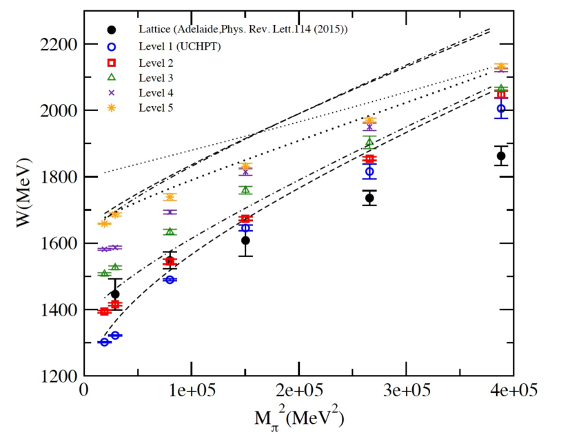
Results are shown in Fig. 1 for the first five energy levels predicted from U$\chi$PT (solid lines). The lattice data of hall are shown as black dots. They correspond to a size of the box of around $L\simeq 3$ fm (see Table 2). For the physical point in this figure we also take $L=3$ fm. There is good agreement between the U$\chi$PT prediction of the second energy level and the lattice data for masses below $400$ MeV. For larger masses there are discrepancies which are discussed later on this section. However, for the two lowest lattice pion masses, U$\chi$PT predicts an additional level below the $\pi\Sigma$ threshold, associated with an attractive $\pi\Sigma$ scattering length. The level is not only present in common U$\chi$PT calculations that all predict an attractive $\pi\Sigma$ scattering length, it is also found in the finite-volume version of the dynamical coupled-channel model of Ref. Doring:2011ip . In Ref. Doring:2011ip , that represents the first finite-volume implementation of dynamical coupled-channel models, the attractive $\pi\Sigma$ interaction arises from explicit $t$- and $u$- channel diagrams. This lowest level is absent in the lattice simulation of Ref. hall as Fig. 1 shows. If that finding is confirmed, it represents a serious challenge for all discussed hadronic models. However, as the lowest state is a scattering state, maybe it has simply not been detected in Ref. hall , which relies on quark operators to extract the finite-volume spectrum. Level extraction using meson-baryon operators instead of quark operators could help detecting this scattering state. Meson-baryon channels that have large overlap with the various eigenstates are identified later in this section.

In the chiral extrapolation we include the quark mass dependences of the decay constants $f_{\pi},f_{K},f_{\eta}$ but cannot specify the quark mass dependence of the subtraction constants $\alpha_{i}$. To estimate the uncertainties from this source we vary each subtraction constant $\alpha$ gradually for increasing pion masses by $5\%$, $10\%$, $15\%$, $20\%$ and $25\%$ corresponding to sets 1 to 5 in Table 2 respectively. Also, to account for uncertainties in the chiral extrapolation of the decay constants $f_{\pi}$, $f_{K}$ and $f_{\eta}$, we vary them by $5\%$, for all sets (since we considered here pion mass dependence). Fig. 1 shows that even with these rather large changes the predicted levels are still less uncertain that the values from the lattice simulation. However, the discrepancy for pion masses larger than $400$ MeV persists. We could attribute this to different sources like the missing NLO in our model, or to the fact that the chiral extrapolation breaks down at high pion masses due to a genuine component, or that the discrepancies come from other sources intrinsic to the lattice computation like underestimated errors.

IV.2 Channel dynamics of levels and poles

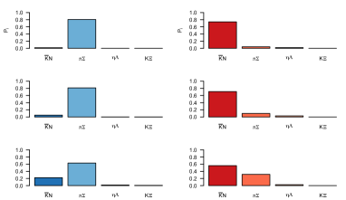
In order to understand the role of the meson-baryon channels in the extracted energy levels, we evaluate the couplings $\tilde{g}_{i}$, and the magnitudes $\tilde{P}_{i}=-\left(\tilde{g}_{i}^{2}\frac{\partial\tilde{G}_{i}}{\partial W}\right)_{W=W_{0}}$, $1-\tilde{Z}$, and $\tilde{Z}$, of Eq. (14) at the pole position. These quantities are shown in Table 3 for the physical mass ($L=3$ fm) and sets 1 to 3 of quark masses shown in Table 2 (at higher masses the chiral prediction becomes very uncertain and no values are quoted). The part which is related to the energy dependence of the potential is generally small, $\tilde{Z}\simeq 0-0.3$, and the weights of the channels $\tilde{P}_{i}$’s are between $0$ and $1$, like in the infinite volume for bound states. The $\tilde{P}_{i}$’s are diagrammatically represented in Fig. 2. Here, the left column of bar diagrams in blue represents the weights $\tilde{P}_{i}$ of the lowest energy level, while the following columns represent the levels $2$ to $5$ with the same color coding as in Fig. 1. Every level is depicted for pion masses in the range $170-388$ MeV from top to bottom corresponding to sets $1$ to $3$ in Table 2. The $\pi\Sigma$ channel dominates the lowest level. The relative weights $\tilde{P}_{l}$ for the $\eta\Lambda$ and $K\Xi$ are almost zero for the lowest state and for low pion masses (set 1). This confirms the discussed property of the $\tilde{P}_{l}$ suppressing effectively the irrelevant channels that open at much higher energies (compare with the corresponding values for the $\tilde{g}_{i}$ in Table 3). Also, it is quite natural that the lowest state has a dominant $\pi\Sigma$ content, as it is a threshold level below the $\pi\Sigma$ threshold associated with an attractive $\pi\Sigma$ interaction. For larger quark masses, this trend is inverted and the $\bar{K}N$ strength becomes larger. On the other hand, the second energy level (second column in Fig. 2) shows a significant dominance of the $\bar{K}N$ component, with $\tilde{g}_{\bar{K}N}$ and $\tilde{P}_{\bar{K}N}$ both larger, if the pion mass is not very high. Although we cannot identify finite-volume energy eigenstates with resonances, the $\bar{K}N$ dominance of the second eigenstate is in line with the second $\Lambda(1405)$ pole being predominantly generated from the $\bar{K}N$ channel (cf. Table 1).

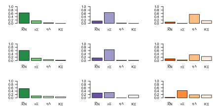
From Fig. 1, is clear that the first two lattice data points in Fig. 1 correspond to the second energy level, for which the $\bar{K}N$ component clearly dominates, while the third lattice data point could belong to either the first or second energy level predicted from U$\chi$PT. For the third energy level, both $\tilde{g}_{i}$ and $\tilde{P}_{i}$ are larger for the $\bar{K}N$ component, while the $\pi\Sigma$ channel dominates the fourth energy level.

In the fifth energy level, these two channels become irrelevant, and the coupling strengths to $\eta\Lambda$ and $K\Xi$ dominate. At the physical point, this level is very close to the real part of the pole position of the $\Lambda(1670)$ (cf. Table 1). In the infinite volume, that resonance appears as a quasibound $K\Xi$ state with relatively small $\bar{K}N$ and $\pi\Sigma$ branching ratios as Table 1 shows. The overlap with the $\eta\Lambda$ channel is not small although the branching ratio to this channel is only moderate due to reduced phase space. In the finite volume, the situation is different because the weight of the $K\Xi$ channel in the wave function, $\tilde{P}_{l}$, is reduced as Table 3 shows. At higher pion masses, the fifth eigenstate stays close to the non-interacting $\eta\Lambda$ threshold (Fig. 1), while the pole of the $\Lambda(1670)$ moves considerably away from the $\eta\Lambda$ threshold (Fig. 3). It is thus, not possible to associate the fifth finite-volume eigenstate with the infinite-volume $\Lambda(1670)$ resonance.

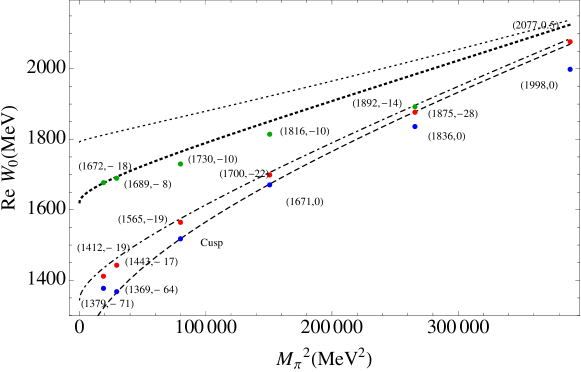
We can compare these results with the calculation in the infinite volume using the formalism described in Section II together with the SU(3) chiral extrapolation explained before. The results are shown in Fig. 3. Here, the pole positions in the infinite volume as a function of the pion mass are depicted. The four lines represent the $\pi\Sigma$, $\bar{K}N$, $\eta\Lambda$ and $K\Xi$ thresholds. For masses close to the physical point, the lowest state is a resonance above the $\pi\Sigma$ threshold. When the mass of the pion increases, the lower state becomes a cusp, i.e., the pole is close to threshold, but on a sheet that is not directly accessible from the physical axis. When the pion mass increases further, it becomes a bound state. The second pole of the $\Lambda(1405)$ is always below and close to the $\bar{K}N$ threshold for all pion masses considered. A third state appears at higher energies. This state couples more to the channels $\eta\Lambda$ and $K\Xi$, with larger coupling strength to $K\Xi$. This state is identified with the $\Lambda(1670)$ bennhold ; Doring:2011ip . In Table 4, we show the comparison between the two lowest pole positions and coupling constants in the infinite and finite volume. For the physical pion mass, we have taken here larger boxes, $L=4$ fm. In this table, $b_{\bar{K}N}$ and $b_{\pi\Sigma}$ denote the distances to the $\bar{K}N$ and $\pi\Sigma$ thresholds, where the negative sign means that the state is above threshold. For masses below $400$ MeV, we observe that the second state in the finite volume has a dominant $\bar{K}N$ component, and is between the $\pi\Sigma$ and $\bar{K}N$ thresholds. It shares these properties with the higher-lying pole of the $\Lambda(1405)$ in the infinite volume. We can understand the proximity of finite- and infinite-volume states as follows: the second $\Lambda(1405)$ pole is a quasi- bound $\bar{K}N$ state with little influence from the $\pi\Sigma$ channel. In the finite volume, the eigenstate appears therefore almost as a bound state. In the limit of zero $\pi\Sigma$ coupling, the position of finite- and infinite-volume poles would differ only by exponentially suppressed corrections scaling with the binding momentum. On the contrary, the lower state shows very different properties in the infinite volume limit and in the box. As discussed, for low pion masses, the finite-volume state below the $\pi\Sigma$ threshold is related to the lower $\Lambda(1405)$ pole only insofar, that it indicates the attractive $\pi\Sigma$ interaction leading to the generation of the pole in the infinite volume (at a very different position). For high pion masses, the lower $\Lambda(1405)$ pole in the infinite volume limit becomes a bound state, and then the couplings to all the channels become very similar to the ones in the box as one can see from Table 4. However, in this case the masses of the poles are very far away from the lattice data of Ref. hall which can be due to different reasons as discussed before.

Figure 1: Comparison between the U$\chi$PT prediction for the first five energy levels (solid lines) and the lattice data of Ref. hall , for the physical set ($L=3$ fm) and sets 1 to 5, as shown in Table 2. The errors of our results are obtained by varying subtraction constants and meson decay constants as described in Sec. IV. Here, the dashed, dot-dashed lines represent $\pi\Sigma$ and $\bar{K}N$ non-interacting levels respectively (the first two levels are depicted), while the thick-dotted and dotted lines, show the first $\eta\Lambda$ and $K\Xi$ non-interacting levels, respectively.

Set	$L(fm)$	$m_{\pi}$	$m_{K}$	$m_{\eta}$	$M_{N}$	$M_{\Lambda}$	$M_{\Sigma}$	$M_{\Xi}$	$f_{\pi}$	$f_{K}$	$f_{\eta}$
1	2.99	170.29	495.78	563.97	962.2	1135.8	1181.5	1323.6	94.5	113.2	122.1
2	3.04	282.84	523.26	581.72	1058.7	1173.4	1235.5	1332.8	102.5	116.1	122.3
3	3.08	387.81	559.46	605.97	1150.1	1261.0	1292.4	1377.4	109.5	118.5	122.6
4	3.23	515.56	609.75	638.07	1274.5	1333.4	1353.5	1401.8	116.3	120.6	122.4
5	3.27	623.14	670.08	685.01	1420.3	1434.2	1449.8	1472.4	120.1	121.9	122.6

Table 2: Pseudoscalar meson decay constants obtained from SU(3) chiral extrapolation with the masses from hall . Units are MeV.

	$\bar{K}N$	$\pi\Sigma$	$\eta\Lambda$	$K\Xi$	$1-\tilde{Z}$	$\tilde{Z}$
$W_{0}=1302(1)$
$\tilde{g}_{i}$	$-0.69(5)$	$0.80(3)$	$-0.15(2)$	$0.080(2)$
$\tilde{P}_{l}$	$0.020(3)$	$0.77(1)$	$0.0004(1)$	$0.000090(5)$	$0.79(1)$	$0.21(1)$
$W_{0}=1394(4)$
$\tilde{g}_{i}$	$1.9(1)$	$-0.388(5)$	$0.94(5)$	$-0.061(6)$
$\tilde{P}_{l}$	$0.76(2)$	$0.046(6)$	$0.021(2)$	$0.00007(1)$	$0.83(2)$	$0.17(2)$
$W_{0}=1507(4)$
$\tilde{g}_{i}$	$2.34(2)$	$-0.92(7)$	$1.10(3)$	$-0.39(2)$
$\tilde{P}_{l}$	$0.68(2)$	$0.10(1)$	$0.046(3)$	$0.0036(5)$	$0.83(1)$	$0.17(1)$
$W_{0}=1582(3)$
$\tilde{g}_{i}$	$0.64(5)$	$1.93(3)$	$0.43(4)$	$0.45(4)$
$\tilde{P}_{l}$	$0.09(1)$	$0.73(1)$	$0.014(2)$	$0.006(1)$	$0.840(3)$	$0.160(3)$
$W_{0}=1659(2)$
$\tilde{g}_{i}$	$0.09(1)$	$-0.04(1)$	$-0.3(1)$	$1.3(1)$
$\tilde{P}_{l}$	$0.069(6)$	$0.002(1)$	$0.76(5)$	$0.077(17)$	$0.91(4)$	$0.09(4)$
$W_{0}=1322(2)$
$\tilde{g}_{i}$	$-0.65(5)$	$0.90(4)$	$-0.14(2)$	$0.105(3)$
$\tilde{P}_{l}$	$0.017(3)$	$0.80(1)$	$0.0003(1)$	$0.00017(1)$	$0.82(1)$	$0.18(1)$
$W_{0}=1416(4)$
$\tilde{g}_{i}$	$1.94(13)$	$-0.43(1)$	$0.96(5)$	$-0.07(2)$
$\tilde{P}_{l}$	$0.76(3)$	$0.047(2)$	$0.021(2)$	$0.0001(5)$	$0.83(3)$	$0.17(3)$
$W_{0}=1526(5)$
$\tilde{g}_{i}$	$2.20(5)$	$-1.14(15)$	$1.02(4)$	$-0.5(1)$
$\tilde{P}_{l}$	$0.64(5)$	$0.16(5)$	$0.037(3)$	$0.004(1)$	$0.841(6)$	$0.159(6)$
$W_{0}=1587(4)$
$\tilde{g}_{i}$	$0.94(11)$	$1.83(7)$	$0.59(7)$	$0.41(6)$
$\tilde{P}_{l}$	$0.15(3)$	$0.66(4)$	$0.019(5)$	$0.005(1)$	$0.834(7)$	$0.166(7)$
$W_{0}=1686(5)$
$\tilde{g}_{i}$	$0.07(4)$	$-0.034(18)$	$-0.59(16)$	$1.8(2)$
$\tilde{P}_{l}$	$0.079(8)$	$0.009(5)$	$0.56(11)$	$0.16(4)$	$0.81(6)$	$0.19(6)$

	$\bar{K}N$	$\pi\Sigma$	$\eta\Lambda$	$K\Xi$	$1-\tilde{Z}$	$\tilde{Z}$
$W_{0}=1490(3)$
$\tilde{g}_{i}$	$-0.85(19)$	$1.14(9)$	$-0.3(1)$	$0.29(3)$
$\tilde{P}_{l}$	$0.05(2)$	$0.83(4)$	$0.003(2)$	$0.0017(3)$	$0.88(2)$	$0.12(2)$
$W_{0}=1544(7)$
$\tilde{g}_{i}$	$1.78(18)$	$-0.31(4)$	$1.0(1)$	$-0.14(6)$
$\tilde{P}_{l}$	$0.74(8)$	$0.09(4)$	$0.03(5)$	$0.0006(4)$	$0.86(3)$	$0.14(3)$
$W_{0}=1633(8)$
$\tilde{g}_{i}$	$1.85(15)$	$-1.0(2)$	$1.13(11)$	$-0.94(3)$
$\tilde{P}_{l}$	$0.60(1)$	$0.14(6)$	$0.06(1)$	$0.03(2)$	$0.83(4)$	$0.17(4)$
$W_{0}=1693(6)$
$\tilde{g}_{i}$	$1.00(18)$	$1.72(12)$	$0.43(14)$	$0.66(21)$
$\tilde{P}_{l}$	$0.18(6)$	$0.63(8)$	$0.02(1)$	$0.02(1)$	$0.85(2)$	$0.15(2)$
$W_{0}=1739(9)$
$\tilde{g}_{i}$	$0.51(12)$	$-0.3(2)$	$-0.6(2)$	$1.9(3)$
$\tilde{P}_{l}$	$0.10(2)$	$0.05(5)$	$0.43(18)$	$0.20(5)$	$0.78(8)$	$0.22(8)$
$W_{0}=1646(8)$
$\tilde{g}_{i}$	$-1.47(5)$	$1.26(12)$	$-0.8(3)$	$0.51(15)$
$\tilde{P}_{l}$	$0.23(12)$	$0.59(20)$	$0.02(2)$	$0.007(5)$	$0.85(7)$	$0.15(7)$
$W_{0}=1674(5)$
$\tilde{g}_{i}$	$1.24(23)$	$0.28(23)$	$0.76(15)$	$-1.1(1)$
$\tilde{P}_{l}$	$0.56(22)$	$0.34(22)$	$0.021(7)$	$0.0004(5)$	$0.92(4)$	$0.08(4)$
$W_{0}=1759(11)$
$\tilde{g}_{i}$	$1.74(27)$	$-0.86(27)$	$1.17(34)$	$-1.1(7)$
$\tilde{P}_{l}$	$0.56(11)$	$0.12(5)$	$0.08(3)$	$0.06(4)$	$0.82(5)$	$0.18(5)$
$W_{0}=1815(11)$
$\tilde{g}_{i}$	$1.2(3)$	$1.0(4)$	$-0.29(16)$	$1.9(3)$
$\tilde{P}_{l}$	$0.24(1)$	$0.33(16)$	$0.01(1)$	$0.18(5)$	$0.76(9)$	$0.24(9)$
$W_{0}=1836(8)$
$\tilde{g}_{i}$	$0.42(13)$	$-0.8(4)$	$-0.65(16)$	$1.8(3)$
$\tilde{P}_{l}$	$0.06(4)$	$0.4(2)$	$0.17(11)$	$0.19(8)$	$0.82(4)$	$0.18(4)$

Table 3: Pole positions, $W_{0}$, couplings, $\tilde{g}_{i}$, $\tilde{P}_{l}$’s, $1-\tilde{Z}$ and $\tilde{Z}$ in Eq. (14), for the five energy levels predicted from U$\chi$PT in Fig. 1. From left-top to bottom, it refers to the physical set and set 1, and from right-top to bottom, sets 2 and 3 in Table 2. Pole positions are given in units of MeV. The errors are obtained by varying subtraction and meson decay constants as described in Sec. IV.1.

Figure 2: Weights of the different channels, $\tilde{P}_{i}$’s (first term on the right hand side of Eq. (14) for the first five energy levels (from left to right) and pion masses from $170$ to $388$ MeV (sets 1 to 3 in Table 2, from top to bottom).

Figure 3: Behavior of the real part of the pole positions, $\mathrm{Re}\,W_{0}$, found in the $T$-matrix in the infinite volume with the $M^{2}_{\pi}$, for the physical, and 1 to 5 sets. The numbers in parenthesis indicate the pole positions including the imaginary parts. The lines show the $\pi\Sigma$, $\bar{K}N$, $\eta\Lambda$ and $K\Xi$ thresholds.

Infinite volume Set Channel Pole $|g_{i}|$ $b_{\bar{K}N}$ $b_{\pi\Sigma}$ (MeV) $\bar{K}N$ $\pi\Sigma$ $\eta\Lambda$ $K\Xi$ (MeV) (MeV) Phy. 1379-i 71 2.20 3.1 0.8 0.5 56 -48 1412-i 19 3.1 1.7 1.5 0.3 23 -81 1 1369-i 64 1.9 2.9 0.6 0.5 89 -17 1443-i 17 2.6 1.35 1.32 0.3 15 -91 2 Cusp at 1518.34 64 0 1565-i 19 2.5 1.5 1.4 0.5 17 -47 3 1671 2.0 1.3 1.1 0.6 39 9 1700-i 22 2.0 1.6 1.3 0.7 10 -20 4 1836 1.9 1.2 1.7 1.8 48 33 1875-i 28 1.3 1.8 1.6 1.7 9 -6 5 1998 0.9 0.8 1.9 2.9 92 75 2077-i 0.5 2.1 0.4 0.3 1.1 13 -4

Finite volume

	Channel
Pole	$|\tilde{g}_{i}|$				$b_{\bar{K}N}$	$b_{\pi\Sigma}$
(MeV)	$\bar{K}N$	$\pi\Sigma$	$\eta\Lambda$	$K\Xi$	(MeV)	(MeV)
1322	0.5	0.6	0.1	0.07	113	9
1401	2.2	1.0	1.0	0.2	34	-70
1322	0.6	0.9	0.1	0.1	136	30
1417	1.9	0.4	0.9	0.06	41	-65
1489	0.9	1.2	0.3	0.3	93	29
1541	1.9	0.3	1.0	0.2	41	-23
1649	1.4	1.3	0.7	0.5	61	31
1676	1.5	0.1	0.9	0.06	34	4
1829	1.8	1.2	1.5	1.5	55	40
1859	0.9	0.5	0.6	0.09	25	10
1997	1.0	0.9	1.9	2.9	93	76
2062	0.9	0.7	0.2	0.9	28	11

Table 4: Pole positions and couplings of the states $|g_{i}|$ in the infinite (left, A) and finite (right, B) volume for all sets. Note that for the physical set in the finite volume (“Phy.”) we have taken larger volumes ($L=4$ fm) for the values that are shown in this table. For the other sets of pion masses of Ref. hall , $L\simeq 3$ fm is used. It should be stressed that finite- and infinite-volume poles cannot be directly identified with each other.

Figure 4: Real (solid lines) and imaginary parts (dashed lines) of the meson-baryon scattering amplitude of the four coupled channels $\bar{K}N$, $\pi\Sigma$, $\eta\Lambda$ and $K\Xi$. From top to bottom, the figures correspond to physical pion mass and sets 1 to 3 of Table 2. The left column corresponds to the $T_{\bar{K}N\to\bar{K}N}$ amplitude, the central column corresponds to the transition $T_{\bar{K}N\to\pi\Sigma}$ and the right column to $T_{\pi\Sigma\to\pi\Sigma}$.

Meson-baryon scattering amplitudes for different pion masses in the infinite volume limit

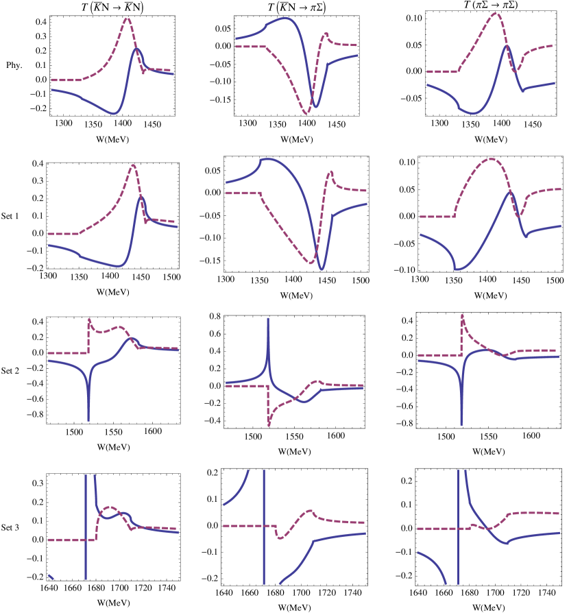
Finally, we provide the infinite-volume scattering amplitudes for strangeness=$-1$ in Fig. 4. Every row shows the real (solid lines) and imaginary part (dashed lines) of the scattering amplitude, $T_{\bar{K}N\to\bar{K}N},T_{\bar{K}N\to\pi\Sigma}$ and $T_{\pi\Sigma\to\pi\Sigma}$. The first row shows the amplitude for the physical pion mass, while the second to fourth rows correspond to pion masses of $170$, $282$ and $388$ MeV (first three sets in Table 2). For the physical set, these amplitudes are very similar to the ones obtained in the work of Ref. bennhold , where we observe the presence of two resonances related to the two poles near the energy of the $\Lambda(1405)$. For higher pion masses the lighter pole of the $\Lambda(1405)$ first becomes a cusp (third row) and then a bound state (fourth row). The heavier pole of the $\Lambda(1405)$ couples predominantly to the $\bar{K}N$ channel as the figure in the upper left corner shows. As the pion mass increases, the pole remains close to the $\bar{K}N$ threshold as a quasi-bound state.

The fact that the second pole of the $\Lambda(1405)$ always appears close to the $\bar{K}N$ threshold may be due to that the kaon mass, which controls the strength of the $\bar{K}N\to\bar{K}N$ Weinberg-Tomozawa term, does not change much, so that the properties of the bound state also do not experience much variations. In contrast, the $\pi\Sigma\to\pi\Sigma$ Weinberg-Tomozawa interaction becomes significantly stronger with increasing pion mass, changing drastically the nature of the lower state from resonance to bound state.

V Conclusions

The quark mass dependence of the energy levels in a box for the coupled channels with $J^{P}=\frac{1}{2}^{-},I=0,S=-1$ has been studied, using the Weinberg-Tomozawa term from the lowest order $\chi$PT interaction. This dependence has been compared to the lattice data of Ref. hall and extrapolated to the infinite volume. U$\chi$PT predicts a two-pole structure for the $\Lambda(1405)$. In the finite volume, two energy levels close to the $\pi\Sigma$ and $\bar{K}N$ thresholds are found. The second energy level agrees well with the lattice data of Ref. hall for pion masses below $400$ MeV, in the estimated limit of applicability of the present approach. This energy level shows a large coupling and overlap with the $\bar{K}N$ channel and has similar properties as the higher pole of the $\Lambda(1405)$. The state remains quasi-bound in the $\bar{K}N$ channel and close to its threshold, as the pion mass increases. Thus, the lattice data of Ref. hall are not in contradiction with the two-pole hypothesis for the $\Lambda(1405)$. Yet, these data proof by no means that hypothesis. For this, a few remaining obstacles need to be addressed: The first problem is the absence of the $\pi\Sigma$ threshold level in the lattice calculation of Ref. hall , that appears here below the $\pi\Sigma$ threshold, indicating an attractive $\pi\Sigma$ interaction. In the infinite volume, this attraction leads to the generation of a second (lighter) pole of the $\Lambda(1405)$. This behavior is universal in U$\chi$PT calculations, and also present in some dynamical coupled-channel approaches. Here, we have assumed that this absence is due to the absence of meson-baryon operators in the operator base used in Ref.  hall . To propose suitable meson-baryon operators for the detection of the threshold level, we have considered the finite-volume analog of $\tilde{P}_{l}$ that specify the relative weight of a channel in a state’s wave function. It turns out that an operator of the $\pi\Sigma$ type is most suited to detect the level in future lattice simulations. Indeed, the precise location of that level would specify the size of attraction in the $\pi\Sigma$ channel at threshold and help to pin down the location of the lighter $\Lambda(1405)$ pole that is notoriously difficult to determine. Also, a precise determination of the pole positions from lattice data requires to populate the region between the $\pi\Sigma$ and $\bar{K}N$ thresholds with more lattice eigenvalues, using, e.g., moving frames and asymmetric boxes MartinezTorres:2012yi . Also, higher-order U$\chi$PT calculations along the lines of Refs. Guo:2012vv ; Ikeda:2012au ; Mai:2012dt will be needed to assess theoretical uncertainties in direct fits to future lattice data.

Appendix
SU(3) chiral extrapolation

Chiral symmetry is explicitly broken and gives rise to masses of the quarks $u,d,s$ different from zero. Then, the Goldstone bosons acquire masses which at leading order are related to the chiral condensate and are denoted here as $M_{0\pi}$, $M_{0K}$ and $M_{0\eta}$. To one loop, the masses of the Goldstone bosons carry corrections and the physical masses can be expressed as a function of the leading order masses ($M_{0}$), LEC’s ($L^{r}$) and pseudoscalar decay constants ($f$). The following formulas for the pseudoscalar masses, derived from the SU(3) chiral extrapolation are taking from Ref. jenifer , which is based on chiral perturbation theory Gasser:1984gg ,

$$M_{\pi}^{2}=M_{0\,\pi}^{2}\left[1+\mu_{\pi}-\frac{\mu_{\eta}}{3}+\frac{16M_{0\,K}^{2}}{f_{0}^{2}}\left(2L_{6}^{r}-L_{4}^{r}\right)\right.$$

$$+\left.\frac{8M_{0\,\pi}^{2}}{f_{0}^{2}}\left(2L_{6}^{r}+2L_{8}^{r}-L_{4}^{r}-L_{5}^{r}\right)\right],$$ (15)

$$M^{2}_{K}=M^{2}_{0\,K}\left[1+\frac{2\mu_{\eta}}{3}+\frac{8M_{0\,\pi}^{2}}{f_{0}^{2}}\left(2L_{6}^{r}-L_{4}^{r}\right)\right.$$

$$+\left.\frac{8M_{0\,K}^{2}}{f_{0}^{2}}\left(4L_{6}^{r}+2L_{8}^{r}-2L_{4}^{r}-L_{5}^{r}\right)\right],$$ (16)

$$M^{2}_{\eta}=M^{2}_{0\,\eta}\left[1+2\mu_{K}-\frac{4}{3}\mu_{\eta}+\frac{8M^{2}_{0\,\eta}}{f_{0}^{2}}(2L_{8}^{r}-L_{5}^{r})\right.$$

$$+\left.\frac{8}{f_{0}^{2}}(2M^{2}_{0\,K}+M^{2}_{0\,\pi})(2L_{6}^{r}-L_{4}^{r})\right]$$

$$+M^{2}_{0\,\pi}\left[-\mu_{\pi}+\frac{2}{3}\mu_{K}+\frac{1}{3}\mu_{\eta}\right]$$

$$+\frac{128}{9f_{0}^{2}}(M^{2}_{0\,K}-M^{2}_{0\,\pi})^{2}(3L_{7}+L_{8}^{r}),$$ (17)

with

$$\hskip 14.22636pt\mu_{P}=\frac{M_{0\,P}^{2}}{32\pi^{2}f_{0}^{2}}\log\frac{M_{0\,P}^{2}}{\mu^{2}},\qquad P=\pi,K,\eta\ .$$ (18)

In the above equations $f_{0}$ is the pion decay constant in the chiral limit, $4\pi f_{0}\simeq 1.2$ GeV, $\mu$ is the regularization scale, commonly fixed at $\mu=M_{\rho}$, and $L^{r}_{i}$’s, with $i=1,8$, are the Low Energy Constants which multiply the tree level diagrams of $\mathcal{O}(p^{4})$ present in the next to leading order $t_{4}(s)$ term in the $\chi PT$ expansion of the amplitude for meson-meson scattering ($t(s)=t_{2}(s)+t_{4}(s)+...$, $t_{2k}=\mathcal{O}(p^{2k})$).

On the other hand, the decay constants evaluated to one loop SU(3) $\chi PT$, are expressed in terms of the masses at leading order as

$$f_{\pi}=f_{0}\left[1-2\mu_{\pi}-\mu_{K}+\frac{4M_{0\,\pi}^{2}}{f_{0}^{2}}\left(L_{4}^{r}+L_{5}^{r}\right)+\frac{8M_{0\,K}^{2}}{f_{0}^{2}}L_{4}^{r}\right],$$

(19)

$$f_{K}=f_{0}\left[1-\frac{3\mu_{\pi}}{4}-\frac{3\mu_{K}}{2}-\frac{3\mu_{\eta}}{4}+\frac{4M_{0\,\pi}^{2}}{f_{0}^{2}}L_{4}^{r}\right.$$

$$+\left.\frac{4M_{0\,K}^{2}}{f_{0}^{2}}\left(2L_{4}^{r}+L_{5}^{r}\right)\right],$$ (20)

$$f_{\eta}=f_{0}\left[1-3\mu_{K}+\frac{4L_{4}^{r}}{f_{0}^{2}}\left(M_{0\,\pi}^{2}+2M_{0\,K}^{2}\right)+\frac{4M_{0\,\eta}^{2}}{f_{0}^{2}}L_{5}^{r}\right]\ .$$

(21)

The $L^{r}_{i}$’s values used here are taken from Fit I of Ref. jenifer to experiment and lattice data (shown in Table 1 of Ref. jenifer ).

In order to evaluate the meson decay constants for the different sets of Table 2, first Eqs. (15), (16), (19) and (20) are evaluated at the physical point (Table 2), obtaining the values of the four variables, $M_{0\pi}$, $M_{0K}$ $M_{0\eta}$ and $f_{0}$. In these sets of equations, the LEC $L^{r}_{7}$ does not appear. Once these constants are known, $L^{r}_{7}$ is fixed to obtain the mass of the $\eta$ at the physical point, given by Eq. (17). This gives as a result, $L^{r}_{7}=-0.423\times 10^{-3}$, very close to the one obtained in jenifer ($-0.43\times 10^{-3}$). For $f_{0}$, a value of $79.2$ is obtained, and using the formulas of Eqs. (15)-(21), we evaluate the $M_{0}$’s and $f$’s for $\pi$, $K$ and $\eta$ for every set of masses in Table 2. The decay constants obtained are shown in Table 2 of the Results Section.

References

- (1) N. Isgur and G. Karl, Phys. Rev. D 18, 4187 (1978).
- (2) T. Inoue, Nucl. Phys. A 790, 530 (2007).
- (3) R. H. Dalitz and S. F. Tuan, Annals Phys. 10, 307 (1960).
- (4) R. H. Dalitz, T. C. Wong and G. Rajasekaran, Phys. Rev. 153, 1617 (1967).
- (5) E. A. Veit, B. K. Jennings, A. W. Thomas and R. C. Barrett, Phys. Rev. D 31, 1033 (1985).
- (6) P. B. Siegel and B. Saghai, Phys. Rev. C 52, 392 (1995).
- (7) K. Tanaka and A. Suzuki, Phys. Rev. C 45, 2068 (1992).
- (8) Y. A. Chao, R. W. Kraemer, D. W. Thomas and B. R. Martin, Nucl. Phys. B 56, 46 (1973).
- (9) R. H. Dalitz and J. G. McGinley, Proceedings of the international Conference on Hypernuclear and Kaon Physics (North Holland, Heidelberg, 1982)
- (10) H. Kamano, S. X. Nakamura, T.-S. H. Lee and T. Sato, Phys. Rev. C 90, 065204 (2014).
- (11) H. Kamano, S. X. Nakamura, T.-S. H. Lee and T. Sato, Phys. Rev. C 92, no. 2, 025205 (2015).
- (12) H. Zhang, J. Tulpan, M. Shrestha and D. M. Manley, Phys. Rev. C 88, 035204 (2013).
- (13) C. Fernández-Ramírez, I. V. Danilkin, D. M. Manley, V. Mathieu and A. P. Szczepaniak, Phys. Rev. D 93, no. 3, 034029 (2016).
- (14) B. C. Jackson, Y. Oh, H. Haberzettl and K. Nakayama, Phys. Rev. C 91, 065208 (2015).
- (15) A. Feijoo, V. K. Magas and A. Ramos, Phys. Rev. C 92, 015206 (2015).
- (16) W. J. Briscoe, M. Döring, H. Haberzettl, D. M. Manley, M. Naruki, I. I. Strakovsky and E. S. Swanson, Eur. Phys. J. A 51, 129 (2015).
- (17) J. Gasser, V. E. Lyubovitskij and A. Rusetsky, Phys. Rept. 456, 167 (2008).
- (18) B. K. Jennings, Phys. Lett. B 176, 229 (1986).
- (19) M. Arima and K. Yazaki, Nucl. Phys. A 506, 553 (1990).
- (20) M. Arima, S. Matsui and K. Shimizu, Phys. Rev. C 49, 2831 (1994).
- (21) G. l. He and R. H. Landau, Phys. Rev. C 48, 3047 (1993).
- (22) K. S. Kumar and Y. Nogami, Phys. Rev. D 21, 1834 (1980).
- (23) J. Schnick and R. H. Landau, Phys. Rev. Lett. 58, 1719 (1987).
- (24) P. J. Fink, Jr., G. He, R. H. Landau and J. W. Schnick, Phys. Rev. C 41, 2720 (1990).
- (25) M. Iwasaki, R. S. Hayano, T. M. Ito, S. N. Nakamura, T. P. Terada, D. R. Gill, L. Lee and A. Olin et al., Phys. Rev. Lett. 78, 3067 (1997).
- (26) T. M. Ito, R. S. Hayano, S. N. Nakamura, T. P. Terada, M. Iwasaki, D. R. Gill, L. Lee and A. Olin et al., Phys. Rev. C 58, 2366 (1998).
- (27) S. Deser, M. L. Goldberger, K. Baumann and W. E. Thirring, Phys. Rev. 96, 774 (1954).
- (28) U.-G. Meißner, U. Raha and A. Rusetsky, Eur. Phys. J. C 35, 349 (2004).
- (29) M. Bazzi, G. Beer, L. Bombelli, A. M. Bragadireanu, M. Cargnelli, G. Corradi, C. Curceanu (Petrascu) and A. d’Uffizi et al., Phys. Lett. B 704, 113 (2011).
- (30) G. Beer et al. [DEAR Collaboration], Phys. Rev. Lett. 94, 212302 (2005).
- (31) Y. Ikeda, T. Hyodo and W. Weise, Nucl. Phys. A 881, 98 (2012).
- (32) B. Borasoy, R. Nißler and W. Weise, Eur. Phys. J. A 25, 79 (2005).
- (33) J. A. Oller, J. Prades and M. Verbeni, Phys. Rev. Lett. 95, 172502 (2005).
- (34) J. A. Oller, Eur. Phys. J. A 28, 63 (2006)
- (35) M. Mai and U. G. Meißner, Nucl. Phys. A 900, 51 (2013).
- (36) Z. H. Guo and J. A. Oller, Phys. Rev. C 87, 035202 (2013).
- (37) Y. Kamiya, K. Miyahara, S. Ohnishi, Y. Ikeda, T. Hyodo, E. Oset and W. Weise, arXiv:1602.08852 [hep-ph].
- (38) A. Cieplý, M. Mai, U.-G. Meißner and J. Smejkal, arXiv:1603.02531 [hep-ph].
- (39) J. A. Oller and U.-G. Meißner, Phys. Lett. B 500, 263 (2001).
- (40) M. Döring and U.-G. Meißner, Phys. Lett. B 704, 663 (2011).
- (41) M. Mai, V. Baru, E. Epelbaum and A. Rusetsky, Phys. Rev. D 91, 054016 (2015).
- (42) N. Kaiser, T. Waas and W. Weise, Nucl. Phys. A 612, 297 (1997).
- (43) E. Oset, A. Ramos and C. Bennhold, Phys. Lett. B 527, 99 (2002).
- (44) N. Kaiser, P. B. Siegel and W. Weise, Nucl. Phys. A594, 325 (1995).
- (45) E. Oset and A. Ramos, Nucl. Phys. A 635, 99 (1998).
- (46) D. Jido, A. Hosaka, J. C. Nacher, E. Oset and A. Ramos, Phys. Rev. C 66, 025203 (2002).
- (47) D. Jido, J. A. Oller, E. Oset, A. Ramos and U.-G. Meißner, Nucl. Phys. A 725, 181 (2003).
- (48) C. Garcia-Recio, J. Nieves, E. Ruiz Arriola and M. J. Vicente Vacas, Phys. Rev. D 67, 076009 (2003).
- (49) M. Döring, D. Jido and E. Oset, Eur. Phys. J. A 45, 319 (2010).
- (50) B. Borasoy, U.-G. Meißner and R. Nißler, Phys. Rev. C 74, 055201 (2006).
- (51) L. S. Geng and E. Oset, Eur. Phys. J. A 34, 405 (2007).
- (52) V. K. Magas, E. Oset and A. Ramos, Phys. Rev. Lett. 95, 052301 (2005).
- (53) S. Prakhov et al. [Crystall Ball Collaboration], Phys. Rev. C 70, 034605 (2004).
- (54) L. S. Geng, E. Oset and M. Döring, Eur. Phys. J. A 32, 201 (2007).
- (55) T. Hyodo, A. Hosaka, E. Oset, A. Ramos and M. J. Vicente Vacas, Phys. Rev. C 68, 065203 (2003).
- (56) T. Hyodo, A. Hosaka, M. J. Vicente Vacas and E. Oset, Phys. Lett. B 593, 75 (2004).
- (57) D. Jido, E. Oset and T. Sekihara, Eur. Phys. J. A 42, 257 (2009).
- (58) T. Sekihara, T. Hyodo and D. Jido, PTEP 2015, 063D04 (2015).
- (59) T. Hyodo, D. Jido and A. Hosaka, Phys. Rev. C 78, 025203 (2008).
- (60) C. Fernández-Ramírez, I. V. Danilkin, V. Mathieu and A. P. Szczepaniak, Phys. Rev. D 93, 074015 (2016).
- (61) K. Moriya et al. [CLAS Collaboration], Phys. Rev. C 87, 035206 (2013).
- (62) K. Moriya et al. [CLAS Collaboration], Phys. Rev. Lett. 112, 082004 (2014).
- (63) M. Mai and U.-G. Meißner, Eur. Phys. J. A 51, 30 (2015).
- (64) L. Roca and E. Oset, Phys. Rev. C 87, 055201 (2013)
- (65) L. Roca and E. Oset, Phys. Rev. C 88, 055206 (2013).
- (66) M. Döring, J. Haidenbauer, U.-G. Meißner and A. Rusetsky, Eur. Phys. J. A 47, 163 (2011).
- (67) M. Lage, U.-G. Meißner and A. Rusetsky, Phys. Lett. B 681, 439 (2009).
- (68) M. Döring, M. Mai and U.-G. Meißner, Phys. Lett. B 722, 185 (2013).
- (69) Z. W. Liu, J. M. M. Hall, D. B. Leinweber, A. W. Thomas and J. J. Wu, arXiv:1607.05856 [nucl-th].
- (70) J. Bulava, R. G. Edwards, E. Engelson, B. Joo, H. W. Lin, C. Morningstar, D. G. Richards and S. J. Wallace, Phys. Rev. D 82, 014507 (2010).
- (71) B. J. Menadue, W. Kamleh, D. B. Leinweber and M. S. Mahbub, Phys. Rev. Lett. 108, 112001 (2012).
- (72) G. P. Engel et al. [BGR (Bern-Graz-Regensburg) Collaboration], Phys. Rev. D 87, 034502 (2013).
- (73) G. P. Engel et al. [BGR Collaboration], Phys. Rev. D 87, 074504 (2013).
- (74) R. G. Edwards et al. [Hadron Spectrum Collaboration], Phys. Rev. D 87, 054506 (2013).
- (75) W. Melnitchouk, S. O. Bilson-Thompson, F. D. R. Bonnet, J. N. Hedditch, F. X. Lee, D. B. Leinweber, A. G. Williams and J. M. Zanotti et al., Phys. Rev. D 67, 114506 (2003).
- (76) A. Walker-Loud, H.-W. Lin, D. G. Richards, R. G. Edwards, M. Engelhardt, G. T. Fleming, P. Hagler and B. Musch et al., Phys. Rev. D 79, 054502 (2009).
- (77) C. B. Lang and V. Verduci, Phys. Rev. D 87, no. 5, 054502 (2013).
- (78) J. M. M. Hall, W. Kamleh, D. B. Leinweber, B. J. Menadue, B. J. Owen, A. W. Thomas and R. D. Young, Phys. Rev. Lett. 114, 132002 (2015).
- (79) D. N. Tovee et al., Nucl. Phys. B33, 493 (1971).
- (80) R. J. Nowak et al., Nucl. Phys. B139,61 (1978).
- (81) J. Nebreda and J. R. Pelaez., Phys. Rev. D 81, 054035 (2010).
- (82) S. Weinberg, Phys. Rev. 130, 776 (1963).
- (83) S. Weinberg, Phys. Rev. 137, B672 (1965).
- (84) V. Baru, J. Haidenbauer, C. Hanhart, Y. Kalashnikova and A. E. Kudryavtsev, Phys. Lett. B 586, 53 (2004)
- (85) C. Hanhart, Y. S. Kalashnikova and A. V. Nefediev, Eur. Phys. J. A 47, 101 (2011)
- (86) T. Sekihara, T. Hyodo and D. Jido, Phys. Rev. C 83, 055202 (2011).
- (87) T. Hyodo, D. Jido and A. Hosaka, Phys. Rev. C 85, 015201 (2012).
- (88) T. Hyodo, Int. J. Mod. Phys. A 28, 1330045 (2013).
- (89) D. Gamermann, J. Nieves, E. Oset and E. Ruiz Arriola, Phys. Rev. D 81, 014029 (2010)
- (90) F. Aceti, L. R. Dai, L. S. Geng, E. Oset and Y. Zhang, Eur. Phys. J. A 50, 57 (2014).
- (91) F. Aceti and E. Oset, Phys. Rev. D 86, 014012 (2012)
- (92) Z. H. Guo and J. A. Oller, Phys. Rev. D 93, 096001 (2016).
- (93) C. Garcia-Recio, C. Hidalgo-Duque, J. Nieves, L. L. Salcedo and L. Tolos, Phys. Rev. D 92, 034011 (2015).
- (94) T. Sekihara, T. Arai, J. Yamagata-Sekihara and S. Yasui, Phys. Rev. C 93, 035204 (2016).
- (95) J. A. Oller, E. Oset and J. R. Pelaez, Phys. Rev. D 59, 074001 (1999) [Erratum-ibid. D 60, 099906 (1999)] [Erratum-ibid. D 75, 099903 (2007)] [hep-ph/9804209].
- (96) M. Döring, U.-G. Meißner, E. Oset and A. Rusetsky, Eur. Phys. J. A 47, 139 (2011).
- (97) A. Martínez Torres, L. R. Dai, C. Koren, D. Jido and E. Oset, Phys. Rev. D 85, 014027 (2012).
- (98) A. Martinez Torres, M. Bayar, D. Jido and E. Oset, Phys. Rev. C 86, 055201 (2012).
- (99) J. Gasser and H. Leutwyler, Nucl. Phys. B 250, 465 (1985).