Krylov-subspace recycling via
the POD-augmented conjugate-gradient method

Kevin Carlberg Sandia National Laboratories (ktcarlb@sandia.gov, rstumin@sandia.gov).    Virginia Forstall University of Maryland (vhfors@gmail.com).    Ray Tuminaro11footnotemark: 1
Abstract

This work presents a new Krylov-subspace-recycling method for efficiently solving sequences of linear systems of equations characterized by varying right-hand sides and symmetric-positive-definite matrices. As opposed to typical truncation strategies used in recycling such as deflation, we propose a truncation method inspired by goal-oriented proper orthogonal decomposition (POD) from model reduction. This idea is based on the observation that model reduction aims to compute a low-dimensional subspace that contains an accurate solution; as such, we expect the proposed method to generate a low-dimensional subspace that is well suited for computing solutions that can satisfy inexact tolerances. In particular, we propose specific goal-oriented POD ‘ingredients’ that align the optimality properties of POD with the objective of Krylov-subspace recycling. To compute solutions in the resulting ‘augmented’ POD subspace, we propose a hybrid direct/iterative three-stage method that leverages 1) the optimal ordering of POD basis vectors, and 2) well-conditioned reduced matrices. Numerical experiments performed on solid-mechanics problems highlight the benefits of the proposed method over existing approaches for Krylov-subspace recycling.

keywords:
Krylov-subspace recycling, proper orthogonal decomposition, augmented Krylov methods, model reduction, conjugate-gradient method
AMS:
15A12, 15A18, 65F10, 65F15, 65F50

1 Introduction

This work considers solving a sequence of linear systems of equations characterized by varying right-hand sides and symmetric-positive-definite matrices. Such problems arise in a variety of engineering and science applications, including structural optimization, nonlinear structural dynamics, unconstrained numerical optimization, and nonlinear electromagnetics. In particular, we consider solving these linear systems to inexact tolerances using the (preconditioned) conjugate-gradient method; further, we allow for a solution-dependent output to serve as a quantity of interest.

While each linear-system solve can be executed independently of previous solves, reusing data generated during these solves can lead to improved convergence; this observation has led to the emergence of Krylov-subspace recycling methods. These recycling methods can also be considered ‘augmented Krylov subspace methods’ [36] because they ‘augment’ the typical Krylov subspace with a subspace computed from previous data, and subsequently compute solutions via projection with this augmented subspace. Initially, researchers developed methods that employ the space spanned by all Krylov vectors generated during the solution of previous linear systems as the augmenting subspace. In this framework, researchers developed methods to treat the case of an invariant matrix and multiple right-hand sides available either simultaneously (i.e., block Krylov methods) [28] or sequentially [35, 16, 14]; the sequential case occurs, for example, when restarting Krylov-subspace methods. These ideas were also extended to solve multiple systems with varying matrices; approximate orthogonalization techniques [31, 34], projection methods [15, 17], and an efficient full orthogonalization method [33] were developed for this purpose.

However, retaining the accumulation of all previous Krylov vectors can be computationally expensive and memory intensive, particularly when convergence is slow, the number of previous linear systems is large, or the length of the Krylov vectors is not large (e.g., preconditioners based on domain decomposition). This has led to the development of truncation methods that retain a subspace of the span of previous Krylov vectors as the augmenting subspace. First, deflation techniques for sequences of systems with invariant [7, 38] and varying [32, 29] matrices were developed. These methods employ approximated eigenvectors associated with the smallest eigenvalues of the governing matrices as the augmenting subspace. As such, they are effective primarily in cases where convergence is hampered by a few small eigenvalues. An alternative approach computes the augmenting subspace as the subspace that most accurately represents the Krylov subspace in the orthogonalization step of the generalized conjugate residual (GCR) method; this was also developed for both the invariant-matrix [10] and varying-matrices [29] cases.

These truncated Krylov-subspace-recycling techniques do not target the efficient solution of inexact solutions, which is the focus of this work. To this end, we propose a new proper orthogonal decomposition (POD)-augmented conjugate-gradient method for Krylov-subspace recycling. This approach—which employs goal-oriented model reduction to truncate previous Krylov vectors—is inspired by the observation that model-reduction techniques aim to generate low-dimensional approximations that preserve high levels of accuracy (i.e., satisfy inexact tolerances); it is based on preliminary work presented in Ref. [3]. The paper consists of the following new contributions.

  • We perform analyses that expose the close relationship between goal-oriented POD and Krylov-subspace recycling (Theorems 13 and Corollary 4).

  • We propose goal-oriented POD ingredients for truncating previous Krylov vectors, including

    • Snapshots comprising all previous Krylov vectors,

    • Metrics induced by 1) the system matrix and 2) the output quantity of interest, and

    • Snapshot weights arising from 1) the linear system before truncation and 2) a radial-basis-function approximation of the solution.

    Further, we bound the distance between these goal-oriented POD subspaces and the corresponding ‘ideal’ subspaces (Theorem 5).

  • We develop a novel ‘three-stage’ algorithm, which accelerates the solution over the augmenting subspace using a hybrid direct/iterative approach. The algorithm leverages 1) the optimal ordering of POD basis vectors and 2) well-conditioned reduced matrices. The algorithm comprises

    • Stage 1: Direct solution over the first few (high-energy) POD basis vectors,

    • Stage 2: Iterative solution over the full augmenting space using the augmented CG algorithm, and

    • Stage 3: Iterative solution over the full space using the augmented preconditioned CG algorithm. This stage is equipped with new strategies for efficiently orthogonalizing against the entire augmenting subspace.

Section 2 provides the problem formulation, Section 3 describes the proposed POD-augmented conjugate-gradient algorithm, Section 4 describes the three-stage algorithm, Section 5 provides numerical experiments, and Section 6 concludes the paper. Note that Appendix B provides proofs for theoretical results. In the remainder of this manuscript, we denote matrices by capitalized bold letters, vectors by lowercase bold letters, and scalars by lowercase letters. We denote the columns of a matrix 𝐀m×n𝐀superscript𝑚𝑛{\mathbf{A}}\in\mathbb{R}^{m\times n} by 𝐚imsubscript𝐚𝑖superscript𝑚{\mathbf{a}}_{i}\in\mathbb{R}^{m}, iNaturen𝑖Nature𝑛i\in{\rm Nature}{n} with Naturea:={1,,a}assignNature𝑎1𝑎{\rm Nature}{a}\vcentcolon=\{1,\ldots,a\} such that 𝐀:=[𝐚1𝐚n]assign𝐀delimited-[]subscript𝐚1subscript𝐚𝑛{\mathbf{A}}\vcentcolon=\left[{\mathbf{a}}_{1}\ \cdots\ {\mathbf{a}}_{n}\right]. We denote the scalar-valued matrix elements by aijsubscript𝑎𝑖𝑗a_{ij}\in\mathbb{R} such that 𝐚j[a1jamj]Tsubscript𝐚𝑗superscriptdelimited-[]subscript𝑎1𝑗subscript𝑎𝑚𝑗𝑇{\mathbf{a}}_{j}\equiv\left[a_{1j}\ \cdots\ a_{mj}\right]^{T}, jNaturen𝑗Nature𝑛j\in{\rm Nature}{n}. In addition, we denote the range of a matrix by its calligraphic counterpart, i.e., range(𝐀)𝒜range𝐀𝒜\text{range}({\mathbf{A}})\equiv\mathcal{A}; we sometimes refer to 𝐀𝐀{\mathbf{A}} as the ‘basis’ for 𝒜𝒜\mathcal{A}, although—more precisely—it is the ‘basis in matrix form’ for 𝒜𝒜\mathcal{A}.

2 Problem formulation

This work considers solving a sequence of linear systems with a varying matrix

(1) 𝐀j𝐱j=𝐛j,j=1,,p.formulae-sequencesubscript𝐀𝑗superscriptsubscript𝐱𝑗subscript𝐛𝑗𝑗1𝑝{\mathbf{A}}_{j}{\mathbf{x}}_{j}^{\star}={\mathbf{b}}_{j},\quad j=1,\ldots,p.

Here, 𝐀jSPD(n)subscript𝐀𝑗SPD𝑛{\mathbf{A}}_{j}\in\text{SPD}(n) and 𝐛jnsubscript𝐛𝑗superscript𝑛{\mathbf{b}}_{j}\in\mathbb{R}^{n} denote the j𝑗jth sparse system matrix and right-hand side, respectively, with SPD(n)SPD𝑛\text{SPD}(n) denoting the set of symmetric-positive-definite (SPD) n×n𝑛𝑛n\times n matrices. The quantity 𝐱jnsuperscriptsubscript𝐱𝑗superscript𝑛{\mathbf{x}}_{j}^{\star}\in\mathbb{R}^{n} is implicitly defined as the (exact) solutions to Eqs. (1). Further, we assume that the primary objective is to compute an output quantity of interest 𝐪(𝐱j)𝐪subscript𝐱𝑗{\mathbf{q}}\left({\mathbf{x}}_{j}\right), j=1,,p𝑗1𝑝j=1,\ldots,p with

(2) 𝐪::𝐪absent\displaystyle{\mathbf{q}}: nqsuperscript𝑛superscript𝑞\displaystyle\mathbb{R}^{n}\rightarrow\mathbb{R}^{q}
(3) 𝐱𝐂𝐱,maps-to𝐱𝐂𝐱\displaystyle{\mathbf{x}}\mapsto{\mathbf{C}}{\mathbf{x}},

where 𝐂q×n𝐂superscript𝑞𝑛{\mathbf{C}}\in\mathbb{R}^{q\times n}. We consider computing a sequence of inexact solutions 𝐱jsubscript𝐱𝑗{\mathbf{x}}_{j}, j=1,,p𝑗1𝑝j=1,\ldots,p to Eqs. (1) that satisfy

(4) 𝐛j𝐀j𝐱j2ϵj,j=1,,p.formulae-sequencesubscriptnormsubscript𝐛𝑗subscript𝐀𝑗subscript𝐱𝑗2subscriptitalic-ϵ𝑗𝑗1𝑝\|{\mathbf{b}}_{j}-{\mathbf{A}}_{j}{\mathbf{x}}_{j}\|_{2}\leq\epsilon_{j},\quad j=1,\ldots,p.

where ϵj0subscriptitalic-ϵ𝑗0\epsilon_{j}\geq 0, j=1,,p𝑗1𝑝j=1,\ldots,p denotes the forcing sequence [12].

2.1 Conjugate-gradient method

To compute each inexact solution 𝐱jsubscript𝐱𝑗{\mathbf{x}}_{j}, we consider applying the preconditioned conjugate gradient (PCG) algorithm, which computes a sequence of solutions that minimize the energy norm of the error over the (current) Krylov subspace. For the j𝑗jth linear system, these solutions satisfy

(5) 𝐱j(k)=argmin𝐱𝐱j(0)+Kj(k)(𝐱j(0))𝐱j𝐱𝐀j,k=1,,kj,formulae-sequencesuperscriptsubscript𝐱𝑗𝑘subscript𝐱subscriptsuperscript𝐱0𝑗subscriptsuperscript𝐾𝑘𝑗subscriptsuperscript𝐱0𝑗subscriptnormsuperscriptsubscript𝐱𝑗𝐱subscript𝐀𝑗𝑘1subscript𝑘𝑗{\mathbf{x}}_{j}^{(k)}=\arg\min_{{\mathbf{x}}\in{\mathbf{x}}^{(0)}_{j}+{K}^{(k)}_{j}({\mathbf{x}}^{(0)}_{j})}\left\|{\mathbf{x}}_{j}^{\star}-{\mathbf{x}}\right\|_{{\mathbf{A}}_{j}},\quad k=1,\ldots,k_{j},

where Kj(k):𝐱K(k)(𝐌j1𝐀j,𝐌j1(𝐛j𝐀j𝐱))n:subscriptsuperscript𝐾𝑘𝑗maps-to𝐱superscript𝐾𝑘superscriptsubscript𝐌𝑗1subscript𝐀𝑗superscriptsubscript𝐌𝑗1subscript𝐛𝑗subscript𝐀𝑗𝐱superscript𝑛{K}^{(k)}_{j}:{\mathbf{x}}\mapsto{K}^{(k)}\left({\mathbf{M}}_{j}^{-1}{\mathbf{A}}_{j},{\mathbf{M}}_{j}^{-1}\left({\mathbf{b}}_{j}-{\mathbf{A}}_{j}{\mathbf{x}}\right)\right)\subseteq\mathbb{R}^{n} is the affine search subspace, K(k):(𝐀,𝐛)span{𝐛,𝐀𝐛,,𝐀k1𝐛}n:superscript𝐾𝑘maps-to𝐀𝐛span𝐛𝐀𝐛superscript𝐀𝑘1𝐛superscript𝑛{K}^{(k)}:({\mathbf{A}},{\mathbf{b}})\mapsto\text{span}\{{\mathbf{b}},{\mathbf{A}}{\mathbf{b}},\ldots,{\mathbf{A}}^{k-1}{\mathbf{b}}\}\subseteq\mathbb{R}^{n} is the Krylov subspace at iteration k𝑘k, 𝐌jSPD(n)subscript𝐌𝑗SPD𝑛{\mathbf{M}}_{j}\in\text{SPD}(n) is a preconditioner, 𝐱j(0)nsubscriptsuperscript𝐱0𝑗superscript𝑛{\mathbf{x}}^{(0)}_{j}\in\mathbb{R}^{n} is the initial approximation, (𝐱,𝐲)𝐀j:=𝐱T𝐀j𝐲assignsubscript𝐱𝐲subscript𝐀𝑗superscript𝐱𝑇subscript𝐀𝑗𝐲\left({\mathbf{x}},{\mathbf{y}}\right)_{{\mathbf{A}}_{j}}\vcentcolon={\mathbf{x}}^{T}{\mathbf{A}}_{j}{\mathbf{y}} and 𝐱𝐀j:=(𝐱,𝐱)𝐀jassignsubscriptnorm𝐱subscript𝐀𝑗subscript𝐱𝐱subscript𝐀𝑗\left\|{\mathbf{x}}\right\|_{{\mathbf{A}}_{j}}\vcentcolon=\sqrt{\left({\mathbf{x}},{\mathbf{x}}\right)_{{\mathbf{A}}_{j}}} denote the 𝐀jsubscript𝐀𝑗{\mathbf{A}}_{j}-weighted inner product and norm, and kjsubscript𝑘𝑗k_{j} denotes the number of iterations required such that 𝐱j:=𝐱j(kj)assignsubscript𝐱𝑗superscriptsubscript𝐱𝑗subscript𝑘𝑗{\mathbf{x}}_{j}\vcentcolon={\mathbf{x}}_{j}^{(k_{j})} satisfies inequality (4).

Optimality property (5) can be interpreted in a number of ways. In particular, given a basis 𝐕n×y𝐕superscriptsubscript𝑛𝑦{{\mathbf{V}}}\in\mathbb{R}_{\star}^{n\times y} and centering point 𝐱¯n¯𝐱superscript𝑛\bar{\mathbf{x}}\in\mathbb{R}^{n} for an affine subspace 𝐱¯+𝒱¯𝐱𝒱\bar{\mathbf{x}}+{{\mathcal{V}}} (recall 𝒱range(𝐕)𝒱range𝐕{\mathcal{V}}\equiv\text{range}({{\mathbf{V}}})), then the solution 𝐱~~𝐱\tilde{\mathbf{x}} that minimizes the 𝐀𝐀{\mathbf{A}}-norm of the error with respect to the exact solution 𝐱superscript𝐱{\mathbf{x}}^{\star}—which is implicitly defined by 𝐀𝐱=𝐛superscript𝐀𝐱𝐛{\mathbf{A}}{\mathbf{x}}^{\star}={\mathbf{b}} with 𝐀SPD(n)𝐀SPD𝑛{\mathbf{A}}\in\text{SPD}(n) and 𝐛n𝐛superscript𝑛{\mathbf{b}}\in\mathbb{R}^{n}—over this subspace can be written as

(6) 𝐱~=argmin𝐱𝐱¯+𝒱𝐱𝐱𝐀.~𝐱subscript𝐱¯𝐱𝒱subscriptnormsuperscript𝐱𝐱𝐀\tilde{\mathbf{x}}=\arg\min_{{\mathbf{x}}\in\bar{\mathbf{x}}+{\mathcal{V}}}\left\|{\mathbf{x}}^{\star}-{\mathbf{x}}\right\|_{{\mathbf{A}}}.

Here, m×nsuperscriptsubscript𝑚𝑛\mathbb{R}_{\star}^{m\times n} denotes the noncompact Stiefel manifold: the set of full-column-rank m×n𝑚𝑛m\times n matrices. By the definition of an orthogonal projection [37], Eq. (6) can be equivalently expressed as

(7) 𝐱~=𝐏𝐀𝐱¯+𝒱(𝐱),~𝐱subscriptsuperscript𝐏¯𝐱𝒱𝐀superscript𝐱\displaystyle\tilde{\mathbf{x}}=\mathbf{P}^{\bar{\mathbf{x}}+{\mathcal{V}}}_{{\mathbf{A}}}\left({{\mathbf{x}}^{\star}}\right),

where 𝐏𝐀K(𝐱)subscriptsuperscript𝐏𝐾𝐀𝐱\mathbf{P}^{{K}}_{{\mathbf{A}}}\left({{\mathbf{x}}}\right) denotes the 𝐀𝐀{\mathbf{A}}-orthogonal projection of the vector 𝐱n𝐱superscript𝑛{\mathbf{x}}\in\mathbb{R}^{n} onto the (possibly affine) subspace Kn𝐾superscript𝑛{K}\subseteq\mathbb{R}^{n}, i.e., 𝐏𝐀K(𝐱)K,𝐱nformulae-sequencesubscriptsuperscript𝐏𝐾𝐀𝐱𝐾for-all𝐱superscript𝑛\mathbf{P}^{{K}}_{{\mathbf{A}}}\left({{\mathbf{x}}}\right)\in{K},\ \forall{\mathbf{x}}\in\mathbb{R}^{n}; (𝐱𝐏𝐀K(𝐱),𝐳)𝐀=0,𝐱n,𝐳Kformulae-sequencesubscript𝐱subscriptsuperscript𝐏𝐾𝐀𝐱𝐳𝐀0formulae-sequencefor-all𝐱superscript𝑛for-all𝐳𝐾\left({\mathbf{x}}-\mathbf{P}^{{K}}_{{\mathbf{A}}}\left({{\mathbf{x}}}\right),{\mathbf{z}}\right)_{\mathbf{A}}=0,\ \forall{\mathbf{x}}\in\mathbb{R}^{n},\ \forall{\mathbf{z}}\in{K}; and 𝐏𝐀K(𝐏𝐀K(𝐱))=𝐏𝐀K(𝐱)subscriptsuperscript𝐏𝐾𝐀subscriptsuperscript𝐏𝐾𝐀𝐱subscriptsuperscript𝐏𝐾𝐀𝐱\mathbf{P}^{{K}}_{{\mathbf{A}}}\left({\mathbf{P}^{{K}}_{{\mathbf{A}}}\left({{\mathbf{x}}}\right)}\right)=\mathbf{P}^{{K}}_{{\mathbf{A}}}\left({{\mathbf{x}}}\right) (idempotency). This orthogonal projector can be defined algebraically as

(8) 𝐏𝐀𝐱¯+𝒱:𝐱𝐱¯+𝐕(𝐕T𝐀𝐕)1𝐕T𝐀(𝐱𝐱¯).:subscriptsuperscript𝐏¯𝐱𝒱𝐀maps-to𝐱¯𝐱𝐕superscriptsuperscript𝐕𝑇𝐀𝐕1superscript𝐕𝑇𝐀𝐱¯𝐱\mathbf{P}^{\bar{\mathbf{x}}+{{\mathcal{V}}}}_{{\mathbf{A}}}:{\mathbf{x}}\mapsto\bar{\mathbf{x}}+{{\mathbf{V}}}\left({{\mathbf{V}}}^{T}{\mathbf{A}}{{\mathbf{V}}}\right)^{-1}{{\mathbf{V}}}^{T}{\mathbf{A}}({\mathbf{x}}-\bar{\mathbf{x}}).

If a symmetric factorization 𝐀=(𝐀1/2)T𝐀1/2𝐀superscriptsuperscript𝐀12𝑇superscript𝐀12{\mathbf{A}}=({\mathbf{A}}^{1/2})^{T}{\mathbf{A}}^{1/2} is available (where 𝐀1/2superscript𝐀12{\mathbf{A}}^{1/2} need not be upper triangular), then an equivalent definition is

(9) 𝐏𝐀𝐱¯+𝒱:𝐱𝐱¯+𝐕(𝐀1/2𝐕)+𝐀1/2(𝐱𝐱¯).:subscriptsuperscript𝐏¯𝐱𝒱𝐀maps-to𝐱¯𝐱𝐕superscriptsuperscript𝐀12𝐕superscript𝐀12𝐱¯𝐱\mathbf{P}^{\bar{\mathbf{x}}+{{\mathcal{V}}}}_{{\mathbf{A}}}:{\mathbf{x}}\mapsto\bar{\mathbf{x}}+{{\mathbf{V}}}\left({\mathbf{A}}^{1/2}{{\mathbf{V}}}\right)^{+}{\mathbf{A}}^{1/2}({\mathbf{x}}-\bar{\mathbf{x}}).

where a superscript ++ denotes the Moore–Penrose pseudoinverse.

Substituting definition (8) in Eq. (7) reveals that the solution 𝐱~~𝐱\tilde{\mathbf{x}} can be computed via Galerkin projection

(10) 𝐕T𝐀𝐕𝐱^=𝐕T𝐫(𝐱¯),𝐱~=𝐱¯+𝐕𝐱^,formulae-sequencesuperscript𝐕𝑇𝐀𝐕^𝐱superscript𝐕𝑇𝐫¯𝐱~𝐱¯𝐱𝐕^𝐱\displaystyle{{\mathbf{V}}}^{T}{\mathbf{A}}{{\mathbf{V}}}\hat{\mathbf{x}}={{\mathbf{V}}}^{T}{\mathbf{r}}(\bar{\mathbf{x}}),\quad\tilde{\mathbf{x}}=\bar{\mathbf{x}}+{{\mathbf{V}}}\hat{\mathbf{x}},

where 𝐫:𝐱𝐛𝐀𝐱:𝐫maps-to𝐱𝐛𝐀𝐱{\mathbf{r}}:{\mathbf{x}}\mapsto{\mathbf{b}}-{\mathbf{A}}{\mathbf{x}} denotes the residual operator and we have used 𝐀𝐱=𝐛superscript𝐀𝐱𝐛{\mathbf{A}}{\mathbf{x}}^{\star}={\mathbf{b}}. If 𝐕T𝐀𝐕superscript𝐕𝑇𝐀𝐕{{\mathbf{V}}}^{T}{\mathbf{A}}{{\mathbf{V}}} is invertible, then Eqs. (7) and (10) imply that a vector 𝐱~~𝐱\tilde{\mathbf{x}} is the 𝐀𝐀{\mathbf{A}}-orthogonal projection of the exact solution 𝐱superscript𝐱{\mathbf{x}}^{\star} to 𝐀𝐱=𝐛superscript𝐀𝐱𝐛{\mathbf{A}}{\mathbf{x}}^{\star}={\mathbf{b}} onto an affine subspace 𝐱¯+𝒱¯𝐱𝒱\bar{\mathbf{x}}+{{\mathcal{V}}} if and only if its associated residual is orthogonal to 𝒱𝒱{\mathcal{V}} in the Euclidean inner product, i.e.,

(11) 𝐱=𝐏𝐀𝐱¯+𝒱(𝐱)𝐕T𝐫(𝐱)=0.𝐱subscriptsuperscript𝐏¯𝐱𝒱𝐀superscript𝐱superscript𝐕𝑇𝐫𝐱0{\mathbf{x}}=\mathbf{P}^{\bar{\mathbf{x}}+{{\mathcal{V}}}}_{{\mathbf{A}}}\left({{\mathbf{x}}^{\star}}\right)\Leftrightarrow{{\mathbf{V}}}^{T}{\mathbf{r}}({\mathbf{x}})=0.

Thus, equivalent interpretations of approximate solutions 𝐱j(k)superscriptsubscript𝐱𝑗𝑘{\mathbf{x}}_{j}^{(k)} are 1) as the solution to minimization problem (5); 2) as the orthogonal projection (from Eq. (6))

(12) 𝐱j(k)=𝐏𝐀j𝐱j(0)+Kj(k)(𝐱j(0))(𝐱j),k=1,,kj;formulae-sequencesuperscriptsubscript𝐱𝑗𝑘subscriptsuperscript𝐏subscriptsuperscript𝐱0𝑗subscriptsuperscript𝐾𝑘𝑗subscriptsuperscript𝐱0𝑗subscript𝐀𝑗superscriptsubscript𝐱𝑗𝑘1subscript𝑘𝑗\displaystyle{\mathbf{x}}_{j}^{(k)}=\mathbf{P}^{{\mathbf{x}}^{(0)}_{j}+{K}^{(k)}_{j}({\mathbf{x}}^{(0)}_{j})}_{{\mathbf{A}}_{j}}\left({{\mathbf{x}}_{j}^{\star}}\right),\quad k=1,\ldots,k_{j};

3) as the Galerkin solution (from Eq. (10))

(13) 𝐕j(k)T𝐀j𝐕j(k)𝐱^j(k)=𝐕j(k)T𝐫j(𝐱j(0)),superscriptsubscript𝐕𝑗𝑘𝑇subscript𝐀𝑗superscriptsubscript𝐕𝑗𝑘superscriptsubscript^𝐱𝑗𝑘superscriptsubscript𝐕𝑗𝑘𝑇subscript𝐫𝑗subscriptsuperscript𝐱0𝑗\displaystyle{\mathbf{V}}_{j}^{(k)T}{\mathbf{A}}_{j}{\mathbf{V}}_{j}^{(k)}\hat{\mathbf{x}}_{j}^{(k)}={\mathbf{V}}_{j}^{(k)T}{\mathbf{r}}_{j}({\mathbf{x}}^{(0)}_{j}),
(14) 𝐱j(k)=𝐱j(0)+𝐕j(k)𝐱^j(k),k=1,,kj,formulae-sequencesuperscriptsubscript𝐱𝑗𝑘subscriptsuperscript𝐱0𝑗superscriptsubscript𝐕𝑗𝑘superscriptsubscript^𝐱𝑗𝑘𝑘1subscript𝑘𝑗\displaystyle{\mathbf{x}}_{j}^{(k)}={\mathbf{x}}^{(0)}_{j}+{\mathbf{V}}_{j}^{(k)}\hat{\mathbf{x}}_{j}^{(k)},\quad k=1,\ldots,k_{j},

where 𝐕j(k)n×ksuperscriptsubscript𝐕𝑗𝑘superscriptsubscript𝑛𝑘{\mathbf{V}}_{j}^{(k)}\in\mathbb{R}_{\star}^{n\times k} constitutes a basis for the subspace Kj(k)(𝐱j(0))subscriptsuperscript𝐾𝑘𝑗subscriptsuperscript𝐱0𝑗{K}^{(k)}_{j}({\mathbf{x}}^{(0)}_{j}) and 𝐫j:𝐱𝐛j𝐀j𝐱:subscript𝐫𝑗maps-to𝐱subscript𝐛𝑗subscript𝐀𝑗𝐱{\mathbf{r}}_{j}:{\mathbf{x}}\mapsto{\mathbf{b}}_{j}-{\mathbf{A}}_{j}{\mathbf{x}} denotes the residual for linear system j𝑗j; and 4) as the solution yielding residual orthogonality

(15) 𝐕j(k)T𝐫j(𝐱j(k))=0.superscriptsubscript𝐕𝑗𝑘𝑇subscript𝐫𝑗superscriptsubscript𝐱𝑗𝑘0{\mathbf{V}}_{j}^{(k)T}{\mathbf{r}}_{j}({\mathbf{x}}_{j}^{(k)})=0.

2.2 Augmented conjugate-gradient method

Krylov-subspace recycling aims to reduce the computational burden of solving linear system j𝑗j of Eqs. (1) by exploiting a previously computed ‘augmenting’ subspace 𝒴jnsubscript𝒴𝑗superscript𝑛\mathcal{Y}_{j}\subseteq\mathbb{R}^{n} of dimension yjnsubscript𝑦𝑗𝑛{y_{j}}\leq n spanned by a basis 𝐘jn×yjsubscript𝐘𝑗superscriptsubscript𝑛subscript𝑦𝑗\mathbf{Y}_{j}\in\mathbb{R}_{\star}^{n\times{y_{j}}}. To achieve this, recycling strategies employ augmented Krylov-subspace methods as a primary tool; rather than perform the typical sequence of Krylov iterations (e.g., Eqs. (5)), these methods first compute a solution in the augmenting subspace, and then compute an increment in a newly generated Krylov subspace. Critically, these methods ensure that the final solution minimizes the error over the sum of augmenting and Krylov subspaces; this generally requires maintaining orthogonality of new Krylov vectors (or 𝐀jsubscript𝐀𝑗{\mathbf{A}}_{j}-orthogonality of new search directions) to the augmenting subspace.

In the context of the conjugate-gradient method, these methods first solve a minimization problem in the affine subspace 𝐱¯j+𝒴jsubscript¯𝐱𝑗subscript𝒴𝑗\bar{\mathbf{x}}_{j}+\mathcal{Y}_{j}, where 𝐱¯jsubscript¯𝐱𝑗\bar{\mathbf{x}}_{j} is an initial guess:

(16) 𝐱j𝒴j=argmin𝐱𝐱¯j+𝒴j𝐱j𝐱𝐀j=𝐏𝐀j𝐱¯j+𝒴j(𝐱j).superscriptsubscript𝐱𝑗subscript𝒴𝑗subscript𝐱subscript¯𝐱𝑗subscript𝒴𝑗subscriptnormsuperscriptsubscript𝐱𝑗𝐱subscript𝐀𝑗subscriptsuperscript𝐏subscript¯𝐱𝑗subscript𝒴𝑗subscript𝐀𝑗superscriptsubscript𝐱𝑗{\mathbf{x}}_{j}^{\mathcal{Y}_{j}}=\arg\min_{{\mathbf{x}}\in\bar{\mathbf{x}}_{j}+\mathcal{Y}_{j}}\left\|{\mathbf{x}}_{j}^{\star}-{\mathbf{x}}\right\|_{{\mathbf{A}}_{j}}=\mathbf{P}^{\bar{\mathbf{x}}_{j}+\mathcal{Y}_{j}}_{{\mathbf{A}}_{j}}\left({{\mathbf{x}}_{j}^{\star}}\right).

As before, the solution can be computed via Galerkin projection

(17) 𝐘jT𝐀j𝐘j𝐲^j=𝐘jT(𝐛j𝐀j𝐱¯j),𝐱j𝒴j=𝐱¯j+𝐘j𝐲^j.formulae-sequencesuperscriptsubscript𝐘𝑗𝑇subscript𝐀𝑗subscript𝐘𝑗subscript^𝐲𝑗superscriptsubscript𝐘𝑗𝑇subscript𝐛𝑗subscript𝐀𝑗subscript¯𝐱𝑗superscriptsubscript𝐱𝑗subscript𝒴𝑗subscript¯𝐱𝑗subscript𝐘𝑗subscript^𝐲𝑗\displaystyle\mathbf{Y}_{j}^{T}{\mathbf{A}}_{j}\mathbf{Y}_{j}\hat{{\mathbf{y}}}_{j}=\mathbf{Y}_{j}^{T}\left({\mathbf{b}}_{j}-{\mathbf{A}}_{j}\bar{\mathbf{x}}_{j}\right),\quad{\mathbf{x}}_{j}^{\mathcal{Y}_{j}}=\bar{\mathbf{x}}_{j}+\mathbf{Y}_{j}\hat{{\mathbf{y}}}_{j}.

Subsequently, these methods solve a minimization problem in the ‘augmented’ Krylov subspace

(18) 𝐱j(k)=argmin𝐱𝐱¯j+𝒴j+Kj(k)(𝐱j𝒴j)𝐱j𝐱𝐀j,k=1,,kj.formulae-sequencesuperscriptsubscript𝐱𝑗𝑘subscript𝐱subscript¯𝐱𝑗subscript𝒴𝑗subscriptsuperscript𝐾𝑘𝑗superscriptsubscript𝐱𝑗subscript𝒴𝑗subscriptnormsuperscriptsubscript𝐱𝑗𝐱subscript𝐀𝑗𝑘1subscript𝑘𝑗{\mathbf{x}}_{j}^{(k)}=\arg\min_{{\mathbf{x}}\in\bar{\mathbf{x}}_{j}+\mathcal{Y}_{j}+{K}^{(k)}_{j}({\mathbf{x}}_{j}^{\mathcal{Y}_{j}})}\left\|{\mathbf{x}}_{j}^{\star}-{\mathbf{x}}\right\|_{{\mathbf{A}}_{j}},\quad k=1,\ldots,k_{j}.

The final solution can then be expressed as

(19) 𝐕jT𝐀j𝐕j𝐯^j=𝐕jT(𝐛j𝐀j𝐱¯j),𝐱j=𝐱¯j+𝐘j𝐲^j+𝐕j𝐯^j,formulae-sequencesuperscriptsubscript𝐕𝑗𝑇subscript𝐀𝑗subscript𝐕𝑗subscript^𝐯𝑗superscriptsubscript𝐕𝑗𝑇subscript𝐛𝑗subscript𝐀𝑗subscript¯𝐱𝑗subscript𝐱𝑗subscript¯𝐱𝑗subscript𝐘𝑗subscript^𝐲𝑗subscript𝐕𝑗subscript^𝐯𝑗{\mathbf{V}}_{j}^{T}{\mathbf{A}}_{j}{\mathbf{V}}_{j}\hat{\mathbf{v}}_{j}={\mathbf{V}}_{j}^{T}\left({\mathbf{b}}_{j}-{\mathbf{A}}_{j}\bar{\mathbf{x}}_{j}\right),\quad{\mathbf{x}}_{j}=\bar{\mathbf{x}}_{j}+\mathbf{Y}_{j}\hat{{\mathbf{y}}}_{j}+{\mathbf{V}}_{j}\hat{\mathbf{v}}_{j},

where 𝐕j:=𝐕j(kj)assignsubscript𝐕𝑗superscriptsubscript𝐕𝑗subscript𝑘𝑗{\mathbf{V}}_{j}\vcentcolon={\mathbf{V}}_{j}^{(k_{j})} denotes a basis that satisfies

(20) 𝐕jT𝐀j𝐕j=𝚪j,𝐘jT𝐀j𝐕j=𝟎,formulae-sequencesuperscriptsubscript𝐕𝑗𝑇subscript𝐀𝑗subscript𝐕𝑗subscript𝚪𝑗superscriptsubscript𝐘𝑗𝑇subscript𝐀𝑗subscript𝐕𝑗0\displaystyle{\mathbf{V}}_{j}^{T}{\mathbf{A}}_{j}{\mathbf{V}}_{j}={\bf\Gamma}_{j},\quad\mathbf{Y}_{j}^{T}{\mathbf{A}}_{j}{\mathbf{V}}_{j}=\mathbf{0},
(21) 𝒴j𝒱j=𝒴j+Kj(k)(𝐱j𝒴j),direct-sumsubscript𝒴𝑗subscript𝒱𝑗subscript𝒴𝑗subscriptsuperscript𝐾𝑘𝑗superscriptsubscript𝐱𝑗subscript𝒴𝑗\displaystyle{\mathcal{Y}_{j}}\oplus{{\mathcal{V}}_{j}}=\mathcal{Y}_{j}+{K}^{(k)}_{j}({\mathbf{x}}_{j}^{\mathcal{Y}_{j}}),

where 𝚪jsubscript𝚪𝑗{\bf\Gamma}_{j} is diagonal. Critically, 𝐀jsubscript𝐀𝑗{\mathbf{A}}_{j}-orthogonality of the augmented CG search directions to the augmenting basis (20) ensures the ‘direct sum’ property (21). This allows the solution to be expressed as the (unique) sum of components in 𝒴jsubscript𝒴𝑗\mathcal{Y}_{j} and 𝒱jsubscript𝒱𝑗{\mathcal{V}}_{j} by decoupling the Galerkin problems (17) and (19). The solution increment 𝐕j𝐯^jsubscript𝐕𝑗subscript^𝐯𝑗{\mathbf{V}}_{j}\hat{\mathbf{v}}_{j} in Eq. (19) can be computed via the augmented PCG algorithm 1 as

(kj,𝐯^j,𝐕j,𝚪j)=augmented_pcg(𝐀j,𝐛j𝐀j𝐱¯j,𝐲^j,𝐘j,𝐌j,ϵj).subscript𝑘𝑗subscript^𝐯𝑗subscript𝐕𝑗subscript𝚪𝑗augmented_pcgsubscript𝐀𝑗subscript𝐛𝑗subscript𝐀𝑗subscript¯𝐱𝑗subscript^𝐲𝑗subscript𝐘𝑗subscript𝐌𝑗subscriptitalic-ϵ𝑗(k_{j},\hat{\mathbf{v}}_{j},{\mathbf{V}}_{j},{\bf\Gamma}_{j})=\texttt{augmented\_pcg}({\mathbf{A}}_{j},{\mathbf{b}}_{j}-{\mathbf{A}}_{j}\bar{\mathbf{x}}_{j},\hat{{\mathbf{y}}}_{j},\mathbf{Y}_{j},{\mathbf{M}}_{j},\epsilon_{j}).

Here, steps 45, and 1314 enforce 𝐀jsubscript𝐀𝑗{\mathbf{A}}_{j}-orthogonality property (20).

Algorithm 1 augmented_pcg
0:  𝐀𝐀{\mathbf{A}}, 𝐛𝐛{\mathbf{b}}, 𝐱^(0)superscript^𝐱0\hat{\mathbf{x}}^{(0)}, 𝐘𝐘\mathbf{Y}, 𝐌𝐌{\mathbf{M}}, ϵitalic-ϵ\epsilon
0:  k𝑘k, 𝐯^^𝐯\hat{\bf v}, 𝐕𝐕{\mathbf{V}}, 𝚪𝚪{\bf\Gamma}
1:  𝐱(0)=𝐘𝐱^(0)superscript𝐱0𝐘superscript^𝐱0{\mathbf{x}}^{(0)}=\mathbf{Y}\hat{\mathbf{x}}^{(0)}
2:  𝐫(0)=𝐛𝐀𝐱(0)superscript𝐫0𝐛superscript𝐀𝐱0{\mathbf{r}}^{(0)}={\mathbf{b}}-{\mathbf{A}}{\mathbf{x}}^{(0)}
3:  𝐳(0)=𝐌1𝐫(0)superscript𝐳0superscript𝐌1superscript𝐫0{\mathbf{z}}^{(0)}={\mathbf{M}}^{-1}{\mathbf{r}}^{(0)}
4:  Solve 𝐘T𝐀𝐘𝝁(0)=𝐘T𝐀𝐳(0)superscript𝐘𝑇𝐀𝐘superscript𝝁0superscript𝐘𝑇superscript𝐀𝐳0\mathbf{Y}^{T}{\mathbf{A}}\mathbf{Y}{\boldsymbol{\mu}}^{(0)}=\mathbf{Y}^{T}{\mathbf{A}}{\mathbf{z}}^{(0)}.
5:   𝐩(0)=𝐳(0)𝐘𝝁(0)superscript𝐩0superscript𝐳0𝐘superscript𝝁0{\mathbf{p}}^{(0)}={\mathbf{z}}^{(0)}-\mathbf{Y}{\boldsymbol{\mu}}^{(0)}
6:  for k=0,1,𝑘01k=0,1,\ldots do
7:     γ(k)=(𝐀𝐩(k),𝐩(k))superscript𝛾𝑘superscript𝐀𝐩𝑘superscript𝐩𝑘\gamma^{(k)}=({\mathbf{A}}{\mathbf{p}}^{(k)},{\mathbf{p}}^{(k)})
8:     α(k)=(𝐫(k),𝐳(k))/γ(k)superscript𝛼𝑘superscript𝐫𝑘superscript𝐳𝑘superscript𝛾𝑘\alpha^{(k)}=({\mathbf{r}}^{(k)},{\mathbf{z}}^{(k)})/\gamma^{(k)}
9:     𝐱(k+1)=𝐱(k)+α(k)𝐩(k)superscript𝐱𝑘1superscript𝐱𝑘superscript𝛼𝑘superscript𝐩𝑘{\mathbf{x}}^{(k+1)}={\mathbf{x}}^{(k)}+\alpha^{(k)}{\mathbf{p}}^{(k)}
10:      𝐫(k+1)=𝐫(k)α(k)𝐀𝐩(k)superscript𝐫𝑘1superscript𝐫𝑘superscript𝛼𝑘superscript𝐀𝐩𝑘{\mathbf{r}}^{(k+1)}={\mathbf{r}}^{(k)}-\alpha^{(k)}{\mathbf{A}}{\mathbf{p}}^{(k)}
11:     𝐳(k+1)=𝐌1𝐫(k+1)superscript𝐳𝑘1superscript𝐌1superscript𝐫𝑘1{\mathbf{z}}^{(k+1)}={\mathbf{M}}^{-1}{\mathbf{r}}^{(k+1)}
12:     β(k+1)=(𝐫(k+1),𝐳(k+1))(𝐫(k),𝐳(k))superscript𝛽𝑘1superscript𝐫𝑘1superscript𝐳𝑘1superscript𝐫𝑘superscript𝐳𝑘\beta^{(k+1)}=\frac{({\mathbf{r}}^{(k+1)},{\mathbf{z}}^{(k+1)})}{({\mathbf{r}}^{(k)},{\mathbf{z}}^{(k)})}
13:     Solve 𝐘T𝐀𝐘𝝁(k+1)=𝐘T𝐀𝐳(k+1)superscript𝐘𝑇𝐀𝐘superscript𝝁𝑘1superscript𝐘𝑇superscript𝐀𝐳𝑘1\mathbf{Y}^{T}{\mathbf{A}}\mathbf{Y}{\boldsymbol{\mu}}^{(k+1)}=\mathbf{Y}^{T}{\mathbf{A}}{\mathbf{z}}^{(k+1)}.
14:      𝐩(k+1)=𝐳(k+1)+β(k+1)𝐩(k)𝐘𝝁(k+1)superscript𝐩𝑘1superscript𝐳𝑘1superscript𝛽𝑘1superscript𝐩𝑘𝐘superscript𝝁𝑘1{\mathbf{p}}^{(k+1)}={\mathbf{z}}^{(k+1)}+\beta^{(k+1)}{\mathbf{p}}^{(k)}-\mathbf{Y}{\boldsymbol{\mu}}^{(k+1)}
15:     if 𝐫(k+1)ϵnormsuperscript𝐫𝑘1italic-ϵ\|{\mathbf{r}}^{(k+1)}\|\leq\epsilon  then
16:        Exit.
17:     end if
18:  end for
19:  k=k+1𝑘𝑘1k=k+1, 𝐯^=[α(0)α(k1)]T^𝐯superscriptdelimited-[]superscript𝛼0superscript𝛼𝑘1𝑇\hat{\bf v}=\left[\alpha^{(0)}\ \cdots\ \alpha^{(k-1)}\right]^{T}, 𝐕=[𝐩(0)𝐩(k1)]𝐕delimited-[]superscript𝐩0superscript𝐩𝑘1{\mathbf{V}}=\left[{\mathbf{p}}^{(0)}\ \cdots\ {\mathbf{p}}^{(k-1)}\right], 𝚪=diag(γ(0),,γ(k1))𝚪diagsuperscript𝛾0superscript𝛾𝑘1{\bf\Gamma}=\text{diag}{(\gamma^{(0)},\ldots,\gamma^{(k-1)})}

Several strategies exist for selecting the augmenting basis 𝐘jsubscript𝐘𝑗\mathbf{Y}_{j}. Typically, the columns of this matrix consist of all Krylov vectors generated during the solution of previous linear systems; this provides the interpretation of ‘recycling’ Krylov subspaces. In this case, we have

(22) 𝐘j=[𝐕1𝐕j1].subscript𝐘𝑗delimited-[]subscript𝐕1subscript𝐕𝑗1\mathbf{Y}_{j}=\left[{\mathbf{V}}_{1}\ \cdots\ {\mathbf{V}}_{j-1}\right].

However, after a modest number of linear systems has been solved, it becomes memory- and computation-intensive to retain and orthogonalize against this complete set of Krylov vectors. Therefore, truncation techniques have been devised to retain only the subspace that is ‘most important’ in some sense. In particular, after solving linear system j1𝑗1j-1, these methods compute 𝐘jsubscript𝐘𝑗\mathbf{Y}_{j} such that 𝒴j𝒵jsubscript𝒴𝑗subscript𝒵𝑗\mathcal{Y}_{j}\subseteq\mathcal{Z}_{j}, where 𝐙j:=[𝐘j1,𝐕j1]n×zjassignsubscript𝐙𝑗subscript𝐘𝑗1subscript𝐕𝑗1superscript𝑛subscript𝑧𝑗\mathbf{Z}_{j}\vcentcolon=\left[\mathbf{Y}_{j-1},\ {\mathbf{V}}_{j-1}\right]\in\mathbb{R}^{n\times{z_{j}}} denotes the matrix of all preserved vectors accumulated over the first j1𝑗1j-1 linear solves, with zj=yj1+kj1subscript𝑧𝑗subscript𝑦𝑗1subscript𝑘𝑗1{z_{j}}={y_{j-1}}+k_{j-1}. Note that 𝐙j=[𝐕1𝐕j1]subscript𝐙𝑗delimited-[]subscript𝐕1subscript𝐕𝑗1\mathbf{Z}_{j}=\left[{\mathbf{V}}_{1}\ \cdots\ {\mathbf{V}}_{j-1}\right] before truncation first occurs.

2.3 Deflation with harmonic Ritz vectors

Deflation techniques aim to retain the subspace associated with eigenvectors that tend to hamper convergence, i.e., those with eigenvalues close to zero. Such techniques have been developed for multiple linear systems with an invariant (e.g., restarting) [7, 38] and varying [32, 29] matrix.

To accomplish this, these techniques compute the harmonic Ritz vectors—which approximate the eigenvectors of 𝐀jsubscript𝐀𝑗{\mathbf{A}}_{j} with the smallest eigenvalues—by solving the following problem: Find 𝐲¯irange(𝐀j1𝐙j)subscript¯𝐲𝑖rangesubscript𝐀𝑗1subscript𝐙𝑗\bar{\mathbf{y}}_{i}\in\text{range}({\mathbf{A}}_{j-1}\mathbf{Z}_{j}) and λisubscript𝜆𝑖\lambda_{i}\in\mathbb{R}, i=1,,yj𝑖1subscript𝑦𝑗i=1,\ldots,{y_{j}} with yjzjsubscript𝑦𝑗subscript𝑧𝑗{y_{j}}\leq{z_{j}} such that

(23) (𝒘,𝐀j11𝐲¯i𝐲¯iλi)=0,𝒘range(𝐀j1𝐙j).formulae-sequence𝒘superscriptsubscript𝐀𝑗11subscript¯𝐲𝑖subscript¯𝐲𝑖subscript𝜆𝑖0for-all𝒘rangesubscript𝐀𝑗1subscript𝐙𝑗\left(\boldsymbol{w},{\mathbf{A}}_{j-1}^{-1}\bar{\mathbf{y}}_{i}-\bar{\mathbf{y}}_{i}\lambda_{i}\right)=0,\quad\forall\boldsymbol{w}\in\text{range}({\mathbf{A}}_{j-1}\mathbf{Z}_{j}).

An equivalent problem statement is the following: Find 𝐲i𝒵jsubscript𝐲𝑖subscript𝒵𝑗{\mathbf{y}}_{i}\in{\mathcal{Z}_{j}} and θisubscript𝜃𝑖\theta_{i}\in\mathbb{R}, i=1,,yj𝑖1subscript𝑦𝑗i=1,\ldots,{y_{j}} with yjzjsubscript𝑦𝑗subscript𝑧𝑗{y_{j}}\leq{z_{j}} such that

(24) (𝒘,𝐀j1𝐲i𝐲iθi)=0,𝒘range(𝐀j1𝐙j),formulae-sequence𝒘subscript𝐀𝑗1subscript𝐲𝑖subscript𝐲𝑖subscript𝜃𝑖0for-all𝒘rangesubscript𝐀𝑗1subscript𝐙𝑗\left(\boldsymbol{w},{\mathbf{A}}_{j-1}{\mathbf{y}}_{i}-{\mathbf{y}}_{i}\theta_{i}\right)=0,\quad\forall\boldsymbol{w}\in\text{range}({\mathbf{A}}_{j-1}\mathbf{Z}_{j}),

where θi=λi1subscript𝜃𝑖superscriptsubscript𝜆𝑖1\theta_{i}=\lambda_{i}^{-1} and 𝐲¯i=𝐀j1𝐲isubscript¯𝐲𝑖subscript𝐀𝑗1subscript𝐲𝑖\bar{\mathbf{y}}_{i}={\mathbf{A}}_{j-1}{\mathbf{y}}_{i}, i=1,,yj+1𝑖1subscript𝑦𝑗1i=1,\ldots,{y_{j+1}}. Because vector 𝐲isubscript𝐲𝑖{\mathbf{y}}_{i} is equivalent to eigenvector 𝐲¯isubscript¯𝐲𝑖\bar{\mathbf{y}}_{i} with one step of inverse iteration, vectors 𝐲isubscript𝐲𝑖{\mathbf{y}}_{i} are typically employed as eigenvector approximations [25]. Algebraically, this corresponds to solving the generalized eigenvalue problem

(25) 𝐙jT𝐀j1T𝐀j1𝐙j𝐆=𝐙jT𝐀j1𝐙j𝐆𝚲1superscriptsubscript𝐙𝑗𝑇superscriptsubscript𝐀𝑗1𝑇subscript𝐀𝑗1subscript𝐙𝑗𝐆superscriptsubscript𝐙𝑗𝑇subscript𝐀𝑗1subscript𝐙𝑗𝐆superscript𝚲1\mathbf{Z}_{j}^{T}{\mathbf{A}}_{j-1}^{T}{\mathbf{A}}_{j-1}\mathbf{Z}_{j}\mathbf{G}=\mathbf{Z}_{j}^{T}{\mathbf{A}}_{j-1}\mathbf{Z}_{j}\mathbf{G}\boldsymbol{\Lambda}^{-1}

with 𝚲=diag(λ1,,λzj)𝚲diagsubscript𝜆1subscript𝜆subscript𝑧𝑗\boldsymbol{\Lambda}=\text{diag}\left(\lambda_{1},\ldots,\lambda_{{z_{j}}}\right) and subsequently setting 𝐘j[𝐙j𝐠1𝐙j𝐠yj]subscript𝐘𝑗delimited-[]subscript𝐙𝑗subscript𝐠1subscript𝐙𝑗subscript𝐠subscript𝑦𝑗\mathbf{Y}_{j}\leftarrow\left[\mathbf{Z}_{j}\mathbf{g}_{1}\ \cdots\ \mathbf{Z}_{j}\mathbf{g}_{{y_{j}}}\right], where the eigenvalues λisubscript𝜆𝑖\lambda_{i} are ordered in decreasing magnitude.

Deflation has been pursued in the context of GMRES with deflated restarting (GMRES-DR [7, 32, 33, 26]), GCR with orthogonalization and deflated restarting (GCRO-DR) [29], and the deflated conjugate gradient method [7]. This approach is effective primarily in cases where the matrix is characterized by a small number of eigenvalues close to zero that hamper convergence. Further, because this approach aims to promote convergence to the ‘exact’ solution, it is not tailored for the efficient computation of inexact solutions, which is the focus of this work. To this end, we propose a novel truncation strategy inspired by model reduction.

3 POD-augmented CG

Because this work focuses on efficiently computing inexact solutions, we aim to compute an ‘ideal’ low-dimensional subspace 𝒴jsuperscriptsubscript𝒴𝑗\mathcal{Y}_{j}^{\star} that directly minimizes the error in the augmenting-subspace solution appearing in Eq. (16), i.e.,

(26) 𝒴j=argmin𝒴𝒢(yj,n)𝐱j𝐏𝐀j𝐱¯j+𝒴j(𝐱j)𝐀j,superscriptsubscript𝒴𝑗subscript𝒴𝒢subscript𝑦𝑗𝑛subscriptnormsuperscriptsubscript𝐱𝑗subscriptsuperscript𝐏subscript¯𝐱𝑗subscript𝒴𝑗subscript𝐀𝑗superscriptsubscript𝐱𝑗subscript𝐀𝑗\mathcal{Y}_{j}^{\star}=\arg\min_{\mathcal{Y}\in\mathcal{G}\left({y_{j}},n\right)}\left\|{\mathbf{x}}_{j}^{\star}-\mathbf{P}^{\bar{\mathbf{x}}_{j}+\mathcal{Y}_{j}}_{{\mathbf{A}}_{j}}\left({{\mathbf{x}}_{j}^{\star}}\right)\right\|_{{\mathbf{A}}_{j}},

where 𝒢(m,n)𝒢𝑚𝑛\mathcal{G}\left(m,n\right) with mn𝑚𝑛m\leq n denotes the set of m𝑚m-dimensional subspaces of nsuperscript𝑛\mathbb{R}^{n} (the Grassmannian). Alternatively, we may be interested in computing inexact solutions that most accurately represent output quantities of interest. In this case, we can also consider an ideal output-oriented subspace

(27) 𝒴¯j=argmin𝒴𝒢(yj,n)𝐪(𝐱j)𝐪(𝐏𝐀j𝐱¯j+𝒴j(𝐱j))2.superscriptsubscript¯𝒴𝑗subscript𝒴𝒢subscript𝑦𝑗𝑛subscriptnorm𝐪superscriptsubscript𝐱𝑗𝐪subscriptsuperscript𝐏subscript¯𝐱𝑗subscript𝒴𝑗subscript𝐀𝑗superscriptsubscript𝐱𝑗2\bar{\mathcal{Y}}_{j}^{\star}=\arg\min_{\mathcal{Y}\in\mathcal{G}\left({y_{j}},n\right)}\|{\mathbf{q}}\left({\mathbf{x}}_{j}^{\star}\right)-{\mathbf{q}}\left(\mathbf{P}^{\bar{\mathbf{x}}_{j}+\mathcal{Y}_{j}}_{{\mathbf{A}}_{j}}\left({{\mathbf{x}}_{j}^{\star}}\right)\right)\|_{2}.

Clearly, these ideal subspaces are computable if the exact solution 𝐱jsuperscriptsubscript𝐱𝑗{\mathbf{x}}_{j}^{\star} is known; in this case, we can enforce 𝐱j𝐱¯j𝒴jsuperscriptsubscript𝐱𝑗subscript¯𝐱𝑗superscriptsubscript𝒴𝑗{\mathbf{x}}_{j}^{\star}-\bar{\mathbf{x}}_{j}\in\mathcal{Y}_{j}^{\star} (resp. 𝐱j𝐱¯j𝒴¯jsuperscriptsubscript𝐱𝑗subscript¯𝐱𝑗superscriptsubscript¯𝒴𝑗{\mathbf{x}}_{j}^{\star}-\bar{\mathbf{x}}_{j}\in\bar{\mathcal{Y}}_{j}^{\star})—which yields a zero objective-function value in Eq. (26) (resp. Eq. (27))—for any yj1subscript𝑦𝑗1{y_{j}}\geq 1; if yj=1subscript𝑦𝑗1{y_{j}}=1, then 𝒴j=span{𝐱j𝐱¯j}superscriptsubscript𝒴𝑗spansuperscriptsubscript𝐱𝑗subscript¯𝐱𝑗\mathcal{Y}_{j}^{\star}=\text{span}\{{\mathbf{x}}_{j}^{\star}-\bar{\mathbf{x}}_{j}\}. However, the exact solution 𝐱jsuperscriptsubscript𝐱𝑗{\mathbf{x}}_{j}^{\star} is not known before the j𝑗jth linear system is solved. In this case, we aim to compute a subspace that approximately solves minimization problem (26) (resp. (27)). For this purpose, we employ goal-oriented POD with carefully chosen snapshots, weights, and metrics [2, 4].

3.1 POD

The POD method [18, 30] generates a basis that optimally represents a set of vectors (or ‘snapshots’) in a certain sense. The technique was developed in the context of model reduction, and has been applied to reduced-order modeling in structural dynamics [22, 23, 6] and fluid dynamics [42, 40, 27, 43, 39, 5] among others; it is also closely related to the singular value decomposition, principal component analysis, and the Karhunen–Loève expansion. We aim to select goal-oriented POD ingredients (i.e., snapshots, weights, and metric) [2, 4] that align the POD optimality property with the objective function in Eq. (26).

Given a matrix 𝐒n×s𝐒superscript𝑛𝑠{\mathbf{S}}\in\mathbb{R}^{n\times s} whose columns represent s𝑠s snapshots, a vector of weights 𝜸s𝜸superscript𝑠\boldsymbol{\gamma}\in\mathbb{R}^{s}, and pseudometric associated with matrix 𝚯SPSD(n)𝚯SPSD𝑛{\boldsymbol{\Theta}}\in\text{SPSD}(n), where SPSD(n)SPSD𝑛\text{SPSD}(n) denotes the set of n×n𝑛𝑛n\times n symmetric-positive-semidefinite matrices, the POD method computes a subspace of dimension ys𝑦𝑠y\leq s that minimizes the sum of squared projection errors, i.e.,

(28) 𝒰y𝚯(𝐒,𝜸)=argmin𝒜𝒢(y,n)i=1s(𝐈𝐏𝚯𝒜)(γi𝐬i)𝚯2,y=1,,s.formulae-sequencesubscriptsuperscript𝒰𝚯𝑦𝐒𝜸subscript𝒜𝒢𝑦𝑛superscriptsubscript𝑖1𝑠superscriptsubscriptnorm𝐈subscriptsuperscript𝐏𝒜𝚯subscript𝛾𝑖subscript𝐬𝑖𝚯2𝑦1𝑠\mathcal{U}^{{\boldsymbol{\Theta}}}_{y}\left({\mathbf{S}},\boldsymbol{\gamma}\right)=\arg\min_{\mathcal{A}\in\mathcal{G}\left(y,n\right)}\sum_{i=1}^{s}\|\left(\mathbf{I}-\mathbf{P}^{\mathcal{A}}_{{\boldsymbol{\Theta}}}\right)\left({\gamma_{i}{\mathbf{s}}_{i}}\right)\|_{{\boldsymbol{\Theta}}}^{2},\quad y=1,\ldots,s.

A basis 𝐔y𝚯(𝐒,𝜸)n×ysubscriptsuperscript𝐔𝚯𝑦𝐒𝜸superscriptsubscript𝑛𝑦{\mathbf{U}}^{{\boldsymbol{\Theta}}}_{y}\left({\mathbf{S}},\boldsymbol{\gamma}\right)\in\mathbb{R}_{\star}^{n\times y} for this POD subspace can be computed by solving the eigenvalue problem

(29) diag(γ1,,γs)𝐒T𝚯𝐒diag(γ1,,γs)𝐕=𝐕𝚺2diagsubscript𝛾1subscript𝛾𝑠superscript𝐒𝑇𝚯𝐒diagsubscript𝛾1subscript𝛾𝑠𝐕𝐕superscript𝚺2\text{diag}\left(\gamma_{1},\ldots,\gamma_{s}\right){\mathbf{S}}^{T}{\boldsymbol{\Theta}}{\mathbf{S}}\text{diag}\left(\gamma_{1},\ldots,\gamma_{s}\right)\mathbf{V}=\mathbf{V}\boldsymbol{\Sigma}^{2}

with 𝚺:=diag(σ1,,σs)assign𝚺diagsubscript𝜎1subscript𝜎𝑠\boldsymbol{\Sigma}\vcentcolon=\text{diag}\left(\sigma_{1},\ldots,\sigma_{s}\right) and 𝐕𝒮s(s)𝐕subscript𝒮𝑠superscript𝑠\mathbf{V}\in\mathcal{S}_{s}({\mathbb{R}^{s}}) and setting

(30) 𝐔y𝚯(𝐒,𝜸)=𝐒diag(γ1,,γs)[1σ1𝐯11σy𝐯y],subscriptsuperscript𝐔𝚯𝑦𝐒𝜸𝐒diagsubscript𝛾1subscript𝛾𝑠delimited-[]1subscript𝜎1subscript𝐯11subscript𝜎𝑦subscript𝐯𝑦{\mathbf{U}}^{{\boldsymbol{\Theta}}}_{y}\left({\mathbf{S}},\boldsymbol{\gamma}\right)={\mathbf{S}}\text{diag}\left(\gamma_{1},\ldots,\gamma_{s}\right)\left[\frac{1}{\sigma_{1}}\mathbf{v}_{1}\ \ldots\ \frac{1}{\sigma_{y}}\mathbf{v}_{y}\right],

where the eigenvalues σi2subscriptsuperscript𝜎2𝑖\sigma^{2}_{i} are ordered in decreasing magnitude. Here, 𝒮m(n)subscript𝒮𝑚superscript𝑛\mathcal{S}_{m}({\mathbb{R}^{n}}) denotes the Stiefel manifold: the set of orthonormal m𝑚m-frames in nsuperscript𝑛\mathbb{R}^{n}. Alternatively, the POD basis can be computed via the singular value decomposition; Appendix A describes both algorithms. The resulting basis is nested

(31) 𝐔i+1𝚯=[𝐔i𝚯𝐮i+1𝚯],i=1,,s1formulae-sequencesubscriptsuperscript𝐔𝚯𝑖1delimited-[]subscriptsuperscript𝐔𝚯𝑖subscriptsuperscript𝐮𝚯𝑖1𝑖1𝑠1{\mathbf{U}}^{{\boldsymbol{\Theta}}}_{i+1}=[{\mathbf{U}}^{{\boldsymbol{\Theta}}}_{i}\ \mathbf{u}^{{\boldsymbol{\Theta}}}_{i+1}],\quad i=1,\ldots,s-1

with 𝐮i𝚯nsubscriptsuperscript𝐮𝚯𝑖superscript𝑛\mathbf{u}^{{\boldsymbol{\Theta}}}_{i}\in\mathbb{R}^{n}, i=1,,s𝑖1𝑠i=1,\ldots,s and 𝐔1𝚯=𝐮1𝚯subscriptsuperscript𝐔𝚯1subscriptsuperscript𝐮𝚯1{\mathbf{U}}^{{\boldsymbol{\Theta}}}_{1}=\mathbf{u}^{{\boldsymbol{\Theta}}}_{1} and exhibits 𝚯𝚯{\boldsymbol{\Theta}}-orthogonality, i.e.,

(32) (𝐮i𝚯,𝐮j𝚯)𝚯=δij,subscriptsubscriptsuperscript𝐮𝚯𝑖subscriptsuperscript𝐮𝚯𝑗𝚯subscript𝛿𝑖𝑗\left(\mathbf{u}^{{\boldsymbol{\Theta}}}_{i},\mathbf{u}^{{\boldsymbol{\Theta}}}_{j}\right)_{{\boldsymbol{\Theta}}}=\delta_{ij},

where δijsubscript𝛿𝑖𝑗\delta_{ij} denotes the Kronecker delta. We note that the algebraic definition (8) is not valid when considering pseudometrics, as 𝐕T𝚯𝐕superscript𝐕𝑇𝚯𝐕{{\mathbf{V}}}^{T}{\boldsymbol{\Theta}}{{\mathbf{V}}} may not be invertible if 𝚯𝚯{\boldsymbol{\Theta}} is semidefinite. In this case, definition (9) is appropriate, as 𝚯1/2𝐕superscript𝚯12𝐕{\boldsymbol{\Theta}}^{1/2}{{\mathbf{V}}} always has a pseudoinverse.

Remark 1.

Note that Eqs. (28)–(31) imply that the POD basis vectors are optimally ordered, i.e., the first y𝑦y POD basis vectors span the optimal y𝑦y-dimensional subspace in the sense of Eq. (28).

3.2 POD and the augmented conjugate gradient method

We propose employing goal-oriented POD to define the augmenting subspace, i.e.,

(33) 𝒴j=𝒰y𝚯(𝐒,𝜸)subscript𝒴𝑗subscriptsuperscript𝒰𝚯𝑦𝐒𝜸\mathcal{Y}_{j}=\mathcal{U}^{{\boldsymbol{\Theta}}}_{y}\left({\mathbf{S}},\boldsymbol{\gamma}\right)

for specific choices of the snapshots 𝐒𝐒{\mathbf{S}}, weights 𝜸𝜸\boldsymbol{\gamma}, and metric 𝚯𝚯{\boldsymbol{\Theta}}. The following results provide guidance toward this end. We first show that POD is related to minimizing 𝐱j𝐏𝐀j𝐱¯j+𝒴j(𝐱j)𝐀jsubscriptnormsuperscriptsubscript𝐱𝑗subscriptsuperscript𝐏subscript¯𝐱𝑗subscript𝒴𝑗subscript𝐀𝑗superscriptsubscript𝐱𝑗subscript𝐀𝑗\left\|{\mathbf{x}}_{j}^{\star}-\mathbf{P}^{\bar{\mathbf{x}}_{j}+\mathcal{Y}_{j}}_{{\mathbf{A}}_{j}}\left({{\mathbf{x}}_{j}^{\star}}\right)\right\|_{{\mathbf{A}}_{j}}, which is the error minimized by ideal subspace 𝒴jsuperscriptsubscript𝒴𝑗\mathcal{Y}_{j}^{\star} in problem (26).

Theorem 1.

The POD subspace 𝒰y𝐀j(𝐙j,𝛈j)subscriptsuperscript𝒰subscript𝐀𝑗𝑦subscript𝐙𝑗subscriptsuperscript𝛈𝑗\mathcal{U}^{{\mathbf{A}}_{j}}_{y}\left(\mathbf{Z}_{j},\boldsymbol{\eta}^{\star}_{j}\right) with

(34) 𝜼j:=(𝐙jT𝐀j𝐙j)1𝐙jT(𝐛j𝐀j𝐱¯j)assignsubscriptsuperscript𝜼𝑗superscriptsuperscriptsubscript𝐙𝑗𝑇subscript𝐀𝑗subscript𝐙𝑗1superscriptsubscript𝐙𝑗𝑇subscript𝐛𝑗subscript𝐀𝑗subscript¯𝐱𝑗\boldsymbol{\eta}^{\star}_{j}\vcentcolon=\left(\mathbf{Z}_{j}^{T}{\mathbf{A}}_{j}\mathbf{Z}_{j}\right)^{-1}\mathbf{Z}_{j}^{T}\left({\mathbf{b}}_{j}-{\mathbf{A}}_{j}\bar{\mathbf{x}}_{j}\right)

minimizes an upper bound for 𝐱j𝐏𝐀j𝐱¯j+𝒴j(𝐱j)𝐀jsubscriptnormsuperscriptsubscript𝐱𝑗subscriptsuperscript𝐏subscript¯𝐱𝑗subscript𝒴𝑗subscript𝐀𝑗superscriptsubscript𝐱𝑗subscript𝐀𝑗\left\|{\mathbf{x}}_{j}^{\star}-\mathbf{P}^{\bar{\mathbf{x}}_{j}+\mathcal{Y}_{j}}_{{\mathbf{A}}_{j}}\left({{\mathbf{x}}_{j}^{\star}}\right)\right\|_{{\mathbf{A}}_{j}} over all y𝑦y-dimensional subspaces of 𝒵jnsubscript𝒵𝑗superscript𝑛\mathcal{Z}_{j}\subseteq\mathbb{R}^{n}, where yzj𝑦subscript𝑧𝑗y\leq{z_{j}}.

See Appendix B for the proof (and all subsequent proofs).

We now show that other POD ingredients can be selected to align POD with minimizing 𝐪(𝐱j)𝐪(𝐏𝐀j𝐱¯j+𝒴j(𝐱j))2subscriptnorm𝐪superscriptsubscript𝐱𝑗𝐪subscriptsuperscript𝐏subscript¯𝐱𝑗subscript𝒴𝑗subscript𝐀𝑗superscriptsubscript𝐱𝑗2\|{\mathbf{q}}\left({\mathbf{x}}_{j}^{\star}\right)-{\mathbf{q}}\left(\mathbf{P}^{\bar{\mathbf{x}}_{j}+\mathcal{Y}_{j}}_{{\mathbf{A}}_{j}}\left({{\mathbf{x}}_{j}^{\star}}\right)\right)\|_{2}, which is the error minimized by ideal subspace 𝒴¯jsuperscriptsubscript¯𝒴𝑗\bar{\mathcal{Y}}_{j}^{\star} in problem (27).

Theorem 2.

The POD subspace 𝒰y𝐂T𝐂(𝐙j,𝛈¯j)subscriptsuperscript𝒰superscript𝐂𝑇𝐂𝑦subscript𝐙𝑗subscriptsuperscript¯𝛈𝑗\mathcal{U}^{{\mathbf{C}}^{T}{\mathbf{C}}}_{y}\left(\mathbf{Z}_{j},\bar{\boldsymbol{\eta}}^{\star}_{j}\right) with

(35) 𝜼¯j:=(𝐂𝐙j)+𝐂(𝐱j𝐱¯j)assignsubscriptsuperscript¯𝜼𝑗superscriptsubscript𝐂𝐙𝑗𝐂superscriptsubscript𝐱𝑗subscript¯𝐱𝑗\bar{\boldsymbol{\eta}}^{\star}_{j}\vcentcolon=\left({\mathbf{C}}\mathbf{Z}_{j}\right)^{+}{\mathbf{C}}\left({\mathbf{x}}_{j}^{\star}-\bar{\mathbf{x}}_{j}\right)

minimizes an upper bound for the output error 𝐪(𝐱j)𝐪(𝐏𝐀j𝐱¯j+𝒴j(𝐱j))2subscriptnorm𝐪superscriptsubscript𝐱𝑗𝐪subscriptsuperscript𝐏subscript¯𝐱𝑗subscript𝒴𝑗subscript𝐀𝑗superscriptsubscript𝐱𝑗2\|{\mathbf{q}}\left({\mathbf{x}}_{j}^{\star}\right)-{\mathbf{q}}\left(\mathbf{P}^{\bar{\mathbf{x}}_{j}+\mathcal{Y}_{j}}_{{\mathbf{A}}_{j}}\left({{\mathbf{x}}_{j}^{\star}}\right)\right)\|_{2} over all y𝑦y-dimensional subspaces of 𝒵jnsubscript𝒵𝑗superscript𝑛\mathcal{Z}_{j}\subseteq\mathbb{R}^{n}, where yzjn𝑦subscript𝑧𝑗𝑛y\leq{z_{j}}\leq n.

3.3 Goal-oriented POD ingredients

In light of these theoretical results, we now propose several practical choices for POD ingredients that align goal-oriented POD with augmented CG.

3.3.1 Snapshots

Theorems 1 and 2 show that POD minimizes an upper bound for errors of interest if snapshots are set to vectors accumulated over the first j1𝑗1j-1 linear solves. We therefore employ 𝐒=𝐙j𝐒subscript𝐙𝑗{\mathbf{S}}=\mathbf{Z}_{j} in Eq. (33).

3.3.2 Weights

In practice, the augmenting subspace 𝒴jsubscript𝒴𝑗\mathcal{Y}_{j} is computed after linear system j1𝑗1j-1 is solved. As such, we cannot compute the ‘ideal weights’ 𝜼¯jsubscriptsuperscript¯𝜼𝑗\bar{\boldsymbol{\eta}}^{\star}_{j} defined in (35), which requires knowledge of 𝐱jsuperscriptsubscript𝐱𝑗{\mathbf{x}}_{j}^{\star}. While 𝜼jsubscriptsuperscript𝜼𝑗\boldsymbol{\eta}^{\star}_{j} in Eq. (34) can be computed by solving 𝐙jT𝐀j𝐙j𝜼j=𝐙jT(𝐛j𝐀j𝐱¯j)superscriptsubscript𝐙𝑗𝑇subscript𝐀𝑗subscript𝐙𝑗subscriptsuperscript𝜼𝑗superscriptsubscript𝐙𝑗𝑇subscript𝐛𝑗subscript𝐀𝑗subscript¯𝐱𝑗\mathbf{Z}_{j}^{T}{\mathbf{A}}_{j}\mathbf{Z}_{j}\boldsymbol{\eta}^{\star}_{j}=\mathbf{Z}_{j}^{T}\left({\mathbf{b}}_{j}-{\mathbf{A}}_{j}\bar{\mathbf{x}}_{j}\right), this is not practical: the computational cost of doing so is equivalent to solving Eq. (17) with 𝐘j=𝐙jsubscript𝐘𝑗subscript𝐙𝑗\mathbf{Y}_{j}=\mathbf{Z}_{j}, i.e., employing an augmenting subspace that has not been truncated. As we aim to employ a truncated augmented space for the j𝑗jth linear-system solve, we consider two approximations to these ideal weights.

  1. 1.

    Previous weights. This approach employs weights of

    (36) 𝜼jprev=(𝐙jT𝐀j1𝐙j)1𝐙jT(𝐛j1𝐀j1𝐱¯j1).subscriptsuperscript𝜼prev𝑗superscriptsuperscriptsubscript𝐙𝑗𝑇subscript𝐀𝑗1subscript𝐙𝑗1superscriptsubscript𝐙𝑗𝑇subscript𝐛𝑗1subscript𝐀𝑗1subscript¯𝐱𝑗1\boldsymbol{\eta}^{\text{prev}}_{j}=\left(\mathbf{Z}_{j}^{T}{\mathbf{A}}_{j-1}\mathbf{Z}_{j}\right)^{-1}\mathbf{Z}_{j}^{T}\left({\mathbf{b}}_{j-1}-{\mathbf{A}}_{j-1}\bar{\mathbf{x}}_{j-1}\right).

    Comparing Eqs. (34) and (36) reveals that 𝜼jprevsubscriptsuperscript𝜼prev𝑗\boldsymbol{\eta}^{\text{prev}}_{j} is ‘close’ to 𝜼jsubscriptsuperscript𝜼𝑗\boldsymbol{\eta}^{\star}_{j}, but employs readily available data, as these weights are equal to the coefficient in the expansion of the solution at the previous time step, i.e., 𝐱j1=𝐱¯j1+𝐙j𝜼jprevsubscript𝐱𝑗1subscript¯𝐱𝑗1subscript𝐙𝑗subscriptsuperscript𝜼prev𝑗{\mathbf{x}}_{j-1}=\bar{\mathbf{x}}_{j-1}+\mathbf{Z}_{j}\boldsymbol{\eta}^{\text{prev}}_{j}. We now provide bounds for the difference between these computable weights and the ideal weights.

    Theorem 3.

    The difference between the previous weights and ideal weights can be bounded as

    (37) 𝜼j𝜼jprev1σmin(𝐏𝐀j𝒵j𝐏𝐀j1𝒵j𝐱j𝐱¯j+σ1(𝐱j𝐱¯j)(𝐱j1𝐱¯j1))normsubscriptsuperscript𝜼𝑗subscriptsuperscript𝜼prev𝑗1subscript𝜎minnormsubscriptsuperscript𝐏subscript𝒵𝑗subscript𝐀𝑗subscriptsuperscript𝐏subscript𝒵𝑗subscript𝐀𝑗1normsuperscriptsubscript𝐱𝑗subscript¯𝐱𝑗subscript𝜎1normsuperscriptsubscript𝐱𝑗subscript¯𝐱𝑗superscriptsubscript𝐱𝑗1subscript¯𝐱𝑗1\|\boldsymbol{\eta}^{\star}_{j}-\boldsymbol{\eta}^{\text{prev}}_{j}\|\leq\frac{1}{\sigma_{\text{min}}}\left(\|\mathbf{P}^{\mathcal{Z}_{j}}_{{\mathbf{A}}_{j}}-\mathbf{P}^{\mathcal{Z}_{j}}_{{\mathbf{A}}_{j-1}}\|\|{{\mathbf{x}}_{j}^{\star}-\bar{\mathbf{x}}_{j}}\|+\sigma_{1}\|({\mathbf{x}}_{j}^{\star}-\bar{\mathbf{x}}_{j})-({\mathbf{x}}_{j-1}^{\star}-\bar{\mathbf{x}}_{j-1})\|\right)

    and

    (38) 𝜼¯j𝜼jprev1σmin(𝐏𝐂T𝐂𝒵j𝐏𝐀j1𝒵j𝐱j𝐱¯j+σ1(𝐱j𝐱¯j)(𝐱j1𝐱¯j1)),normsubscriptsuperscript¯𝜼𝑗subscriptsuperscript𝜼prev𝑗1subscript𝜎minnormsubscriptsuperscript𝐏subscript𝒵𝑗superscript𝐂𝑇𝐂subscriptsuperscript𝐏subscript𝒵𝑗subscript𝐀𝑗1normsuperscriptsubscript𝐱𝑗subscript¯𝐱𝑗subscript𝜎1normsuperscriptsubscript𝐱𝑗subscript¯𝐱𝑗superscriptsubscript𝐱𝑗1subscript¯𝐱𝑗1\|\bar{\boldsymbol{\eta}}^{\star}_{j}-\boldsymbol{\eta}^{\text{prev}}_{j}\|\leq\frac{1}{\sigma_{\text{min}}}\left(\|\mathbf{P}^{\mathcal{Z}_{j}}_{{\mathbf{C}}^{T}{\mathbf{C}}}-\mathbf{P}^{\mathcal{Z}_{j}}_{{\mathbf{A}}_{j-1}}\|\|{{\mathbf{x}}_{j}^{\star}-\bar{\mathbf{x}}_{j}}\|+\sigma_{1}\|({\mathbf{x}}_{j}^{\star}-\bar{\mathbf{x}}_{j})-({\mathbf{x}}_{j-1}^{\star}-\bar{\mathbf{x}}_{j-1})\|\right),

    where σminsubscript𝜎min\sigma_{\text{min}} denotes the smallest singular value of 𝐙jsubscript𝐙𝑗\mathbf{Z}_{j} and σ1subscript𝜎1\sigma_{1} denotes the largest singular value of 𝐏𝐀j1𝒵jsubscriptsuperscript𝐏subscript𝒵𝑗subscript𝐀𝑗1\mathbf{P}^{\mathcal{Z}_{j}}_{{\mathbf{A}}_{j-1}}.

    We now provide conditions under which the computable weights are equal to the ideal weights.

    Corollary 4.

    If 𝐀j1=𝐀jsubscript𝐀𝑗1subscript𝐀𝑗{\mathbf{A}}_{j-1}={\mathbf{A}}_{j} and 𝐱j𝐱¯j=𝐱j1𝐱¯j1superscriptsubscript𝐱𝑗subscript¯𝐱𝑗superscriptsubscript𝐱𝑗1subscript¯𝐱𝑗1{\mathbf{x}}_{j}^{\star}-\bar{\mathbf{x}}_{j}={\mathbf{x}}_{j-1}^{\star}-\bar{\mathbf{x}}_{j-1}, then 𝛈j=𝛈jprevsubscriptsuperscript𝛈𝑗subscriptsuperscript𝛈prev𝑗\boldsymbol{\eta}^{\star}_{j}=\boldsymbol{\eta}^{\text{prev}}_{j}. Alternatively, if 𝐂T𝐂=𝐀jsuperscript𝐂𝑇𝐂subscript𝐀𝑗{\mathbf{C}}^{T}{\mathbf{C}}={\mathbf{A}}_{j} and 𝐱j𝐱¯j=𝐱j1𝐱¯j1superscriptsubscript𝐱𝑗subscript¯𝐱𝑗superscriptsubscript𝐱𝑗1subscript¯𝐱𝑗1{\mathbf{x}}_{j}^{\star}-\bar{\mathbf{x}}_{j}={\mathbf{x}}_{j-1}^{\star}-\bar{\mathbf{x}}_{j-1}, then 𝛈¯j𝛈jprevsubscriptsuperscript¯𝛈𝑗subscriptsuperscript𝛈prev𝑗\bar{\boldsymbol{\eta}}^{\star}_{j}-\boldsymbol{\eta}^{\text{prev}}_{j}.

    Proof.

    The result follows trivially from Eqs. (37) and (38). ∎

  2. 2.

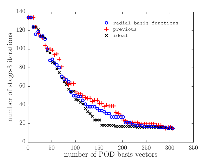
    Radial-basis-function weights. Noting that 𝐙j𝜼j=𝐏𝐀j𝒵j(𝐱j𝐱¯j)subscript𝐙𝑗subscriptsuperscript𝜼𝑗subscriptsuperscript𝐏subscript𝒵𝑗subscript𝐀𝑗superscriptsubscript𝐱𝑗subscript¯𝐱𝑗\mathbf{Z}_{j}\boldsymbol{\eta}^{\star}_{j}=\mathbf{P}^{\mathcal{Z}_{j}}_{{\mathbf{A}}_{j}}\left({{\mathbf{x}}_{j}^{\star}-\bar{\mathbf{x}}_{j}}\right), we can approximate ideal weights 𝜼jsubscriptsuperscript𝜼𝑗\boldsymbol{\eta}^{\star}_{j} by approximating the component of 𝐱j𝐱¯jsuperscriptsubscript𝐱𝑗subscript¯𝐱𝑗{\mathbf{x}}_{j}^{\star}-\bar{\mathbf{x}}_{j} in 𝒵jsubscript𝒵𝑗{\mathcal{Z}_{j}}. To achieve this, we assume the j𝑗jth solution can be approximated as a linear combination of previous solutions, i.e.,

    (39) 𝐏𝐀j𝒵j(𝐱j𝐱¯j)i=1ωρRBF(j,ji)(𝐏𝐀ji𝒵ji(𝐱ji𝐱¯ji)),subscriptsuperscript𝐏subscript𝒵𝑗subscript𝐀𝑗superscriptsubscript𝐱𝑗subscript¯𝐱𝑗superscriptsubscript𝑖1𝜔superscript𝜌RBF𝑗𝑗𝑖subscriptsuperscript𝐏subscript𝒵𝑗𝑖subscript𝐀𝑗𝑖subscriptsuperscript𝐱𝑗𝑖subscript¯𝐱𝑗𝑖\mathbf{P}^{\mathcal{Z}_{j}}_{{\mathbf{A}}_{j}}\left({{\mathbf{x}}_{j}^{\star}-\bar{\mathbf{x}}_{j}}\right)\approx\sum_{i=1}^{\omega}\rho^{\text{RBF}}(j,j-i)(\mathbf{P}^{\mathcal{Z}_{j-i}}_{{\mathbf{A}}_{j-i}}\left({{\mathbf{x}}^{\star}_{j-i}-\bar{\mathbf{x}}_{j-i}}\right)),

    where ωNaturej1𝜔Nature𝑗1\omega\in{\rm Nature}{j-1} denotes the number of previous solutions to include and ρRBF(i,j)superscript𝜌RBF𝑖𝑗\rho^{\text{RBF}}(i,j) denotes a radial basis function. This implies weights of

    (40) 𝜼jRBF(ω)=i=1ωρRBF(j,ji)(𝐙j+1iT𝐀ji𝐙j+1i)1𝐙j+1iT𝐀ji(𝐱ji𝐱¯ji)=i=1ωρRBF(j,ji)𝜼j+1iprev.subscriptsuperscript𝜼RBF𝑗𝜔superscriptsubscript𝑖1𝜔superscript𝜌RBF𝑗𝑗𝑖superscriptsuperscriptsubscript𝐙𝑗1𝑖𝑇subscript𝐀𝑗𝑖subscript𝐙𝑗1𝑖1superscriptsubscript𝐙𝑗1𝑖𝑇subscript𝐀𝑗𝑖subscriptsuperscript𝐱𝑗𝑖subscript¯𝐱𝑗𝑖superscriptsubscript𝑖1𝜔superscript𝜌RBF𝑗𝑗𝑖subscriptsuperscript𝜼prev𝑗1𝑖\displaystyle\begin{split}\boldsymbol{\eta}^{\text{RBF}}_{j}(\omega)&=\sum_{i=1}^{\omega}\rho^{\text{RBF}}(j,j-i)\left(\mathbf{Z}_{j+1-i}^{T}{\mathbf{A}}_{j-i}\mathbf{Z}_{j+1-i}\right)^{-1}\mathbf{Z}_{j+1-i}^{T}{\mathbf{A}}_{j-i}\left({\mathbf{x}}^{\star}_{j-i}-\bar{\mathbf{x}}_{j-i}\right)\\ &=\sum_{i=1}^{\omega}\rho^{\text{RBF}}(j,j-i)\boldsymbol{\eta}^{\text{prev}}_{j+1-i}.\end{split}

    In practice, we employ a inverse-distance-weight radial basis function of the form ρRBF(i,j)=ρIDW(|ij|)superscript𝜌RBF𝑖𝑗superscript𝜌IDW𝑖𝑗\rho^{\text{RBF}}(i,j)=\rho^{\text{IDW}}(|i-j|) with ρIDW:r1/2r1:superscript𝜌IDWmaps-to𝑟1superscript2𝑟1\rho^{\text{IDW}}:r\mapsto 1/2^{r-1}; we set ω𝜔\omega to be the number of linear systems since the most recent truncation.

3.3.3 Metric

Theorems 1 and 2 demonstrate that POD minimizes an upper bound for the errors 𝐱j𝐏𝐀j𝐱¯j+𝒴j(𝐱j)𝐀jsubscriptnormsuperscriptsubscript𝐱𝑗subscriptsuperscript𝐏subscript¯𝐱𝑗subscript𝒴𝑗subscript𝐀𝑗superscriptsubscript𝐱𝑗subscript𝐀𝑗\left\|{\mathbf{x}}_{j}^{\star}-\mathbf{P}^{\bar{\mathbf{x}}_{j}+\mathcal{Y}_{j}}_{{\mathbf{A}}_{j}}\left({{\mathbf{x}}_{j}^{\star}}\right)\right\|_{{\mathbf{A}}_{j}} and 𝐪(𝐱j)𝐪(𝐏𝐀j𝐱¯j+𝒴j(𝐱j))2subscriptnorm𝐪superscriptsubscript𝐱𝑗𝐪subscriptsuperscript𝐏subscript¯𝐱𝑗subscript𝒴𝑗subscript𝐀𝑗superscriptsubscript𝐱𝑗2\|{\mathbf{q}}\left({\mathbf{x}}_{j}^{\star}\right)-{\mathbf{q}}\left(\mathbf{P}^{\bar{\mathbf{x}}_{j}+\mathcal{Y}_{j}}_{{\mathbf{A}}_{j}}\left({{\mathbf{x}}_{j}^{\star}}\right)\right)\|_{2} only if POD metrics of 𝚯=𝐀j𝚯subscript𝐀𝑗{\boldsymbol{\Theta}}={\mathbf{A}}_{j} and 𝚯=𝐂T𝐂𝚯superscript𝐂𝑇𝐂{\boldsymbol{\Theta}}={\mathbf{C}}^{T}{\mathbf{C}} are used, respectively. However, as previously discussed, we aim to avoid using 𝐀jsubscript𝐀𝑗{\mathbf{A}}_{j} to truncate the basis 𝐙jsubscript𝐙𝑗\mathbf{Z}_{j}, as it entails reduced computations with the j𝑗jth linear system (i.e., solving Eqs. (17) with 𝐘j=𝐙jsubscript𝐘𝑗subscript𝐙𝑗\mathbf{Y}_{j}=\mathbf{Z}_{j}). Therefore, we employ two practical choices for metrics in Eq. (33):

  1. 1.

    𝚯=𝐀j1𝚯subscript𝐀𝑗1{\boldsymbol{\Theta}}={\mathbf{A}}_{j-1}. This approach aligns the truncation with minimizing 𝐱j𝐏𝐀j𝐱¯j+𝒴j(𝐱j)𝐀jsubscriptnormsuperscriptsubscript𝐱𝑗subscriptsuperscript𝐏subscript¯𝐱𝑗subscript𝒴𝑗subscript𝐀𝑗superscriptsubscript𝐱𝑗subscript𝐀𝑗\left\|{\mathbf{x}}_{j}^{\star}-\mathbf{P}^{\bar{\mathbf{x}}_{j}+\mathcal{Y}_{j}}_{{\mathbf{A}}_{j}}\left({{\mathbf{x}}_{j}^{\star}}\right)\right\|_{{\mathbf{A}}_{j}}. From Eq. (32), the resulting basis is 𝐀j1subscript𝐀𝑗1{\mathbf{A}}_{j-1}-orthogonal. Here, computing the POD basis via Algorithm 4 is appropriate, as a symmetric factorization of 𝐀j1subscript𝐀𝑗1{\mathbf{A}}_{j-1} is not readily available.

  2. 2.

    𝚯=𝐂T𝐂𝚯superscript𝐂𝑇𝐂{\boldsymbol{\Theta}}={\mathbf{C}}^{T}{\mathbf{C}}. This is an output-oriented approach associated with minimizing the output error. From Eq. (32), the resulting basis is 𝐂T𝐂superscript𝐂𝑇𝐂{\mathbf{C}}^{T}{\mathbf{C}}-orthogonal. Computing this POD basis via Algorithm 5 is appropriate, as a symmetric factor of the (pseudo)metric is readily available as 𝐂𝐂{\mathbf{C}}.

3.3.4 Computable goal-oriented POD methods

In summary, the four (computable) goal-oriented POD truncation methods we propose are

  1. 1.

    𝐘j=𝐔yj𝐀j1(𝐙j,𝜼jprev)subscript𝐘𝑗subscriptsuperscript𝐔subscript𝐀𝑗1subscript𝑦𝑗subscript𝐙𝑗subscriptsuperscript𝜼prev𝑗\mathbf{Y}_{j}={\mathbf{U}}^{{\mathbf{A}}_{j-1}}_{{y_{j}}}\left(\mathbf{Z}_{j},\boldsymbol{\eta}^{\text{prev}}_{j}\right), computable by (𝐘j)=pod_evd(𝐙j,𝜼jprev,𝐀j1,εy)subscript𝐘𝑗pod_evdsubscript𝐙𝑗subscriptsuperscript𝜼prev𝑗subscript𝐀𝑗1subscript𝜀𝑦(\mathbf{Y}_{j})=\texttt{pod\_evd}(\mathbf{Z}_{j},\boldsymbol{\eta}^{\text{prev}}_{j},{\mathbf{A}}_{j-1},\varepsilon_{y}),

  2. 2.

    𝐘j=𝐔yj𝐀j1(𝐙j,𝜼jRBF(ω))subscript𝐘𝑗subscriptsuperscript𝐔subscript𝐀𝑗1subscript𝑦𝑗subscript𝐙𝑗subscriptsuperscript𝜼RBF𝑗𝜔\mathbf{Y}_{j}={\mathbf{U}}^{{\mathbf{A}}_{j-1}}_{{y_{j}}}\left(\mathbf{Z}_{j},\boldsymbol{\eta}^{\text{RBF}}_{j}(\omega)\right), computable by (𝐘j)=pod_evd(𝐙j,𝜼jRBF(ω),𝐀j1,εy)subscript𝐘𝑗pod_evdsubscript𝐙𝑗subscriptsuperscript𝜼RBF𝑗𝜔subscript𝐀𝑗1subscript𝜀𝑦(\mathbf{Y}_{j})=\texttt{pod\_evd}(\mathbf{Z}_{j},\boldsymbol{\eta}^{\text{RBF}}_{j}(\omega),{\mathbf{A}}_{j-1},\varepsilon_{y}),

  3. 3.

    𝐘j=𝐔yj𝐂T𝐂(𝐙j,𝜼jprev)subscript𝐘𝑗subscriptsuperscript𝐔superscript𝐂𝑇𝐂subscript𝑦𝑗subscript𝐙𝑗subscriptsuperscript𝜼prev𝑗\mathbf{Y}_{j}={\mathbf{U}}^{{\mathbf{C}}^{T}{\mathbf{C}}}_{{y_{j}}}\left(\mathbf{Z}_{j},\boldsymbol{\eta}^{\text{prev}}_{j}\right), computable by (𝐘j)=pod_svd(𝐙j,𝜼jprev,𝐂,εy)subscript𝐘𝑗pod_svdsubscript𝐙𝑗subscriptsuperscript𝜼prev𝑗𝐂subscript𝜀𝑦(\mathbf{Y}_{j})=\texttt{pod\_svd}(\mathbf{Z}_{j},\boldsymbol{\eta}^{\text{prev}}_{j},{\mathbf{C}},\varepsilon_{y}),

  4. 4.

    𝐘j=𝐔yj𝐂T𝐂(𝐙j,𝜼jRBF(ω))subscript𝐘𝑗subscriptsuperscript𝐔superscript𝐂𝑇𝐂subscript𝑦𝑗subscript𝐙𝑗subscriptsuperscript𝜼RBF𝑗𝜔\mathbf{Y}_{j}={\mathbf{U}}^{{\mathbf{C}}^{T}{\mathbf{C}}}_{{y_{j}}}\left(\mathbf{Z}_{j},\boldsymbol{\eta}^{\text{RBF}}_{j}(\omega)\right), computable by (𝐘j)=pod_svd(𝐙j,𝜼jRBF(ω),𝐂,εy)subscript𝐘𝑗pod_svdsubscript𝐙𝑗subscriptsuperscript𝜼RBF𝑗𝜔𝐂subscript𝜀𝑦(\mathbf{Y}_{j})=\texttt{pod\_svd}(\mathbf{Z}_{j},\boldsymbol{\eta}^{\text{RBF}}_{j}(\omega),{\mathbf{C}},\varepsilon_{y}),

where εy[0,1]subscript𝜀𝑦01\varepsilon_{y}\in\left[0,1\right] is a statistical ‘energy criterion’ used to truncate the POD basis, and pod_evd and pod_svd are described in Algorithms 4 and 5, respectively. We now provide a result that allows us to bound the distance between the four computable goal-oriented POD subspaces above and their ideal counterparts, which correspond to 𝒰yj𝐀j(𝐙j,𝜼j)subscriptsuperscript𝒰subscript𝐀𝑗subscript𝑦𝑗subscript𝐙𝑗subscriptsuperscript𝜼𝑗\mathcal{U}^{{\mathbf{A}}_{j}}_{{y_{j}}}\left(\mathbf{Z}_{j},\boldsymbol{\eta}^{\star}_{j}\right) for 12 and 𝒰yj𝐂T𝐂(𝐙j,𝜼¯j)subscriptsuperscript𝒰superscript𝐂𝑇𝐂subscript𝑦𝑗subscript𝐙𝑗subscriptsuperscript¯𝜼𝑗\mathcal{U}^{{\mathbf{C}}^{T}{\mathbf{C}}}_{{y_{j}}}\left(\mathbf{Z}_{j},\bar{\boldsymbol{\eta}}^{\star}_{j}\right) for 34 above.

Theorem 5 (Distance between goal-oriented POD subspaces).

The distance between two goal-oriented POD subspaces 𝒰a:=𝒰y𝚯a(𝐒,𝛄a)assignsuperscript𝒰𝑎subscriptsuperscript𝒰superscript𝚯𝑎𝑦𝐒superscript𝛄𝑎\mathcal{U}^{a}\vcentcolon=\mathcal{U}^{{\boldsymbol{\Theta}}^{a}}_{y}\left({\mathbf{S}},\boldsymbol{\gamma}^{a}\right) and 𝒰b:=𝒰y𝚯b(𝐒,𝛄b)assignsuperscript𝒰𝑏subscriptsuperscript𝒰superscript𝚯b𝑦𝐒superscript𝛄b\mathcal{U}^{b}\vcentcolon=\mathcal{U}^{{\boldsymbol{\Theta}}^{\text{b}}}_{y}\left({\mathbf{S}},\boldsymbol{\gamma}^{\text{b}}\right)—which are characterized by different metrics 𝚯aSPSD(n)superscript𝚯𝑎SPSD𝑛{\boldsymbol{\Theta}}^{a}\in\text{SPSD}(n) and 𝚯bSPSD(n)superscript𝚯𝑏SPSD𝑛{\boldsymbol{\Theta}}^{b}\in\text{SPSD}(n) with 𝚯a=𝚯b+𝚫superscript𝚯𝑎superscript𝚯𝑏𝚫{\boldsymbol{\Theta}}^{a}={\boldsymbol{\Theta}}^{b}+\boldsymbol{\Delta} and different snapshot weights 𝚪a:=diag(γ1a,,γsa)assignsuperscript𝚪𝑎diagsubscriptsuperscript𝛾𝑎1subscriptsuperscript𝛾𝑎𝑠\boldsymbol{\Gamma}^{a}\vcentcolon=\text{diag}\left(\gamma^{a}_{1},\ldots,\gamma^{a}_{s}\right) and 𝚪b:=diag(γ1b,,γsb)assignsuperscript𝚪𝑏diagsubscriptsuperscript𝛾b1subscriptsuperscript𝛾b𝑠\boldsymbol{\Gamma}^{b}\vcentcolon=\text{diag}\left(\gamma^{\text{b}}_{1},\ldots,\gamma^{\text{b}}_{s}\right) associated with snapshots 𝐒n×s𝐒superscript𝑛𝑠{\mathbf{S}}\in\mathbb{R}^{n\times s}—can be bounded as

(41) d(𝒰a,𝒰b)κ(𝐒𝚪a)κ([𝚪a]1𝚪b𝐕b)(\displaystyle d\left(\mathcal{U}^{a},\mathcal{U}^{b}\right)\leq\kappa({\mathbf{S}}\boldsymbol{\Gamma}^{a})\kappa([\boldsymbol{\Gamma}^{a}]^{-1}\boldsymbol{\Gamma}^{b}{\mathbf{V}}^{b})\Bigl{(} (𝚪b+𝚪a)(𝚪b𝚪a)[𝚪a]1𝐒T𝚯b𝐒𝚪a2subscriptnormsuperscript𝚪𝑏superscript𝚪𝑎superscript𝚪𝑏superscript𝚪𝑎superscriptdelimited-[]superscript𝚪𝑎1superscript𝐒𝑇superscript𝚯𝑏𝐒superscript𝚪𝑎2\displaystyle\|\left(\boldsymbol{\Gamma}^{b}+\boldsymbol{\Gamma}^{a}\right)\left(\boldsymbol{\Gamma}^{b}-\boldsymbol{\Gamma}^{a}\right)[\boldsymbol{\Gamma}^{a}]^{-1}{\mathbf{S}}^{T}{\boldsymbol{\Theta}}^{b}{\mathbf{S}}\boldsymbol{\Gamma}^{a}\|_{2}
(42) +𝚫2𝐒𝚪a22)/abssep(𝚲a,𝚲b)\displaystyle+\|\boldsymbol{\Delta}\|_{2}\|{\mathbf{S}}\boldsymbol{\Gamma}^{a}\|^{2}_{2}\Bigr{)}/\text{abssep}(\boldsymbol{\Lambda}^{a}_{\perp},{\boldsymbol{\Lambda}}^{b})

if the matrix 𝐒𝚪a𝐒superscript𝚪𝑎{\mathbf{S}}\boldsymbol{\Gamma}^{a} has full column rank. Here, d(𝒰,𝒱):=maxu𝒰,u=1minv𝒱uv=sin(θmax)assign𝑑𝒰𝒱subscriptformulae-sequence𝑢𝒰norm𝑢1subscript𝑣𝒱norm𝑢𝑣subscript𝜃maxd\left(\mathcal{U},\mathcal{V}\right)\vcentcolon=\max_{u\in\mathcal{U},\|u\|=1}{\min_{v\in\mathcal{V}}}\|u-v\|=\sin(\theta_{\text{max}}), where θmaxsubscript𝜃max\theta_{\text{max}} is the largest principal angle between 𝒰𝒰\mathcal{U} and 𝒱𝒱\mathcal{V}, κ(𝐀)𝜅𝐀\kappa({\mathbf{A}}) denotes the condition number of matrix 𝐀𝐀{\mathbf{A}}, and abssep(𝚲1,𝚲2):=min𝐙2=1𝚲1𝐙𝐙𝚲22assignabssepsubscript𝚲1subscript𝚲2subscriptsubscriptnorm𝐙21subscriptnormsubscript𝚲1𝐙𝐙subscript𝚲22\text{abssep}(\boldsymbol{\Lambda}_{1},\boldsymbol{\Lambda}_{2})\vcentcolon=\min_{\|\boldsymbol{Z}\|_{2}=1}\|\boldsymbol{\Lambda}_{1}\boldsymbol{Z}-\boldsymbol{Z}\boldsymbol{\Lambda}_{2}\|_{2} denotes the absolute separation between two spectra. In addition, 𝐕b𝒮y(s)superscript𝐕𝑏subscript𝒮𝑦superscript𝑠{\mathbf{V}}^{b}\in\mathcal{S}_{y}({\mathbb{R}^{s}}) and 𝚲by×ysuperscript𝚲𝑏superscript𝑦𝑦{\boldsymbol{\Lambda}}^{b}\in\mathbb{R}^{y\times y} denote the first y𝑦y eigenvectors and (diagonal matrix of) eigenvalues, respectively, of the matrix 𝚪b𝐒T𝚯b𝐒𝚪bsuperscript𝚪𝑏superscript𝐒𝑇superscript𝚯𝑏𝐒superscript𝚪𝑏\boldsymbol{\Gamma}^{b}{\mathbf{S}}^{T}{\boldsymbol{\Theta}}^{b}{\mathbf{S}}\boldsymbol{\Gamma}^{b}, assuming eigenvalues are ordered in descending magnitude. Similarly, 𝚲asubscriptsuperscript𝚲𝑎perpendicular-to\boldsymbol{\Lambda}^{a}_{\perp} denotes the diagonal matrix of eigenvalues associated with the orthogonal complement to the invariant subspace spanned by the first y𝑦y eigenvectors of 𝚪a𝐒T𝚯a𝐒𝚪asuperscript𝚪𝑎superscript𝐒𝑇superscript𝚯𝑎𝐒superscript𝚪𝑎\boldsymbol{\Gamma}^{a}{\mathbf{S}}^{T}{\boldsymbol{\Theta}}^{a}{\mathbf{S}}\boldsymbol{\Gamma}^{a}.

This theorem allows us to bound the distances between the four computable POD subspaces and their ideal counterparts by substituting the appropriate quantities into Theorem 5. That is, the theorem allows us to bound the following quantities:

  1. 1.

    d(𝒰y𝐀j1(𝐙j,𝜼jprev),𝒰y𝐀j(𝐙j,𝜼j))𝑑subscriptsuperscript𝒰subscript𝐀𝑗1𝑦subscript𝐙𝑗subscriptsuperscript𝜼prev𝑗subscriptsuperscript𝒰subscript𝐀𝑗𝑦subscript𝐙𝑗subscriptsuperscript𝜼𝑗d\left(\mathcal{U}^{{\mathbf{A}}_{j-1}}_{y}\left(\mathbf{Z}_{j},\boldsymbol{\eta}^{\text{prev}}_{j}\right),\mathcal{U}^{{\mathbf{A}}_{j}}_{y}\left(\mathbf{Z}_{j},\boldsymbol{\eta}^{\star}_{j}\right)\right),

  2. 2.

    d(𝒰y𝐀j1(𝐙j,𝜼jRBF(ω)),𝒰y𝐀j(𝐙j,𝜼j))𝑑subscriptsuperscript𝒰subscript𝐀𝑗1𝑦subscript𝐙𝑗subscriptsuperscript𝜼RBF𝑗𝜔subscriptsuperscript𝒰subscript𝐀𝑗𝑦subscript𝐙𝑗subscriptsuperscript𝜼𝑗d\left(\mathcal{U}^{{\mathbf{A}}_{j-1}}_{y}\left(\mathbf{Z}_{j},\boldsymbol{\eta}^{\text{RBF}}_{j}(\omega)\right),\mathcal{U}^{{\mathbf{A}}_{j}}_{y}\left(\mathbf{Z}_{j},\boldsymbol{\eta}^{\star}_{j}\right)\right),

  3. 3.

    d(𝒰y𝐂T𝐂(𝐙j,𝜼jprev),𝒰y𝐂T𝐂(𝐙j,𝜼j))𝑑subscriptsuperscript𝒰superscript𝐂𝑇𝐂𝑦subscript𝐙𝑗subscriptsuperscript𝜼prev𝑗subscriptsuperscript𝒰superscript𝐂𝑇𝐂𝑦subscript𝐙𝑗subscriptsuperscript𝜼𝑗d\left(\mathcal{U}^{{\mathbf{C}}^{T}{\mathbf{C}}}_{y}\left(\mathbf{Z}_{j},\boldsymbol{\eta}^{\text{prev}}_{j}\right),\mathcal{U}^{{\mathbf{C}}^{T}{\mathbf{C}}}_{y}\left(\mathbf{Z}_{j},\boldsymbol{\eta}^{\star}_{j}\right)\right), and

  4. 4.

    d(𝒰y𝐂T𝐂(𝐙j,𝜼jRBF(ω)),𝒰y𝐂T𝐂(𝐙j,𝜼j))𝑑subscriptsuperscript𝒰superscript𝐂𝑇𝐂𝑦subscript𝐙𝑗subscriptsuperscript𝜼RBF𝑗𝜔subscriptsuperscript𝒰superscript𝐂𝑇𝐂𝑦subscript𝐙𝑗subscriptsuperscript𝜼𝑗d\left(\mathcal{U}^{{\mathbf{C}}^{T}{\mathbf{C}}}_{y}\left(\mathbf{Z}_{j},\boldsymbol{\eta}^{\text{RBF}}_{j}(\omega)\right),\mathcal{U}^{{\mathbf{C}}^{T}{\mathbf{C}}}_{y}\left(\mathbf{Z}_{j},\boldsymbol{\eta}^{\star}_{j}\right)\right).

Remark 2.

The subspace-distance bound (41) simplifies under certain conditions.
Fixed snapshot weights. First, note that when the snapshot weights are identical but the metric differes, i.e., 𝚪b=𝚪asuperscript𝚪𝑏superscript𝚪𝑎\boldsymbol{\Gamma}^{b}=\boldsymbol{\Gamma}^{a}, the first term within parentheses vanishes and κ([𝚪a]1𝚪b𝐕b)=1𝜅superscriptdelimited-[]superscript𝚪𝑎1superscript𝚪𝑏superscript𝐕𝑏1\kappa([\boldsymbol{\Gamma}^{a}]^{-1}\boldsymbol{\Gamma}^{b}{\mathbf{V}}^{b})=1 due to symmetry of 𝐁bsuperscript𝐁𝑏\mathbf{B}^{b}, which yields

(43) d(𝒰a,𝒰b)κ(𝐒𝚪a)𝚫2𝐒𝚪a22/abssep(𝚲a,𝚲b).𝑑superscript𝒰𝑎superscript𝒰𝑏𝜅𝐒superscript𝚪𝑎subscriptnorm𝚫2subscriptsuperscriptnorm𝐒superscript𝚪𝑎22abssepsubscriptsuperscript𝚲𝑎perpendicular-tosuperscript𝚲𝑏\displaystyle d\left(\mathcal{U}^{a},\mathcal{U}^{b}\right)\leq\kappa({\mathbf{S}}\boldsymbol{\Gamma}^{a})\|\boldsymbol{\Delta}\|_{2}\|{\mathbf{S}}\boldsymbol{\Gamma}^{a}\|^{2}_{2}/\text{abssep}(\boldsymbol{\Lambda}^{a}_{\perp},{\boldsymbol{\Lambda}}^{b}).

Thus, the subspace distance depends linearly on the norm of the metric perturbation in this case.

Fixed metric. If instead the snapshot weights differ while 𝚫=𝟎𝚫0\boldsymbol{\Delta}={\bf 0}, then the second term within parentheses vanishes and we have

(44) d(𝒰a,𝒰b)κ(𝐒𝚪a)κ([𝚪a]1𝚪b𝐕b)𝑑superscript𝒰𝑎superscript𝒰𝑏𝜅𝐒superscript𝚪𝑎𝜅superscriptdelimited-[]superscript𝚪𝑎1superscript𝚪𝑏superscript𝐕𝑏\displaystyle d\left(\mathcal{U}^{a},\mathcal{U}^{b}\right)\leq\kappa({\mathbf{S}}\boldsymbol{\Gamma}^{a})\kappa([\boldsymbol{\Gamma}^{a}]^{-1}\boldsymbol{\Gamma}^{b}{\mathbf{V}}^{b}) (𝚪b+𝚪a)(𝚪b𝚪a)[𝚪a]1𝐒T𝚯b𝐒𝚪a2/abssep(𝚲a,𝚲b)subscriptnormsuperscript𝚪𝑏superscript𝚪𝑎superscript𝚪𝑏superscript𝚪𝑎superscriptdelimited-[]superscript𝚪𝑎1superscript𝐒𝑇superscript𝚯𝑏𝐒superscript𝚪𝑎2abssepsubscriptsuperscript𝚲𝑎perpendicular-tosuperscript𝚲𝑏\displaystyle\|\left(\boldsymbol{\Gamma}^{b}+\boldsymbol{\Gamma}^{a}\right)\left(\boldsymbol{\Gamma}^{b}-\boldsymbol{\Gamma}^{a}\right)[\boldsymbol{\Gamma}^{a}]^{-1}{\mathbf{S}}^{T}{\boldsymbol{\Theta}}^{b}{\mathbf{S}}\boldsymbol{\Gamma}^{a}\|_{2}/\text{abssep}(\boldsymbol{\Lambda}^{a}_{\perp},{\boldsymbol{\Lambda}}^{b})

In practice, this situation corresponds to cases 34 above (where 𝚯b=𝚯a=𝐂T𝐂superscript𝚯𝑏superscript𝚯𝑎superscript𝐂𝑇𝐂{\boldsymbol{\Theta}}^{b}={\boldsymbol{\Theta}}^{a}={\mathbf{C}}^{T}{\mathbf{C}}) or to cases 12 when 𝐀j=𝐀j1subscript𝐀𝑗subscript𝐀𝑗1{\mathbf{A}}_{j}={\mathbf{A}}_{j-1}. Notice that the relative weight perturbation (𝚪b𝚪a)[𝚪a]1superscript𝚪𝑏superscript𝚪𝑎superscriptdelimited-[]superscript𝚪𝑎1(\boldsymbol{\Gamma}^{b}-\boldsymbol{\Gamma}^{a})[\boldsymbol{\Gamma}^{a}]^{-1} appears within the remaining term. When the relative weight perturbation can be bounded as

maxk(𝜸jb𝜸a)k/(𝜸a)kδ^,\max_{k}{(\boldsymbol{\gamma}^{b}_{j}-\boldsymbol{\gamma}^{a})_{k}/(\boldsymbol{\gamma}^{a})_{k}}\leq\hat{\delta},

then it can be shown that the bound simplifies to

(45) d(𝒰a,𝒰b)κ(𝐒𝚪a)κ([𝚪a]1𝚪b𝐕b)𝑑superscript𝒰𝑎superscript𝒰𝑏𝜅𝐒superscript𝚪𝑎𝜅superscriptdelimited-[]superscript𝚪𝑎1superscript𝚪𝑏superscript𝐕𝑏\displaystyle d\left(\mathcal{U}^{a},\mathcal{U}^{b}\right)\leq\kappa({\mathbf{S}}\boldsymbol{\Gamma}^{a})\kappa([\boldsymbol{\Gamma}^{a}]^{-1}\boldsymbol{\Gamma}^{b}{\mathbf{V}}^{b}) δ^(2+δ^)𝚪a𝐒T𝚯a𝐒𝚪a2/abssep(𝚲a,𝚲b).^𝛿2^𝛿subscriptnormsuperscript𝚪𝑎superscript𝐒𝑇superscript𝚯𝑎𝐒superscript𝚪𝑎2abssepsubscriptsuperscript𝚲𝑎perpendicular-tosuperscript𝚲𝑏\displaystyle\hat{\delta}(2+\hat{\delta})\|\boldsymbol{\Gamma}^{a}{\mathbf{S}}^{T}{\boldsymbol{\Theta}}^{a}{\mathbf{S}}\boldsymbol{\Gamma}^{a}\|_{2}/\text{abssep}(\boldsymbol{\Lambda}^{a}_{\perp},{\boldsymbol{\Lambda}}^{b}).

Further, when 𝚪asuperscript𝚪𝑎\boldsymbol{\Gamma}^{a} commutes with 𝐒T𝚯b𝐒superscript𝐒𝑇superscript𝚯𝑏𝐒{\mathbf{S}}^{T}{\boldsymbol{\Theta}}^{b}{\mathbf{S}}, then the bound simplifies to

(46) d(𝒰a,𝒰b)κ(𝐒𝚪a)κ([𝚪a]1𝚪b𝐕b)𝑑superscript𝒰𝑎superscript𝒰𝑏𝜅𝐒superscript𝚪𝑎𝜅superscriptdelimited-[]superscript𝚪𝑎1superscript𝚪𝑏superscript𝐕𝑏\displaystyle d\left(\mathcal{U}^{a},\mathcal{U}^{b}\right)\leq\kappa({\mathbf{S}}\boldsymbol{\Gamma}^{a})\kappa([\boldsymbol{\Gamma}^{a}]^{-1}\boldsymbol{\Gamma}^{b}{\mathbf{V}}^{b}) (𝚪b+𝚪a)(𝚪b𝚪a)𝐒T𝚯b𝐒2/abssep(𝚲a,𝚲b),subscriptnormsuperscript𝚪𝑏superscript𝚪𝑎superscript𝚪𝑏superscript𝚪𝑎superscript𝐒𝑇superscript𝚯𝑏𝐒2abssepsubscriptsuperscript𝚲𝑎perpendicular-tosuperscript𝚲𝑏\displaystyle\|\left(\boldsymbol{\Gamma}^{b}+\boldsymbol{\Gamma}^{a}\right)\left(\boldsymbol{\Gamma}^{b}-\boldsymbol{\Gamma}^{a}\right){\mathbf{S}}^{T}{\boldsymbol{\Theta}}^{b}{\mathbf{S}}\|_{2}/\text{abssep}(\boldsymbol{\Lambda}^{a}_{\perp},{\boldsymbol{\Lambda}}^{b}),

which now depends on the absolute weight perturbation, 𝚪b𝚪asuperscript𝚪𝑏superscript𝚪𝑎\boldsymbol{\Gamma}^{b}-\boldsymbol{\Gamma}^{a}, rather than a relative perturbation. This occurs for cases 12 above when 𝐀1==𝐀j=𝐀subscript𝐀1subscript𝐀𝑗𝐀{\mathbf{A}}_{1}=\cdots={\mathbf{A}}_{j}={\mathbf{A}} (i.e., an invariant matrix), as 𝐒T𝚯b𝐒superscript𝐒𝑇superscript𝚯𝑏𝐒{\mathbf{S}}^{T}{\boldsymbol{\Theta}}^{b}{\mathbf{S}} is diagonal due to enforced 𝐀𝐀{\mathbf{A}}-orthogonality of 𝐒𝐒{\mathbf{S}}.

Strongly separated eigenvalues. If the eigenvalues associated with 𝚲bsuperscript𝚲𝑏{\boldsymbol{\Lambda}}^{b} and 𝚲asubscriptsuperscript𝚲𝑎perpendicular-to\boldsymbol{\Lambda}^{a}_{\perp} in Theorem 5 are strongly separated, i.e.,

0<δa:=max{minλ𝚲b|λ|maxλ^𝚲a|λ^|,minλ^𝚲a|λ^|maxλ𝚲b|λ|}0subscript𝛿𝑎assignsubscript𝜆superscript𝚲𝑏𝜆subscript^𝜆subscriptsuperscript𝚲𝑎perpendicular-to^𝜆subscript^𝜆subscriptsuperscript𝚲𝑎perpendicular-to^𝜆subscript𝜆superscript𝚲𝑏𝜆0<\delta_{a}\vcentcolon=\max\{\min_{\lambda\in{\boldsymbol{\Lambda}}^{b}}|\lambda|-\max_{\hat{\lambda}\in\boldsymbol{\Lambda}^{a}_{\perp}}|\hat{\lambda}|,\min_{\hat{\lambda}\in\boldsymbol{\Lambda}^{a}_{\perp}}|\hat{\lambda}|-\max_{\lambda\in{\boldsymbol{\Lambda}}^{b}}|\lambda|\}

then the expression for the subspace-distance bound becomes [19, Theorem 5.3]

(47) d(𝒰a,𝒰b)κ(𝐒𝚪a)κ([𝚪a]1𝚪b𝐕b)(\displaystyle d\left(\mathcal{U}^{a},\mathcal{U}^{b}\right)\leq\kappa({\mathbf{S}}\boldsymbol{\Gamma}^{a})\kappa([\boldsymbol{\Gamma}^{a}]^{-1}\boldsymbol{\Gamma}^{b}{\mathbf{V}}^{b})\Bigl{(} (𝚪b+𝚪a)(𝚪b𝚪a)[𝚪a]1𝐒T𝚯b𝐒𝚪a2subscriptnormsuperscript𝚪𝑏superscript𝚪𝑎superscript𝚪𝑏superscript𝚪𝑎superscriptdelimited-[]superscript𝚪𝑎1superscript𝐒𝑇superscript𝚯𝑏𝐒superscript𝚪𝑎2\displaystyle\|\left(\boldsymbol{\Gamma}^{b}+\boldsymbol{\Gamma}^{a}\right)\left(\boldsymbol{\Gamma}^{b}-\boldsymbol{\Gamma}^{a}\right)[\boldsymbol{\Gamma}^{a}]^{-1}{\mathbf{S}}^{T}{\boldsymbol{\Theta}}^{b}{\mathbf{S}}\boldsymbol{\Gamma}^{a}\|_{2}
(48) +𝚫2𝐒𝚪a22)/δa.\displaystyle+\|\boldsymbol{\Delta}\|_{2}\|{\mathbf{S}}\boldsymbol{\Gamma}^{a}\|^{2}_{2}\Bigr{)}/\delta_{a}.

Finally, we note that we can apply the results in Eq. (37) from Theorem 3 to those of Theorem 5 via the triangle inequality to obtain a more explicit subspace-distance bound for case 1 above, where 𝚪a=diag([𝛈j]1,,[𝛈j]s)superscript𝚪𝑎diagsubscriptdelimited-[]subscriptsuperscript𝛈𝑗1subscriptdelimited-[]subscriptsuperscript𝛈𝑗𝑠\boldsymbol{\Gamma}^{a}=\text{diag}\left([\boldsymbol{\eta}^{\star}_{j}]_{1},\ldots,[\boldsymbol{\eta}^{\star}_{j}]_{s}\right) and 𝚪b=diag([𝛈jprev]1,,[𝛈jprev]s)superscript𝚪𝑏diagsubscriptdelimited-[]subscriptsuperscript𝛈prev𝑗1subscriptdelimited-[]subscriptsuperscript𝛈prev𝑗𝑠\boldsymbol{\Gamma}^{b}=\text{diag}\left([\boldsymbol{\eta}^{\text{prev}}_{j}]_{1},\ldots,[\boldsymbol{\eta}^{\text{prev}}_{j}]_{s}\right).

4 Three-stage algorithm

From Section 2.2, we know that augmented PCG relies on first computing a solution over the augmenting subspace 𝐱¯j+𝒴jsubscript¯𝐱𝑗subscript𝒴𝑗\bar{\mathbf{x}}_{j}+\mathcal{Y}_{j}. While this can be accomplished by solving the Galerkin system (17) directly, this requires assembling the reduced matrix 𝐘jT𝐀j𝐘jsuperscriptsubscript𝐘𝑗𝑇subscript𝐀𝑗subscript𝐘𝑗\mathbf{Y}_{j}^{T}{\mathbf{A}}_{j}\mathbf{Y}_{j}, which incurs yjsubscript𝑦𝑗{y_{j}} matrix–vector products and 𝒪((τj+yj)yjn)𝒪subscript𝜏𝑗subscript𝑦𝑗subscript𝑦𝑗𝑛\mathcal{O}((\tau_{j}+{y_{j}}){y_{j}}n) flops, where τjsubscript𝜏𝑗\tau_{j} denotes the average number of nonzeros per row of 𝐀jsubscript𝐀𝑗{\mathbf{A}}_{j} This cost can be significant when the dimension of the augmenting space yjsubscript𝑦𝑗{y_{j}} becomes large.

To mitigate this effect, we propose a novel three-stage algorithm for augmented PCG. The algorithm leverages an augmenting basis that is optimally ordered and yields a well-conditioned reduced matrix. In particular, for linear system j𝑗j, we assume that an augmenting basis 𝐘jn×yjsubscript𝐘𝑗superscriptsubscript𝑛subscript𝑦𝑗\mathbf{Y}_{j}\in\mathbb{R}_{\star}^{n\times{y_{j}}} is available that 1) contains a low-dimensional basis 𝐖jn×wjsubscript𝐖𝑗superscriptsubscript𝑛subscript𝑤𝑗\mathbf{W}_{j}\in\mathbb{R}_{\star}^{n\times w_{j}} with 𝒲j𝒴jnsubscript𝒲𝑗subscript𝒴𝑗superscript𝑛{\mathcal{W}_{j}}\subseteq{\mathcal{Y}_{j}}\subseteq\mathbb{R}^{n} and wjyjnsubscript𝑤𝑗subscript𝑦𝑗𝑛w_{j}\leq{y_{j}}\leq n that can capture an accurate solution, and 2) yields a well-conditioned reduced matrix 𝐘jT𝐀j𝐘jsuperscriptsubscript𝐘𝑗𝑇subscript𝐀𝑗subscript𝐘𝑗\mathbf{Y}_{j}^{T}{\mathbf{A}}_{j}\mathbf{Y}_{j}. Given this basis, stage 1 first computes an accurate solution over the subspace 𝐱¯j+𝒲jsubscript¯𝐱𝑗subscript𝒲𝑗\bar{\mathbf{x}}_{j}+\mathcal{W}_{j}; a direct approach is suitable due to its assumed low dimensionality. Stage 2 iteratively computes a solution over 𝐱¯j+𝒴jsubscript¯𝐱𝑗subscript𝒴𝑗\bar{\mathbf{x}}_{j}+\mathcal{Y}_{j}. This should be efficient, as 𝐘jT𝐀j𝐘jsuperscriptsubscript𝐘𝑗𝑇subscript𝐀𝑗subscript𝐘𝑗\mathbf{Y}_{j}^{T}{\mathbf{A}}_{j}\mathbf{Y}_{j} need never be formed: the well-conditioned assumption implies that a preconditioner is not required for fast convergence and matrix–vector products of the form 𝐘T𝐀𝐘𝐩superscript𝐘𝑇𝐀𝐘𝐩\mathbf{Y}^{T}{\mathbf{A}}\mathbf{Y}{\mathbf{p}} can be computed using a single matrix–vector product as 𝐘T(𝐀(𝐘𝐩))superscript𝐘𝑇𝐀𝐘𝐩\mathbf{Y}^{T}({\mathbf{A}}(\mathbf{Y}{\mathbf{p}})). Finally, stage 3 applies augmented PCG in the full space to compute a solution satisfying the specified tolerance ϵjsubscriptitalic-ϵ𝑗\epsilon_{j}.

Goal-oriented POD as proposed in Section 3.3 fits naturally into this framework. First, the basis vectors are optimally ordered (Remark 1): the first few POD basis vectors span an optimal subspace in the sense of minimizing the objective function in Eq. (28), which is an upper bound for the 𝐀jsubscript𝐀𝑗{\mathbf{A}}_{j}-norm and 𝐂T𝐂superscript𝐂𝑇𝐂{\mathbf{C}}^{T}{\mathbf{C}}-norm of the error, respectively (Theorems 1 and 2). This implies that the first few POD vectors could be employed as 𝐖jsubscript𝐖𝑗\mathbf{W}_{j}. Second, it automatically yields a well-conditioned reduced matrix if 𝚯=𝐀j𝚯subscript𝐀𝑗{\boldsymbol{\Theta}}={\mathbf{A}}_{j}; this will be further discussed in Section 4.4.1. However, other truncation methods that satisfy these properties can also be considered within the proposed three-stage algorithm.

4.1 Stage 1

The objective of Stage 1 is to ‘jump start’ the algorithm by computing an accurate solution at very low cost. To achieve this, this stage computes 𝐱¯j+𝐖j𝐰^j=𝐏𝐀j𝐱¯j+𝒲j(𝐱j)subscript¯𝐱𝑗subscript𝐖𝑗subscript^𝐰𝑗subscriptsuperscript𝐏subscript¯𝐱𝑗subscript𝒲𝑗subscript𝐀𝑗superscriptsubscript𝐱𝑗\bar{\mathbf{x}}_{j}+\mathbf{W}_{j}\hat{\mathbf{w}}_{j}=\mathbf{P}^{\bar{\mathbf{x}}_{j}+{\mathcal{W}_{j}}}_{{\mathbf{A}}_{j}}\left({{\mathbf{x}}_{j}^{\star}}\right) by solving

(49) 𝐖jT𝐀j𝐖j𝐰^j=𝐖jT(𝐛j𝐀j𝐱¯j)superscriptsubscript𝐖𝑗𝑇subscript𝐀𝑗subscript𝐖𝑗subscript^𝐰𝑗superscriptsubscript𝐖𝑗𝑇subscript𝐛𝑗subscript𝐀𝑗subscript¯𝐱𝑗\mathbf{W}_{j}^{T}{\mathbf{A}}_{j}\mathbf{W}_{j}\hat{\mathbf{w}}_{j}=\mathbf{W}_{j}^{T}({\mathbf{b}}_{j}-{\mathbf{A}}_{j}\bar{\mathbf{x}}_{j})

directly. The assumptions placed on 𝐖jsubscript𝐖𝑗\mathbf{W}_{j} imply that the solution 𝐱¯j+𝐖j𝐰^jsubscript¯𝐱𝑗subscript𝐖𝑗subscript^𝐰𝑗\bar{\mathbf{x}}_{j}+\mathbf{W}_{j}\hat{\mathbf{w}}_{j} will be accurate and a direct solve will be inexpensive. Computing this solution can be executed via Algorithm 2 as

(𝐰^j,𝐑^j)=direct_reduced_solve(𝐀j,𝐛j𝐀j𝐱¯j,𝐖j).subscript^𝐰𝑗subscript^𝐑𝑗direct_reduced_solvesubscript𝐀𝑗subscript𝐛𝑗subscript𝐀𝑗subscript¯𝐱𝑗subscript𝐖𝑗(\hat{\mathbf{w}}_{j},\hat{\bf R}_{j})=\texttt{direct\_reduced\_solve}({\mathbf{A}}_{j},{\mathbf{b}}_{j}-{\mathbf{A}}_{j}\bar{\mathbf{x}}_{j},\mathbf{W}_{j}).
Algorithm 2 direct_reduced_solve
0:  𝐀𝐀{\mathbf{A}}, 𝐛𝐛{\mathbf{b}}, 𝐖𝐖\mathbf{W}
0:  𝐰^^𝐰\hat{\mathbf{w}}, 𝐑^^𝐑\hat{\bf R}
1:  Compute 𝐀^=𝐖T𝐀𝐖^𝐀superscript𝐖𝑇𝐀𝐖\hat{\mathbf{A}}=\mathbf{W}^{T}{\mathbf{A}}\mathbf{W} and 𝐛^=𝐖T𝐛^𝐛superscript𝐖𝑇𝐛\hat{\mathbf{b}}=\mathbf{W}^{T}{\mathbf{b}}
2:  Solve 𝐀^𝐰^=𝐛^^𝐀^𝐰^𝐛\hat{\mathbf{A}}\hat{\mathbf{w}}=\hat{\mathbf{b}} by Cholesky factorization 𝐀^=𝐑^T𝐑^^𝐀superscript^𝐑𝑇^𝐑\hat{\mathbf{A}}=\hat{\bf R}^{T}\hat{\bf R}

4.2 Stage 2

The objective of Stage 2 is to improve upon the stage-1 solution 𝐱¯j+𝐖j𝐰^jsubscript¯𝐱𝑗subscript𝐖𝑗subscript^𝐰𝑗\bar{\mathbf{x}}_{j}+\mathbf{W}_{j}\hat{\mathbf{w}}_{j} by efficiently solving over the entire augmenting subspace 𝒴jsubscript𝒴𝑗{\mathcal{Y}_{j}}, whose dimension yjsubscript𝑦𝑗{y_{j}} may be large, while avoiding the cost of explicitly forming the reduced matrix 𝐘jT𝐀j𝐘jsuperscriptsubscript𝐘𝑗𝑇subscript𝐀𝑗subscript𝐘𝑗\mathbf{Y}_{j}^{T}{\mathbf{A}}_{j}\mathbf{Y}_{j}. To achieve this, this stage solves

(50) 𝐘jT𝐀j𝐘j𝐲^j=𝐘jT(𝐛j𝐀j𝐱¯j𝐀j𝐖j𝐰^j)superscriptsubscript𝐘𝑗𝑇subscript𝐀𝑗subscript𝐘𝑗superscriptsubscript^𝐲𝑗superscriptsubscript𝐘𝑗𝑇subscript𝐛𝑗subscript𝐀𝑗subscript¯𝐱𝑗subscript𝐀𝑗subscript𝐖𝑗subscript^𝐰𝑗\mathbf{Y}_{j}^{T}{\mathbf{A}}_{j}\mathbf{Y}_{j}\hat{{\mathbf{y}}}_{j}^{\star}=\mathbf{Y}_{j}^{T}\left({\mathbf{b}}_{j}-{\mathbf{A}}_{j}\bar{\mathbf{x}}_{j}-{\mathbf{A}}_{j}\mathbf{W}_{j}\hat{\mathbf{w}}_{j}\right)

iteratively to tolerance ϵ^jsubscript^italic-ϵ𝑗\hat{\epsilon}_{j} via augmented CG with augmenting basis 𝐖^jyj×wjsubscript^𝐖𝑗superscriptsubscriptsubscript𝑦𝑗subscript𝑤𝑗{\hat{\mathbf{W}}_{j}}\in\mathbb{R}_{\star}^{{y_{j}}\times w_{j}}, which represents the stage-1 basis in augmenting-subspace coordinates, i.e., 𝐖j=𝐘j𝐖^jsubscript𝐖𝑗subscript𝐘𝑗subscript^𝐖𝑗\mathbf{W}_{j}=\mathbf{Y}_{j}{\hat{\mathbf{W}}_{j}}. This approach is promising for two reasons. First, it precludes the need to explicitly compute the reduced matrix, as matrix–vector products of the form 𝐘jT𝐀j𝐘j𝐩superscriptsubscript𝐘𝑗𝑇subscript𝐀𝑗subscript𝐘𝑗𝐩\mathbf{Y}_{j}^{T}{\mathbf{A}}_{j}\mathbf{Y}_{j}{\mathbf{p}} can be computed via 𝐘jT(𝐀j(𝐘j𝐩))superscriptsubscript𝐘𝑗𝑇subscript𝐀𝑗subscript𝐘𝑗𝐩\mathbf{Y}_{j}^{T}({\mathbf{A}}_{j}(\mathbf{Y}_{j}{\mathbf{p}})) using a single matrix–vector product and 𝒪((2yj+τj)n)𝒪2subscript𝑦𝑗subscript𝜏𝑗𝑛\mathcal{O}((2{y_{j}}+\tau_{j})n) flops. Second, a small number of iterations will be needed for convergence if the reduced matrix 𝐘jT𝐀j𝐘jsuperscriptsubscript𝐘𝑗𝑇subscript𝐀𝑗subscript𝐘𝑗\mathbf{Y}_{j}^{T}{\mathbf{A}}_{j}\mathbf{Y}_{j} is well conditioned, as has been assumed.

Therefore, this stage amounts to executing Algorithm 1 as

(k^j,𝐱^j,𝐗^j,𝚪^j)=augmented_pcg(𝐘jT𝐀j𝐘j,𝐘jT(𝐛j𝐀j𝐱¯j),𝐰^j,𝐖^j,𝐈,ϵ^j)subscript^𝑘𝑗subscript^𝐱𝑗subscript^𝐗𝑗subscript^𝚪𝑗augmented_pcgsuperscriptsubscript𝐘𝑗𝑇subscript𝐀𝑗subscript𝐘𝑗superscriptsubscript𝐘𝑗𝑇subscript𝐛𝑗subscript𝐀𝑗subscript¯𝐱𝑗subscript^𝐰𝑗subscript^𝐖𝑗𝐈subscript^italic-ϵ𝑗(\hat{k}_{j},\hat{\mathbf{x}}_{j},{\hat{\mathbf{X}}}_{j},\hat{\boldsymbol{\Gamma}}_{j})=\texttt{augmented\_pcg}(\mathbf{Y}_{j}^{T}{\mathbf{A}}_{j}\mathbf{Y}_{j},\mathbf{Y}_{j}^{T}({\mathbf{b}}_{j}-{\mathbf{A}}_{j}\bar{\mathbf{x}}_{j}),\hat{\mathbf{w}}_{j},{\hat{\mathbf{W}}_{j}},\mathbf{I},\hat{\epsilon}_{j})

with an implementation optimization: the solves in steps 4 and 13 of Algorithm 1 can be performed directly in 𝒪(wj2)𝒪superscriptsubscript𝑤𝑗2\mathcal{O}(w_{j}^{2}) flops, as the Cholesky factorization of 𝐖jT𝐀j𝐖j=𝐑^jT𝐑^jsuperscriptsubscript𝐖𝑗𝑇subscript𝐀𝑗subscript𝐖𝑗superscriptsubscript^𝐑𝑗𝑇subscript^𝐑𝑗\mathbf{W}_{j}^{T}{\mathbf{A}}_{j}\mathbf{W}_{j}=\hat{\bf R}_{j}^{T}\hat{\bf R}_{j} can be reused from stage 1.

The (inexact) solution increment 𝐘j𝐲^j=𝐗j𝐱^jsubscript𝐘𝑗subscript^𝐲𝑗subscript𝐗𝑗subscript^𝐱𝑗\mathbf{Y}_{j}\hat{{\mathbf{y}}}_{j}=\mathbf{X}_{j}\hat{\mathbf{x}}_{j} computed by stage 2 lies in the range of a (reduced) Krylov basis 𝐗j=𝐘j𝐗^jn×k^jsubscript𝐗𝑗subscript𝐘𝑗subscript^𝐗𝑗superscript𝑛subscript^𝑘𝑗\mathbf{X}_{j}=\mathbf{Y}_{j}{\hat{\mathbf{X}}}_{j}\in\mathbb{R}^{n\times\hat{k}_{j}} with 𝒳j𝒴jnsubscript𝒳𝑗subscript𝒴𝑗superscript𝑛{\mathcal{X}_{j}}\subseteq{\mathcal{Y}_{j}}\subseteq\mathbb{R}^{n} and 𝐗^jyj×k^jsubscript^𝐗𝑗superscriptsubscript𝑦𝑗subscript^𝑘𝑗{\hat{\mathbf{X}}}_{j}\in\mathbb{R}^{{y_{j}}\times\hat{k}_{j}}, where k^jyjsubscript^𝑘𝑗subscript𝑦𝑗\hat{k}_{j}\leq{y_{j}} denotes the number of stage-2 iterations. This basis satisfies

(51) 𝐗jT𝐀j𝐗j=𝚪^j,𝐗jT𝐀j𝐖j=0,formulae-sequencesuperscriptsubscript𝐗𝑗𝑇subscript𝐀𝑗subscript𝐗𝑗subscript^𝚪𝑗superscriptsubscript𝐗𝑗𝑇subscript𝐀𝑗subscript𝐖𝑗0\displaystyle\mathbf{X}_{j}^{T}{\mathbf{A}}_{j}\mathbf{X}_{j}=\hat{\boldsymbol{\Gamma}}_{j},\quad\mathbf{X}_{j}^{T}{\mathbf{A}}_{j}\mathbf{W}_{j}=0,
(52) 𝒲j^𝒳^j=𝒲j^+K(k^j)(𝐘jT𝐀j𝐘j,𝐘jT(𝐛j𝐀j𝐱¯j𝐀j𝐖j𝐰^j)),direct-sum^subscript𝒲𝑗subscript^𝒳𝑗^subscript𝒲𝑗superscript𝐾subscript^𝑘𝑗superscriptsubscript𝐘𝑗𝑇subscript𝐀𝑗subscript𝐘𝑗superscriptsubscript𝐘𝑗𝑇subscript𝐛𝑗subscript𝐀𝑗subscript¯𝐱𝑗subscript𝐀𝑗subscript𝐖𝑗subscript^𝐰𝑗\displaystyle{{\hat{{\mathcal{W}}_{j}}}}\oplus{\hat{\mathcal{X}}_{j}}={\hat{{\mathcal{W}}_{j}}}+{K}^{(\hat{k}_{j})}\left(\mathbf{Y}_{j}^{T}{\mathbf{A}}_{j}\mathbf{Y}_{j},\mathbf{Y}_{j}^{T}({\mathbf{b}}_{j}-{\mathbf{A}}_{j}\bar{\mathbf{x}}_{j}-{\mathbf{A}}_{j}\mathbf{W}_{j}\hat{\mathbf{w}}_{j})\right),

while the resulting solution satisfies

(53) 𝐱¯j+𝐖j𝐰^j+𝐗j𝐱^jsubscript¯𝐱𝑗subscript𝐖𝑗subscript^𝐰𝑗subscript𝐗𝑗subscript^𝐱𝑗\displaystyle\bar{\mathbf{x}}_{j}+\mathbf{W}_{j}\hat{\mathbf{w}}_{j}+\mathbf{X}_{j}\hat{\mathbf{x}}_{j} =𝐏𝐀j𝐱¯j+𝒲j𝒳j(𝐱j)absentsubscriptsuperscript𝐏direct-sumsubscript¯𝐱𝑗subscript𝒲𝑗subscript𝒳𝑗subscript𝐀𝑗superscriptsubscript𝐱𝑗\displaystyle=\mathbf{P}^{\bar{\mathbf{x}}_{j}+{\mathcal{W}_{j}}\oplus{\mathcal{X}_{j}}}_{{\mathbf{A}}_{j}}\left({{\mathbf{x}}_{j}^{\star}}\right)

Ref. [33] proposed a similar idea referred to as the iterative reuse of Krylov subspaces (IRKS). This approach did not employ stage-1 direct solve and supported using either 𝐘j=[𝐕1𝐕j1]subscript𝐘𝑗delimited-[]subscript𝐕1subscript𝐕𝑗1\mathbf{Y}_{j}=\left[{\mathbf{V}}_{1}\ \cdots\ {\mathbf{V}}_{j-1}\right] or 𝐘j=𝐕j1subscript𝐘𝑗subscript𝐕𝑗1\mathbf{Y}_{j}={\mathbf{V}}_{j-1} (i.e., no truncation).

4.3 Stage 3

The objective of stage 3 is to continue iterating in the full space until the specified tolerance ϵjsubscriptitalic-ϵ𝑗\epsilon_{j} is satisfied. This stage therefore solves

(54) 𝐀jδ𝐱j=𝐛j𝐀j𝐱¯j𝐀j𝐖j𝐰^j𝐀j𝐗j𝐱^jsubscript𝐀𝑗𝛿superscriptsubscript𝐱𝑗subscript𝐛𝑗subscript𝐀𝑗subscript¯𝐱𝑗subscript𝐀𝑗subscript𝐖𝑗subscript^𝐰𝑗subscript𝐀𝑗subscript𝐗𝑗subscript^𝐱𝑗{\mathbf{A}}_{j}\delta\mathbf{x}_{j}^{\star}={\mathbf{b}}_{j}-{\mathbf{A}}_{j}\bar{\mathbf{x}}_{j}-{\mathbf{A}}_{j}\mathbf{W}_{j}\hat{\mathbf{w}}_{j}-{\mathbf{A}}_{j}\mathbf{X}_{j}\hat{\mathbf{x}}_{j}

via augmented PCG with augmenting basis [𝐖j,𝐗j]subscript𝐖𝑗subscript𝐗𝑗[\mathbf{W}_{j},\ \mathbf{X}_{j}]. Critically, note that the augmenting subspace used in stage 3 satisfies range([𝐖j,𝐗j])𝒴jrangesubscript𝐖𝑗subscript𝐗𝑗subscript𝒴𝑗\text{range}([\mathbf{W}_{j},\ \mathbf{X}_{j}])\subseteq\mathcal{Y}_{j}. This choice is made because 𝐀j[𝐖j,𝐗j]subscript𝐀𝑗subscript𝐖𝑗subscript𝐗𝑗{\mathbf{A}}_{j}[\mathbf{W}_{j},\ \mathbf{X}_{j}] and [𝐖j,𝐗j]T𝐀j[𝐖j,𝐗j]superscriptsubscript𝐖𝑗subscript𝐗𝑗𝑇subscript𝐀𝑗subscript𝐖𝑗subscript𝐗𝑗[\mathbf{W}_{j},\ \mathbf{X}_{j}]^{T}{\mathbf{A}}_{j}[\mathbf{W}_{j},\ \mathbf{X}_{j}]—which are required for orthogonalization in step 13 of Algorithm 1—are available from stages 1 and 2. Treating 𝒴jsubscript𝒴𝑗\mathcal{Y}_{j} as the augmenting subspace in stage 3 would necessitate computing 𝐀j𝐘jsubscript𝐀𝑗subscript𝐘𝑗{\mathbf{A}}_{j}\mathbf{Y}_{j} and 𝐘jT𝐀j𝐘jsuperscriptsubscript𝐘𝑗𝑇subscript𝐀𝑗subscript𝐘𝑗\mathbf{Y}_{j}^{T}{\mathbf{A}}_{j}\mathbf{Y}_{j}, which would eliminate any cost savings realized during stages 1 and 2, as computing and factorizing the reduced matrix 𝐘jT𝐀j𝐘jsuperscriptsubscript𝐘𝑗𝑇subscript𝐀𝑗subscript𝐘𝑗\mathbf{Y}_{j}^{T}{\mathbf{A}}_{j}\mathbf{Y}_{j} incurs 𝒪((τj+yj2)n+yj3)𝒪subscript𝜏𝑗superscriptsubscript𝑦𝑗2𝑛superscriptsubscript𝑦𝑗3\mathcal{O}((\tau_{j}+{y_{j}}^{2})n+{y_{j}}^{3}) flops: the same cost as executing stage 1 with 𝐖j=𝐘jsubscript𝐖𝑗subscript𝐘𝑗\mathbf{W}_{j}=\mathbf{Y}_{j}. Thus, stage 3 executes Algorithm 1 as

(kj,𝐯^j,𝐕j,𝚪j)=augmented_pcg(𝐀j,𝐛j𝐀j𝐱¯j,[𝐰^jT,𝐱^jT]T,[𝐖j,𝐗j],𝐌j,ϵj)subscript𝑘𝑗subscript^𝐯𝑗subscript𝐕𝑗subscript𝚪𝑗augmented_pcgsubscript𝐀𝑗subscript𝐛𝑗subscript𝐀𝑗subscript¯𝐱𝑗superscriptsuperscriptsubscript^𝐰𝑗𝑇superscriptsubscript^𝐱𝑗𝑇𝑇subscript𝐖𝑗subscript𝐗𝑗subscript𝐌𝑗subscriptitalic-ϵ𝑗(k_{j},\hat{\mathbf{v}}_{j},{\mathbf{V}}_{j},\boldsymbol{\Gamma}_{j})=\texttt{augmented\_pcg}({\mathbf{A}}_{j},{\mathbf{b}}_{j}-{\mathbf{A}}_{j}\bar{\mathbf{x}}_{j},\left[\hat{\mathbf{w}}_{j}^{T},\ \hat{\mathbf{x}}_{j}^{T}\right]^{T},[\mathbf{W}_{j},\ \mathbf{X}_{j}],{\mathbf{M}}_{j},\epsilon_{j})

with the following optimization: the solves in steps 4 and 13 can be performed directly in 𝒪(wj2+k^j)𝒪superscriptsubscript𝑤𝑗2subscript^𝑘𝑗\mathcal{O}(w_{j}^{2}+\hat{k}_{j}) flops, as the Cholesky factorization [𝐖j,𝐗j]T𝐀[𝐖j,𝐗j]=𝐑jT𝐑jsuperscriptsubscript𝐖𝑗subscript𝐗𝑗𝑇𝐀subscript𝐖𝑗subscript𝐗𝑗superscriptsubscript𝐑𝑗𝑇subscript𝐑𝑗[\mathbf{W}_{j},\ \mathbf{X}_{j}]^{T}{\mathbf{A}}[\mathbf{W}_{j},\ \mathbf{X}_{j}]={\bf R}_{j}^{T}{\bf R}_{j} is readily available from stages 1 and 2 as

𝐑j=[𝐑^j𝟎𝟎𝚪^j].subscript𝐑𝑗delimited-[]subscript^𝐑𝑗00subscript^𝚪𝑗{\bf R}_{j}=\left[\begin{array}[]{cc}\hat{\bf R}_{j}&\mathbf{0}\\ \mathbf{0}&\sqrt{\hat{\boldsymbol{\Gamma}}_{j}}\\ \end{array}\right].

The solution increment δ𝐱j=𝐕j𝐯^j𝛿subscript𝐱𝑗subscript𝐕𝑗subscript^𝐯𝑗\delta\mathbf{x}_{j}={\mathbf{V}}_{j}\hat{\mathbf{v}}_{j} computed by stage 3 lies in the range of a Krylov basis 𝐕jn×kjsubscript𝐕𝑗superscriptsubscript𝑛subscript𝑘𝑗{\mathbf{V}}_{j}\in\mathbb{R}_{\star}^{n\times k_{j}}, where kjnsubscript𝑘𝑗𝑛k_{j}\leq n denotes the number of stage-3 iterations. This basis satisfies

(55) 𝐕jT𝐀j𝐕j=𝚪j,𝐕jT𝐀j[𝐖j,𝐗j]=𝟎,formulae-sequencesuperscriptsubscript𝐕𝑗𝑇subscript𝐀𝑗subscript𝐕𝑗subscript𝚪𝑗superscriptsubscript𝐕𝑗𝑇subscript𝐀𝑗subscript𝐖𝑗subscript𝐗𝑗0\displaystyle{\mathbf{V}}_{j}^{T}{\mathbf{A}}_{j}{\mathbf{V}}_{j}=\boldsymbol{\Gamma}_{j},\quad{\mathbf{V}}_{j}^{T}{\mathbf{A}}_{j}[\mathbf{W}_{j},\ \mathbf{X}_{j}]=\mathbf{0},
(56) 𝒲j𝒳j𝒱j=𝒲j+𝐘jK(k^j)(𝐘jT𝐀j𝐘j,𝐘jT(𝐛j𝐀j𝐱¯j𝐀j𝐖j𝐰^j))+Kj(kj)(𝐱¯j+𝐖j𝐰^j+𝐗j𝐱^j)direct-sumsubscript𝒲𝑗subscript𝒳𝑗subscript𝒱𝑗subscript𝒲𝑗subscript𝐘𝑗superscript𝐾subscript^𝑘𝑗superscriptsubscript𝐘𝑗𝑇subscript𝐀𝑗subscript𝐘𝑗superscriptsubscript𝐘𝑗𝑇subscript𝐛𝑗subscript𝐀𝑗subscript¯𝐱𝑗subscript𝐀𝑗subscript𝐖𝑗subscript^𝐰𝑗superscriptsubscript𝐾𝑗subscript𝑘𝑗subscript¯𝐱𝑗subscript𝐖𝑗subscript^𝐰𝑗subscript𝐗𝑗subscript^𝐱𝑗\displaystyle\mathcal{W}_{j}\oplus\mathcal{X}_{j}\oplus{\mathcal{V}}_{j}=\mathcal{W}_{j}+\mathbf{Y}_{j}{K}^{(\hat{k}_{j})}\left(\mathbf{Y}_{j}^{T}{\mathbf{A}}_{j}\mathbf{Y}_{j},\mathbf{Y}_{j}^{T}({\mathbf{b}}_{j}-{\mathbf{A}}_{j}\bar{\mathbf{x}}_{j}-{\mathbf{A}}_{j}\mathbf{W}_{j}\hat{\mathbf{w}}_{j})\right)+{K}_{j}^{(k_{j})}(\bar{\mathbf{x}}_{j}+\mathbf{W}_{j}\hat{\mathbf{w}}_{j}+\mathbf{X}_{j}\hat{\mathbf{x}}_{j})

with 𝚪jkj×kjsubscript𝚪𝑗superscriptsubscript𝑘𝑗subscript𝑘𝑗\boldsymbol{\Gamma}_{j}\in\mathbb{R}^{k_{j}\times k_{j}} diagonal. The resulting solution satisfies

(57) 𝐱¯j+𝐖j𝐰^j+𝐗j𝐱^j+𝐕j𝐯^j=𝐏𝐀j𝐱¯j+𝒲j𝒳j𝒱j(𝐱j).subscript¯𝐱𝑗subscript𝐖𝑗subscript^𝐰𝑗subscript𝐗𝑗subscript^𝐱𝑗subscript𝐕𝑗subscript^𝐯𝑗subscriptsuperscript𝐏direct-sumsubscript¯𝐱𝑗subscript𝒲𝑗subscript𝒳𝑗subscript𝒱𝑗subscript𝐀𝑗superscriptsubscript𝐱𝑗\bar{\mathbf{x}}_{j}+\mathbf{W}_{j}\hat{\mathbf{w}}_{j}+\mathbf{X}_{j}\hat{\mathbf{x}}_{j}+{\mathbf{V}}_{j}\hat{\mathbf{v}}_{j}=\mathbf{P}^{\bar{\mathbf{x}}_{j}+{\mathcal{W}_{j}}\oplus{\mathcal{X}_{j}}\oplus{{\mathcal{V}}_{j}}}_{{\mathbf{A}}_{j}}\left({{\mathbf{x}}_{j}^{\star}}\right).

4.3.1 Accounting for entire augmenting subspace

To preserve computational-cost savings, the stage-3 implementation described above augments with the subspace range([𝐖j,𝐗j])𝒴jrangesubscript𝐖𝑗subscript𝐗𝑗subscript𝒴𝑗\text{range}([\mathbf{W}_{j},\ \mathbf{X}_{j}])\subseteq{\mathcal{Y}_{j}}. However, we know that the stage-2 solution 𝐱¯j+𝐖j𝐰^j+𝐗j𝐱^jsubscript¯𝐱𝑗subscript𝐖𝑗subscript^𝐰𝑗subscript𝐗𝑗subscript^𝐱𝑗\bar{\mathbf{x}}_{j}+\mathbf{W}_{j}\hat{\mathbf{w}}_{j}+\mathbf{X}_{j}\hat{\mathbf{x}}_{j} satisfies

(58) 𝐘jT𝐫j(𝐱¯j+𝐖j𝐰^j+𝐗j𝐱^j)ϵ^j,normsuperscriptsubscript𝐘𝑗𝑇subscript𝐫𝑗subscript¯𝐱𝑗subscript𝐖𝑗subscript^𝐰𝑗subscript𝐗𝑗subscript^𝐱𝑗subscript^italic-ϵ𝑗\|\mathbf{Y}_{j}^{T}{\mathbf{r}}_{j}(\bar{\mathbf{x}}_{j}+\mathbf{W}_{j}\hat{\mathbf{w}}_{j}+\mathbf{X}_{j}\hat{\mathbf{x}}_{j})\|\leq\hat{\epsilon}_{j},

where ϵ^jsubscript^italic-ϵ𝑗\hat{\epsilon}_{j} is the stage-2 tolerance. If this tolerance is small, then orthogonality condition (11) implies that this solution is nearly optimal over the entire augmenting subspace, i.e.,

𝐱¯j+𝐖j𝐰^j+𝐗j𝐱^j=𝐏𝐀j𝐱¯j+𝒲j𝒳j(𝐱j)𝐏𝐀j𝐱¯j+𝒴j(𝐱j).subscript¯𝐱𝑗subscript𝐖𝑗subscript^𝐰𝑗subscript𝐗𝑗subscript^𝐱𝑗subscriptsuperscript𝐏direct-sumsubscript¯𝐱𝑗subscript𝒲𝑗subscript𝒳𝑗subscript𝐀𝑗superscriptsubscript𝐱𝑗subscriptsuperscript𝐏subscript¯𝐱𝑗subscript𝒴𝑗subscript𝐀𝑗superscriptsubscript𝐱𝑗\bar{\mathbf{x}}_{j}+\mathbf{W}_{j}\hat{\mathbf{w}}_{j}+\mathbf{X}_{j}\hat{\mathbf{x}}_{j}=\mathbf{P}^{\bar{\mathbf{x}}_{j}+{\mathcal{W}_{j}}\oplus{\mathcal{X}_{j}}}_{{\mathbf{A}}_{j}}\left({{\mathbf{x}}_{j}^{\star}}\right)\approx\mathbf{P}^{\bar{\mathbf{x}}_{j}+{\mathcal{Y}_{j}}}_{{\mathbf{A}}_{j}}\left({{\mathbf{x}}_{j}^{\star}}\right).

Therefore, employing 𝐘𝐘j𝐘subscript𝐘𝑗\mathbf{Y}\leftarrow\mathbf{Y}_{j} in stage 3 may reduce the number of iterations to convergence, as this ensures that new search directions remain 𝐀jsubscript𝐀𝑗{\mathbf{A}}_{j}-orthogonal to the full augmenting subspace 𝒴jsubscript𝒴𝑗{\mathcal{Y}_{j}} over which the solution has already been computed to tolerance ϵ^jsubscript^italic-ϵ𝑗\hat{\epsilon}_{j}. However, for this approach to be practical, the reduced solves in steps 4 and 13 must be performed efficiently, i.e., without assembling and factorizing the matrix 𝐘jT𝐀j𝐘jsuperscriptsubscript𝐘𝑗𝑇subscript𝐀𝑗subscript𝐘𝑗\mathbf{Y}_{j}^{T}{\mathbf{A}}_{j}\mathbf{Y}_{j}. We therefore propose performing these solves iteratively, i.e, by executing stage 2 within stage 3. In particular, this stage-3 variant executes Algorithm 1 as

(kj,𝐯^j,𝐕j,𝚪j)=augmented_pcg(𝐀j,𝐛j𝐀j𝐱¯j,𝐖^j𝐰^j+𝐗^j𝐱^j,𝐘j,𝐌j,ϵj)subscript𝑘𝑗subscript^𝐯𝑗subscript𝐕𝑗subscript𝚪𝑗augmented_pcgsubscript𝐀𝑗subscript𝐛𝑗subscript𝐀𝑗subscript¯𝐱𝑗subscript^𝐖𝑗subscript^𝐰𝑗subscript^𝐗𝑗subscript^𝐱𝑗subscript𝐘𝑗subscript𝐌𝑗subscriptitalic-ϵ𝑗(k_{j},\hat{\mathbf{v}}_{j},{\mathbf{V}}_{j},\boldsymbol{\Gamma}_{j})=\texttt{augmented\_pcg}({\mathbf{A}}_{j},{\mathbf{b}}_{j}-{\mathbf{A}}_{j}\bar{\mathbf{x}}_{j},{\hat{\mathbf{W}}_{j}}\hat{\mathbf{w}}_{j}+{\hat{\mathbf{X}}}_{j}\hat{\mathbf{x}}_{j},\mathbf{Y}_{j},{\mathbf{M}}_{j},\epsilon_{j})

with the following optimizations:

  • At iteration k𝑘k, the solves in steps 4 and 13 can be performed iteratively by executing Algorithm 1 as

    (k¯j(k)𝐱^j(k)𝐗¯j(k)𝚪¯j(k))=augmented_pcg(𝐘jT𝐀j𝐘j,𝐘jT(𝐀j𝐳j(k+1)),𝟎,[𝐖^j,𝐗^j,𝐗¯j(0),,𝐗¯j(k1)],𝐈,ϵ¯j)superscriptsubscript¯𝑘𝑗𝑘superscriptsubscript^𝐱𝑗𝑘superscriptsubscript¯𝐗𝑗𝑘superscriptsubscript¯𝚪𝑗𝑘augmented_pcgsuperscriptsubscript𝐘𝑗𝑇subscript𝐀𝑗subscript𝐘𝑗superscriptsubscript𝐘𝑗𝑇subscript𝐀𝑗subscriptsuperscript𝐳𝑘1𝑗0subscript^𝐖𝑗subscript^𝐗𝑗superscriptsubscript¯𝐗𝑗0superscriptsubscript¯𝐗𝑗𝑘1𝐈subscript¯italic-ϵ𝑗(\bar{k}_{j}^{(k)}\,\hat{\mathbf{x}}_{j}^{(k)}\,\bar{\mathbf{X}}_{j}^{(k)}\,\bar{\boldsymbol{\Gamma}}_{j}^{(k)}\ )=\texttt{augmented\_pcg}(\mathbf{Y}_{j}^{T}{\mathbf{A}}_{j}\mathbf{Y}_{j},\mathbf{Y}_{j}^{T}({\mathbf{A}}_{j}{\mathbf{z}}^{(k+1)}_{j}),\mathbf{0},[{\hat{\mathbf{W}}_{j}},\ {\hat{\mathbf{X}}}_{j},\ \bar{\mathbf{X}}_{j}^{(0)},\ \cdots,\ \bar{\mathbf{X}}_{j}^{(k-1)}],\mathbf{I},\bar{\epsilon}_{j})

    with the following optimizations:

    • The solves in steps 4 and 13 can be performed directly in 𝒪(wj2+k^j+=0k1k¯j())𝒪superscriptsubscript𝑤𝑗2subscript^𝑘𝑗superscriptsubscript0𝑘1superscriptsubscript¯𝑘𝑗\mathcal{O}(w_{j}^{2}+\hat{k}_{j}+\sum_{\ell=0}^{k-1}\bar{k}_{j}^{(\ell)}) flops, as the Cholesky factorization 𝐘T𝐀𝐘=𝐑¯j(k)𝐑¯j(k)superscript𝐘𝑇𝐀𝐘superscriptsubscript¯𝐑𝑗𝑘superscriptsubscript¯𝐑𝑗𝑘\mathbf{Y}^{T}{\mathbf{A}}\mathbf{Y}=\bar{\bf R}_{j}^{(k)}\bar{\bf R}_{j}^{(k)} with

      𝐑¯j(k)=[𝐑^j𝟎𝟎𝟎𝟎𝚪^j𝟎𝟎𝟎𝟎𝚪¯j(0)𝟎𝟎𝟎𝟎𝟎𝚪¯j(k1)]superscriptsubscript¯𝐑𝑗𝑘delimited-[]subscript^𝐑𝑗0000subscript^𝚪𝑗0000superscriptsubscript¯𝚪𝑗000000superscriptsubscript¯𝚪𝑗𝑘1\bar{\bf R}_{j}^{(k)}=\left[\begin{array}[]{ccccc}\hat{\bf R}_{j}&\mathbf{0}&\mathbf{0}&\cdots&\mathbf{0}\\ \mathbf{0}&\sqrt{\hat{\boldsymbol{\Gamma}}_{j}}&\mathbf{0}&\cdots&\mathbf{0}\\ \mathbf{0}&\mathbf{0}&\sqrt{\bar{\boldsymbol{\Gamma}}_{j}^{(0)}}&\cdots&\mathbf{0}\\ \vdots&\vdots&\vdots&\ddots&\vdots\\ \mathbf{0}&\mathbf{0}&\mathbf{0}&\mathbf{0}&\sqrt{\bar{\boldsymbol{\Gamma}}_{j}^{(k-1)}}\end{array}\right]

      can be reused from stage 1, stage 2, and earlier stage-3 iterations.

This solution increment δ𝐱j=𝐕j𝐯^j𝛿subscript𝐱𝑗subscript𝐕𝑗subscript^𝐯𝑗\delta\mathbf{x}_{j}={\mathbf{V}}_{j}\hat{\mathbf{v}}_{j} also lies in the range of a Krylov basis 𝐕jn×kjsubscript𝐕𝑗superscriptsubscript𝑛subscript𝑘𝑗{\mathbf{V}}_{j}\in\mathbb{R}_{\star}^{n\times k_{j}}; however, the basis now satisfies

(59) 𝐕jT𝐀j𝐕j=𝚪j,𝐕jT𝐀j[𝐖j,𝐗j,𝐘j𝐗¯j(0),,𝐘j𝐗¯j(kj1)]=𝟎,formulae-sequencesuperscriptsubscript𝐕𝑗𝑇subscript𝐀𝑗subscript𝐕𝑗subscript𝚪𝑗superscriptsubscript𝐕𝑗𝑇subscript𝐀𝑗subscript𝐖𝑗subscript𝐗𝑗subscript𝐘𝑗superscriptsubscript¯𝐗𝑗0subscript𝐘𝑗superscriptsubscript¯𝐗𝑗subscript𝑘𝑗10\displaystyle{\mathbf{V}}_{j}^{T}{\mathbf{A}}_{j}{\mathbf{V}}_{j}=\boldsymbol{\Gamma}_{j},\quad{\mathbf{V}}_{j}^{T}{\mathbf{A}}_{j}[\mathbf{W}_{j},\ \mathbf{X}_{j},\ \mathbf{Y}_{j}\bar{\mathbf{X}}_{j}^{(0)},\ \cdots,\ \mathbf{Y}_{j}\bar{\mathbf{X}}_{j}^{(k_{j}-1)}]=\mathbf{0},
(60) 𝒴j𝒱j𝒴j+Kj(kj)(𝐱¯j+𝐖j𝐰^j+𝐗j𝐱^j),direct-sumsubscript𝒴𝑗subscript𝒱𝑗subscript𝒴𝑗superscriptsubscript𝐾𝑗subscript𝑘𝑗subscript¯𝐱𝑗subscript𝐖𝑗subscript^𝐰𝑗subscript𝐗𝑗subscript^𝐱𝑗\displaystyle\mathcal{Y}_{j}\oplus{\mathcal{V}}_{j}\approx\mathcal{Y}_{j}+{K}_{j}^{(k_{j})}(\bar{\mathbf{x}}_{j}+\mathbf{W}_{j}\hat{\mathbf{w}}_{j}+\mathbf{X}_{j}\hat{\mathbf{x}}_{j}),

while the resulting solution satisfies

(61) 𝐱¯j+𝐖j𝐰^j+𝐗j𝐱^j+𝐕j𝐯^j𝐏𝐀j𝐱¯j+𝒴j(𝐱j).subscript¯𝐱𝑗subscript𝐖𝑗subscript^𝐰𝑗subscript𝐗𝑗subscript^𝐱𝑗subscript𝐕𝑗subscript^𝐯𝑗subscriptsuperscript𝐏subscript¯𝐱𝑗subscript𝒴𝑗subscript𝐀𝑗superscriptsubscript𝐱𝑗\bar{\mathbf{x}}_{j}+\mathbf{W}_{j}\hat{\mathbf{w}}_{j}+\mathbf{X}_{j}\hat{\mathbf{x}}_{j}+{\mathbf{V}}_{j}\hat{\mathbf{v}}_{j}\approx\mathbf{P}^{\bar{\mathbf{x}}_{j}+{\mathcal{Y}_{j}}}_{{\mathbf{A}}_{j}}\left({{\mathbf{x}}_{j}^{\star}}\right).

Note that the solution does not associate with an exact orthogonal projection.

4.4 Overall algorithm

Algorithm 3 reports the proposed three-stage algorithm. Here, y¯¯𝑦\bar{y} denotes the maximum number of accumulated vectors to preserve before truncation. The variable ϱ[0,1]italic-ϱ01\varrho\in[0,1] is a threshold for determining which new vectors should be included in the stage 1 basis. Finally, φ𝜑\varphi is a boolean variable whose value is 1 if stage 3 enforcing orthogonality with the entire augmenting subspace (not just stage 1 and 2 directions) as discussed in Section 4.3.1.

Algorithm 3 three_stage_algorithm
0:  {𝐀j}j=1psuperscriptsubscriptsubscript𝐀𝑗𝑗1𝑝\{{\mathbf{A}}_{j}\}_{j=1}^{p}, {𝐛j}j=1psuperscriptsubscriptsubscript𝐛𝑗𝑗1𝑝\{{\mathbf{b}}_{j}\}_{j=1}^{p}, {𝐱¯j}j=1psuperscriptsubscriptsubscript¯𝐱𝑗𝑗1𝑝\{\bar{\mathbf{x}}_{j}\}_{j=1}^{p}, forcing sequence {ϵj}j=1psuperscriptsubscriptsubscriptitalic-ϵ𝑗𝑗1𝑝\{\epsilon_{j}\}_{j=1}^{p}, storage threshold y¯¯𝑦\bar{y}, stage-1 option ϱitalic-ϱ\varrho, stage-3 option φ𝜑\varphi
0:  
1:  𝐖1subscript𝐖1\mathbf{W}_{1}\leftarrow\emptyset, 𝐗1subscript𝐗1\mathbf{X}_{1}\leftarrow\emptyset, j¯0¯𝑗0\bar{j}\leftarrow 0
2:  for j=1,,p𝑗1𝑝j=1,\ldots,p do
3:     if 𝐖jsubscript𝐖𝑗\mathbf{W}_{j}\neq\emptyset then
4:        Stage 1: (𝐰^jsubscript^𝐰𝑗\hat{\mathbf{w}}_{j}, 𝐑^jsubscript^𝐑𝑗\hat{\bf R}_{j}) = direct_reduced_solve(𝐀jsubscript𝐀𝑗{\mathbf{A}}_{j}, 𝐛j𝐀j𝐱¯jsubscript𝐛𝑗subscript𝐀𝑗subscript¯𝐱𝑗{\mathbf{b}}_{j}-{\mathbf{A}}_{j}\bar{\mathbf{x}}_{j}, 𝐖jsubscript𝐖𝑗\mathbf{W}_{j})
5:     end if
6:     if 𝐗jsubscript𝐗𝑗\mathbf{X}_{j}\neq\emptyset then
7:        Stage 2: (k^jsubscript^𝑘𝑗\hat{k}_{j}, 𝐱^jsubscript^𝐱𝑗\hat{\mathbf{x}}_{j}, 𝐗^jsubscript^𝐗𝑗{\hat{\mathbf{X}}}_{j}, 𝚪^jsubscript^𝚪𝑗\hat{\boldsymbol{\Gamma}}_{j}) = augmented_pcg(𝐘jT𝐀j𝐘jsuperscriptsubscript𝐘𝑗𝑇subscript𝐀𝑗subscript𝐘𝑗\mathbf{Y}_{j}^{T}{\mathbf{A}}_{j}\mathbf{Y}_{j}, 𝐘jT(𝐛j𝐀j𝐱¯j)superscriptsubscript𝐘𝑗𝑇subscript𝐛𝑗subscript𝐀𝑗subscript¯𝐱𝑗\mathbf{Y}_{j}^{T}({\mathbf{b}}_{j}-{\mathbf{A}}_{j}\bar{\mathbf{x}}_{j}), 𝐰^jsubscript^𝐰𝑗\hat{\mathbf{w}}_{j}, 𝐖^jsubscript^𝐖𝑗{\hat{\mathbf{W}}_{j}}, 𝐈𝐈\mathbf{I}, ϵ^jsubscript^italic-ϵ𝑗\hat{\epsilon}_{j}).Note optimizations discussed in Section 4.2
8:     end if
9:     if φ=𝜑absent\varphi=1  then {orthogonalize against entire 𝐘jsubscript𝐘𝑗\mathbf{Y}_{j}}
10:        Stage 3: (kjsubscript𝑘𝑗k_{j}, 𝐯^jsubscript^𝐯𝑗\hat{\mathbf{v}}_{j}, 𝐕jsubscript𝐕𝑗{\mathbf{V}}_{j}, 𝚪jsubscript𝚪𝑗\boldsymbol{\Gamma}_{j}) = augmented_pcg( 𝐀jsubscript𝐀𝑗{\mathbf{A}}_{j}, 𝐛j𝐀j𝐱¯jsubscript𝐛𝑗subscript𝐀𝑗subscript¯𝐱𝑗{\mathbf{b}}_{j}-{\mathbf{A}}_{j}\bar{\mathbf{x}}_{j}, 𝐖^j𝐰^j+𝐗^j𝐱^jsubscript^𝐖𝑗subscript^𝐰𝑗subscript^𝐗𝑗subscript^𝐱𝑗{\hat{\mathbf{W}}_{j}}\hat{\mathbf{w}}_{j}+{\hat{\mathbf{X}}}_{j}\hat{\mathbf{x}}_{j}, 𝐘jsubscript𝐘𝑗\mathbf{Y}_{j}, 𝐌jsubscript𝐌𝑗{\mathbf{M}}_{j}, and ϵjsubscriptitalic-ϵ𝑗\epsilon_{j}).Note optimizations discussed in Section 4.3.1
11:     else
12:        Stage 3: (kjsubscript𝑘𝑗k_{j}, 𝐯^jsubscript^𝐯𝑗\hat{\mathbf{v}}_{j}, 𝐕jsubscript𝐕𝑗{\mathbf{V}}_{j}, 𝚪jsubscript𝚪𝑗\boldsymbol{\Gamma}_{j}) = augmented_pcg( 𝐀jsubscript𝐀𝑗{\mathbf{A}}_{j}, 𝐛j𝐀j𝐱¯jsubscript𝐛𝑗subscript𝐀𝑗subscript¯𝐱𝑗{\mathbf{b}}_{j}-{\mathbf{A}}_{j}\bar{\mathbf{x}}_{j}, [𝐰^jT𝐱^jT]Tsuperscriptdelimited-[]superscriptsubscript^𝐰𝑗𝑇superscriptsubscript^𝐱𝑗𝑇𝑇\left[\hat{\mathbf{w}}_{j}^{T}\ \hat{\mathbf{x}}_{j}^{T}\right]^{T}, [𝐖j𝐗j]delimited-[]subscript𝐖𝑗subscript𝐗𝑗[\mathbf{W}_{j}\ \mathbf{X}_{j}], 𝐌jsubscript𝐌𝑗{\mathbf{M}}_{j}, ϵjsubscriptitalic-ϵ𝑗\epsilon_{j}).Note optimizations discussed in Section 4.3
13:     end if
14:     𝐖j+1𝐖jsubscript𝐖𝑗1subscript𝐖𝑗\mathbf{W}_{j+1}\leftarrow\mathbf{W}_{j}
15:     𝒦j{i|[𝚪j]ii/k=1kj[𝚪j]kk>ϱ}subscript𝒦𝑗conditional-set𝑖subscriptdelimited-[]subscript𝚪𝑗𝑖𝑖superscriptsubscript𝑘1subscript𝑘𝑗subscriptdelimited-[]subscript𝚪𝑗𝑘𝑘italic-ϱ\mathcal{K}_{j}\leftarrow\{i\ |\ [\boldsymbol{\Gamma}_{j}]_{ii}/\sum_{k=1}^{k_{j}}[\boldsymbol{\Gamma}_{j}]_{kk}>\varrho\}
16:     for k𝒦j𝑘subscript𝒦𝑗k\in\mathcal{K}_{j} do
17:        𝐖j+1[𝐖j+1,[𝐕j]k[𝚪j]kk]subscript𝐖𝑗1subscript𝐖𝑗1subscriptdelimited-[]subscript𝐕𝑗𝑘subscriptdelimited-[]subscript𝚪𝑗𝑘𝑘\mathbf{W}_{j+1}\leftarrow[\mathbf{W}_{j+1},\ [{\mathbf{V}}_{j}]_{k}\sqrt{[\boldsymbol{\Gamma}_{j}]_{kk}}]
18:     end for
19:     if ϱ=italic-ϱabsent\varrho=1  then {include new vectors in stage-1 basis}
20:        𝐖j+1[𝐖j,𝐕j𝚪j]subscript𝐖𝑗1subscript𝐖𝑗subscript𝐕𝑗subscript𝚪𝑗\mathbf{W}_{j+1}\leftarrow[\mathbf{W}_{j},\ {\mathbf{V}}_{j}\sqrt{\boldsymbol{\Gamma}_{j}}]
21:     else
22:        𝐖j+1𝐖jsubscript𝐖𝑗1subscript𝐖𝑗\mathbf{W}_{j+1}\leftarrow\mathbf{W}_{j}
23:     end if
24:     if yj+1>y¯subscript𝑦𝑗1¯𝑦{y_{j+1}}>\bar{y} then {truncate}
25:         𝐘j+1=compression([𝐘j,𝐕j])subscript𝐘𝑗1compressionsubscript𝐘𝑗subscript𝐕𝑗\mathbf{Y}_{j+1}=\texttt{compression}([\mathbf{Y}_{j},{\mathbf{V}}_{j}]) (note that 𝐙j+1=[𝐘j,𝐕j]subscript𝐙𝑗1subscript𝐘𝑗subscript𝐕𝑗\mathbf{Z}_{j+1}=[\mathbf{Y}_{j},{\mathbf{V}}_{j}])
26:         Enforce 𝐀jsubscript𝐀𝑗{\mathbf{A}}_{j}-orthogonality: 𝐘j+1T𝐀j𝐘j+1=𝐋j𝐋jTsuperscriptsubscript𝐘𝑗1𝑇subscript𝐀𝑗subscript𝐘𝑗1subscript𝐋𝑗subscriptsuperscript𝐋𝑇𝑗\mathbf{Y}_{j+1}^{T}{\mathbf{A}}_{j}\mathbf{Y}_{j+1}={\bf L}_{j}{\bf L}^{T}_{j} (Cholesky factorization), 𝐘j+1𝐘j+1𝐋Tsubscript𝐘𝑗1subscript𝐘𝑗1superscript𝐋𝑇\mathbf{Y}_{j+1}\leftarrow\mathbf{Y}_{j+1}{\bf L}^{-T}
27:         Determine 𝐖j+1subscript𝐖𝑗1\mathbf{W}_{j+1} with range(𝐖j+1)range(𝐘j+1)rangesubscript𝐖𝑗1rangesubscript𝐘𝑗1\text{range}(\mathbf{W}_{j+1})\subseteq\text{range}(\mathbf{Y}_{j+1})
28:        Update lastest-truncation index j¯j¯𝑗𝑗\bar{j}\leftarrow j
29:     else
30:        𝐘j+1[𝐘j,𝐕j𝚪j]subscript𝐘𝑗1subscript𝐘𝑗subscript𝐕𝑗subscript𝚪𝑗\mathbf{Y}_{j+1}\leftarrow\left[\mathbf{Y}_{j},\ {\mathbf{V}}_{j}\sqrt{\boldsymbol{\Gamma}_{j}}\right]
31:     end if
32:  end for

Step 26 of Algorithm 3 ensures that 𝐘j¯+1T𝐀j¯𝐘j¯+1=𝐈superscriptsubscript𝐘¯𝑗1𝑇subscript𝐀¯𝑗subscript𝐘¯𝑗1𝐈\mathbf{Y}_{\bar{j}+1}^{T}{\mathbf{A}}_{\bar{j}}\mathbf{Y}_{\bar{j}+1}=\mathbf{I}. We now show that this step is critical for enabling fast stage-2 convergence: it leads to well-conditioned reduced matrices for slowly varying matrix sequences.

Theorem 6.

In Algorithm 3, if either 1) ϱ=1italic-ϱ1\varrho=1\ and 𝐖j¯+1=𝐘j¯+1subscript𝐖¯𝑗1subscript𝐘¯𝑗1\mathbf{W}_{\bar{j}+1}=\mathbf{Y}_{\bar{j}+1} in step 27, or 2) φ=1𝜑1\varphi=1\ and ϵ^k=ϵ¯k=0subscript^italic-ϵ𝑘subscript¯italic-ϵ𝑘0\hat{\epsilon}_{k}=\bar{\epsilon}_{k}=0, k=j¯+1,,j1𝑘¯𝑗1𝑗1k=\bar{j}+1,\ldots,j-1, then

(62) 𝐘j𝐀j𝐘j𝐈k=j¯+1j𝐘k2𝐀k𝐀k1.normsubscript𝐘𝑗subscript𝐀𝑗subscript𝐘𝑗𝐈superscriptsubscript𝑘¯𝑗1𝑗superscriptnormsubscript𝐘𝑘2normsubscript𝐀𝑘subscript𝐀𝑘1\|\mathbf{Y}_{j}{\mathbf{A}}_{j}\mathbf{Y}_{j}-\mathbf{I}\|\leq\sum_{k=\bar{j}+1}^{j}\|\mathbf{Y}_{k}\|^{2}\|{\mathbf{A}}_{k}-{\mathbf{A}}_{k-1}\|.

4.4.1 Integration with goal-oriented POD

Section 3.3.4 described four sets of goal-oriented POD ingredients (with ω=jj¯𝜔𝑗¯𝑗\omega=j-\bar{j}) that could be employed as compression in step 25 of Algorithm 3. In all cases, step 27 of Algorithm 3 can be executed by setting 𝐖j+1subscript𝐖𝑗1\mathbf{W}_{j+1} equal to the first wjsubscript𝑤𝑗w_{j} vectors of 𝐘j+1subscript𝐘𝑗1\mathbf{Y}_{j+1}, where wjsubscript𝑤𝑗w_{j} is determined from the appropriate POD algorithm (Algorithm 4 or 5) with a modest statistical energy criterion εεw𝜀subscript𝜀𝑤\varepsilon\leftarrow\varepsilon_{w} with εwεysubscript𝜀𝑤subscript𝜀𝑦\varepsilon_{w}\leq\varepsilon_{y}.

The first two options 𝐘j+1=𝐔yj+1𝐀j(𝐙j+1,𝜼jprev)subscript𝐘𝑗1subscriptsuperscript𝐔subscript𝐀𝑗subscript𝑦𝑗1subscript𝐙𝑗1subscriptsuperscript𝜼prev𝑗\mathbf{Y}_{j+1}={\mathbf{U}}^{{\mathbf{A}}_{j}}_{{y_{j+1}}}\left(\mathbf{Z}_{j+1},\boldsymbol{\eta}^{\text{prev}}_{j}\right) and 𝐘j+1=𝐔yj+1𝐀j(𝐙j+1,𝜼jRBF(ω))subscript𝐘𝑗1subscriptsuperscript𝐔subscript𝐀𝑗subscript𝑦𝑗1subscript𝐙𝑗1subscriptsuperscript𝜼RBF𝑗𝜔\mathbf{Y}_{j+1}={\mathbf{U}}^{{\mathbf{A}}_{j}}_{{y_{j+1}}}\left(\mathbf{Z}_{j+1},\boldsymbol{\eta}^{\text{RBF}}_{j}(\omega)\right) expose two implementation optimizations. First, during any truncation iteration j¯¯𝑗\bar{j}, the algorithm should employ 𝐖j¯=𝐘j¯subscript𝐖¯𝑗subscript𝐘¯𝑗\mathbf{W}_{\bar{j}}=\mathbf{Y}_{\bar{j}}. The reason is that the truncation step requires computing 𝐘j¯T𝐀j¯𝐘j¯superscriptsubscript𝐘¯𝑗𝑇subscript𝐀¯𝑗subscript𝐘¯𝑗\mathbf{Y}_{\bar{j}}^{T}{\mathbf{A}}_{\bar{j}}\mathbf{Y}_{\bar{j}} explicitly; because this is the same matrix used in stage one with 𝐖j¯=𝐘j¯subscript𝐖¯𝑗subscript𝐘¯𝑗\mathbf{W}_{\bar{j}}=\mathbf{Y}_{\bar{j}}, employing this choice can lead to faster stage-3 convergence at no additional computational cost. Second, orthogonalization step 26 in Algorithm 3 requires no operations, as the basis is automatically 𝐀j¯subscript𝐀¯𝑗{\mathbf{A}}_{\bar{j}}-orthogonal (see Eq. (32)).

5 Numerical experiments

5.1 Problem description

We now assess the proposed methodology using model problems from Sierra/SolidMechanics [24], which is a Lagrangian, three-dimensional code for finite element analysis of solids and structures.

5.1.1 Problem 1: Pancake problem

We first consider computing the quasistatic response of the ‘pancake’ domain pictured in Figure 1. The material is steel, which is characterized by a Young’s modulus of E=2.0×10⁸Nmms2𝐸2.0superscript108Nmmsuperscripts2E=2.0\times 10^{8}\ \frac{\text{N}}{\text{mm}\ \cdot\ \text{s}^{2}}, Poisson’s ratio of ν=0.3𝜈0.3\nu=0.3, and density of ρ=7.86×10⁶kg/mm3𝜌7.86superscript106kgsuperscriptmm3\rho=7.86\times 10^{-6}\ \text{kg}/\text{mm}^{3}. The logarithmic thermal strain of steel is linearly dependent on temperature ϵthermal=(11.7×10⁶)ΔT1Ksubscriptitalic-ϵthermal11.7superscript106Δ𝑇1K\epsilon_{\text{thermal}}=(11.7\times 10^{-6})\Delta T\ \frac{1}{\text{K}}, where ΔTΔ𝑇\Delta T denotes the change in temperature (in Kelvin) from the reference temperature.
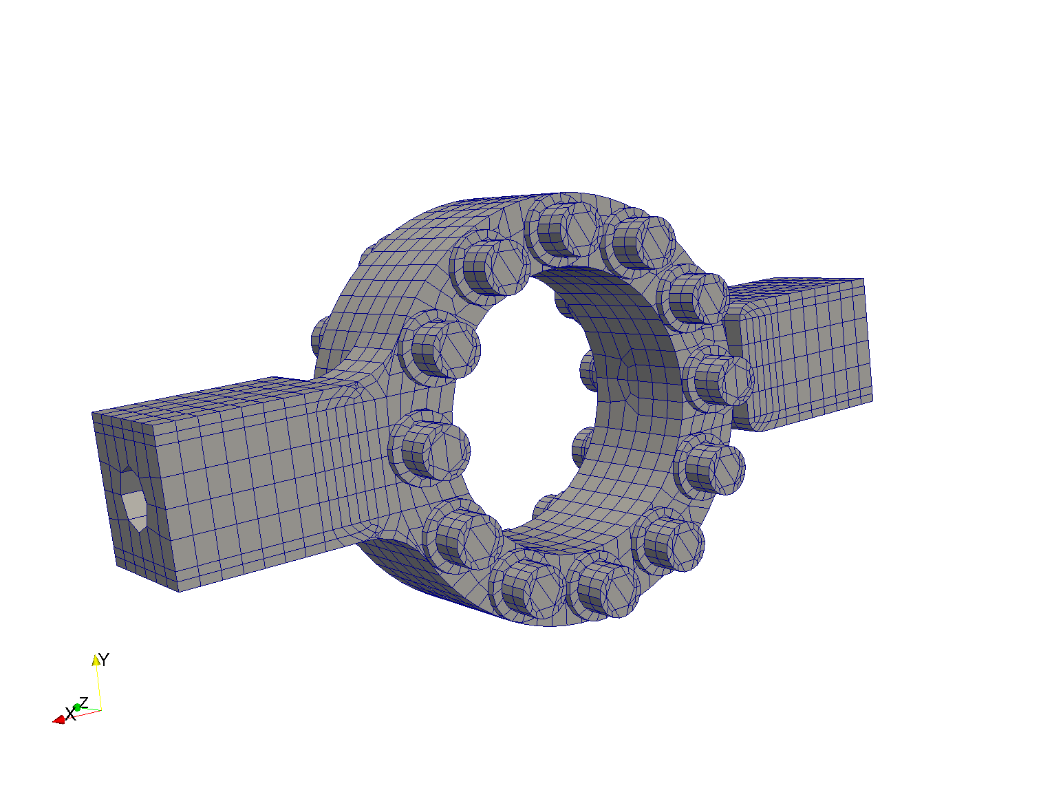
Refer to caption
(a) Finite-element mesh
Refer to caption
(b) Pressure-loaded surface (red), contact surfaces (blue), prescribed temperature (green), Dirichlet boundary condition (gray).
Fig. 1: Pancake problem.

The x𝑥x-, y𝑦y-, and z𝑧z-displacements of the rightmost surface (gray in Figure 1(b)) are set to zero. The x𝑥x- and y𝑦y- displacements of the leftmost surface (red in Figure 1(b)) are set to zero; this surface is also subjected to the time-dependent pressure load depicted in Figure 2(a).
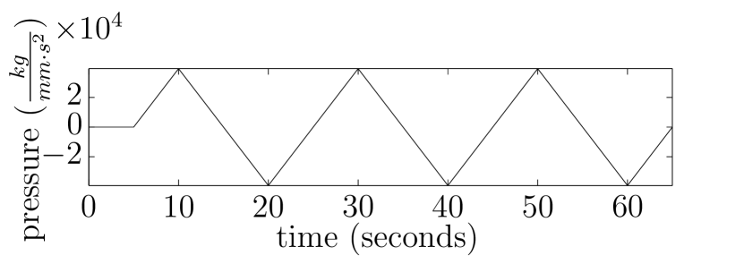
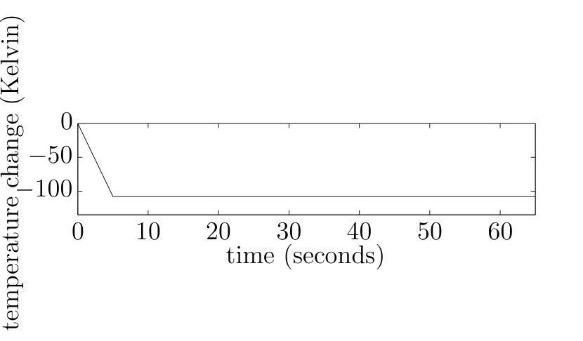
Refer to caption
(a) Time-dependent pressure load applied to leftmost surface (extrema are ±3.94×10⁴kgmms2plus-or-minus3.94superscript104kgmmsuperscripts2\pm 3.94\times 10^{4}\ \frac{\text{kg}}{\text{mm}\cdot\text{s}^{2}}).
Refer to caption
(b) Time-dependent temperature load applied to bolts.
Fig. 2: Time-dependent loadings for the pancake problem.

The time-dependent thermal load depicted in Figure 2(b) is applied to the bolts (green components in Figure 1(b)) to emulate a pre-loading condition. Contact surfaces are shown in blue in Figure 1(b); they are enforced by an augmented Lagrangian approach with DASH search using a penalty factor of 1.25 and a friction coefficient of 0.5.

The problem is discretized by the finite-element method using a mesh generated by the SIERRA toolkit [11]. The mesh consists of 9108 nodes and 4719 hexahedral elements. At each node, there are three degrees of freedom (the x𝑥x-, y𝑦y-, and z𝑧z-displacements), which leads to 27,3242732427,324 total degrees of freedom for the finite-element model.

As the time scales of the load application are relatively large, we neglect inertial effects and consider solving the quasi-static equations

(63) 𝒇int(𝒖i)+𝒇contact(𝒖i,λl)=𝒇ext(ti),l=1,,L,i=1,,T,formulae-sequencesuperscript𝒇intsubscript𝒖𝑖superscript𝒇contactsubscript𝒖𝑖superscript𝜆𝑙superscript𝒇extsubscript𝑡𝑖formulae-sequence𝑙1𝐿𝑖1𝑇\boldsymbol{f}^{\text{int}}\left(\boldsymbol{u}_{i}\right)+\boldsymbol{f}^{\text{contact}}\left(\boldsymbol{u}_{i},\lambda^{l}\right)=\boldsymbol{f}^{\text{ext}}(t_{i}),\quad l=1,\ldots,L,\quad i=1,\ldots,T,

where T𝑇T denotes the number of time steps, 𝒇int:nn:superscript𝒇intsuperscript𝑛superscript𝑛\boldsymbol{f}^{\text{int}}:\mathbb{R}^{n}\rightarrow\mathbb{R}^{n} is a nonlinear operator representing the internal forces, 𝒇contact:n×+n:superscript𝒇contactsuperscript𝑛superscriptsuperscript𝑛\boldsymbol{f}^{\text{contact}}:\mathbb{R}^{n}\times\mathbb{R}^{+}\rightarrow\mathbb{R}^{n} is nonlinear in its first argument and represents contact forces, 𝒇ext:[0,65]n:superscript𝒇ext065superscript𝑛\boldsymbol{f}^{\text{ext}}:\left[0,65\right]\rightarrow\mathbb{R}^{n} is the external-force vector, and 𝒖insubscript𝒖𝑖superscript𝑛\boldsymbol{u}_{i}\in\mathbb{R}^{n} denotes the displacement at time tisubscript𝑡𝑖t_{i}. As the contact constraints are enforced using an augmented Lagrangian approach within a continuation loop, λl+superscript𝜆𝑙superscript\lambda^{l}\in\mathbb{R}^{+} with λlλl+1superscript𝜆𝑙superscript𝜆𝑙1\lambda^{l}\leq\lambda^{l+1}, lNatureL𝑙Nature𝐿l\in{\rm Nature}{L} denotes the penalty factor at continuation iteration l𝑙l. Note that these equations also include equality constraints arising from the Dirichlet boundary conditions.

Solving Eqs. (63) is mathematically equivalent to solving

(64) minimize𝐳ngil(𝐳)𝐳superscript𝑛minimizesuperscriptsubscript𝑔𝑖𝑙𝐳\underset{{\mathbf{z}}\in\mathbb{R}^{n}}{\text{minimize}}\quad g_{i}^{l}({\mathbf{z}})

with gil:𝐳𝒇ext(ti)𝒇int(𝐳)𝒇contact(𝐳,λl):superscriptsubscript𝑔𝑖𝑙maps-to𝐳superscript𝒇extsubscript𝑡𝑖superscript𝒇int𝐳superscript𝒇contact𝐳superscript𝜆𝑙-\nabla g_{i}^{l}:{{\mathbf{z}}}\mapsto\boldsymbol{f}^{\text{ext}}(t_{i})-\boldsymbol{f}^{\text{int}}\left({\mathbf{z}}\right)-\boldsymbol{f}^{\text{contact}}\left({\mathbf{z}},\lambda^{l}\right) for a local minimum. Sierra/SolidMechanics solves problem (64) using the nonlinear conjugate gradient method with a displacement-dependent preconditioner 𝐌¯l:¯𝒖𝒖𝒇int(¯𝒖)+𝒖𝒇contact(¯𝒖,λl)SPD(n):superscript¯𝐌𝑙maps-to¯absent𝒖subscript𝒖superscript𝒇int¯absent𝒖subscript𝒖superscript𝒇contact¯absent𝒖superscript𝜆𝑙SPD𝑛\bar{\mathbf{M}}^{l}:\bar{}\boldsymbol{u}\mapsto\nabla_{\boldsymbol{u}}\boldsymbol{f}^{\text{int}}\left(\bar{}\boldsymbol{u}\right)+\nabla_{\boldsymbol{u}}\boldsymbol{f}^{\text{contact}}\left(\bar{}\boldsymbol{u},\lambda^{l}\right)\in\text{SPD}(n). This results in a sequence of linear systems of the original form in Eqs. (1): one at each nonlinear conjugate-gradient iteration. Here, 𝐀j=𝐌¯l(𝒖il(k))subscript𝐀𝑗superscript¯𝐌𝑙superscriptsubscript𝒖𝑖𝑙𝑘{\mathbf{A}}_{j}=\bar{\mathbf{M}}^{l}(\boldsymbol{u}_{i}^{l(k)}), 𝐛j=gil(𝒖il(k))subscript𝐛𝑗superscriptsubscript𝑔𝑖𝑙superscriptsubscript𝒖𝑖𝑙𝑘{\mathbf{b}}_{j}=\nabla g_{i}^{l}(\boldsymbol{u}_{i}^{l(k)}), 𝒖il(k)nsuperscriptsubscript𝒖𝑖𝑙𝑘superscript𝑛\boldsymbol{u}_{i}^{l(k)}\in\mathbb{R}^{n} denotes the displacement at time step i𝑖i, continuation iteration l𝑙l, and nonlinear conjugate gradient iteration k𝑘k. The mapping between timestep i𝑖i, continuation iteration l𝑙l, nonlinear conjugate-gradient iteration k𝑘k and the index of the linear system j𝑗j is provided by j:(i,l,k)k+𝗂=1i𝗅=1lK(𝗂,𝗅):𝑗maps-to𝑖𝑙𝑘𝑘superscriptsubscript𝗂1𝑖superscriptsubscript𝗅1𝑙𝐾𝗂𝗅j:(i,l,k)\mapsto k+\sum_{\mathsf{i}=1}^{i}\sum_{\mathsf{l}=1}^{l}K(\mathsf{i},\mathsf{l}), where K(i,l)𝐾𝑖𝑙K(i,l) denotes the number of conjugate-gradient iterations needed to solve problem (64).

For this problem, the total number of linear systems we consider is p=47𝑝47p=47. Each of these linear systems is preconditioned using a three-level algebraic multigrid (AMG) preconditioner 𝐌jsubscript𝐌𝑗{\mathbf{M}}_{j} with incomplete Cholesky smoothing for both pre-smoothing and post-smoothing. This preconditioner tends to be expensive to apply, especially when compared with the cost of a matrix–vector product for this system.

5.1.2 Problem 2: I-beam problem
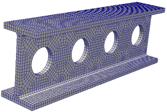
Refer to caption
(a) Finite-element mesh
Refer to caption
(b) Mesh with boundary-condition information.
Fig. 3: I-beam problem.

We next consider computing the quasistatic response (neglecting thermal effects) of an I-beam with holes in the web section; the domain is pictured in Figure 3(a). The material is steel 304L, which is characterized by a Young’s modulus of E=2.1×10⁸Nmms2𝐸2.1superscript108Nmmsuperscripts2E=2.1\times 10^{8}\ \frac{\text{N}}{\text{mm}\ \cdot\ \text{s}^{2}}, Poisson’s ratio of ν=0.33𝜈0.33\nu=0.33, and density of ρ=7.8×10⁶kg/mm3𝜌7.8superscript106kgsuperscriptmm3\rho=7.8\times 10^{-6}\ \text{kg}/\text{mm}^{3}. The x𝑥x-, y𝑦y-, and z𝑧z-displacement of the bottom-left point (blue point in Figure 3(b)) are set to zero. The x𝑥x- and y𝑦y- displacement of the bottom-right point (yellow point in Figure 3(b)) are set to zero. The x𝑥x-displacement of the top-left point (magenta point in Figure 3(b)) is set to zero. Finally, a torsional traction is applied the end surfaces (red and green in Figure 3); Ref. [1, Eq. (11)] reports details on the tractional loading, where the scale factor for the current problem is 0.01. The mesh consists of 13,137 nodes and 8,576 hexahedral elements. Each node is characterized by three degrees of freedom (the x𝑥x-, y𝑦y-, and z𝑧z-displacements), which leads to 39,4113941139,411 total degrees of freedom in the finite-element model.

We again neglect inertial effects and consider solving the quasi-static equations

(65) 𝒇int(𝒖i)=𝒇ext(ti),i=1,,T.formulae-sequencesuperscript𝒇intsubscript𝒖𝑖superscript𝒇extsubscript𝑡𝑖𝑖1𝑇\boldsymbol{f}^{\text{int}}\left(\boldsymbol{u}_{i}\right)=\boldsymbol{f}^{\text{ext}}(t_{i}),\quad i=1,\ldots,T.

These equations also include equality constraints arising from the Dirichlet boundary conditions; note that the continuation loop for computing contact forces does not appear in this problem. Solving Eqs. (65) is equivalent to solving

(66) minimize𝐳ngi(𝐳)𝐳superscript𝑛minimizesubscript𝑔𝑖𝐳\underset{{\mathbf{z}}\in\mathbb{R}^{n}}{\text{minimize}}\quad g_{i}({\mathbf{z}})

with gi:𝐳𝒇ext(ti)𝒇int(𝐳):subscript𝑔𝑖maps-to𝐳superscript𝒇extsubscript𝑡𝑖superscript𝒇int𝐳-\nabla g_{i}:{\mathbf{z}}\mapsto\boldsymbol{f}^{\text{ext}}(t_{i})-\boldsymbol{f}^{\text{int}}\left({\mathbf{z}}\right). We again use the nonlinear conjugate gradient method to solve problem (66); we also again employ a displacement-dependent preconditioner 𝐌¯:𝒖𝒖𝒇int(𝒖)+𝒖𝒇contact(𝒖,λl)SPD(n):¯𝐌maps-to𝒖subscript𝒖superscript𝒇int𝒖subscript𝒖superscript𝒇contact𝒖superscript𝜆𝑙SPD𝑛\bar{\mathbf{M}}:\boldsymbol{u}\mapsto\nabla_{\boldsymbol{u}}\boldsymbol{f}^{\text{int}}\left(\boldsymbol{u}\right)+\nabla_{\boldsymbol{u}}\boldsymbol{f}^{\text{contact}}\left(\boldsymbol{u},\lambda^{l}\right)\in\text{SPD}(n). This results in a sequence of linear systems of the original form in Eqs. (1): one at each nonlinear conjugate-gradient iteration. Here, 𝐀j=𝐌¯(𝒖i(k))subscript𝐀𝑗¯𝐌superscriptsubscript𝒖𝑖𝑘{\mathbf{A}}_{j}=\bar{\mathbf{M}}(\boldsymbol{u}_{i}^{(k)}) and 𝐛j=gi(𝒖i(k))subscript𝐛𝑗subscript𝑔𝑖superscriptsubscript𝒖𝑖𝑘{\mathbf{b}}_{j}=\nabla g_{i}(\boldsymbol{u}_{i}^{(k)}), where the mapping between time step and nonlinear conjugate-gradient iteration is provided by j:(i,k)k+𝗂=1iK(𝗂):𝑗maps-to𝑖𝑘𝑘superscriptsubscript𝗂1𝑖𝐾𝗂j:(i,k)\mapsto k+\sum_{\mathsf{i}=1}^{i}K(\mathsf{i}). Here, K(i)𝐾𝑖K(i) denotes the number of conjugate-gradient iterations needed to solve problem (66). For this problem, the total number of linear systems we consider is p=49𝑝49p=49. Each of these linear systems is preconditioned using the same multigrid preconditioner 𝐌jsubscript𝐌𝑗{\mathbf{M}}_{j} as described in Section 5.1.1; the only modification is that four levels of multigrid are used in this case due to the larger number of degrees of freedom.

5.2 Experimental setup

We implemented our proposed method in Matlab and ran experiments on a Macbook Pro with Intel 2.7 GHz i5 processor and 8 GB of RAM; the implementation performs the linear-system solves after reading in the linear systems generated by Sierra/SolidMechanics as described in Section 5.1.

For all problems, we test our framework using a full-orthogonalization method (FOM) rather than the conjugate-gradient recurrence; this amounts to replacing Step 14 in Algorithm 1 with the following [37]:

  𝐩(k+1)=𝐳(k+1)𝐘𝝁(k+1)superscript𝐩𝑘1superscript𝐳𝑘1𝐘superscript𝝁𝑘1{\mathbf{p}}^{(k+1)}={\mathbf{z}}^{(k+1)}-\mathbf{Y}{\boldsymbol{\mu}}^{(k+1)}
  for i=1,,k𝑖1𝑘i=1,\ldots,k do
        β(k+1),i=(𝐫(k+1))T𝐳(k+1)(𝐫(i))T𝐳(i)superscript𝛽𝑘1𝑖superscriptsuperscript𝐫𝑘1𝑇superscript𝐳𝑘1superscriptsuperscript𝐫𝑖𝑇superscript𝐳𝑖\beta^{(k+1),i}=\frac{({\mathbf{r}}^{(k+1)})^{T}{\mathbf{z}}^{(k+1)}}{({\mathbf{r}}^{(i)})^{T}{\mathbf{z}}^{(i)}}   𝐩(k+1)=𝐩(k+1)+β(k+1),i𝐩(i)superscript𝐩𝑘1superscript𝐩𝑘1superscript𝛽𝑘1𝑖superscript𝐩𝑖{\mathbf{p}}^{(k+1)}={\mathbf{p}}^{(k+1)}+\beta^{(k+1),i}{\mathbf{p}}^{(i)}
  end for

In exact arithmetic, this modification does not affect the solution. However, in finite precision, this modification ensures that that the basis 𝐕jsubscript𝐕𝑗{\mathbf{V}}_{j} is full rank; this is sometimes necessary to ensure nonsingular systems during stage-1 solves. Removing the effect of possible rank deficiency from the numerical experiments also simplifies interpretation of the results.

Iterative-solver performance can be measured in three primary ways: the number of incurred matrix–vector products, the number of stage-3 iterations (which is equal to the number of preconditioner applications), and the wall time per linear-system solve. While the wall time is the most important metric in practice, we report all three metrics (in terms of their averages over all linear systems) to provide a more complete picture of performance, as the specific linear system and choice of preconditioner can have a strong effect on the relative cost of operations.

5.3 Method comparison: Pancake problem

This section compares the following methods:

  1. 1.

    FOM. This approach solves each linear system independently without recycling using the full orthogonalization method.

  2. 2.

    No truncation. This approach does not perform truncation, and employs y¯=¯𝑦\bar{y}=\infty, ϱ=1italic-ϱ1\varrho=1, and φ=0𝜑0\varphi=0 in Algorithm 3. Because it employs all Krylov vectors as the augmenting-subspace basis, it requires the fewest stage-3 iterations and, thus, the fewest number of preconditioner applications; however, the memory and orthogonalization costs are the largest for this method.

  3. 3.

    DF(100,0). This is the standard approach for deflation-based truncation, which places all augmenting-subspace basis vectors in the stage-1 basis. Here, Algorithm 3 parameters are y¯=200¯𝑦200\bar{y}=200, ϱ=1italic-ϱ1\varrho=1, φ=0𝜑0\varphi=0, and 𝐖j+1=[[𝐘j+1]1[𝐘j+1]100]subscript𝐖𝑗1delimited-[]subscriptdelimited-[]subscript𝐘𝑗11subscriptdelimited-[]subscript𝐘𝑗1100\mathbf{W}_{j+1}=\left[\left[\mathbf{Y}_{j+1}\right]_{1}\ \cdots\ \left[\mathbf{Y}_{j+1}\right]_{100}\right] in step 27. In step 25, the augmenting space is computed by solving Eq. (25) for jj+1𝑗𝑗1j\leftarrow j+1 and setting 𝐘j+1[𝐙j+1𝐠1𝐙j+1𝐠100]subscript𝐘𝑗1delimited-[]subscript𝐙𝑗1subscript𝐠1subscript𝐙𝑗1subscript𝐠100\mathbf{Y}_{j+1}\leftarrow\left[\mathbf{Z}_{j+1}\mathbf{g}_{1}\ \cdots\ \mathbf{Z}_{j+1}\mathbf{g}_{100}\right].

  4. 4.

    POD(100,0). This approach employs POD truncation and places augmenting-subspace basis vectors in the stage-1 basis. Algorithm 3 parameters are y¯=200¯𝑦200\bar{y}=200, ϱ=1italic-ϱ1\varrho=1, φ=0𝜑0\varphi=0, 𝐘j+1=𝐔100𝐀j(𝐙j+1,𝜼jRBF(jj¯))subscript𝐘𝑗1subscriptsuperscript𝐔subscript𝐀𝑗100subscript𝐙𝑗1subscriptsuperscript𝜼RBF𝑗𝑗¯𝑗\mathbf{Y}_{j+1}={\mathbf{U}}^{{\mathbf{A}}_{j}}_{100}\left(\mathbf{Z}_{j+1},\boldsymbol{\eta}^{\text{RBF}}_{j}(j-\bar{j})\right) in step 25, and 𝐖j+1=[[𝐘j+1]1[𝐘j+1]100]subscript𝐖𝑗1delimited-[]subscriptdelimited-[]subscript𝐘𝑗11subscriptdelimited-[]subscript𝐘𝑗1100\mathbf{W}_{j+1}=\left[\left[\mathbf{Y}_{j+1}\right]_{1}\ \cdots\ \left[\mathbf{Y}_{j+1}\right]_{100}\right] in step 27.

  5. 5.

    POD(5,95)it stg1. This approach employs POD truncation, places only the dominant POD modes in the stage-1 basis, and places all post-truncation Krylov vectors in the stage-1 basis. Algorithm 3 parameters are y¯=200¯𝑦200\bar{y}=200, ϱ=1italic-ϱ1\varrho=1, φ=1𝜑1\varphi=1, 𝐘j+1=𝐔100𝐀j(𝐙j+1,𝜼jRBF(jj¯))subscript𝐘𝑗1subscriptsuperscript𝐔subscript𝐀𝑗100subscript𝐙𝑗1subscriptsuperscript𝜼RBF𝑗𝑗¯𝑗\mathbf{Y}_{j+1}={\mathbf{U}}^{{\mathbf{A}}_{j}}_{100}\left(\mathbf{Z}_{j+1},\boldsymbol{\eta}^{\text{RBF}}_{j}(j-\bar{j})\right) in step 25, and 𝐖j+1=[[𝐘j+1]1[𝐘j+1]5]subscript𝐖𝑗1delimited-[]subscriptdelimited-[]subscript𝐘𝑗11subscriptdelimited-[]subscript𝐘𝑗15\mathbf{W}_{j+1}=\left[\left[\mathbf{Y}_{j+1}\right]_{1}\ \cdots\ \left[\mathbf{Y}_{j+1}\right]_{5}\right] in step 27. Note that ϵ^j=104ϵjsubscript^italic-ϵ𝑗superscript104subscriptitalic-ϵ𝑗\hat{\epsilon}_{j}=10^{-4}\epsilon_{j} for ϵj103subscriptitalic-ϵ𝑗superscript103\epsilon_{j}\geq 10^{-3}, and ϵ^j=105ϵjsubscript^italic-ϵ𝑗superscript105subscriptitalic-ϵ𝑗\hat{\epsilon}_{j}=10^{-5}\epsilon_{j} otherwise, while ϵ¯j=102ϵjsubscript¯italic-ϵ𝑗superscript102subscriptitalic-ϵ𝑗\bar{\epsilon}_{j}=10^{-2}\epsilon_{j} for all tolerances.

  6. 6.

    POD(5,95)it mixed. This approach employs POD truncation, places only the dominant POD modes in the stage-1 basis, and places only the dominant post-truncation Krylov vectors in the stage-1 basis. Algorithm 3 parameters are employs y¯=200¯𝑦200\bar{y}=200, ϱ=1×10³italic-ϱ1superscript103\varrho=1\times 10^{-3}, φ=1𝜑1\varphi=1, 𝐘j+1=𝐔100𝐀j(𝐙j+1,𝜼jRBF(jj¯))subscript𝐘𝑗1subscriptsuperscript𝐔subscript𝐀𝑗100subscript𝐙𝑗1subscriptsuperscript𝜼RBF𝑗𝑗¯𝑗\mathbf{Y}_{j+1}={\mathbf{U}}^{{\mathbf{A}}_{j}}_{100}\left(\mathbf{Z}_{j+1},\boldsymbol{\eta}^{\text{RBF}}_{j}(j-\bar{j})\right) in step 25, and 𝐖j+1=[[𝐘j+1]1[𝐘j+1]5]subscript𝐖𝑗1delimited-[]subscriptdelimited-[]subscript𝐘𝑗11subscriptdelimited-[]subscript𝐘𝑗15\mathbf{W}_{j+1}=\left[\left[\mathbf{Y}_{j+1}\right]_{1}\ \cdots\ \left[\mathbf{Y}_{j+1}\right]_{5}\right] in step 27. Note ϵ^j=104ϵjsubscript^italic-ϵ𝑗superscript104subscriptitalic-ϵ𝑗\hat{\epsilon}_{j}=10^{-4}\epsilon_{j} for ϵj102subscriptitalic-ϵ𝑗superscript102\epsilon_{j}\geq 10^{-2}, and ϵ^j=106ϵjsubscript^italic-ϵ𝑗superscript106subscriptitalic-ϵ𝑗\hat{\epsilon}_{j}=10^{-6}\epsilon_{j} otherwise and ϵ¯j=102ϵjsubscript¯italic-ϵ𝑗superscript102subscriptitalic-ϵ𝑗\bar{\epsilon}_{j}=10^{-2}\epsilon_{j} for all ϵjsubscriptitalic-ϵ𝑗\epsilon_{j}.

  7. 7.

    POD(5,95)it stg2. This approach employs POD truncation, places only the dominant POD modes in the stage-1 basis, and places none of the post-truncation Krylov vectors in the stage-1 basis. Algorithm 3 parameters are employs y¯=200¯𝑦200\bar{y}=200, ϱ=0italic-ϱ0\varrho=0, φ=1𝜑1\varphi=1, 𝐘j+1=𝐔100𝐀j(𝐙j+1,𝜼jRBF(jj¯))subscript𝐘𝑗1subscriptsuperscript𝐔subscript𝐀𝑗100subscript𝐙𝑗1subscriptsuperscript𝜼RBF𝑗𝑗¯𝑗\mathbf{Y}_{j+1}={\mathbf{U}}^{{\mathbf{A}}_{j}}_{100}\left(\mathbf{Z}_{j+1},\boldsymbol{\eta}^{\text{RBF}}_{j}(j-\bar{j})\right) in step 25, and 𝐖j+1=[[𝐘j+1]1[𝐘j+1]5]subscript𝐖𝑗1delimited-[]subscriptdelimited-[]subscript𝐘𝑗11subscriptdelimited-[]subscript𝐘𝑗15\mathbf{W}_{j+1}=\left[\left[\mathbf{Y}_{j+1}\right]_{1}\ \cdots\ \left[\mathbf{Y}_{j+1}\right]_{5}\right] in step 27. Note ϵ^j=104ϵjsubscript^italic-ϵ𝑗superscript104subscriptitalic-ϵ𝑗\hat{\epsilon}_{j}=10^{-4}\epsilon_{j} for ϵj102subscriptitalic-ϵ𝑗superscript102\epsilon_{j}\geq 10^{-2}, and ϵ^j=107ϵjsubscript^italic-ϵ𝑗superscript107subscriptitalic-ϵ𝑗\hat{\epsilon}_{j}=10^{-7}\epsilon_{j} otherwise. ϵ¯j=102ϵjsubscript¯italic-ϵ𝑗superscript102subscriptitalic-ϵ𝑗\bar{\epsilon}_{j}=10^{-2}\epsilon_{j} for ϵj103subscriptitalic-ϵ𝑗superscript103\epsilon_{j}\geq 10^{-3} and ϵ¯j=103ϵjsubscript¯italic-ϵ𝑗superscript103subscriptitalic-ϵ𝑗\bar{\epsilon}_{j}=10^{-3}\epsilon_{j} otherwise.

Refer to caption
(a) All methods
Refer to caption
(b) Recycling methods only
Fig. 4: Pancake problem: average number of matrix–vector products, preconditioner applications, and wall time to compute solutions within tolerances ϵj=101subscriptitalic-ϵ𝑗superscript101\epsilon_{j}=10^{-1} through ϵj=106subscriptitalic-ϵ𝑗superscript106\epsilon_{j}=10^{-6}.

Figure 4(a) reports results for all tested methods. First, we note that applying the AMG preconditioner is computationally expensive for this problem, especially relative to matrix–vector products. Therefore, there is a strong relationship between the wall-time performance and the preconditions-application performance of iterative methods for this example. Next, we note that recycling provides a significant benefit, as applying FOM without recycling is the slowest method for all tested tolerances. To more clearly distinguish the differences between recycling methods, Figure 4(b) reports the same results with the FOM performance removed. Here, we see that the no-truncation case yields the best performance as measured in both wall time and preconditioner applications; however, it performs the worst in matrix–vector products. This arises from two primary effects: 1) the preconditioner application is the dominant cost for this problem, so minimizing the number of stage-3 iterations—which will always occur by not truncating the augmenting subspace—yields the best wall time performance, and 2) the problem is small scale, so there is not a significant penalty to retaining all Krylov vectors. We also note that the POD methods (especially the POD(100,0) method) perform similarly to the no truncation method; this suggests that POD truncation effectively captures the most important subspace from the set of available vectors.

Next, we note that the ‘inner’ iterative method described in Section 4.3.1—which is used by the three POD(5,95) methods—produces the same number of preconditioner applications as POD(100,0). This illustrates that the inner iterative method has successfully orthogonalized against the entire augmenting subspace. Figure 5 illustrates this point further by comparing three methods: the POD(5,95)it stg1 method, the POD(5,95) stg1 method (which is identical to POD(5,95)it stg1 except that it employs φ=0𝜑0\varphi=0 in Algorithm 3), and the POD(100,0) method. While POD(5,95)it stg1 matches the preconditioning applications of POD(100,0), this comes at the cost of additional matrix–vector products for stricter tolerances; further these matrix–vector products are generally not applied as a block as in POD(100,0), which makes them more expensive on average. In addition, the cost of repeatedly multiplying vectors by the full augmenting-subspace basis 𝐘jsubscript𝐘𝑗\mathbf{Y}_{j} within the inner iterative method is not counted toward matrix–vector products, even though this operation incurs a non-negligible cost due to the density of 𝐘jsubscript𝐘𝑗\mathbf{Y}_{j}. As a result, POD(100,0) yields the lowest wall time; we might expect POD(5,95)it stg1 to produce a lower wall time when the dimension of the augmenting subspace is larger.
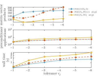
Refer to caption
Fig. 5: Comparison of iterative and non-iterative Stage 3 for the problem 1.

As was shown in Theorem 6, the reduced matrix 𝐘jT𝐀j𝐘jsuperscriptsubscript𝐘𝑗𝑇subscript𝐀𝑗subscript𝐘𝑗\mathbf{Y}_{j}^{T}{\mathbf{A}}_{j}\mathbf{Y}_{j} should be well conditioned if the system matrices do not vary significantly. Figure 6 illustrates this effect: the condition number of the reduced system is close to one for all linear systems. This implies fast convergence of stage 2. Note that this effect comes ‘for free’ when employing a POD metric of 𝐀j¯subscript𝐀¯𝑗{\mathbf{A}}_{\bar{j}}, as the basis is automatically 𝐀j¯subscript𝐀¯𝑗{\mathbf{A}}_{\bar{j}}-orthogonal; this precludes the need for orthogonalization step 26 in Algorithm 3 as was noted in Section 4.4.1.
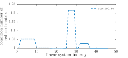
Refer to caption
Fig. 6: Condition number for reduced linear systems.

5.4 Method comparison: I-beam problem

We compare the same methods as in Section 5.3; the only modification is that all POD(5,95) methods employ parameters ϵ^j=104ϵjsubscript^italic-ϵ𝑗superscript104subscriptitalic-ϵ𝑗\hat{\epsilon}_{j}=10^{-4}\epsilon_{j}, ϵ¯j=102ϵjsubscript¯italic-ϵ𝑗superscript102subscriptitalic-ϵ𝑗\bar{\epsilon}_{j}=10^{-2}\epsilon_{j} in Algorithm 3.

Figure 7(a) reports results for all tested methods. Again, we first note that the use of recycling leads to significant improvements, as the FOM method (without recycling) produces the largest wall time and requires the largest number of preconditioner applications. To more easily distinguish the relative merits of the recycling methods, Figure 7(b) reports the results without FOM. This figure illustrates the need for truncation within recycling. As for the pancake problem, the ‘no truncation’ case minimizes the number of preconditioner applications; however, the lower matrix–vector multiplication cost and the lower overhead in the stage-3 orthogonalization steps lead to lower overall costs for several truncation methods. Figure 7(b) also illustrates the benefit of using the hybrid direct/iterative approach to solve over the augmenting subspace, as POD(5,95)it stg2—which employs this approach—produces the lowest wall time and number of matrix–vector products for all tested tolerances. We also note that all POD-based truncation methods outperform deflation in terms of preconditioner applications; all POD methods except for POD(5,95)it mixed also outperform deflation in terms of matrix–vector multiplications and wall time.
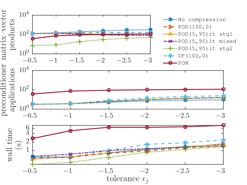
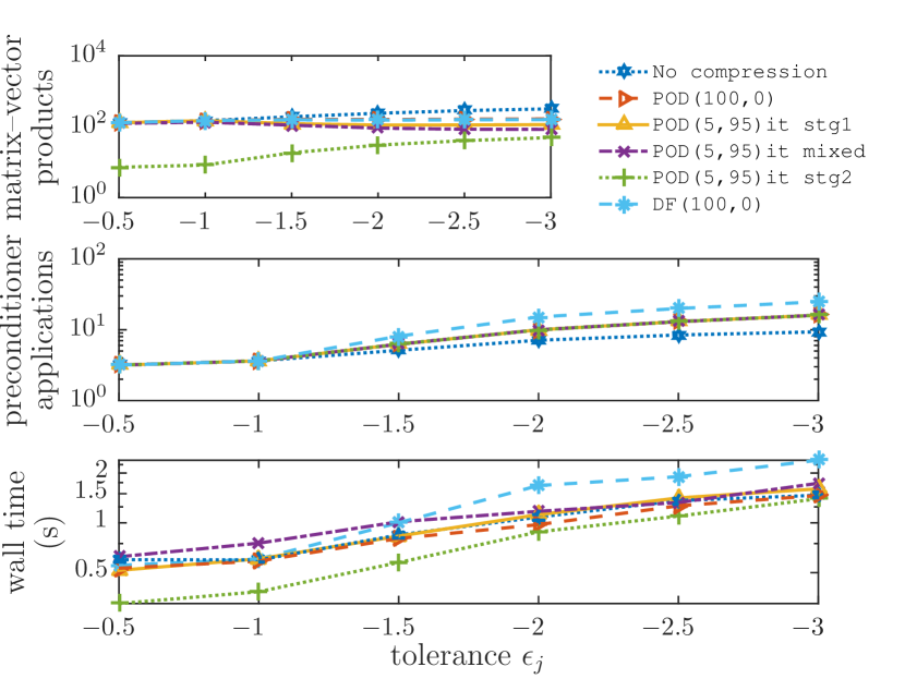
Refer to caption
(a) All methods
Refer to caption
(b) Recycling methods only
Fig. 7: I-beam problem: average number of matrix–vector products, preconditioner applications, and wall time to compute solutions within tolerances ϵj=100.5subscriptitalic-ϵ𝑗superscript100.5\epsilon_{j}=10^{-0.5} through ϵj=103subscriptitalic-ϵ𝑗superscript103\epsilon_{j}=10^{-3}.

Finally, Figure 8 assess the performance of the ‘inner’ iterative method proposed in Section 4.3.1, which aims to orthogonalize against the entire augmenting subspace within stage 3 using an iterative method. These data show that the iterative method in POD(5,95)it stg1 successfully matches the number of stage-3 iterations (i.e., preconditioner applications) as POD(100,0), yet it incurs far fewer matrix–vector products. In fact, the number of matrix–vector products is close to that realized by POD(5,95) stg1 without the inner iterative method.
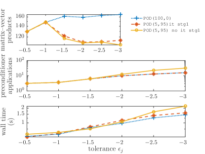
Refer to caption
Fig. 8: I-beam problem: POD-method performance in terms of average number of matrix–vector products, preconditioner applications, and wall time to compute solutions within tolerances ϵj=100.5subscriptitalic-ϵ𝑗superscript100.5\epsilon_{j}=10^{-0.5} through ϵj=103subscriptitalic-ϵ𝑗superscript103\epsilon_{j}=10^{-3}.

5.5 POD-weights experiments

This section compares the performance of POD-based truncation methods when various POD weights are employed (see Section 3.3.2). To assess this, POD truncation is performed after the solution of the first ten linear systems, and performance of the resulting truncated augmented subspace is assessed for the eleventh linear system. That is, we propose computing the truncated augmenting subspace according to

(67) 𝒴11=𝒰y11𝐀10(𝐙10,𝜸)subscript𝒴11subscriptsuperscript𝒰subscript𝐀10subscript𝑦11subscript𝐙10𝜸\mathcal{Y}_{11}=\mathcal{U}^{{\mathbf{A}}_{10}}_{y_{11}}\left(\mathbf{Z}_{10},\boldsymbol{\gamma}\right)

for various choices of 𝜸𝜸\boldsymbol{\gamma}. We compare the following POD weights proposed in Section 3.3.2:

  1. 1.

    Ideal weights. This case employs 𝜸=𝜼11𝜸subscriptsuperscript𝜼11\boldsymbol{\gamma}=\boldsymbol{\eta}^{\star}_{11} as defined in Eq. (34). Although this weighting scheme is not practical, it illustrates the best possible choice.

  2. 2.

    Previous weights. This case employs 𝜸=𝜼11prev𝜸subscriptsuperscript𝜼prev11\boldsymbol{\gamma}=\boldsymbol{\eta}^{\text{prev}}_{11} as defined in Eq. (36).

  3. 3.

    Radial-basis-function weights. This case employs 𝜸=𝜼11RBF(11)𝜸subscriptsuperscript𝜼RBF1111\boldsymbol{\gamma}=\boldsymbol{\eta}^{\text{RBF}}_{11}(11) as defined in Eq. (40). This is the choice used by the previous experiments in this section.
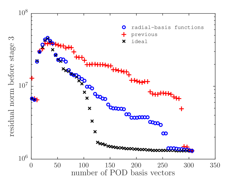
Refer to caption
(a) The residual norm before stage 3 as a function of the number of POD vectors k𝑘k.
Refer to caption
(b) Number of stage-3 iterations taken to satisfy a tolerance of ϵ11=106subscriptitalic-ϵ11superscript106\epsilon_{11}=10^{-6} as a function of the number of POD vectors k𝑘k.
Fig. 9: Pancake problem: POD-weights experiments. Results correspond to solving linear system eleven after performing POD-based truncation for linear system ten using radial-basis-function weights, previous weights, and ideal weights.

Figure 9(a) illustrates that the ideal weights minimize the residual after the reduced system is solved, which implies that the ideal weights lead to a better estimate of the solution in the augmenting subspace. Note that the radial-basis-function weights (which was employed for POD results in previous sections) yields results that are close to the ideal case. Figure 9(b) shows that the ideal weights also minimize the number of stage-3 iterations, while the two other methods produce a similar number of stage-3 iterations as the ideal-weights case. This suggests that radial-basis-function weights provide a good approximation of the ideal weights for both producing an accurate solution in the augmenting subspace and yielding similar stage-3 convergence.

5.6 Output-oriented POD experiments

This section assesses the performance of output-oriented POD, i.e., when the metric is set to 𝚯=𝐂T𝐂𝚯superscript𝐂𝑇𝐂{\boldsymbol{\Theta}}={\mathbf{C}}^{T}{\mathbf{C}} as proposed in Section 3.3.3. For this purpose, we consider a set of q=100𝑞100q=100 output quantities of interest that are random linear functionals of the solution; as such 𝐂[0,1]100×n𝐂superscript01100𝑛{\mathbf{C}}\in[0,1]^{100\times n} with entries drawn from a uniform distribution in the interval [0,1]01[0,1]. In addition to assessing the performance of the No truncation, DF(100,0), and POD(100,0) as described in Section 5.4, we also compare the following methods:

  1. 1.

    POD(5,95). This approach employs POD truncation, places only the dominant POD modes in the stage-1 basis, and places all post-truncation Krylov vectors in the stage-1 basis. Algorithm 3 parameters are y¯=200¯𝑦200\bar{y}=200, ϱ=1italic-ϱ1\varrho=1, φ=0𝜑0\varphi=0, 𝐘j+1=𝐔100𝐀j(𝐙j+1,𝜼jRBF(jj¯))subscript𝐘𝑗1subscriptsuperscript𝐔subscript𝐀𝑗100subscript𝐙𝑗1subscriptsuperscript𝜼RBF𝑗𝑗¯𝑗\mathbf{Y}_{j+1}={\mathbf{U}}^{{\mathbf{A}}_{j}}_{100}\left(\mathbf{Z}_{j+1},\boldsymbol{\eta}^{\text{RBF}}_{j}(j-\bar{j})\right) in step 25, and 𝐖j+1=[[𝐘j+1]1[𝐘j+1]5]subscript𝐖𝑗1delimited-[]subscriptdelimited-[]subscript𝐘𝑗11subscriptdelimited-[]subscript𝐘𝑗15\mathbf{W}_{j+1}=\left[\left[\mathbf{Y}_{j+1}\right]_{1}\ \cdots\ \left[\mathbf{Y}_{j+1}\right]_{5}\right] in step 27.

  2. 2.

    POD(5,95)it. This approach employs POD truncation, places only the dominant POD modes in the stage-1 basis, and places all post-truncation Krylov vectors in the stage-1 basis. Algorithm 3 parameters are y¯=200¯𝑦200\bar{y}=200, ϱ=1italic-ϱ1\varrho=1, φ=1𝜑1\varphi=1, 𝐘j+1=𝐔100𝐀j(𝐙j+1,𝜼jRBF(jj¯))subscript𝐘𝑗1subscriptsuperscript𝐔subscript𝐀𝑗100subscript𝐙𝑗1subscriptsuperscript𝜼RBF𝑗𝑗¯𝑗\mathbf{Y}_{j+1}={\mathbf{U}}^{{\mathbf{A}}_{j}}_{100}\left(\mathbf{Z}_{j+1},\boldsymbol{\eta}^{\text{RBF}}_{j}(j-\bar{j})\right) in step 25, and 𝐖j+1=[[𝐘j+1]1[𝐘j+1]5]subscript𝐖𝑗1delimited-[]subscriptdelimited-[]subscript𝐘𝑗11subscriptdelimited-[]subscript𝐘𝑗15\mathbf{W}_{j+1}=\left[\left[\mathbf{Y}_{j+1}\right]_{1}\ \cdots\ \left[\mathbf{Y}_{j+1}\right]_{5}\right] in step 27. Note that ϵ¯j=102ϵjsubscript¯italic-ϵ𝑗superscript102subscriptitalic-ϵ𝑗\bar{\epsilon}_{j}=10^{-2}\epsilon_{j}.

  3. 3.

    POD-CTCsuperscript𝐶𝑇𝐶C^{T}C(100,0). Identical to POD(100,0) except for 𝐘j+1=𝐔100𝐂T𝐂(𝐙j+1,𝜼jRBF(jj¯))subscript𝐘𝑗1subscriptsuperscript𝐔superscript𝐂𝑇𝐂100subscript𝐙𝑗1subscriptsuperscript𝜼RBF𝑗𝑗¯𝑗\mathbf{Y}_{j+1}={\mathbf{U}}^{{\mathbf{C}}^{T}{\mathbf{C}}}_{100}\left(\mathbf{Z}_{j+1},\boldsymbol{\eta}^{\text{RBF}}_{j}(j-\bar{j})\right).

  4. 4.

    POD-CTCsuperscript𝐶𝑇𝐶C^{T}C(5,95). Identical to POD(5.95) except for 𝐘j+1=𝐔100𝐂T𝐂(𝐙j+1,𝜼jRBF(jj¯))subscript𝐘𝑗1subscriptsuperscript𝐔superscript𝐂𝑇𝐂100subscript𝐙𝑗1subscriptsuperscript𝜼RBF𝑗𝑗¯𝑗\mathbf{Y}_{j+1}={\mathbf{U}}^{{\mathbf{C}}^{T}{\mathbf{C}}}_{100}\left(\mathbf{Z}_{j+1},\boldsymbol{\eta}^{\text{RBF}}_{j}(j-\bar{j})\right).

  5. 5.

    POD-CTCsuperscript𝐶𝑇𝐶C^{T}C(5,95)it. Identical to POD(5.95) except for 𝐘j+1=𝐔100𝐂T𝐂(𝐙j+1,𝜼jRBF(jj¯))subscript𝐘𝑗1subscriptsuperscript𝐔superscript𝐂𝑇𝐂100subscript𝐙𝑗1subscriptsuperscript𝜼RBF𝑗𝑗¯𝑗\mathbf{Y}_{j+1}={\mathbf{U}}^{{\mathbf{C}}^{T}{\mathbf{C}}}_{100}\left(\mathbf{Z}_{j+1},\boldsymbol{\eta}^{\text{RBF}}_{j}(j-\bar{j})\right).

To assess the performance of output-oriented POD truncation—which aims to accurately represent the output quantity of interest—we monitor the error of the solution in the output-oriented norm 𝐱j𝐱j(k)𝐂T𝐂subscriptnormsuperscriptsubscript𝐱𝑗superscriptsubscript𝐱𝑗𝑘superscript𝐂𝑇𝐂||{\mathbf{x}}_{j}^{\star}-{\mathbf{x}}_{j}^{(k)}||_{{\mathbf{C}}^{T}{\mathbf{C}}}. For the pancake problem, we employ ϵj=106subscriptitalic-ϵ𝑗superscript106\epsilon_{j}=10^{-6}, while we use ϵj=103subscriptitalic-ϵ𝑗superscript103\epsilon_{j}=10^{-3} for the I-beam problem. During the execution of the stage-3 algorithm, we track the output-oriented error and report the average number of matrix–vector products, preconditioner applications, and wall time for the error to satisfy 𝐱j𝐱j(k)𝐂T𝐂<τsubscriptnormsuperscriptsubscript𝐱𝑗superscriptsubscript𝐱𝑗𝑘superscript𝐂𝑇𝐂𝜏||{\mathbf{x}}_{j}^{\star}-{\mathbf{x}}_{j}^{(k)}||_{{\mathbf{C}}^{T}{\mathbf{C}}}<\tau for a variety of output-oriented tolerances τ𝜏\tau.

Refer to caption
(a) Pancake problem: stage-1 methods only.
Refer to caption
(b) Pancake problem: stage-1 and stage-2 methods.
Refer to caption
(c) I-beam problem: stage-1 methods only.
Refer to caption
(d) I-beam problem: stage-1 and stage-2 methods.
Fig. 10: Output-oriented truncation experiments: average number of matrix–vector products, preconditioner applications, and wall time to compute solutions as a function of the output-oriented tolerance τ𝜏\tau. Note that (average) preconditioner applications below one indicate that the solution satisfied the specified tolerance before entering stage 3.

Figures 10(a)10(d) compare the performances of the assessed methods as a function of the output-oriented tolerance τ𝜏\tau. First, note that Figures 10(a)10(b) show that POD-based truncation methods produce the lowest wall times for inexact output-oriented tolerances for the pancake problem. These plots also illustrate the benefit of output-oriented metric over the 𝐀jsubscript𝐀𝑗{\mathbf{A}}_{j}-metric: Figure 10(a) shows the superior performance of the former for modest output-oriented tolerances, i.e., those between τ=104𝜏superscript104\tau=10^{-4} and 107superscript10710^{-7}. Figure 10(b) shows that the POD(5,95) methods without the inner iterative method described in Section 4.3.1 are faster for inexact output-oriented tolerances; this occurs because very few stage-3 iterations are required for convergence in the output-oriented norm to these tolerances. In contrast, for stricter tolerances τ106𝜏superscript106\tau\leq 10^{-6}, the inner iterative modification (or no truncation) yields superior performance.

Figures 10(c)10(d) present results for the I-beam problem. These results illustrate the advantage to using the output-oriented metric for most values of the output-oriented tolerance τ𝜏\tau, as POD-CTCsuperscript𝐶𝑇𝐶C^{T}C(100,0) produces the lowest wall time in Figure 10(c) and the POD-CTCsuperscript𝐶𝑇𝐶C^{T}C(5,95)it method produces the lowest wall time for τ103𝜏superscript103\tau\leq 10^{-3}.

Finally, we repeat the POD-weights experiments discussed in Section 5.5 for the output-oriented POD-based truncation method applied to the pancake problem. The experiments measure the number of stage-3 iterations required to converge to a output-oriented tolerance of τ=106𝜏superscript106\tau=10^{-6} as a function of the dimension of the augmenting subspace. We employ a stage-3 tolerance of ϵj=108subscriptitalic-ϵ𝑗superscript108\epsilon_{j}=10^{-8} to accrue the search directions for the first 10 linear systems and subsequently perform truncation using the output-oriented POD metric with different POD weights. The resulting stage-3 iterations are for the eleventh linear system. As we observed for the 𝐀jsubscript𝐀𝑗{\mathbf{A}}_{j}-metric, Figure 11 shows that the ideal weights yield the best performance, as they minimizing the number of stage-3 iterations required for convergence in the output-oriented norm, while the other weighting schemes closely follow the ideal weights.
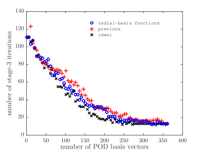
Refer to caption
Fig. 11: Number of stage-3 iterations taken to satisfy an output-oriented tolerance of τ=106𝜏superscript106\tau=10^{-6} for the pancake problem as a function of the augmenting-subspace dimension k𝑘k for radial-basis-function weights, previous weights, and ideal weights.

6 Conclusions

This work has proposed a novel strategy for Krylov-subpace recycling inspired by goal-oriented proper orthogonal decomposition (POD). We performed analyses that expose the close connection between model reduction and Krylov-subspace recycling, proposed specific goal-oriented POD ingredients for truncating previous Krylov vectors, and developed a new ‘three-stage’ algorithm that employs a hybrid direct/iterative approach for efficiently solving over the sum of augmenting and Krylov subspaces. Results on several solid-mechanics problems highlighted the benefits of the new contributions, especially for efficiently computing quantities of interest to modest tolerances.

Acknowledgments

We thank Paul Tsuji for his contributions to obtaining the linear systems used in the numerical experiments, as well as Kendall Pierson for his assistance in using Adagio. We also thank Howard Elman for both insightful conversations and his support in establishing this collaboration. We are also grateful to Eric de Sturler and Michael Parks for fruitful conversations an invaluable suggestions. Sandia National Laboratories is a multi-program laboratory managed and operated by Sandia Corporation, a wholly owned subsidiary of Lockheed Martin Corporation, for the U.S. Department of Energy’s National Nuclear Security Administration under contract DE-AC04-94AL85000. The content of this publication does not necessarily reflect the position or policy of any of these institutions, and no official endorsement should be inferred.

Appendix A POD computation

This section describes two techniques for computing a POD basis using given snapshots, weights, and a pseudometric (see Ref. [4] for additional details). Algorithm 4 describes the first technique, which is based on the eigenvalue decomposition and is equivalent to the well-known “method of snapshots” [41]. Algorithm 5 reports the second case, which is based on the singular value decomposition (SVD) and is more appropriate when the symmetric factorization 𝚯=(𝚯1/2)T𝚯1/2𝚯superscriptsuperscript𝚯12𝑇superscript𝚯12{\boldsymbol{\Theta}}=({\boldsymbol{\Theta}}^{1/2})^{T}{\boldsymbol{\Theta}}^{1/2} is available, where 𝚯1/2superscript𝚯12{\boldsymbol{\Theta}}^{1/2} need not be upper triangular; this approach leads to a more well-conditioned linear system. Note that Algorithms 4 and 5 produce equivalent POD bases (in exact arithmetic) and differ only in their first two steps.

Algorithm 4 pod_evd
0:  snapshot matrix 𝐒n×s𝐒superscript𝑛𝑠{\mathbf{S}}\in\mathbb{R}^{n\times s}, weights 𝜸s𝜸superscript𝑠\boldsymbol{\gamma}\in\mathbb{R}^{s}, pseudometric 𝚯SPSD(n)𝚯SPSD𝑛{\boldsymbol{\Theta}}\in\text{SPSD}(n), and energy criterion ε[0,1]𝜀01\varepsilon\in[0,1]
0:  POD basis 𝐔y𝚯(𝐒,(γ1,,γs))subscriptsuperscript𝐔𝚯𝑦𝐒subscript𝛾1subscript𝛾𝑠{\mathbf{U}}^{{\boldsymbol{\Theta}}}_{y}\left({\mathbf{S}},\left(\gamma_{1},\ldots,\gamma_{s}\right)\right)
1:  𝚯¯=diag(γ1,,γs)𝐒T𝚯𝐒diag(γ1,,γs)¯𝚯diagsubscript𝛾1subscript𝛾𝑠superscript𝐒𝑇𝚯𝐒diagsubscript𝛾1subscript𝛾𝑠\bar{\boldsymbol{\Theta}}=\text{diag}\left(\gamma_{1},\ldots,\gamma_{s}\right){\mathbf{S}}^{T}{\boldsymbol{\Theta}}{\mathbf{S}}\text{diag}\left(\gamma_{1},\ldots,\gamma_{s}\right)
2:   Compute symmetric eigenvalue decomposition 𝚯¯=𝐕𝚺2𝐕T¯𝚯𝐕superscript𝚺2superscript𝐕𝑇\bar{\boldsymbol{\Theta}}=\mathbf{V}\boldsymbol{\Sigma}^{2}\mathbf{V}^{T}
3:  Choose dimension of truncated basis y=miniAi𝑦subscript𝑖𝐴𝑖y=\min_{i\in A}i with A:={iNaturerank(𝚯¯)|k=1iσk2/=1sσ2ε}assign𝐴conditional-set𝑖Naturerank¯𝚯superscriptsubscript𝑘1𝑖superscriptsubscript𝜎𝑘2superscriptsubscript1𝑠superscriptsubscript𝜎2𝜀A\vcentcolon=\{i\in{\rm Nature}{\text{rank}(\bar{\boldsymbol{\Theta}})}\ |\ \sum_{k=1}^{i}\sigma_{k}^{2}/\sum_{\ell=1}^{s}\sigma_{\ell}^{2}\geq\varepsilon\}
4:  𝐔y𝚯(𝐒,𝜸)=𝐒diag(γ1,,γs)[1σ1𝐯11σy𝐯y]subscriptsuperscript𝐔𝚯𝑦𝐒𝜸𝐒diagsubscript𝛾1subscript𝛾𝑠delimited-[]1subscript𝜎1subscript𝐯11subscript𝜎𝑦subscript𝐯𝑦{\mathbf{U}}^{{\boldsymbol{\Theta}}}_{y}\left({\mathbf{S}},\boldsymbol{\gamma}\right)={\mathbf{S}}\text{diag}\left(\gamma_{1},\ldots,\gamma_{s}\right)\left[\frac{1}{\sigma_{1}}\mathbf{v}_{1}\ \ldots\ \frac{1}{\sigma_{y}}\mathbf{v}_{y}\right], where 𝚺:=diag(σ1,,σs)assign𝚺diagsubscript𝜎1subscript𝜎𝑠\boldsymbol{\Sigma}\vcentcolon=\text{diag}(\sigma_{1},\ldots,\sigma_{s})
Algorithm 5 pod_svd
0:  snapshot matrix 𝐒n×s𝐒superscript𝑛𝑠{\mathbf{S}}\in\mathbb{R}^{n\times s}, weights 𝜸s𝜸superscript𝑠\boldsymbol{\gamma}\in\mathbb{R}^{s}, pseudometric factor 𝚯1/2superscript𝚯12{\boldsymbol{\Theta}}^{1/2} such that 𝚯=(𝚯1/2)T𝚯1/2SPSD(n)𝚯superscriptsuperscript𝚯12𝑇superscript𝚯12SPSD𝑛{\boldsymbol{\Theta}}=({\boldsymbol{\Theta}}^{1/2})^{T}{\boldsymbol{\Theta}}^{1/2}\in\text{SPSD}(n), and energy criterion ε[0,1]𝜀01\varepsilon\in[0,1]
0:  POD basis 𝐔y𝚯(𝐒,(γ1,,γs))subscriptsuperscript𝐔𝚯𝑦𝐒subscript𝛾1subscript𝛾𝑠{\mathbf{U}}^{{\boldsymbol{\Theta}}}_{y}\left({\mathbf{S}},\left(\gamma_{1},\ldots,\gamma_{s}\right)\right)
1:  𝐒¯=𝚯1/2𝐒diag(γ1,,γs)¯𝐒superscript𝚯12𝐒diagsubscript𝛾1subscript𝛾𝑠\bar{\mathbf{S}}={\boldsymbol{\Theta}}^{1/2}{\mathbf{S}}\text{diag}\left(\gamma_{1},\ldots,\gamma_{s}\right)
2:   Compute thin singular value decomposition 𝐒¯=𝐔𝚺𝐕T¯𝐒𝐔𝚺superscript𝐕𝑇\bar{\mathbf{S}}=\mathbf{U}\boldsymbol{\Sigma}\mathbf{V}^{T}
3:  Choose dimension of truncated basis y=miniAi𝑦subscript𝑖𝐴𝑖y=\min_{i\in A}i with A:={iNaturerank(𝐒¯)|k=1iσk2/=1sσ2ε}assign𝐴conditional-set𝑖Naturerank¯𝐒superscriptsubscript𝑘1𝑖superscriptsubscript𝜎𝑘2superscriptsubscript1𝑠superscriptsubscript𝜎2𝜀A\vcentcolon=\{i\in{\rm Nature}{\text{rank}(\bar{\mathbf{S}})}\ |\ \sum_{k=1}^{i}\sigma_{k}^{2}/\sum_{\ell=1}^{s}\sigma_{\ell}^{2}\geq\varepsilon\}
4:  𝐔y𝚯(𝐒,𝜸)=𝐒diag(γ1,,γs)[1σ1𝐯11σy𝐯y]subscriptsuperscript𝐔𝚯𝑦𝐒𝜸𝐒diagsubscript𝛾1subscript𝛾𝑠delimited-[]1subscript𝜎1subscript𝐯11subscript𝜎𝑦subscript𝐯𝑦{\mathbf{U}}^{{\boldsymbol{\Theta}}}_{y}\left({\mathbf{S}},\boldsymbol{\gamma}\right)={\mathbf{S}}\text{diag}\left(\gamma_{1},\ldots,\gamma_{s}\right)\left[\frac{1}{\sigma_{1}}\mathbf{v}_{1}\ \ldots\ \frac{1}{\sigma_{y}}\mathbf{v}_{y}\right], where 𝚺:=diag(σ1,,σs)assign𝚺diagsubscript𝜎1subscript𝜎𝑠\boldsymbol{\Sigma}\vcentcolon=\text{diag}(\sigma_{1},\ldots,\sigma_{s})

Appendix B Proofs

This section provides proofs for the theoretical results presented in this paper.

  • Proof of Theorem 1

    We begin by decomposing the centered exact solution as 𝐱j𝐱¯j=𝐱j+𝐱jsuperscriptsubscript𝐱𝑗subscript¯𝐱𝑗superscriptsubscript𝐱𝑗parallel-tosuperscriptsubscript𝐱𝑗perpendicular-to{\mathbf{x}}_{j}^{\star}-\bar{\mathbf{x}}_{j}={\mathbf{x}}_{j}^{\parallel}+{\mathbf{x}}_{j}^{\perp}, where 𝐱j=𝐏𝐀j𝒵j(𝐱j𝐱¯j)=𝐙j𝜼jsuperscriptsubscript𝐱𝑗parallel-tosubscriptsuperscript𝐏subscript𝒵𝑗subscript𝐀𝑗superscriptsubscript𝐱𝑗subscript¯𝐱𝑗subscript𝐙𝑗subscriptsuperscript𝜼𝑗{\mathbf{x}}_{j}^{\parallel}=\mathbf{P}^{\mathcal{Z}_{j}}_{{\mathbf{A}}_{j}}\left({{\mathbf{x}}_{j}^{\star}-\bar{\mathbf{x}}_{j}}\right)=\mathbf{Z}_{j}\boldsymbol{\eta}^{\star}_{j} (from Eqs. (1) and (8)) and 𝐱j=(𝐈𝐏𝐀j𝒵j)(𝐱j𝐱¯j)superscriptsubscript𝐱𝑗perpendicular-to𝐈subscriptsuperscript𝐏subscript𝒵𝑗subscript𝐀𝑗superscriptsubscript𝐱𝑗subscript¯𝐱𝑗{\mathbf{x}}_{j}^{\perp}=\left(\mathbf{I}-\mathbf{P}^{\mathcal{Z}_{j}}_{{\mathbf{A}}_{j}}\right)\left({{\mathbf{x}}_{j}^{\star}-\bar{\mathbf{x}}_{j}}\right). We can then bound the error as

    (68) 𝐱j𝐏𝐀j𝐱¯j+𝒴j(𝐱j)𝐀jsubscriptnormsuperscriptsubscript𝐱𝑗subscriptsuperscript𝐏subscript¯𝐱𝑗subscript𝒴𝑗subscript𝐀𝑗superscriptsubscript𝐱𝑗subscript𝐀𝑗\displaystyle\left\|{\mathbf{x}}_{j}^{\star}-\mathbf{P}^{\bar{\mathbf{x}}_{j}+\mathcal{Y}_{j}}_{{\mathbf{A}}_{j}}\left({{\mathbf{x}}_{j}^{\star}}\right)\right\|_{{\mathbf{A}}_{j}} =𝐱j𝐱¯j𝐏𝐀j𝒴j(𝐱j𝐱¯j)𝐀j=𝐱j+𝐱j𝐏𝐀j𝒴j(𝐱j)𝐀jabsentsubscriptnormsuperscriptsubscript𝐱𝑗subscript¯𝐱𝑗subscriptsuperscript𝐏subscript𝒴𝑗subscript𝐀𝑗superscriptsubscript𝐱𝑗subscript¯𝐱𝑗subscript𝐀𝑗subscriptnormsuperscriptsubscript𝐱𝑗parallel-tosuperscriptsubscript𝐱𝑗perpendicular-tosubscriptsuperscript𝐏subscript𝒴𝑗subscript𝐀𝑗superscriptsubscript𝐱𝑗parallel-tosubscript𝐀𝑗\displaystyle=\left\|{\mathbf{x}}_{j}^{\star}-\bar{\mathbf{x}}_{j}-\mathbf{P}^{\mathcal{Y}_{j}}_{{\mathbf{A}}_{j}}\left({{\mathbf{x}}_{j}^{\star}-\bar{\mathbf{x}}_{j}}\right)\right\|_{{\mathbf{A}}_{j}}=\left\|{\mathbf{x}}_{j}^{\parallel}+{\mathbf{x}}_{j}^{\perp}-\mathbf{P}^{\mathcal{Y}_{j}}_{{\mathbf{A}}_{j}}\left({{\mathbf{x}}_{j}^{\parallel}}\right)\right\|_{{\mathbf{A}}_{j}}
    (69) =(𝐈𝐏𝐀j𝒴j)(𝐙j𝜼j)𝐀j+𝐱j𝐀jabsentsubscriptnorm𝐈subscriptsuperscript𝐏subscript𝒴𝑗subscript𝐀𝑗subscript𝐙𝑗subscriptsuperscript𝜼𝑗subscript𝐀𝑗subscriptnormsuperscriptsubscript𝐱𝑗perpendicular-tosubscript𝐀𝑗\displaystyle=\left\|\left(\mathbf{I}-\mathbf{P}^{\mathcal{Y}_{j}}_{{\mathbf{A}}_{j}}\right)\left({\mathbf{Z}_{j}\boldsymbol{\eta}^{\star}_{j}}\right)\right\|_{{\mathbf{A}}_{j}}+\left\|{\mathbf{x}}_{j}^{\perp}\right\|_{{\mathbf{A}}_{j}}
    (70) zj1/2i=1zj(𝐈𝐏𝐀j𝒴j)([𝜼j]i𝐳i)𝐀j2+𝐱j𝐀j(I),absentsuperscriptsubscript𝑧𝑗12superscriptsubscript𝑖1subscript𝑧𝑗superscriptsubscriptnorm𝐈subscriptsuperscript𝐏subscript𝒴𝑗subscript𝐀𝑗subscriptdelimited-[]subscriptsuperscript𝜼𝑗𝑖subscript𝐳𝑖subscript𝐀𝑗2subscriptsubscriptnormsuperscriptsubscript𝐱𝑗perpendicular-tosubscript𝐀𝑗(I)\displaystyle\leq{z_{j}^{1/2}}\sqrt{\sum_{i=1}^{z_{j}}\left\|\left(\mathbf{I}-\mathbf{P}^{\mathcal{Y}_{j}}_{{\mathbf{A}}_{j}}\right)\left({[\boldsymbol{\eta}^{\star}_{j}]_{i}\mathbf{z}_{i}}\right)\right\|_{{\mathbf{A}}_{j}}^{2}}+\underbrace{\left\|{\mathbf{x}}_{j}^{\perp}\right\|_{{\mathbf{A}}_{j}}}_{\text{(I)}},

    where we have used 𝐏𝐀j𝒴j(𝐱j)=0subscriptsuperscript𝐏subscript𝒴𝑗subscript𝐀𝑗superscriptsubscript𝐱𝑗perpendicular-to0\mathbf{P}^{\mathcal{Y}_{j}}_{{\mathbf{A}}_{j}}\left({{\mathbf{x}}_{j}^{\perp}}\right)=0 (because 𝐏𝐀j𝒵j(𝐱j)=0subscriptsuperscript𝐏subscript𝒵𝑗subscript𝐀𝑗superscriptsubscript𝐱𝑗perpendicular-to0\mathbf{P}^{\mathcal{Z}_{j}}_{{\mathbf{A}}_{j}}\left({{\mathbf{x}}_{j}^{\perp}}\right)=0 and 𝒴j𝒵jsubscript𝒴𝑗subscript𝒵𝑗\mathcal{Y}_{j}\subseteq\mathcal{Z}_{j}), the triangle inquality, and the norm-equivalence relation 𝐱1n1/2𝐱2subscriptnorm𝐱1superscript𝑛12subscriptnorm𝐱2\|{\mathbf{x}}\|_{1}\leq n^{1/2}\|{\mathbf{x}}\|_{2}. By comparing Eqs. (28) and (70), using monotinicity of the square root function, and noting that term (I) is independent of the subspace 𝒴jsubscript𝒴𝑗\mathcal{Y}_{j}, it is clear that the POD subspace minimizes (over all y𝑦y-dimensional subspaces of 𝒵jsubscript𝒵𝑗\mathcal{Z}_{j}) an upper bound for 𝐱j𝐏𝐀j𝐱¯j+𝒴j(𝐱j)𝐀jsubscriptnormsuperscriptsubscript𝐱𝑗subscriptsuperscript𝐏subscript¯𝐱𝑗subscript𝒴𝑗subscript𝐀𝑗superscriptsubscript𝐱𝑗subscript𝐀𝑗\left\|{\mathbf{x}}_{j}^{\star}-\mathbf{P}^{\bar{\mathbf{x}}_{j}+\mathcal{Y}_{j}}_{{\mathbf{A}}_{j}}\left({{\mathbf{x}}_{j}^{\star}}\right)\right\|_{{\mathbf{A}}_{j}} if 𝚯=𝐀j𝚯subscript𝐀𝑗{\boldsymbol{\Theta}}={\mathbf{A}}_{j}, 𝐬i=𝐳isubscript𝐬𝑖subscript𝐳𝑖{\mathbf{s}}_{i}=\mathbf{z}_{i} and γi=[𝜼j]isubscript𝛾𝑖subscriptdelimited-[]subscriptsuperscript𝜼𝑗𝑖\gamma_{i}=[\boldsymbol{\eta}^{\star}_{j}]_{i} for i=1,,s𝑖1𝑠i=1,\ldots,s with s=zj𝑠subscript𝑧𝑗s={z_{j}}. \square

  • Proof of Theorem 2

    We again decompose the centered exact solution 𝐱j𝐱¯jsuperscriptsubscript𝐱𝑗subscript¯𝐱𝑗{\mathbf{x}}_{j}^{\star}-\bar{\mathbf{x}}_{j} according to

    (71) 𝐱j𝐱¯j=𝐱j𝐂+𝐱j𝐂=𝐱j¯+𝐱j¯+𝐱j𝐂.superscriptsubscript𝐱𝑗subscript¯𝐱𝑗superscriptsubscript𝐱𝑗𝐂superscriptsubscript𝐱𝑗superscript𝐂perpendicular-tosuperscript¯subscript𝐱𝑗parallel-tosuperscript¯subscript𝐱𝑗perpendicular-tosuperscriptsubscript𝐱𝑗superscript𝐂perpendicular-to{\mathbf{x}}_{j}^{\star}-\bar{\mathbf{x}}_{j}={\mathbf{x}}_{j}^{{\mathbf{C}}}+{\mathbf{x}}_{j}^{{\mathbf{C}}^{\perp}}=\underline{{\mathbf{x}}_{j}}^{\parallel}+\underline{{\mathbf{x}}_{j}}^{\perp}+{\mathbf{x}}_{j}^{{\mathbf{C}}^{\perp}}.

    Here, 𝐱j𝐂=𝐏𝐈range(𝐂T)(𝐱j𝐱¯j)superscriptsubscript𝐱𝑗𝐂subscriptsuperscript𝐏rangesuperscript𝐂𝑇𝐈superscriptsubscript𝐱𝑗subscript¯𝐱𝑗{\mathbf{x}}_{j}^{{\mathbf{C}}}=\mathbf{P}^{\text{range}({\mathbf{C}}^{T})}_{\mathbf{I}}\left({{\mathbf{x}}_{j}^{\star}-\bar{\mathbf{x}}_{j}}\right), 𝐱j𝐂=(𝐈𝐏𝐈range(𝐂T))(𝐱j𝐱¯j)superscriptsubscript𝐱𝑗superscript𝐂perpendicular-to𝐈subscriptsuperscript𝐏rangesuperscript𝐂𝑇𝐈superscriptsubscript𝐱𝑗subscript¯𝐱𝑗{\mathbf{x}}_{j}^{{\mathbf{C}}^{\perp}}=\left(\mathbf{I}-\mathbf{P}^{\text{range}({\mathbf{C}}^{T})}_{\mathbf{I}}\right)\left({{\mathbf{x}}_{j}^{\star}-\bar{\mathbf{x}}_{j}}\right), 𝐱j¯=𝐏𝐂T𝐂𝒵j(𝐱j𝐂)=𝐙j𝜼¯jsuperscript¯subscript𝐱𝑗parallel-tosubscriptsuperscript𝐏subscript𝒵𝑗superscript𝐂𝑇𝐂superscriptsubscript𝐱𝑗𝐂subscript𝐙𝑗subscriptsuperscript¯𝜼𝑗\underline{{\mathbf{x}}_{j}}^{\parallel}=\mathbf{P}^{\mathcal{Z}_{j}}_{{\mathbf{C}}^{T}{\mathbf{C}}}\left({{\mathbf{x}}_{j}^{{\mathbf{C}}}}\right)=\mathbf{Z}_{j}\bar{\boldsymbol{\eta}}^{\star}_{j} (from Eq. (9)), and 𝐱j¯=(𝐈𝐏𝐂T𝐂𝒵j)(𝐱j𝐂)superscript¯subscript𝐱𝑗perpendicular-to𝐈subscriptsuperscript𝐏subscript𝒵𝑗superscript𝐂𝑇𝐂superscriptsubscript𝐱𝑗𝐂\underline{{\mathbf{x}}_{j}}^{\perp}=\left(\mathbf{I}-\mathbf{P}^{\mathcal{Z}_{j}}_{{\mathbf{C}}^{T}{\mathbf{C}}}\right)\left({{\mathbf{x}}_{j}^{{\mathbf{C}}}}\right). We can then bound the error as

    (72) 𝐪(𝐱j)𝐪(𝐏𝐀j𝐱¯j+𝒴j(𝐱j))2subscriptnorm𝐪superscriptsubscript𝐱𝑗𝐪subscriptsuperscript𝐏subscript¯𝐱𝑗subscript𝒴𝑗subscript𝐀𝑗superscriptsubscript𝐱𝑗2\displaystyle\|{\mathbf{q}}\left({\mathbf{x}}_{j}^{\star}\right)-{\mathbf{q}}\left(\mathbf{P}^{\bar{\mathbf{x}}_{j}+\mathcal{Y}_{j}}_{{\mathbf{A}}_{j}}\left({{\mathbf{x}}_{j}^{\star}}\right)\right)\|_{2} =𝐂(𝐱j𝐱¯j)𝐂(𝐏𝐀j𝒴j(𝐱j𝐱¯j))2=𝐱j𝐱¯j𝐏𝐀j𝒴j(𝐱j𝐱¯j)𝐂T𝐂absentsubscriptnorm𝐂superscriptsubscript𝐱𝑗subscript¯𝐱𝑗𝐂subscriptsuperscript𝐏subscript𝒴𝑗subscript𝐀𝑗superscriptsubscript𝐱𝑗subscript¯𝐱𝑗2subscriptnormsuperscriptsubscript𝐱𝑗subscript¯𝐱𝑗subscriptsuperscript𝐏subscript𝒴𝑗subscript𝐀𝑗superscriptsubscript𝐱𝑗subscript¯𝐱𝑗superscript𝐂𝑇𝐂\displaystyle=\|{\mathbf{C}}({\mathbf{x}}_{j}^{\star}-\bar{\mathbf{x}}_{j})-{\mathbf{C}}(\mathbf{P}^{\mathcal{Y}_{j}}_{{\mathbf{A}}_{j}}\left({{\mathbf{x}}_{j}^{\star}-\bar{\mathbf{x}}_{j}}\right))\|_{2}=\left\|{\mathbf{x}}_{j}^{\star}-\bar{\mathbf{x}}_{j}-\mathbf{P}^{\mathcal{Y}_{j}}_{{\mathbf{A}}_{j}}\left({{\mathbf{x}}_{j}^{\star}-\bar{\mathbf{x}}_{j}}\right)\right\|_{{\mathbf{C}}^{T}{\mathbf{C}}}
    (73) 𝐱j𝐱¯j𝐏𝐂T𝐂𝒴j(𝐱j𝐱¯j)𝐂T𝐂+(𝐏𝐀j𝒴j𝐏𝐂T𝐂𝒴j)(𝐱j𝐱¯j)𝐂T𝐂absentsubscriptnormsuperscriptsubscript𝐱𝑗subscript¯𝐱𝑗subscriptsuperscript𝐏subscript𝒴𝑗superscript𝐂𝑇𝐂superscriptsubscript𝐱𝑗subscript¯𝐱𝑗superscript𝐂𝑇𝐂subscriptnormsubscriptsuperscript𝐏subscript𝒴𝑗subscript𝐀𝑗subscriptsuperscript𝐏subscript𝒴𝑗superscript𝐂𝑇𝐂superscriptsubscript𝐱𝑗subscript¯𝐱𝑗superscript𝐂𝑇𝐂\displaystyle\leq\left\|{\mathbf{x}}_{j}^{\star}-\bar{\mathbf{x}}_{j}-\mathbf{P}^{\mathcal{Y}_{j}}_{{\mathbf{C}}^{T}{\mathbf{C}}}\left({{\mathbf{x}}_{j}^{\star}-\bar{\mathbf{x}}_{j}}\right)\right\|_{{\mathbf{C}}^{T}{\mathbf{C}}}+\left\|(\mathbf{P}^{\mathcal{Y}_{j}}_{{\mathbf{A}}_{j}}-\mathbf{P}^{\mathcal{Y}_{j}}_{{\mathbf{C}}^{T}{\mathbf{C}}})({\mathbf{x}}_{j}^{\star}-\bar{\mathbf{x}}_{j})\right\|_{{\mathbf{C}}^{T}{\mathbf{C}}}
    (74) 𝐱j𝐱¯j𝐏𝐂T𝐂𝒴j(𝐱j𝐱¯j)𝐂T𝐂+𝐏𝐀j𝒴j𝐏𝐂T𝐂𝒴j𝐂T𝐂𝐱j𝐱¯j𝐂T𝐂absentsubscriptnormsuperscriptsubscript𝐱𝑗subscript¯𝐱𝑗subscriptsuperscript𝐏subscript𝒴𝑗superscript𝐂𝑇𝐂superscriptsubscript𝐱𝑗subscript¯𝐱𝑗superscript𝐂𝑇𝐂subscriptnormsubscriptsuperscript𝐏subscript𝒴𝑗subscript𝐀𝑗subscriptsuperscript𝐏subscript𝒴𝑗superscript𝐂𝑇𝐂superscript𝐂𝑇𝐂subscriptnormsuperscriptsubscript𝐱𝑗subscript¯𝐱𝑗superscript𝐂𝑇𝐂\displaystyle\leq\left\|{\mathbf{x}}_{j}^{\star}-\bar{\mathbf{x}}_{j}-\mathbf{P}^{\mathcal{Y}_{j}}_{{\mathbf{C}}^{T}{\mathbf{C}}}\left({{\mathbf{x}}_{j}^{\star}-\bar{\mathbf{x}}_{j}}\right)\right\|_{{\mathbf{C}}^{T}{\mathbf{C}}}+\left\|\mathbf{P}^{\mathcal{Y}_{j}}_{{\mathbf{A}}_{j}}-\mathbf{P}^{\mathcal{Y}_{j}}_{{\mathbf{C}}^{T}{\mathbf{C}}}\right\|_{{\mathbf{C}}^{T}{\mathbf{C}}}\left\|{\mathbf{x}}_{j}^{\star}-\bar{\mathbf{x}}_{j}\right\|_{{\mathbf{C}}^{T}{\mathbf{C}}}
    (75) =𝐱j¯+𝐱j¯𝐏𝐂T𝐂𝒴j(𝐱j¯)𝐂T𝐂+𝐏𝐀j𝒴j𝐏𝐂T𝐂𝒴j𝐂T𝐂𝐱j¯+𝐱j¯𝐂T𝐂absentsubscriptnormsuperscript¯subscript𝐱𝑗parallel-tosuperscript¯subscript𝐱𝑗perpendicular-tosubscriptsuperscript𝐏subscript𝒴𝑗superscript𝐂𝑇𝐂superscript¯subscript𝐱𝑗parallel-tosuperscript𝐂𝑇𝐂subscriptnormsubscriptsuperscript𝐏subscript𝒴𝑗subscript𝐀𝑗subscriptsuperscript𝐏subscript𝒴𝑗superscript𝐂𝑇𝐂superscript𝐂𝑇𝐂subscriptnormsuperscript¯subscript𝐱𝑗parallel-tosuperscript¯subscript𝐱𝑗perpendicular-tosuperscript𝐂𝑇𝐂\displaystyle=\left\|\underline{{\mathbf{x}}_{j}}^{\parallel}+\underline{{\mathbf{x}}_{j}}^{\perp}-\mathbf{P}^{\mathcal{Y}_{j}}_{{\mathbf{C}}^{T}{\mathbf{C}}}\left({\underline{{\mathbf{x}}_{j}}^{\parallel}}\right)\right\|_{{\mathbf{C}}^{T}{\mathbf{C}}}+\left\|\mathbf{P}^{\mathcal{Y}_{j}}_{{\mathbf{A}}_{j}}-\mathbf{P}^{\mathcal{Y}_{j}}_{{\mathbf{C}}^{T}{\mathbf{C}}}\right\|_{{\mathbf{C}}^{T}{\mathbf{C}}}\left\|\underline{{\mathbf{x}}_{j}}^{\parallel}+\underline{{\mathbf{x}}_{j}}^{\perp}\right\|_{{\mathbf{C}}^{T}{\mathbf{C}}}
    (76) =(𝐈𝐏𝐂T𝐂𝒴j)(𝐱j¯)𝐂T𝐂+𝐱j¯𝐂T𝐂+𝐏𝐀j𝒴j𝐏𝐂T𝐂𝒴j𝐂T𝐂𝐱j¯+𝐱j¯𝐂T𝐂absentsubscriptnorm𝐈subscriptsuperscript𝐏subscript𝒴𝑗superscript𝐂𝑇𝐂superscript¯subscript𝐱𝑗parallel-tosuperscript𝐂𝑇𝐂subscriptnormsuperscript¯subscript𝐱𝑗perpendicular-tosuperscript𝐂𝑇𝐂subscriptnormsubscriptsuperscript𝐏subscript𝒴𝑗subscript𝐀𝑗subscriptsuperscript𝐏subscript𝒴𝑗superscript𝐂𝑇𝐂superscript𝐂𝑇𝐂subscriptnormsuperscript¯subscript𝐱𝑗parallel-tosuperscript¯subscript𝐱𝑗perpendicular-tosuperscript𝐂𝑇𝐂\displaystyle=\left\|\left(\mathbf{I}-\mathbf{P}^{\mathcal{Y}_{j}}_{{\mathbf{C}}^{T}{\mathbf{C}}}\right)\left({\underline{{\mathbf{x}}_{j}}^{\parallel}}\right)\right\|_{{\mathbf{C}}^{T}{\mathbf{C}}}+\left\|\underline{{\mathbf{x}}_{j}}^{\perp}\right\|_{{\mathbf{C}}^{T}{\mathbf{C}}}+\left\|\mathbf{P}^{\mathcal{Y}_{j}}_{{\mathbf{A}}_{j}}-\mathbf{P}^{\mathcal{Y}_{j}}_{{\mathbf{C}}^{T}{\mathbf{C}}}\right\|_{{\mathbf{C}}^{T}{\mathbf{C}}}\left\|\underline{{\mathbf{x}}_{j}}^{\parallel}+\underline{{\mathbf{x}}_{j}}^{\perp}\right\|_{{\mathbf{C}}^{T}{\mathbf{C}}}
    (77) zj1/2i=1zj(𝐈𝐏𝐂T𝐂𝒴j)([𝜼¯j]i𝐳i)𝐂T𝐂2+𝐱j¯𝐂T𝐂+α𝐙j𝜼¯j𝐂T𝐂(I)absentsuperscriptsubscript𝑧𝑗12superscriptsubscript𝑖1subscript𝑧𝑗superscriptsubscriptnorm𝐈subscriptsuperscript𝐏subscript𝒴𝑗superscript𝐂𝑇𝐂subscriptdelimited-[]subscriptsuperscript¯𝜼𝑗𝑖subscript𝐳𝑖superscript𝐂𝑇𝐂2subscriptsubscriptnormsuperscript¯subscript𝐱𝑗perpendicular-tosuperscript𝐂𝑇𝐂𝛼subscriptnormsubscript𝐙𝑗subscriptsuperscript¯𝜼𝑗superscript𝐂𝑇𝐂(I)\displaystyle\leq{z_{j}^{1/2}}\sqrt{\sum_{i=1}^{z_{j}}\left\|\left(\mathbf{I}-\mathbf{P}^{\mathcal{Y}_{j}}_{{\mathbf{C}}^{T}{\mathbf{C}}}\right)\left({[\bar{\boldsymbol{\eta}}^{\star}_{j}]_{i}\mathbf{z}_{i}}\right)\right\|_{{\mathbf{C}}^{T}{\mathbf{C}}}^{2}}+\underbrace{\left\|\underline{{\mathbf{x}}_{j}}^{\perp}\right\|_{{\mathbf{C}}^{T}{\mathbf{C}}}+{\alpha}\left\|\mathbf{Z}_{j}\bar{\boldsymbol{\eta}}^{\star}_{j}\right\|_{{\mathbf{C}}^{T}{\mathbf{C}}}}_{\text{(I)}}

    Here, we have used 𝐂𝐱j𝐂=0superscriptsubscript𝐂𝐱𝑗superscript𝐂perpendicular-to0{\mathbf{C}}{\mathbf{x}}_{j}^{{\mathbf{C}}^{\perp}}=0 and 𝐏𝐂T𝐂𝒴j(𝐱j¯)=0subscriptsuperscript𝐏subscript𝒴𝑗superscript𝐂𝑇𝐂superscript¯subscript𝐱𝑗perpendicular-to0\mathbf{P}^{\mathcal{Y}_{j}}_{{\mathbf{C}}^{T}{\mathbf{C}}}\left({\underline{{\mathbf{x}}_{j}}^{\perp}}\right)=0. Also, 𝐀𝐂T𝐂=sup𝐱0𝐀𝐱𝐂T𝐂/𝐱𝐂T𝐂subscriptnorm𝐀superscript𝐂𝑇𝐂subscriptsupremum𝐱0subscriptnorm𝐀𝐱superscript𝐂𝑇𝐂subscriptnorm𝐱superscript𝐂𝑇𝐂\left\|{\mathbf{A}}\right\|_{{\mathbf{C}}^{T}{\mathbf{C}}}=\sup_{{\mathbf{x}}\neq 0}\left\|{\mathbf{A}}{\mathbf{x}}\right\|_{{\mathbf{C}}^{T}{\mathbf{C}}}/\left\|{\mathbf{x}}\right\|_{{\mathbf{C}}^{T}{\mathbf{C}}} with 𝐀n×n𝐀superscript𝑛𝑛{\mathbf{A}}\in\mathbb{R}^{n\times n} is an induced matrix norm and α:=sup𝒴𝒢(y,n)𝐏𝐀j𝒴𝐏𝐂T𝐂𝒴𝐂T𝐂assign𝛼subscriptsupremum𝒴𝒢𝑦𝑛subscriptnormsubscriptsuperscript𝐏𝒴subscript𝐀𝑗subscriptsuperscript𝐏𝒴superscript𝐂𝑇𝐂superscript𝐂𝑇𝐂{\alpha}\vcentcolon=\sup_{\mathcal{Y}\in\mathcal{G}\left(y,n\right)}\left\|\mathbf{P}^{\mathcal{Y}}_{{\mathbf{A}}_{j}}-\mathbf{P}^{\mathcal{Y}}_{{\mathbf{C}}^{T}{\mathbf{C}}}\right\|_{{\mathbf{C}}^{T}{\mathbf{C}}}. Within inequality (77), term (I) is independent of the subspace 𝒴𝒴\mathcal{Y}; as such, a comparison of Eqs. (28) and (77) reveals that the POD subspace minimizes (over all subspaces 𝒴𝒴\mathcal{Y}) an upper bound for 𝐪(𝐱j)𝐪(𝐏𝐀j𝐱¯j+𝒴j(𝐱j))2subscriptnorm𝐪superscriptsubscript𝐱𝑗𝐪subscriptsuperscript𝐏subscript¯𝐱𝑗subscript𝒴𝑗subscript𝐀𝑗superscriptsubscript𝐱𝑗2\|{\mathbf{q}}\left({\mathbf{x}}_{j}^{\star}\right)-{\mathbf{q}}\left(\mathbf{P}^{\bar{\mathbf{x}}_{j}+\mathcal{Y}_{j}}_{{\mathbf{A}}_{j}}\left({{\mathbf{x}}_{j}^{\star}}\right)\right)\|_{2} if 𝚯=𝐂T𝐂𝚯superscript𝐂𝑇𝐂{\boldsymbol{\Theta}}={\mathbf{C}}^{T}{\mathbf{C}}, 𝐬i=𝐳isubscript𝐬𝑖subscript𝐳𝑖{\mathbf{s}}_{i}=\mathbf{z}_{i} and γi=[𝜼¯j]isubscript𝛾𝑖subscriptdelimited-[]subscriptsuperscript¯𝜼𝑗𝑖\gamma_{i}=[\bar{\boldsymbol{\eta}}^{\star}_{j}]_{i} for i=1,,s𝑖1𝑠i=1,\ldots,s with s=zj𝑠subscript𝑧𝑗s={z_{j}} under the stated assumptions. \square

  • Proof of Theorem 3

    We prove the result in Eq. (37); Eq. (38) follows trivially. First note that 𝐙j(𝜼j𝜼jprev)=𝐏𝐀j𝒵j(𝐱j𝐱¯j)𝐏𝐀j1𝒵j(𝐱j1𝐱¯j1)subscript𝐙𝑗subscriptsuperscript𝜼𝑗subscriptsuperscript𝜼prev𝑗subscriptsuperscript𝐏subscript𝒵𝑗subscript𝐀𝑗superscriptsubscript𝐱𝑗subscript¯𝐱𝑗subscriptsuperscript𝐏subscript𝒵𝑗subscript𝐀𝑗1superscriptsubscript𝐱𝑗1subscript¯𝐱𝑗1\mathbf{Z}_{j}\left(\boldsymbol{\eta}^{\star}_{j}-\boldsymbol{\eta}^{\text{prev}}_{j}\right)=\mathbf{P}^{\mathcal{Z}_{j}}_{{\mathbf{A}}_{j}}{({\mathbf{x}}_{j}^{\star}-\bar{\mathbf{x}}_{j})}-\mathbf{P}^{\mathcal{Z}_{j}}_{{\mathbf{A}}_{j-1}}{({\mathbf{x}}_{j-1}^{\star}-\bar{\mathbf{x}}_{j-1})} from Eqs. (8), (34), and (36). Then, we have

    𝐙j(𝜼j𝜼jprev)normsubscript𝐙𝑗subscriptsuperscript𝜼𝑗subscriptsuperscript𝜼prev𝑗absent\displaystyle\|\mathbf{Z}_{j}\left(\boldsymbol{\eta}^{\star}_{j}-\boldsymbol{\eta}^{\text{prev}}_{j}\right)\|\leq 𝐏𝐀j𝒵j(𝐱j𝐱¯j)𝐏𝐀j1𝒵j(𝐱j𝐱¯j)+𝐏𝐀j1𝒵j((𝐱j𝐱¯j)(𝐱j1𝐱¯j1))normsubscriptsuperscript𝐏subscript𝒵𝑗subscript𝐀𝑗superscriptsubscript𝐱𝑗subscript¯𝐱𝑗subscriptsuperscript𝐏subscript𝒵𝑗subscript𝐀𝑗1superscriptsubscript𝐱𝑗subscript¯𝐱𝑗normsubscriptsuperscript𝐏subscript𝒵𝑗subscript𝐀𝑗1superscriptsubscript𝐱𝑗subscript¯𝐱𝑗superscriptsubscript𝐱𝑗1subscript¯𝐱𝑗1\displaystyle\|\mathbf{P}^{\mathcal{Z}_{j}}_{{\mathbf{A}}_{j}}{({\mathbf{x}}_{j}^{\star}-\bar{\mathbf{x}}_{j})}-\mathbf{P}^{\mathcal{Z}_{j}}_{{\mathbf{A}}_{j-1}}{({\mathbf{x}}_{j}^{\star}-\bar{\mathbf{x}}_{j})}\|+\|\mathbf{P}^{\mathcal{Z}_{j}}_{{\mathbf{A}}_{j-1}}{\left(\left({\mathbf{x}}_{j}^{\star}-\bar{\mathbf{x}}_{j}\right)-\left({\mathbf{x}}_{j-1}^{\star}-\bar{\mathbf{x}}_{j-1}\right)\right)}\|
    \displaystyle\leq 𝐏𝐀j𝒵j𝐏𝐀j1𝒵j𝐱j𝐱¯j+σ1(𝐱j𝐱¯j)(𝐱j1𝐱¯j1)normsubscriptsuperscript𝐏subscript𝒵𝑗subscript𝐀𝑗subscriptsuperscript𝐏subscript𝒵𝑗subscript𝐀𝑗1normsuperscriptsubscript𝐱𝑗subscript¯𝐱𝑗subscript𝜎1normsuperscriptsubscript𝐱𝑗subscript¯𝐱𝑗superscriptsubscript𝐱𝑗1subscript¯𝐱𝑗1\displaystyle\|\mathbf{P}^{\mathcal{Z}_{j}}_{{\mathbf{A}}_{j}}-\mathbf{P}^{\mathcal{Z}_{j}}_{{\mathbf{A}}_{j-1}}\|\|{{\mathbf{x}}_{j}^{\star}-\bar{\mathbf{x}}_{j}}\|+\sigma_{1}\|({\mathbf{x}}_{j}^{\star}-\bar{\mathbf{x}}_{j})-({\mathbf{x}}_{j-1}^{\star}-\bar{\mathbf{x}}_{j-1})\|

    where we have applied the triangle inequality and used σ1=max𝐱0𝐏𝐀j1𝒵j𝐱/𝐱subscript𝜎1subscript𝐱0normsubscriptsuperscript𝐏subscript𝒵𝑗subscript𝐀𝑗1𝐱norm𝐱\sigma_{1}=\max_{{\mathbf{x}}\neq 0}\|\mathbf{P}^{\mathcal{Z}_{j}}_{{\mathbf{A}}_{j-1}}{{\mathbf{x}}}\|/\|{\mathbf{x}}\|. Eq. (37) follows from applying σmin=min𝐱0𝐙j𝐱/𝐱subscript𝜎minsubscript𝐱0normsubscript𝐙𝑗𝐱norm𝐱\sigma_{\text{min}}=\min_{{\mathbf{x}}\neq 0}\|\mathbf{Z}_{j}{\mathbf{x}}\|/\|{\mathbf{x}}\|. \square

  • Proof of Theorem 5

    We proceed by leveraging perturbation bounds for invariant subspaces. From the algebraic definition of a POD basis provided by Eq. (30), we can write a basis for 𝒰asuperscript𝒰𝑎\mathcal{U}^{a} as

    (78) 𝐔a:=𝐔y𝚯a(𝐒,𝜸a)=𝐒𝚪a𝐕a[𝚲a]12.assignsuperscript𝐔𝑎subscriptsuperscript𝐔superscript𝚯𝑎𝑦𝐒superscript𝜸𝑎𝐒superscript𝚪𝑎superscript𝐕𝑎superscriptdelimited-[]superscript𝚲𝑎12{\mathbf{U}}^{a}\vcentcolon={\mathbf{U}}^{{\boldsymbol{\Theta}}^{a}}_{y}\left({\mathbf{S}},\boldsymbol{\gamma}^{a}\right)={\mathbf{S}}\boldsymbol{\Gamma}^{a}{\mathbf{V}}^{a}[{\boldsymbol{\Lambda}}^{a}]^{-\frac{1}{2}}.

    The matrices 𝐕a𝒮y(s)superscript𝐕𝑎subscript𝒮𝑦superscript𝑠{\mathbf{V}}^{a}\in\mathcal{S}_{y}({\mathbb{R}^{s}}) and 𝚲ay×ysuperscript𝚲𝑎superscript𝑦𝑦{\boldsymbol{\Lambda}}^{a}\in\mathbb{R}^{y\times y} are obtained by truncation, i.e., by retaining the first y𝑦y columns of eigenvector matrix 𝐕¯a𝒮s(s)superscript¯𝐕𝑎subscript𝒮𝑠superscript𝑠\bar{\mathbf{V}}^{a}\in\mathcal{S}_{s}({\mathbb{R}^{s}}) and the first y𝑦y rows and columns of the eigenvalue matrix 𝚲¯as×ssuperscript¯𝚲𝑎superscript𝑠𝑠\bar{\boldsymbol{\Lambda}}^{a}\in\mathbb{R}^{s\times s}, which are associated with the eigenvalue decomposition

    (79) 𝚪a𝐒T𝚯a𝐒𝚪a=𝐕¯a𝚲¯a[𝐕¯a]T.superscript𝚪𝑎superscript𝐒𝑇superscript𝚯𝑎𝐒superscript𝚪𝑎superscript¯𝐕𝑎superscript¯𝚲𝑎superscriptdelimited-[]superscript¯𝐕𝑎𝑇\boldsymbol{\Gamma}^{a}{\mathbf{S}}^{T}{\boldsymbol{\Theta}}^{a}{\mathbf{S}}\boldsymbol{\Gamma}^{a}=\bar{\mathbf{V}}^{a}\bar{\boldsymbol{\Lambda}}^{a}[\bar{\mathbf{V}}^{a}]^{T}.

    Similarly, the second POD subspace 𝒰bsuperscript𝒰𝑏\mathcal{U}^{b} is spanned by a basis

    (80) 𝐔b:=𝐔y𝚯b(𝐒,𝜸b)=𝐒𝚪b𝐕b[𝚲b]12assignsuperscript𝐔𝑏subscriptsuperscript𝐔superscript𝚯b𝑦𝐒superscript𝜸b𝐒superscript𝚪𝑏superscript𝐕𝑏superscriptdelimited-[]superscript𝚲𝑏12{\mathbf{U}}^{b}\vcentcolon={\mathbf{U}}^{{\boldsymbol{\Theta}}^{\text{b}}}_{y}\left({\mathbf{S}},\boldsymbol{\gamma}^{\text{b}}\right)={\mathbf{S}}\boldsymbol{\Gamma}^{b}{\mathbf{V}}^{b}[{\boldsymbol{\Lambda}}^{b}]^{-\frac{1}{2}}

    where again 𝐕bsuperscript𝐕𝑏{\mathbf{V}}^{b} and 𝚲by×ysuperscript𝚲𝑏superscript𝑦𝑦{\boldsymbol{\Lambda}}^{b}\in\mathbb{R}^{y\times y} are the truncated counterparts of the eigenvectors 𝐕¯b𝒮s(s)superscript¯𝐕𝑏subscript𝒮𝑠superscript𝑠\bar{\mathbf{V}}^{b}\in\mathcal{S}_{s}({\mathbb{R}^{s}}) and eigenvalues 𝚲¯bs×ssuperscript¯𝚲𝑏superscript𝑠𝑠\bar{\boldsymbol{\Lambda}}^{b}\in\mathbb{R}^{s\times s} associated with eigenvalue problem

    (81) 𝚪b𝐒T𝚯b𝐒𝚪b=𝐕¯b𝚲¯b[𝐕¯b]T.superscript𝚪𝑏superscript𝐒𝑇superscript𝚯𝑏𝐒superscript𝚪𝑏superscript¯𝐕𝑏superscript¯𝚲𝑏superscriptdelimited-[]superscript¯𝐕𝑏𝑇\boldsymbol{\Gamma}^{b}{\mathbf{S}}^{T}{\boldsymbol{\Theta}}^{b}{\mathbf{S}}\boldsymbol{\Gamma}^{b}=\bar{\mathbf{V}}^{b}\bar{\boldsymbol{\Lambda}}^{b}[\bar{\mathbf{V}}^{b}]^{T}.

    Noting that a diagonal column scaling of a basis does not affect the associated subspace, we can write

    𝒰a=range(𝐒𝚪a𝐕a)and𝒰b=range(𝐒𝚪b𝐕b)=range(𝐒𝚪a𝐃𝐕b),formulae-sequencesuperscript𝒰𝑎range𝐒superscript𝚪𝑎superscript𝐕𝑎andsuperscript𝒰𝑏range𝐒superscript𝚪𝑏superscript𝐕𝑏range𝐒superscript𝚪𝑎superscript𝐃𝐕𝑏\mathcal{U}^{a}=\text{range}({\mathbf{S}}\boldsymbol{\Gamma}^{a}{\mathbf{V}}^{a})\quad\text{and}\quad\mathcal{U}^{b}=\text{range}({\mathbf{S}}\boldsymbol{\Gamma}^{b}{\mathbf{V}}^{b})=\text{range}({\mathbf{S}}\boldsymbol{\Gamma}^{a}\mathbf{D}{\mathbf{V}}^{b}),

    with 𝐃:=[𝚪a]1𝚪bassign𝐃superscriptdelimited-[]superscript𝚪𝑎1superscript𝚪𝑏\mathbf{D}\vcentcolon=[\boldsymbol{\Gamma}^{a}]^{-1}\boldsymbol{\Gamma}^{b}. Thus, we can compute the distance between 𝒰asuperscript𝒰𝑎\mathcal{U}^{a} and 𝒰bsuperscript𝒰𝑏\mathcal{U}^{b} in two steps: 1) compute the distance between subspaces spanned by bases 𝐕asuperscript𝐕𝑎{\mathbf{V}}^{a} and 𝐃𝐕bsuperscript𝐃𝐕𝑏\mathbf{D}{\mathbf{V}}^{b}, and 2) apply a change in coordinates by pre-multiplying each basis by 𝐒𝚪a𝐒superscript𝚪𝑎{\mathbf{S}}\boldsymbol{\Gamma}^{a}.

    Step 1. We employ eigenvector perturbation theory [8, 9, 21, 13, 20] to bound the distance between range(𝐕a)rangesuperscript𝐕𝑎\text{range}({\mathbf{V}}^{a}) and range(𝐃𝐕b)rangesuperscript𝐃𝐕𝑏\text{range}(\mathbf{D}{\mathbf{V}}^{b}). First, we recall a general eigenvector perturbation bound that characterizes the distance between y𝑦y-dimensional invariant subspaces 𝒮a𝒢(y,s)superscript𝒮𝑎𝒢𝑦𝑠\mathcal{S}^{a}\in\mathcal{G}\left(y,s\right) and 𝒮b𝒢(y,s)superscript𝒮𝑏𝒢𝑦𝑠\mathcal{S}^{b}\in\mathcal{G}\left(y,s\right) associated with matrices 𝐁as×ssuperscript𝐁𝑎superscript𝑠𝑠\mathbf{B}^{a}\in\mathbb{R}^{s\times s} and 𝐁bs×ssuperscript𝐁𝑏superscript𝑠𝑠\mathbf{B}^{b}\in\mathbb{R}^{s\times s}, respectively.

    From Ref. [20], we have the following bound when both 𝐁bsuperscript𝐁𝑏\mathbf{B}^{b} and 𝐁asuperscript𝐁𝑎\mathbf{B}^{a} are diagonalizable:

    (82) d(𝒮a,𝒮b)κaκb𝐄2/.abssep(𝚲B,a,𝚲Bb)d\left(\mathcal{S}^{a},\mathcal{S}^{b}\right)\leq\kappa^{a}\kappa^{b}\|\mathbf{E}\|_{2}/.\text{abssep}(\boldsymbol{\Lambda}^{a}_{B,\perp},\boldsymbol{\Lambda}_{B}^{b})

    Here, the difference matrix is denoted by 𝐄:=𝐁b𝐁a,assign𝐄superscript𝐁𝑏superscript𝐁𝑎\mathbf{E}\vcentcolon=\mathbf{B}^{b}-\mathbf{B}^{a}, κbsuperscript𝜅𝑏\kappa^{b} denote the condition number of the matrix whose columns comprise the first y𝑦y eigenvectors of 𝐁bsuperscript𝐁𝑏\mathbf{B}^{b}, and κasuperscript𝜅𝑎\kappa^{a} denote condition numbers of the matrix whose columns comprise the last ny𝑛𝑦n-y eigenvectors of 𝐁asuperscript𝐁𝑎\mathbf{B}^{a}; these condition numbers evaluate to one when the associated matrix is normal. Also, 𝚲Bbsuperscriptsubscript𝚲𝐵𝑏\boldsymbol{\Lambda}_{B}^{b} denotes the diagonal matrix of eigenvalues associated with the invariant subspace spanned by the first y𝑦y eigenvectors of the matrix 𝐁bsuperscript𝐁𝑏\mathbf{B}^{b}, while 𝚲B,asubscriptsuperscript𝚲𝑎𝐵perpendicular-to\boldsymbol{\Lambda}^{a}_{B,\perp} denotes the diagonal matrix of eigenvalues associated with the orthogonal complement to the invariant subspace spanned by the first y𝑦y eigenvectors of 𝐁asuperscript𝐁𝑎\mathbf{B}^{a}.

    To apply bound (82) in the present context, we take

    (83) 𝐁a=𝚪a𝐒T𝚯a𝐒𝚪a=𝚪a𝐒T(𝚯b+𝚫)𝐒𝚪a=𝐕¯a𝚲¯a[𝐕¯a]Tsuperscript𝐁𝑎superscript𝚪𝑎superscript𝐒𝑇superscript𝚯𝑎𝐒superscript𝚪𝑎superscript𝚪𝑎superscript𝐒𝑇superscript𝚯𝑏𝚫𝐒superscript𝚪𝑎superscript¯𝐕𝑎superscript¯𝚲𝑎superscriptdelimited-[]superscript¯𝐕𝑎𝑇\displaystyle\mathbf{B}^{a}=\boldsymbol{\Gamma}^{a}{\mathbf{S}}^{T}{\boldsymbol{\Theta}}^{a}{\mathbf{S}}\boldsymbol{\Gamma}^{a}=\boldsymbol{\Gamma}^{a}{\mathbf{S}}^{T}({\boldsymbol{\Theta}}^{b}+\boldsymbol{\Delta}){\mathbf{S}}\boldsymbol{\Gamma}^{a}=\bar{\mathbf{V}}^{a}\bar{\boldsymbol{\Lambda}}^{a}[\bar{\mathbf{V}}^{a}]^{T}
    (84) 𝐁b=𝐃𝚪b𝐒T𝚯b𝐒𝚪b𝐃1,superscript𝐁𝑏𝐃superscript𝚪𝑏superscript𝐒𝑇superscript𝚯𝑏𝐒superscript𝚪𝑏superscript𝐃1\displaystyle\mathbf{B}^{b}=\mathbf{D}\boldsymbol{\Gamma}^{b}{\mathbf{S}}^{T}{\boldsymbol{\Theta}}^{b}{\mathbf{S}}\boldsymbol{\Gamma}^{b}\mathbf{D}^{-1},

    where the latter satisfies

    (85) 𝐁b𝐃𝐕¯b=𝐃𝐕¯b𝚲¯b.superscript𝐁𝑏𝐃superscript¯𝐕𝑏𝐃superscript¯𝐕𝑏superscript¯𝚲𝑏\mathbf{B}^{b}\mathbf{D}\bar{\mathbf{V}}^{b}=\mathbf{D}\bar{\mathbf{V}}^{b}\bar{\boldsymbol{\Lambda}}^{b}.

    Here, we have used Eqs. (79), (81), and [𝐃𝐕¯b]1=[𝐕¯b]T𝐃1superscriptdelimited-[]𝐃superscript¯𝐕𝑏1superscriptdelimited-[]superscript¯𝐕𝑏𝑇superscript𝐃1[\mathbf{D}\bar{\mathbf{V}}^{b}]^{-1}=[\bar{\mathbf{V}}^{b}]^{T}\mathbf{D}^{-1}. Thus, we have 𝚲Bb=𝚲bsuperscriptsubscript𝚲𝐵𝑏superscript𝚲𝑏\boldsymbol{\Lambda}_{B}^{b}={\boldsymbol{\Lambda}}^{b} because 𝐁bsuperscript𝐁𝑏\mathbf{B}^{b} is similar to 𝚪b𝐒T𝚯b𝐒𝚪bsuperscript𝚪𝑏superscript𝐒𝑇superscript𝚯𝑏𝐒superscript𝚪𝑏\boldsymbol{\Gamma}^{b}{\mathbf{S}}^{T}{\boldsymbol{\Theta}}^{b}{\mathbf{S}}\boldsymbol{\Gamma}^{b}; we also can write 𝚲B,a=𝚲asubscriptsuperscript𝚲𝑎𝐵perpendicular-tosubscriptsuperscript𝚲𝑎perpendicular-to\boldsymbol{\Lambda}^{a}_{B,\perp}=\boldsymbol{\Lambda}^{a}_{\perp}. We also have 𝒮a=range(𝐕a)superscript𝒮𝑎rangesuperscript𝐕𝑎\mathcal{S}^{a}=\text{range}({\mathbf{V}}^{a}) and 𝒮b=range(𝐃𝐕b)superscript𝒮𝑏rangesuperscript𝐃𝐕𝑏\mathcal{S}^{b}=\text{range}(\mathbf{D}{\mathbf{V}}^{b}). Further, note that κa=1superscript𝜅𝑎1\kappa^{a}=1 because 𝐁asuperscript𝐁𝑎\mathbf{B}^{a} is normal, while κb=κ(𝐃𝐕b)superscript𝜅𝑏𝜅superscript𝐃𝐕𝑏\kappa^{b}=\kappa(\mathbf{D}{\mathbf{V}}^{b}) due to non-normality of 𝐁bsuperscript𝐁𝑏\mathbf{B}^{b}.

    To complete bound (82), we bound 𝐄2subscriptnorm𝐄2\|\mathbf{E}\|_{2} using commutativity of diagonal matrices and the relations [𝚪b]2[𝚪a]1=𝐃𝚪bsuperscriptdelimited-[]superscript𝚪𝑏2superscriptdelimited-[]superscript𝚪𝑎1𝐃superscript𝚪𝑏[\boldsymbol{\Gamma}^{b}]^{2}[\boldsymbol{\Gamma}^{a}]^{-1}=\mathbf{D}\boldsymbol{\Gamma}^{b} and 𝚪a=𝚪b𝐃1superscript𝚪𝑎superscript𝚪𝑏superscript𝐃1\boldsymbol{\Gamma}^{a}=\boldsymbol{\Gamma}^{b}\mathbf{D}^{-1} as

    (86) 𝐄2subscriptnorm𝐄2\displaystyle\|\mathbf{E}\|_{2}\hskip-3.25201pt =𝐁b𝐁a2absentsubscriptnormsuperscript𝐁𝑏superscript𝐁𝑎2\displaystyle=\|\mathbf{B}^{b}-\mathbf{B}^{a}\|_{2}
    (87) =𝐃𝚪b𝐒T𝚯b𝐒𝚪b𝐃1𝚪a𝐒T(𝚯b+𝚫)𝐒𝚪a2absentsubscriptnorm𝐃superscript𝚪𝑏superscript𝐒𝑇superscript𝚯𝑏𝐒superscript𝚪𝑏superscript𝐃1superscript𝚪𝑎superscript𝐒𝑇superscript𝚯𝑏𝚫𝐒superscript𝚪𝑎2\displaystyle=\|\mathbf{D}\boldsymbol{\Gamma}^{b}{\mathbf{S}}^{T}{\boldsymbol{\Theta}}^{b}{\mathbf{S}}\boldsymbol{\Gamma}^{b}\mathbf{D}^{-1}~{}~{}-\boldsymbol{\Gamma}^{a}{\mathbf{S}}^{T}\left({\boldsymbol{\Theta}}^{b}+\boldsymbol{\Delta}\right){\mathbf{S}}\boldsymbol{\Gamma}^{a}\|_{2}
    (88) =𝐃𝚪b𝐒T𝚯b𝐒𝚪a𝚪a𝐒T(𝚯b+𝚫)𝐒𝚪a2absentsubscriptnorm𝐃superscript𝚪𝑏superscript𝐒𝑇superscript𝚯𝑏𝐒superscript𝚪𝑎superscript𝚪𝑎superscript𝐒𝑇superscript𝚯𝑏𝚫𝐒superscript𝚪𝑎2\displaystyle=\|\mathbf{D}\boldsymbol{\Gamma}^{b}{\mathbf{S}}^{T}{\boldsymbol{\Theta}}^{b}{\mathbf{S}}\boldsymbol{\Gamma}^{a}~{}~{}-\boldsymbol{\Gamma}^{a}{\mathbf{S}}^{T}\left({\boldsymbol{\Theta}}^{b}+\boldsymbol{\Delta}\right){\mathbf{S}}\boldsymbol{\Gamma}^{a}\|_{2}
    (89) =(𝐃𝚪b𝚪a)𝐒T𝚯b𝐒𝚪a𝚪a𝐒T𝚫𝐒𝚪a2absentsubscriptnorm𝐃superscript𝚪𝑏superscript𝚪𝑎superscript𝐒𝑇superscript𝚯𝑏𝐒superscript𝚪𝑎superscript𝚪𝑎superscript𝐒𝑇𝚫𝐒superscript𝚪𝑎2\displaystyle=\|\left(\mathbf{D}\boldsymbol{\Gamma}^{b}-\boldsymbol{\Gamma}^{a}\right){\mathbf{S}}^{T}{\boldsymbol{\Theta}}^{b}{\mathbf{S}}\boldsymbol{\Gamma}^{a}~{}~{}-\boldsymbol{\Gamma}^{a}{\mathbf{S}}^{T}\boldsymbol{\Delta}{\mathbf{S}}\boldsymbol{\Gamma}^{a}\|_{2}
    (90) =([𝚪b]2[𝚪a]1𝚪a)𝐒T𝚯b𝐒𝚪a𝚪a𝐒T𝚫𝐒𝚪a2absentsubscriptnormsuperscriptdelimited-[]superscript𝚪𝑏2superscriptdelimited-[]superscript𝚪𝑎1superscript𝚪𝑎superscript𝐒𝑇superscript𝚯𝑏𝐒superscript𝚪𝑎superscript𝚪𝑎superscript𝐒𝑇𝚫𝐒superscript𝚪𝑎2\displaystyle=\|\left([\boldsymbol{\Gamma}^{b}]^{2}[\boldsymbol{\Gamma}^{a}]^{-1}-\boldsymbol{\Gamma}^{a}\right){\mathbf{S}}^{T}{\boldsymbol{\Theta}}^{b}{\mathbf{S}}\boldsymbol{\Gamma}^{a}~{}~{}-\boldsymbol{\Gamma}^{a}{\mathbf{S}}^{T}\boldsymbol{\Delta}{\mathbf{S}}\boldsymbol{\Gamma}^{a}\|_{2}
    (91) =(𝚪b+𝚪a)(𝚪b𝚪a)[𝚪a]1𝐒T𝚯b𝐒𝚪a𝚪a𝐒T𝚫𝐒𝚪a2absentsubscriptnormsuperscript𝚪𝑏superscript𝚪𝑎superscript𝚪𝑏superscript𝚪𝑎superscriptdelimited-[]superscript𝚪𝑎1superscript𝐒𝑇superscript𝚯𝑏𝐒superscript𝚪𝑎superscript𝚪𝑎superscript𝐒𝑇𝚫𝐒superscript𝚪𝑎2\displaystyle=\|(\boldsymbol{\Gamma}^{b}+\boldsymbol{\Gamma}^{a})(\boldsymbol{\Gamma}^{b}-\boldsymbol{\Gamma}^{a})[\boldsymbol{\Gamma}^{a}]^{-1}{\mathbf{S}}^{T}{\boldsymbol{\Theta}}^{b}{\mathbf{S}}\boldsymbol{\Gamma}^{a}-\boldsymbol{\Gamma}^{a}{\mathbf{S}}^{T}\boldsymbol{\Delta}{\mathbf{S}}\boldsymbol{\Gamma}^{a}\|_{2}
    (92) (𝚪b+𝚪a)(𝚪b𝚪a)[𝚪a]1𝐒T𝚯b𝐒𝚪a2+𝚫2𝐒𝚪a22.absentsubscriptnormsuperscript𝚪𝑏superscript𝚪𝑎superscript𝚪𝑏superscript𝚪𝑎superscriptdelimited-[]superscript𝚪𝑎1superscript𝐒𝑇superscript𝚯𝑏𝐒superscript𝚪𝑎2subscriptnorm𝚫2subscriptsuperscriptnorm𝐒superscript𝚪𝑎22\displaystyle\leq\|(\boldsymbol{\Gamma}^{b}+\boldsymbol{\Gamma}^{a})(\boldsymbol{\Gamma}^{b}-\boldsymbol{\Gamma}^{a})[\boldsymbol{\Gamma}^{a}]^{-1}{\mathbf{S}}^{T}{\boldsymbol{\Theta}}^{b}{\mathbf{S}}\boldsymbol{\Gamma}^{a}\|_{2}+\|\boldsymbol{\Delta}\|_{2}\|{\mathbf{S}}\boldsymbol{\Gamma}^{a}\|^{2}_{2}.

    Substituting inequality (92) and the values of the condition numbers in bound (82) leads to

    (93) d(𝒮a,𝒮b)κ(𝐃𝐕b)((𝚪b+𝚪a)(𝚪b𝚪a)[𝚪a]1𝐒T𝚯b𝐒𝚪a2+𝚫2𝐒𝚪a22)/abssep(𝚲a,𝚲b)𝑑superscript𝒮𝑎superscript𝒮𝑏𝜅superscript𝐃𝐕𝑏subscriptdelimited-∥∥superscript𝚪𝑏superscript𝚪𝑎superscript𝚪𝑏superscript𝚪𝑎superscriptdelimited-[]superscript𝚪𝑎1superscript𝐒𝑇superscript𝚯𝑏𝐒superscript𝚪𝑎2subscriptdelimited-∥∥𝚫2subscriptsuperscriptdelimited-∥∥𝐒superscript𝚪𝑎22abssepsubscriptsuperscript𝚲𝑎perpendicular-tosuperscript𝚲𝑏\displaystyle\begin{split}d\left(\mathcal{S}^{a},\mathcal{S}^{b}\right)\leq\kappa(\mathbf{D}{\mathbf{V}}^{b})\Bigl{(}&\|\left(\boldsymbol{\Gamma}^{b}+\boldsymbol{\Gamma}^{a}\right)\left(\boldsymbol{\Gamma}^{b}-\boldsymbol{\Gamma}^{a}\right)[\boldsymbol{\Gamma}^{a}]^{-1}{\mathbf{S}}^{T}{\boldsymbol{\Theta}}^{b}{\mathbf{S}}\boldsymbol{\Gamma}^{a}\|_{2}+\\ &\|\boldsymbol{\Delta}\|_{2}\|{\mathbf{S}}\boldsymbol{\Gamma}^{a}\|^{2}_{2}\Bigr{)}/\text{abssep}(\boldsymbol{\Lambda}^{a}_{\perp},{\boldsymbol{\Lambda}}^{b})\end{split}

    Step 2. We next use the result in Reference [44, Proposition 2.6.14] that allows for a change of coordinates using a nonsingular square transformation matrix. In particular, if [𝐒𝚪a]delimited-[]𝐒superscript𝚪𝑎\left[{\mathbf{S}}\boldsymbol{\Gamma}^{a}\right] has full column rank, then [𝐒𝚪a,𝐙]𝐒superscript𝚪𝑎subscript𝐙perpendicular-to\left[{\mathbf{S}}\boldsymbol{\Gamma}^{a},\ \mathbf{Z}_{\perp}\right] with 𝐙𝒮ns(n)subscript𝐙perpendicular-tosubscript𝒮𝑛𝑠superscript𝑛\mathbf{Z}_{\perp}\in\mathcal{S}_{n-s}({\mathbb{R}^{n}}) and range(𝐙)=range(𝐒𝚪a)rangesubscript𝐙perpendicular-torangesuperscript𝐒superscript𝚪𝑎perpendicular-to\text{range}(\mathbf{Z}_{\perp})=\text{range}({\mathbf{S}}\boldsymbol{\Gamma}^{a})^{\perp} is nonsingular. Then, we have

    (94) d(𝒰a,𝒰b)𝑑superscript𝒰𝑎superscript𝒰𝑏\displaystyle d\left(\mathcal{U}^{a},\mathcal{U}^{b}\right) κ(𝐒𝚪a)d(𝒮a,𝒮b).absent𝜅𝐒superscript𝚪𝑎𝑑superscript𝒮𝑎superscript𝒮𝑏\displaystyle\leq\kappa({\mathbf{S}}\boldsymbol{\Gamma}^{a})d\left(\mathcal{S}^{a},\mathcal{S}^{b}\right).

    Here, we have used κ([𝐒𝚪a,𝐙])=κ([𝐒𝚪a])𝜅𝐒superscript𝚪𝑎subscript𝐙perpendicular-to𝜅delimited-[]𝐒superscript𝚪𝑎\kappa(\left[{\mathbf{S}}\boldsymbol{\Gamma}^{a},\ \mathbf{Z}_{\perp}\right])=\kappa(\left[{\mathbf{S}}\boldsymbol{\Gamma}^{a}\right]). Combining bounds (93) and (94) yields the desired result. \square

  • Proof of Theorem 6
    (95) 𝐘jT𝐀j𝐘j𝐈normsuperscriptsubscript𝐘𝑗𝑇subscript𝐀𝑗subscript𝐘𝑗𝐈\displaystyle\|\mathbf{Y}_{j}^{T}{\mathbf{A}}_{j}\mathbf{Y}_{j}-\mathbf{I}\| =𝐘jT𝐀j1𝐘j𝐈+𝐘jT(𝐀j𝐀j1)𝐘jabsentnormsuperscriptsubscript𝐘𝑗𝑇subscript𝐀𝑗1subscript𝐘𝑗𝐈superscriptsubscript𝐘𝑗𝑇subscript𝐀𝑗subscript𝐀𝑗1subscript𝐘𝑗\displaystyle=\|\mathbf{Y}_{j}^{T}{\mathbf{A}}_{j-1}\mathbf{Y}_{j}-\mathbf{I}+\mathbf{Y}_{j}^{T}({\mathbf{A}}_{j}-{\mathbf{A}}_{j-1})\mathbf{Y}_{j}\|
    (96) [𝐘j1,𝐕j1𝚪j1]T𝐀j1[𝐘j1,𝐕j1𝚪j1]𝐈+𝐘j2𝐀j𝐀j1absentnormsuperscriptsubscript𝐘𝑗1subscript𝐕𝑗1subscript𝚪𝑗1𝑇subscript𝐀𝑗1subscript𝐘𝑗1subscript𝐕𝑗1subscript𝚪𝑗1𝐈superscriptnormsubscript𝐘𝑗2normsubscript𝐀𝑗subscript𝐀𝑗1\displaystyle\leq\|\left[\mathbf{Y}_{j-1},\ {\mathbf{V}}_{j-1}\sqrt{\boldsymbol{\Gamma}_{j-1}}\right]^{T}{\mathbf{A}}_{j-1}\left[\mathbf{Y}_{j-1},\ {\mathbf{V}}_{j-1}\sqrt{\boldsymbol{\Gamma}_{j-1}}\right]-\mathbf{I}\|+\|\mathbf{Y}_{j}\|^{2}\|{\mathbf{A}}_{j}-{\mathbf{A}}_{j-1}\|
    (99) =[𝐘j1𝐀j1𝐘j1𝐈𝟎𝟎𝟎]+𝐘j2𝐀j𝐀j1,absentnormdelimited-[]subscript𝐘𝑗1subscript𝐀𝑗1subscript𝐘𝑗1𝐈000superscriptnormsubscript𝐘𝑗2normsubscript𝐀𝑗subscript𝐀𝑗1\displaystyle=\|\left[\begin{array}[]{cc}\mathbf{Y}_{j-1}{\mathbf{A}}_{j-1}\mathbf{Y}_{j-1}-\mathbf{I}&\mathbf{0}\\ \mathbf{0}&\mathbf{0}\end{array}\right]\|+\|\mathbf{Y}_{j}\|^{2}\|{\mathbf{A}}_{j}-{\mathbf{A}}_{j-1}\|,
    (100) =𝐘j1𝐀j1𝐘j1𝐈+𝐘j2𝐀j𝐀j1,absentnormsubscript𝐘𝑗1subscript𝐀𝑗1subscript𝐘𝑗1𝐈superscriptnormsubscript𝐘𝑗2normsubscript𝐀𝑗subscript𝐀𝑗1\displaystyle=\|\mathbf{Y}_{j-1}{\mathbf{A}}_{j-1}\mathbf{Y}_{j-1}-\mathbf{I}\|+\|\mathbf{Y}_{j}\|^{2}\|{\mathbf{A}}_{j}-{\mathbf{A}}_{j-1}\|,

    where we have used 𝐘kT𝐀k𝐕k=𝟎superscriptsubscript𝐘𝑘𝑇subscript𝐀𝑘subscript𝐕𝑘0\mathbf{Y}_{k}^{T}{\mathbf{A}}_{k}{\mathbf{V}}_{k}=\mathbf{0}, k=1,,j1𝑘1𝑗1k=1,\ldots,j-1 (which holds under the stated assumptions) and 𝚪kT𝐕kT𝐀k𝐕k𝚪k=𝐈superscriptsubscript𝚪𝑘𝑇superscriptsubscript𝐕𝑘𝑇subscript𝐀𝑘subscript𝐕𝑘subscript𝚪𝑘𝐈\sqrt{\boldsymbol{\Gamma}_{k}}^{T}{\mathbf{V}}_{k}^{T}{\mathbf{A}}_{k}{\mathbf{V}}_{k}\sqrt{\boldsymbol{\Gamma}_{k}}=\mathbf{I}, k=1,,j1𝑘1𝑗1k=1,\ldots,j-1. By induction, we arrive at inequality (62), where we have used 𝐘j¯+1𝐀j¯𝐘j¯+1=𝐈subscript𝐘¯𝑗1subscript𝐀¯𝑗subscript𝐘¯𝑗1𝐈\mathbf{Y}_{\bar{j}+1}{\mathbf{A}}_{\bar{j}}\mathbf{Y}_{\bar{j}+1}=\mathbf{I}. \square

References

  • [1] J. Bishop, J. Emery, R. Field, C. Weinberger, and D. Littlewood, Direct numerical simulations in solid mechanics for understanding the macroscale effects of microscale material variability, Computer Methods in Applied Mechanics and Engineering, 287 (2015), pp. 262–289.
  • [2] K. Carlberg and C. Farhat, A compact proper orthogonal decomposition basis for optimization-oriented reduced-order models, AIAA Paper 2008-5964, 12th AIAA/ISSMO Multidisciplinary Analysis and Optimization Conference, Victoria, Canada, (2008).
  • [3]  , An adaptive POD-Krylov reduced-order model for structural optimization, 8th World Congress on Structural and Multidisciplinary Optimization, Lisbon, Portugal, (2009).
  • [4]  , A low-cost, goal-oriented ‘compact proper orthogonal decomposition’ basis for model reduction of static systems, International Journal for Numerical Methods in Engineering, 86 (2011), pp. 381–402.
  • [5] K. Carlberg, C. Farhat, J. Cortial, and D. Amsallem, The GNAT method for nonlinear model reduction: effective implementation and application to computational fluid dynamics and turbulent flows, Journal of Computational Physics, 242 (2013), pp. 623–647.
  • [6] K. Carlberg, R. Tuminaro, and P. Boggs, Preserving Lagrangian structure in nonlinear model reduction with application to structural dynamics, SIAM J. Sci. Comput., 37 (2015), pp. B153—B184.
  • [7] A. Chapman and Y. Saad, Deflated and augmented Krylov subspace techniques, Numerical Linear Algebra with Applications, 4 (1997), pp. 43–66.
  • [8] C. Davis and W. Kahan, Some new bounds on perturbation of subspaces, Bull. Amer. Math. Soc., 75 (1969), pp. 863–868.
  • [9]  , The rotation of eigenvectors by a perturbation. III, SIAM Journal on Numerical Analysis, 7 (1970), pp. 1–46.
  • [10] E. De Sturler, Truncation strategies for optimal Krylov subspace methods, SIAM Journal of Numerical Analysis, 36 (1999), pp. 864–889.
  • [11] H. Edwards, A. Williams, G. Sjaardema, D. Baur, and W. Cochran, SIERRA toolkit computational mesh conceptual model, Sandia National Laboratories SAND Series, SAND, 1192 (2010), p. 2010.
  • [12] S. Eisenstat and H. Walker, Choosing the forcing terms in an inexact Newton method, SIAM J. Sci. Comput, (1996).
  • [13] S. C. Eisenstat and I. C. F. Ipsen, Relative perturbation techniques for singular value problems, SIAM Journal on Numerical Analysis, 32 (1995), pp. 1972–1988.
  • [14] J. Erhel and F. Guyomarc’h, An augmented conjugate gradient method for solving consecutive symmetric positive definite linear systems, SIAM Journal on Matrix Analysis and Applications, 21 (2000), pp. 1279–1299.
  • [15] C. Farhat, Optimizing substructuring methods for repeated right hand sides, scalable parallel coarse solvers, and global/local analysis, Domain-Based Parallelism and Problem Decomposition Methods in Computational Science and Engineering, (1995), pp. 141–160.
  • [16] C. Farhat, L. Crivelli, and F. Roux, Extending substructure based iterative solvers to multiple load and repeated analyses, Computer Methods in Applied Mechanics and Engineering, 117 (1994), pp. 195–209.
  • [17] C. Farhat, K. Pierson, and M. Lesoinne, The second generation FETI methods and their application to the parallel solution of large-scale linear and geometrically non-linear structural analysis problems, Computer Methods in Applied Mechanics and Engineering, 184 (2000), pp. 333–374.
  • [18] P. Holmes, J. Lumley, and G. Berkooz, Turbulence, Coherent Structures, Dynamical Systems and Symmetry, Cambridge University Press, 1996.
  • [19] I. C. Ipsen, Absolute and relative perturbation bounds for invariant subspaces of matrices, Linear Algebra and its Applications, 309 (2000), pp. 45–56.
  • [20] I. C. Ipsen, An overview of relative sin ΘΘ\Theta theorems for invariant subspaces of complex matrices, Journal of Computational and Applied Mathematics, 123 (2000), pp. 131–153.
  • [21]  , A note on unifying absolute and relative perturbation bounds, Linear Algebra and its Applications, 358 (2003), pp. 239 – 253.
  • [22] S. Lall, P. Krysl, and J. Marsden, Structure-preserving model reduction for mechanical systems, Physica D: Nonlinear Phenomena, 184 (2003), pp. 304–318.
  • [23] B. Lewis, K. Ito, and H. Tran, Galerkin proper orthogonal decomposition error estimates for a class of structural models, Journal of Computational and Applied Mathematics, (2012).
  • [24] J. A. Mitchell, A. S. Gullerud, W. M. Scherzinger, R. Koteras, and V. L. Porter, Adagio: non-linear quasi-static structural response using the SIERRA framework, (2001).
  • [25] R. Morgan, Computing interior eigenvalues of large matrices, Linear Algebra and its Applications, 154 (1991), pp. 289–309.
  • [26]  , GMRES with deflated restarting, SIAM Journal on Scientific Computing, 24 (2003), pp. 20–37.
  • [27] B. Noack, P. Papas, and P. Monkewitz, The need for a pressure-term representation in empirical galerkin models of incompressible shear flows, Journal of Fluid Mechanics, 523 (2005), pp. 339–365.
  • [28] D. P. O’Leary, The block conjugate gradient algorithm and related methods, Linear Algebra and its Applications, 29 (1980), pp. 293–322.
  • [29] M. Parks, E. De Sturler, G. Mackey, D. Johnson, and S. Maiti, Recycling Krylov subspaces for sequences of linear systems, SIAM Journal on Scientific Computing, 28 (2007), pp. 1651–1674.
  • [30] M. Rathinam and L. R. Petzold, A new look at proper orthogonal decomposition, SIAM Journal on Numerical Analysis, 41 (2003), pp. 1893–1925.
  • [31] C. Rey, Developpement d’algorithmes paralleles de resolution en calcul non-lineaire de structures heterogenes: application au cas d’une butee acier-elastomere, PhD thesis, Laboratoire de Modelisation et Mecanique des Structures, University of Paris VI, December 1994.
  • [32] C. Rey and F. Risler, A Rayleigh–Ritz preconditioner for the iterative solution to large scale nonlinear problems, Numerical Algorithms, 17 (1998), pp. 279–311.
  • [33] F. Risler and C. Rey, Iterative accelerating algorithms with Krylov subspaces for the solution to large-scale nonlinear problems, Numerical Algorithms, 23 (2000), pp. 1–30.
  • [34] F. Roux, Parallel implementation of a domain decomposition method for non-linear elasticity, SIAM, 1995, pp. 161–175.
  • [35] Y. Saad, On the Lanczos method for solving symmetric linear systems with several right-hand sides, Mathematics of Computation, (1987), pp. 651–662.
  • [36]  , Analysis of augmented Krylov subspace methods, SIAM Journal on Matrix Analysis and Applications, 18 (1997), pp. 435–449.
  • [37]  , Iterative Methods for Sparse Linear Systems, SIAM, 2003.
  • [38] Y. Saad, M. Yeung, J. Erhel, and F. Guyomarc’h, A deflated version of the conjugate gradient algorithm, SIAM Journal on Scientific Computing, 21 (2000), pp. 1909–1926.
  • [39] O. San and T. Iliescu, Proper orthogonal decomposition closure models for fluid flows: Burgers equation, arXiv preprint arXiv:1308.3276, (2013).
  • [40] S. Sirisup and G. Karniadakis, A spectral viscosity method for correcting the long-term behavior of pod models, Journal of Computational Physics, 194 (2004), pp. 92–116.
  • [41] L. Sirovich, Turbulence and the dynamics of coherent structures. I: Coherent structures, Quarterly of Applied Mathematics, 45 (1987), pp. 561–571.
  • [42]  , Turbulence and the dynamics of coherent structures. III: dynamics and scaling, Quarterly of Applied Mathematics, 45 (1987), pp. 583–590.
  • [43] Z. Wang, I. Akhtar, J. Borggaard, and T. Iliescu, Proper orthogonal decomposition closure models for turbulent flows: a numerical comparison, Computer Methods in Applied Mechanics and Engineering, 237 (2012), pp. 10–26.
  • [44] D. Watkins, The matrix eigenvalue problem: GR and Krylov subspace methods, SIAM, 2007.