Towards a theory of metastability in open quantum dynamics
Abstract
By generalising concepts from classical stochastic dynamics, we establish the basis for a theory of metastability in Markovian open quantum systems. Partial relaxation into long-lived metastable states—distinct from the asymptotic stationary state—is a manifestation of a separation of timescales due to a splitting in the spectrum of the generator of the dynamics. We show here how to exploit this spectral structure to obtain a low dimensional approximation to the dynamics in terms of motion in a manifold of metastable states constructed from the low-lying eigenmatrices of the generator. We argue that the metastable manifold is in general composed of disjoint states, noiseless subsystems and decoherence-free subspaces.
Introduction. Stochastic many-body systems often display complex and slow relaxation towards a stationary state. A common phenomenon is that of metastability, where initial relaxation is into long-lived states, with subsequent decay to true stationarity occurring at much longer times. This separation of times in the dynamics has evident experimental manifestations, for example in two-step decay of time correlation functions. Metastability is a common occurrence in classical soft matter Binder and Kob (2011), glasses being the paradigmatic example Biroli and Garrahan (2013); Berthier and Ediger (2016).
There is much current interest in the non-equilibrium dynamics of quantum many-body systems, both closed (i.e., isolated) and open (i.e., interacting with an environment). This includes issues such as thermalisation Polkovnikov et al. (2011); Eisert et al. (2014); D’Alessio et al. ; Gogolin and Eisert (2016), many-body localisation Nandkishore and Huse (2015); Yao et al. ; De Roeck and Huveneers (2014), and aging and glassy behaviour, where questions about timescales and partial versus full relaxation play central roles Prosen (2011); Markland et al. (2011); Olmos et al. (2012); Sciolla et al. (2015); van Horssen et al. (2015); Znidaric (2015). From the quantum information perspective, decoherence free subspaces Zanardi and Rasetti (1997); Zanardi (1997); Lidar et al. (1998); Kielpinski et al. (2001) and noiseless subsystems Knill et al. (2000); Zanardi (2000); Viola et al. (2001), where parts of the Hilbert space are protected against external noise, are ideal scenarios for implementing quantum information processing Nielsen and Chuang (2000). Since experiments are performed in finite time, it is sufficient (and practical) to consider manifolds of coherent states which are only stable over experimental timescales, i.e., metastable, with respect to noise.
Given this broad range of problems, it would be highly desirable to have a unified theory of quantum metastability. In this paper we lay the ground for such a theory for the case of open quantum systems evolving with Markovian dynamics. Our starting point is a well-established approach for metastability in classical stochastic systems Gaveau and Schulman (1996); *Gaveau1998; *Gaveau1999; Bovier et al. (2002); Gaveau and Schulman (2006); Nicholson et al. (2013); [Forapedagogicalreviewsee:]Kurchan2009. We develop an analogous method for quantum Markovian systems based on the spectral properties of the generator of the dynamics. Separation of timescales implies a splitting in the spectrum, and this spectral division allows us to construct metastable states from the low-lying eigenmatrices of the generator. Based on perturbative calculations for finite systems, we argue that the manifold of metastable states is in general composed of disjoint states, noiseless subsystems and decoherence-free subspaces. We illustrate these possibilities with simple examples. We further discuss how to reduce the overall dynamics to a low-dimensional effective motion in the metastable manifold, and consider the associated behaviour of time correlations.
Quantum metastability and spectral properties. We consider an open quantum system evolving under Markovian dynamics, with Linbladian master equation Lindblad (1976); Gorini et al. (1976); Plenio and Knight (1998); Gardiner and Zoller (2004), where the generator of the dynamics is,
| (1) |
The state of the system at time is , the system Hamiltonian is , and are quantum jump operators 111 Calligraphic font denotes super-operators, such as the generator , while Roman font denotes normal operators, such as the Hamiltonian or the jump operators . . While in general the linear operator is not diagonalisable, one can find its eigenvalues [which we order by decreasing real part, ] each corresponding to an eigenspace or a Jordan block. Since generates a proper quantum stochastic (completely positive trace-preserving) dynamics of , its largest eigenvalue vanishes, , and its associated right eigenmatrix is the stationary state, (the corresponding left eigenmatrix being the identity, ) 222 and are right and left eigenmatrices of for eigenvalue , i.e., and . In principle since in general . Left and right eigenmatrices form a complete basis, which we normalise as . We assume there are no Jordan blocks in the part of the spectrum relevant for our analysis; see e.g. Ref. Gaveau and Schulman (2006). . The real parts of eigenvalues give the relaxation rates of all the modes of the system dynamics. In particular, the second eigenvalue determines the spectral gap, whose inverse is related to the longest timescale of the relaxation of the system to the stationary state, i.e., with (where ).
Metastability manifests as a long time regime when the system appears stationary, before eventually relaxing to . This occurs when low lying eigenvalues become separated from the rest of the spectrum. Lets assume that this separation occurs between the -th mode and the rest, that is, . We can then write for the time evolution from an initial state ,
| (2) |
where are coefficients of the initial state decomposition into the eigenbasis of Note (2). In (2) we have introduced the projection on the subspace of the first eigenmatrices, , and . Expanding the exponentials in the sum, and assuming are real, Eq. (2) can be rewritten as 333 The norm of a super-operator , is the norm induced by the trace norm, , of complex matrices on which acts: . ,
| (3) | |||||
Dynamics will appear stationary for any initial condition when the last two terms are small. This defines a range where metastability occurs. Intuitively the last term can be discarded if and the overlap of the initial state with the suppressed modes is not too large, so that the sum over many modes of small amplitude can be neglected. Thus, for times the system relaxes into a state in the metastable manifold (MM). Apparent stationarity requires , which defines the upper limit of the metastable interval: (for not too large).
More generally, eigenvalues could be complex, appearing in conjugate pairs, , with imaginary parts that cannot be discarded. Taking this into account, a state in the MM would read in general 444 For real eigenvalues, and can be chosen Hermitian. Note that while , are not positive. Complex eigenvalues come in conjugate pairs and if so we have , .,
| (4) |
When is real, we have that and . For conjugate pairs, , we have that and and , where and , with , . In Eq. (4) we have discarded the second line of Eq. (14), which leads to be approximately positive with its negative part bounded by the corrections to the invariance of the MM in Eq. (14). The remaining time dependence in Eq. (4) constitutes rotations within the MM that leave the MM invariant, which necessarily correspond to non-dissipative evolution for , which we also discuss below.
Beyond the metastable regime, , dynamics will correspond to motion in the MM towards the true stationary state, which is reached at times . This effective dimensional reduction due to a separation of timescales is a key result of this paper.
Geometrical description of quantum metastability. The MM can be described geometrically by generalising the classical method of Refs. Gaveau and Schulman (1996); Bovier et al. (2002); Gaveau and Schulman (2006); Nicholson et al. (2013); Kurchan . In the metastable regime the system state is well approximated by a linear combination of the low-lying modes, see Eqs. (4). A metastable state is determined by a vector in . We thus refer to the MM as being -dimensional, but note that each point on this manifold represents a density matrix , where is the dimension of the Hilbert space of the system. Furthermore, the MM is a convex set as it is a linearly transformed convex set of initial states .
Let us first consider the case of . Due to the convexity of the MM, any metastable state is a mixture of extreme metastable states (eMS). In this case they are just two, and , obtained from
| (5) |
where , are the maximal and minimal eigenvalues of Note (2). Note that are (approximately) positive despite being non-positive. From Eq. (14) it follows, up to corrections, that with probabilities where
and . Note that the observables satisfy and . This leads to and being (approximately) disjoint 555 See Supplemental Material for derivations of (i) case : approximate disjointness of two EMSs and the effective classical dynamics. (ii) class A systems: the structure of the metastable manifold from Eq. (6), the metastable regime and the effective dynamics. (iii) class B systems: a comment on the conjecture..
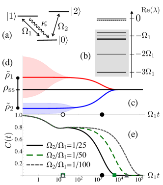
Example I: 3-level system. Consider the 3-level system of Fig. 1(a), with Hamiltonian and jump operator . When , dynamics can be “shelved” for long times in , giving rise to intermittency in quantum jumps Plenio and Knight (1998), which can be seen as coexistence of “active” and “inactive” dynamical phases Garrahan and Lesanovsky (2010). Figure 1(b) shows the spectrum of : the gap is small for , the two leading eigenvalues detach from the rest (i.e., ), and the dynamics is metastable. Figure 1(c) illustrates the trace distance of the state to the MM starting from : an initial decay on times of order of to the nearest point on the MM (in this case to an eMS) is followed by decay to on times of order (since ). The MM for this case is a one-dimensional simplex (i.e., a convex set whose interior points uniquely represent probability distributions on the vertices), see Fig. 1(d).
For the convex set MM of possible coefficients can have more than extreme points. For classical dynamics it has been proven that this set is well approximated by a simplex Gaveau and Schulman (2006), whose vertices correspond to disjoint eMS and its barycentric coordinates to the probabilities of a metastable state decomposed as a mixture of the eMS, cf. Fig. 1(d). For quantum dynamics and , we expect the structure of the MM to be richer than just a simplex. As we describe below, the MM can in general also include decoherent free subspaces (DFS) Zanardi and Rasetti (1997); Zanardi (1997); Lidar et al. (1998) and noiseless subsystems (NSS) Knill et al. (2000); Zanardi (2000) which are protected from dissipation in the metastable regime, as the next example shows.
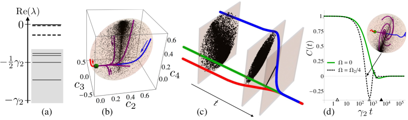
Example II: Collective dissipation and a metastable DFS. Consider a two-qubit system with Hamiltonian , and a collective jump operator . When there is a small gap and the four leading eigenvalues of detach from the rest, Fig. 2(a). This is related to the fact that any superposition of and is annihilated by . Fig. 2(b) maps out the MM by randomly sampling all (pure) initial states from and obtaining their corresponding metastable state via Eq. (4): the MM is an affinely transformed Bloch ball corresponding to a DFS qubit within the metastable regime . It important to note: (i) this coherent structure is not the consequence of a symmetry, as for the system dynamics neither has a U(2) nor an up-down nor a permutation symmetry, cf. Albert and Jiang (2014); (ii) the smallest for which we can obtain a DFS is , as in this case.
Structure of metastable manifold. We aim to find the general structure of the MM for two classes of systems for which has a small gap: (A) finite systems where the gap closes at some limiting values of the parameters in (such as in Example I, and in Example II); (B) scalable systems of size where the gap closes only in the thermodynamic limit (such as the dissipative Ising model of Ref. Ates et al. (2012)).
For class A we prove via non-Hermitian degenerate perturbation theory Note (5) that the structure of a metastable state is given by the following block structure,
| (6) |
with being the orthogonal sum , where are fixed states on (cf. eMS above), are arbitrary states on , and are probabilities. Up to the corrections, this is a general structure of a manifold of stationary states of open quantum Markovian dynamics Baumgartner and Narnhofer (2008). The metastable regime is given by where is the relaxation time for the unperturbed dynamics and is the scale of the perturbation Note (5). The corrections in Eq. (6) are of the order of the corrections to the invariance of the MM during the metastable time regime, cf. Eq. (14). The coefficients that determine , see Eq. (4), correspond approximately to an affine transformation of the entries of () in Eq. (6) with Note (5). Therefore, the MM approximately represents the degrees of freedom of the classical-quantum space in Eq. (6).
For class B we conjecture that the coefficients representing the MM converge to degrees of freedom of a classical-quantum space as in Eq. (6), when the separation in the spectrum becomes more and more pronounced as . Note that the dimensionality of the MM does not change with and thus the convergence is well defined. This general conjecture is based on the necessary condition that the low-lying spectrum of features only trivial Jordan blocks 666Non-trivial Jordan blocks would lead to an unbounded norm of in the limit of Wolf (2012). More precisely, Jordan blocks may be considered as long as they do not contribute significantly, so that Eq. (14) holds true with appropriately redefined corrections being small. This condition aims to exclude systems where a small gap is “accidental” in the sense it is unrelated to it vanishing in some limit. . Note that a conjecture of the structure being approximately that of stationary states, cf. Eq. (6), is a stronger claim. A proof of the former conjecture for class B appears challenging at this moment, see comment in Note (5).
The blocks in Eq. (6) can be of three kinds: (i) When , the -th block is a disjoint eMS. This is the case in Example I, where there are two eMS, , with metastable states being mixtures of them. For classical systems the MM is always approximately a simplex of disjoint eMS Gaveau and Schulman (2006) with probabilities representing classical degrees of freedom. (ii) When and , is a decoherence free subspace (DFS) protected from the noise. This is the case in Example II where the MM is a qubit. (iii) When and , is also protected from noise and termed a noisless subsystem (NSS). The structures (ii) and (iii) correspond to quantum degrees of freedom () and do not appear in the case of classical dynamics Gaveau and Schulman (2006). In general the number of blocks in Eq. (6) is , with equality occurring only when there are no DFS or NSS.
Effective motion in the metastable manifold. In the metastable regime, , metastable states appear stationary, or perhaps rotate within the MM. This latter case corresponds to either: (i) coherent motion in the DFS/NSS where the matrices of Eq. (6) evolve unitarily in time; or (ii) classical rotations with a frequency which is limited by the dimensionality of MM 777This latter classical motion was not considered in Gaveau and Schulman (2006), as the low-lying eigenvalues of were assumed all real. One can show Macieszczak et al. that the set of is again a simplex. Points within the simplex evolve within it. Due to exponential shrinking, this evolution can allow for rotations, but with limited frequencies which decrease with decreasing gap.. For class A systems only case (i) is possible Note (5); Zanardi and Campos Venuti (2014, 2015).
For longer times, , the MM contracts exponentially towards . This is illustrated in Fig. 2(c) for Example II. This low dimensional evolution in the MM is well described by an effective generator , which can be considered as the generator of the dynamics averaged over intervals . If the MM is approximately a simplex (i.e., containing no DFS or NSS) the motion generated by is that of classical transitions between macrostates described by the eMS (see Note (5) for and Macieszczak et al. for the general case). For class A when the MM contains coherent subsystems/subspaces, the motion preserves the structure of Eq. (6) and can be shown to be trace-preserving and approximately completely-positive Note (5); Zanardi et al. (2016); Cai and Barthel (2013). Note that decoupling of (slower) classical dynamics from (faster) quantum evolution in the MM requires further separation in low-lying eigenvalues of . This is illustrated in Fig. 2(c) for Example II.
In practice, metastability can be accessed through the connected auto-correlation Sciolla et al. (2015) of the measurement of a system observable, even in the stationary state, 888 For an observable , we have that .; see Figs. 1(e), 2(d). The first measurement perturbs , and the state conditioned on the result partially relaxes towards the MM for . In the metastable regime correlations will persist as the different blocks in (6) do not communicate, and for the case where all low-lying eigenvalues are real, . When low-lying eigenvalues are complex, oscillations of can occur in the metastable regime, as in Fig. 2(d). When , dynamics begins to relax back towards , erasing all information about the initial result, , for .
Outlook. The next steps in the development of the theory of quantum metastability presented here include:
(i) For many-body systems, where direct diagonalisation of is impractical, it should be possible to use dynamical large-deviation methods Touchette (2009) to identify dynamically the different blocks in Eq. (6) by biasing ensembles of quantum trajectories Garrahan and Lesanovsky (2010). This approach could be implemented numerically by generalising classical path sampling Hedges et al. (2009) and/or cloning techniques Giardina et al. (2011).
(ii) In order to reveal the structure of the MM, one needs to find a general computational scheme that can identify the basis in which metastable states look explicitly as in Eq. (6). Such a method would be useful to uncover DFS and NSS more generally. Also, it would be interesting to consider more broadly DFS that do no arise as a consequence of symmetry, cf. Example II above.
(iii) We have considered here metastability in the case of Markovian dynamics generated by a Lindbladian . Metastability occurs also when dynamics is non-Markovian, see e.g. Merkli et al. (2015). It should be possible to generalise the method introduced above to the non-Markovian case of a time-dependent generator .
(iv) A significant challenge is to extend the ideas presented here to study metastability in closed quantum systems. This would be relevant to the fundamental problems of thermalisation Eisert et al. (2014) and many-body localisation Nandkishore and Huse (2015).
Acknowledgements.
This work was supported by EPSRC Grant No. EP/J009776/1 and ERC Grant Agreement No. 335266 (ESCQUMA). K.M. thanks M. Idel for discussions.References
- Binder and Kob (2011) K. Binder and W. Kob, Glassy Materials and Disordered Solids (World Scientific, 2011).
- Biroli and Garrahan (2013) G. Biroli and J. P. Garrahan, J. Chem. Phys. 138, 12A301 (2013).
- Berthier and Ediger (2016) L. Berthier and M. D. Ediger, Physics Today 69, 40 (2016).
- Polkovnikov et al. (2011) A. Polkovnikov, K. Sengupta, A. Silva, and M. Vengalattore, Rev. Mod. Phys. 83, 863 (2011).
- Eisert et al. (2014) J. Eisert, M. Friesdorf, and C. Gogolin, Nature Physics 11, 7 (2014).
- (6) L. D’Alessio, Y. Kafri, A. Polkovnikov, and M. Rigol, arXiv:1509.06411 .
- Gogolin and Eisert (2016) C. Gogolin and J. Eisert, Reports on Progress in Physics 79, 056001 (2016).
- Nandkishore and Huse (2015) R. Nandkishore and D. A. Huse, Annu. Rev. Condens. Matter Phys. 6, 15 (2015).
- (9) N. Y. Yao, C. R. Laumann, J. I. Cirac, M. D. Lukin, and J. E. Moore, arXiv:1410.7407 .
- De Roeck and Huveneers (2014) W. De Roeck and F. Huveneers, Phys. Rev. B 90, 165137 (2014).
- Prosen (2011) T. Prosen, Phys. Rev. Lett. 106, 217206 (2011).
- Markland et al. (2011) T. E. Markland, J. A. Morrone, B. J. Berne, K. Miyazaki, E. Rabani, and D. R. Reichman, Nature Phys. 7, 134 (2011).
- Olmos et al. (2012) B. Olmos, I. Lesanovsky, and J. P. Garrahan, Phys. Rev. Lett. 109, 020403 (2012).
- Sciolla et al. (2015) B. Sciolla, D. Poletti, and C. Kollath, Phys. Rev. Lett. 114, 170401 (2015).
- van Horssen et al. (2015) M. van Horssen, E. Levi, and J. P. Garrahan, Phys. Rev. B 92, 100305 (2015).
- Znidaric (2015) M. Znidaric, Phys. Rev. E 92, 042143 (2015).
- Zanardi and Rasetti (1997) P. Zanardi and M. Rasetti, Phys. Rev. Lett. 79, 3306 (1997).
- Zanardi (1997) P. Zanardi, Phys. Rev. A 56, 4445 (1997).
- Lidar et al. (1998) D. A. Lidar, I. L. Chuang, and K. B. Whaley, Phys. Rev. Lett. 81, 2594 (1998).
- Kielpinski et al. (2001) D. Kielpinski, V. Meyer, M. Rowe, C. Sackett, W. Itano, C. Monroe, and D. Wineland, Science 291, 1013 (2001).
- Knill et al. (2000) E. Knill, R. Laflamme, and L. Viola, Phys. Rev. Lett. 84, 2525 (2000).
- Zanardi (2000) P. Zanardi, Phys. Rev. A 63, 012301 (2000).
- Viola et al. (2001) L. Viola, E. M. Fortunato, M. A. Pravia, E. Knill, R. Laflamme, and D. G. Cory, Science 293, 2059 (2001).
- Nielsen and Chuang (2000) M. A. Nielsen and I. Chuang, Quantum Information. Cambridge University Press, Cambridge (2000).
- Gaveau and Schulman (1996) B. Gaveau and L. S. Schulman, J. Mat. Phys. 37, 3897 (1996).
- Gaveau and Schulman (1998) B. Gaveau and L. S. Schulman, J. Mat. Phys. 39, 1517 (1998).
- Gaveau and Schulman (1999) B. Gaveau and L. S. Schulman, J. Phys. A 20, 2865 (1999).
- Bovier et al. (2002) A. Bovier, M. Eckhoff, V. Gayrard, and M. Klein, Comm. Math. Phys 228, 219 (2002).
- Gaveau and Schulman (2006) B. Gaveau and L. S. Schulman, Phys. Rev. E 73 (2006).
- Nicholson et al. (2013) S. Nicholson, L. Schulman, and E. Kim, Phys. Lett. A 377, 1810 (2013).
- (31) J. Kurchan, arXiv:0901.1271 .
- Lindblad (1976) G. Lindblad, Comm. Math. Phys 48, 119 (1976).
- Gorini et al. (1976) V. Gorini, A. Kossakowski, and E. C. G. Sudarshan, J. Mat. Phys. 17, 821 (1976).
- Plenio and Knight (1998) M. B. Plenio and P. L. Knight, Rev. Mod. Phys. 70, 101 (1998).
- Gardiner and Zoller (2004) C. Gardiner and P. Zoller, Quantum noise (Springer, 2004).
- Note (1) Calligraphic font denotes super-operators, such as the generator , while Roman font denotes normal operators, such as the Hamiltonian or the jump operators .
- Note (2) and are right and left eigenmatrices of for eigenvalue , i.e., and . In principle since in general . Left and right eigenmatrices form a complete basis, which we normalise as . We assume there are no Jordan blocks in the part of the spectrum relevant for our analysis; see e.g. Ref. Gaveau and Schulman (2006).
- Note (3) The norm of a super-operator , is the norm induced by the trace norm, , of complex matrices on which acts: .
- Note (4) For real eigenvalues, and can be chosen Hermitian. Note that while , are not positive. Complex eigenvalues come in conjugate pairs and if so we have , .
- Note (5) See Supplemental Material for derivations of (i) case : approximate disjointness of two EMSs and the effective classical dynamics. (ii) class A systems: the structure of the metastable manifold from Eq. (6), the metastable regime and the effective dynamics. (iii) class B systems: a comment on the conjecture.
- Garrahan and Lesanovsky (2010) J. P. Garrahan and I. Lesanovsky, Phys. Rev. Lett. 104, 160601 (2010).
- Albert and Jiang (2014) V. V. Albert and L. Jiang, Phys. Rev. A 89, 022118 (2014).
- Zanardi and Campos Venuti (2014) P. Zanardi and L. Campos Venuti, Phys. Rev. Lett. 113, 240406 (2014).
- Zanardi and Campos Venuti (2015) P. Zanardi and L. Campos Venuti, Phys. Rev. A 91, 052324 (2015).
- Ates et al. (2012) C. Ates, B. Olmos, J. P. Garrahan, and I. Lesanovsky, Phys. Rev. A 85, 043620 (2012).
- Baumgartner and Narnhofer (2008) B. Baumgartner and H. Narnhofer, J. Phys. A 41, 395303 (2008).
- Note (6) Non-trivial Jordan blocks would lead to an unbounded norm of in the limit of Wolf (2012). More precisely, Jordan blocks may be considered as long as they do not contribute significantly, so that Eq. (14\@@italiccorr) holds true with appropriately redefined corrections being small. This condition aims to exclude systems where a small gap is “accidental” in the sense it is unrelated to it vanishing in some limit.
- Note (7) This latter classical motion was not considered in Gaveau and Schulman (2006), as the low-lying eigenvalues of were assumed all real. One can show Macieszczak et al. that the set of is again a simplex. Points within the simplex evolve within it. Due to exponential shrinking, this evolution can allow for rotations, but with limited frequencies which decrease with decreasing gap.
- (49) K. Macieszczak, M. Guta, I. Lesanovsky, and J. P. Garrahan, in preparation .
- Zanardi et al. (2016) P. Zanardi, J. Marshall, and L. Campos Venuti, Phys. Rev. A 93, 022312 (2016).
- Cai and Barthel (2013) Z. Cai and T. Barthel, Phys. Rev. Lett. 111, 150403 (2013).
- Note (8) For an observable , we have that .
- Touchette (2009) H. Touchette, Phys. Rep. 478, 1 (2009).
- Hedges et al. (2009) L. O. Hedges, R. L. Jack, J. P. Garrahan, and D. Chandler, Science 323, 1309 (2009).
- Giardina et al. (2011) C. Giardina, J. Kurchan, V. Lecomte, and J. Tailleur, J. Stat. Phys. 145, 787 (2011).
- Merkli et al. (2015) M. Merkli, H. Song, and G. P. Berman, J. Phys. A 48, 275304 (2015).
- Rosmanis (2012) A. Rosmanis, Linear Algebra and its Applications 437, 1704 (2012).
- Wolf (2012) M. M. Wolf, Quantum channels and operations: Guided tour (2012).
Supplemental Material
Metastability for two low-lying eigenmodes
Here we consider the case of low-lying eigenvalues in the master operator , see Eqs. (1-4) in the main text.
Since the metastable manifold (MM) is convex and 1-dimensional, it is simply an interval and thus a simplex. Hence, any metastable state is a mixture of extreme metastable states (eMSs), in this case two: , . As a metastable state, , is determined by the coefficient , the eMSs correspond to the extreme values of given by the maximum and minimum eigenvalue of , see Eq. (5) in the main text. Furthermore, note that , are the metastable states for the pure initial state given by the eigenvectors corresponding to and , respectively. As are then given by the truncated evolution equation (3) of the main text, we have and are approximately positive with the corrections bounded by the corrections to stationarity in the metastable regime.
The decomposition of a metastable state into the eMSs is given by the observables , (for definition see the main text below Eq. (5)) which determine the probabilities as . We note that the definition of and insures that for , and and , i.e., constitute a POVM.
Approximate disjointness of two eMS. Below we prove that the extreme metastable states are approximately disjoint. More precisely, we show that there is a division of the system Hilbert space so that , where are the corrections to the stationarity in the metastable regime, cf. Eq. (3) in the main text.
Proof. Note that the stationary state is a mixture of the two eMS, , where and . We define the orthogonal subspaces and as follows,
| (7) | |||||
| (8) |
where is the orthonormal eigenbasis of , which is also the eigenbasis of both and . From , we have . Let and denote the eigenvectors of corresponding to the extreme eigenvalues and . Let , further be the system state at time for the initial state chosen as ,. From the orthogonality of the eigenmatrices of (also in the case of Jordan blocks in ), it follows that
| (9) |
From positivity of and the fact that is diagonal in the eigenbasis of , we also have
| (10) |
Together with Eq. (9) it follows that
| (11) |
where are the corrections to the stationarity in the metastable regime, cf. Eq. (3). Analogously, , which ends the proof. Let us note that this argument is analogous to the case of in classical systems g2 .
Effective classical dynamics in the metastable manifold. Here we consider the linear operator which governs the dynamics for times . Note that in this case, , we have simply .
Note that by the construction, the operator transforms the MM into itself. As for the MM is a simplex, generates a positive and probability preserving evolution of the probabilities . This implies that is a generator of classical stochastic dynamics. Indeed, in the basis of extreme metastable states, , , we have
| (12) |
where . We have that and due to . Therefore it follows that indeed obeys the generator characteristics: the diagonal terms are negative, the off-diagonal terms are positive and the sum of entries in each column is 0. The corresponding dynamics is thus given by
| (13) |
and for we obtain the probabilities corresponding to the stationary state, . The dynamics in (13) approximates the system dynamics with the corrections being bounded by the corrections to stationarity in the metastable regime (cf. Eq. (2) in the main text),
| (14) |
Let us finally emphasize that for times dynamics takes place between eMSs, , , which can be considered as system macrostates in analogy to classical thermodynamics. The generator in Eq. (12) yields stochastic trajectories of transitions between , . Those trajectories correspond to quantum trajectories coarse-grained in time over intervals of the order , similarly as in the example of 3-level atom, see Fig. 1 in the main text, the intermittency in quantum jumps corresponds to conditional system dynamics being restricted to the dark level (“inactive” dynamics) or the subspace spanned by the level and (“active” dynamics) M .
Characterising the structure of the metastable manifold and effective dynamics for Class A systems
In this section we discuss metastablity of a finite open quantum system for which the gap closes at some value of parameters in the master equation (see Eq. (1) in the main text) so that the stationary state is no longer unique. For dynamics which are close to the degenerate case, we prove that there is a separation in the spectrum leading to a metastable time regime during which the system’s state has the structure given in Eq. (6) of the main text. Moreover, the effective dynamics in the metastable manifold is trace-preserving and approximately completely positive.
Perturbation theory analysis. We use the perturbation theory of linear operators (see Chapter 2 of K95 ) in order to analyse an open quantum system of finite dimension whose Lindblad operator is obtained by perturbing a generator featuring multiple stationary states. We consider with -fold degeneracy of the stationary state manifold (SSM). In the proof we assume that the dynamics exhibits no rotations in the stationary state manifold, i.e. has no non-zero imaginary eigenvalues. The case of unitarily rotating SSM can be analysed in a similar fashion M . Consequently, there are right (left) eigenmatrices corresponding to the eigenvalues, with no non-trivial Jordan blocks due to positive and trace-preserving dynamics W . The asymptotic states of have the structure given by Eq. (6) in the main text (without the corrections), see e.g. B08 . We denote by the projection on the SSM of , with , so that for the initial state , the asymptotic state is given by and , .
For simplicity, we consider a linear perturbation of the Hamiltonian , where is Hermitian, and of the jumps operators are . The derivations below can be easily generalised to any analytic perturbation of and K95 . This leads to the following first- and second-order perturbation for the generator
| (15) |
We choose the dimensionless scale parameter so that that , where is the relaxation time for dynamics (see below Eqs. (16)-(Characterising the structure of the metastable manifold and effective dynamics for Class A systems) for the precise definition of ).
From the perturbation theory of linear operators K95 , the eigenvalues of the perturbed operator are continuous with respect to . Furthermore, if is an eigenvalue of with algebraic multiplicity , then for small enough eigenvalues of will cluster around the unperturbed eigenvalue . Those eigenvalues are referred to as the -group. In general the individual eigenvalues in the -group are not analytic in , but correspond to branches of analytic functions. Moreover, the corresponding eigenmatrices may feature poles. However, the projection onto the subspace spanned by the -group eigenmatrices is analytic and it follows that the restriction of to this subspace is analytic as well. When , the eigenvalue and the projection on the corresponding eigenmatrix is analytic.
In particular, for small enough, the first eigenvalues of belong to -group clustering around and the separation to the -th eigenvalue is maintained. Let be the analytic projection on the -group, (which is denoted by in the main text for a generic system). Then the restricted generator is given by . Since there are no non-trivial Jordan block associated with the -eigenvalue of W , we have K95
| (16) | |||||
where is the reduced resolvent of at , i.e. and . The resolvent is related to the relaxation time, . We now define the scale of the perturbation in Eq. (15) so that , and we will make repeated use of this bound below.
Spectrum of . As we show below, from the fact that both and are completely positive trace-preserving (CPTP) generators, it follows that first -eigenvalues of are not only continuous, but differentiable continuously at least twice, i.e.,
| (18) |
Moreover, we have that and , so that the spectrum structure of a positive trace-preserving generator is reproduced in the second order of the perturbation theory. This is due to the fact that the first-order correction is an eigenvalue of , which is a unitary generator Z1 ; Z2 and the second-order correction is an eigenvalue of a CPTP generator on the SSM of (see also Z3 ).
In the generic case when the degeneracy of the first -eigenvalues is lifted in the second order of the perturbation theory, we further demonstrate that all are actually analytic in and so are the projections on the corresponding eigenmatrices, . Note that in this case, the stationary state of for is necessary unique, as considered in the main text.
First-order perturbation. Let . As we show at the end of this section is a CPTP generator on the SSM of , and thus its eigenvalues have non-positive real parts. From the definition of we see that also is a CPTP generator, but its first-order correction is of the opposite sign. Hence, eigenvalues must be imaginary and there is no dissipation. Indeed, in Z1 ; Z2 it was shown that the first order yields unitary dynamics and the formula for the corresponding Hamiltonian was derived.
Second-order perturbation. Let The generator lifts partially the degeneracy of the -eigenvalues. From Eq. (Characterising the structure of the metastable manifold and effective dynamics for Class A systems), analogously as in the Hermitian perturbation theory, in order to further lift the degeneracy the higher-order corrections should be considered separately for each eigenprojection of . This corresponds to the reduction process K95 in which, instead of , one equivalently considers the perturbation theory for with the unperturbed operator and an analytic perturbation, cf. Eq. (Characterising the structure of the metastable manifold and effective dynamics for Class A systems). The eigenvalues of are related to , …, of simply be multiplication by . Since the unitary generator features only trivial Jordan blocks, for the eigenspace related to its eigenvalue we obtain that (cf. Eqs. (16), (Characterising the structure of the metastable manifold and effective dynamics for Class A systems))
| (19) | |||||
| (20) | |||||
Above, denotes the projection on the -eigenspace of , so that we have . Also, is the projection on the -group and is the reduced resolvent for at , restricted to . Finally, (inv.) denotes the terms with the inverted order of operators.
From Eq. (20) we see that the degeneracy of the eigenvalues can be further lifted by the operator . Due to the reduction process the eigenvalues of from -group are of the form , where is an eigenvalue of and is the corresponding eigenvalue of (see Eq. (39)). Below we show that , which ends the proof of Eq. (18). Moreover, when the eigenvalues of are non-degenerate, the corresponding perturbed eigenvalues, , are analytic in and thus the -group eigenvalues of are analytic. Furthermore, the projection on the eigenmatrix corresponding to is analytic and since it is also a projection on the eigenvalue from the -group, the projections on the low-lying eigenvalues of are analytic.
We argue now that . We use the fact proven at the end of this section that is a CPTP generator on the SSM of . The restricted operator can be related to as follows,
| (21) |
Note that is the interaction picture for . Hence it is a CPTP generator on the SSM of and as an integral of CPTP generators is also a CPTP generator on the SSM. Moreover, the eigenvalues of obey , which ends the proof. Note that Eq. (21) is the first-order perturbation theory for weak dissipation, where the fast unitary evolution given by erases all the contributions of the slow dissipation that would create any coherence with respect to the eigenbasis of the Hamiltonian governing the unitary evolution.
Time regime of metastability. We now discuss how the perturbations in Eq. (15) change the system dynamics. We derive the metastable regime when the system dynamics appears stationary as a consequence of the separation in the spectrum of discussed above. Let us consider separately the low-lying modes, given by the projection , and the rest of modes (cf. Eq. (2) in the main text)
| (22) |
Timescale . By definition, the dynamics maps the MM defined by into itself. However, in the metastable regime, the system dynamics leaves the MM approximately invariant, in the sense that its image is well approximated by the MM itself. This defines the longer timescale of the regime (see the main text). As the first-order correction to in Eq. (Characterising the structure of the metastable manifold and effective dynamics for Class A systems) corresponds to the unitary dynamics leaving the SSM of invariant, the timescale will be related to higher-order corrections in , , cf. Eq (16). Indeed, below we show that the corrections to the invariance of the MM are given by
The first line describes unitary dynamics in the metastable manifold, whereas the second line is the contribution from the dissipative dynamics (in the interaction picture). Therefore, the metastable regime is limited to times for which all three terms on the second line are small. Since terms are bounded by , and respectively the condition is satisfied if , where
| (24) | |||||
Here we used Eq. (Characterising the structure of the metastable manifold and effective dynamics for Class A systems) and the definition of the scaling to conclude that , and the Taylor expansion in the first line. Note that for small the leading term of the metastable range is .
Derivation of Eq. (Characterising the structure of the metastable manifold and effective dynamics for Class A systems). The proof below is analogous to the results of the appendix in Z2 . Note that for times the unitary contribution to the dynamics, , cannot be neglected (see also Z1 ). In order to derive the perturbation series in for , we consider the Dyson expansion
| (25) |
where of the order is treated as the perturbation to inside . Using in Eq. (16) and we obtain
where the higher-order corrections are explained below. First, as both and are CPTP generators and for positive and trace-preserving W05 , we have and . The first line in Eq. (Characterising the structure of the metastable manifold and effective dynamics for Class A systems) corresponds to and the higher-order corrections are of the order due to the norm being submultiplicative, see reference [36] in the main text. Furthermore, the corrections in the second line, which corresponds to the integral term in (25), are of the order
where is the third-order correction in (see Eq. (37)). Furthermore, since we also have
and further
where we have used the Dyson expansion for , see Eq. (25), with corrections being the integral and the unitary evolution outside the SSM given by (the first line in (25)). Finally, we note that (cf. Eq. (Characterising the structure of the metastable manifold and effective dynamics for Class A systems)), and (cf. Eq. (37))), which completes the proof of Eq. (Characterising the structure of the metastable manifold and effective dynamics for Class A systems).
Timescale . The metastable regime begins when the contribution from the fast decaying modes corresponding to the eigenvalues , , …, becomes negligible and the initial relaxation to the low-lying modes takes place. The timescale in the decay of this contribution of the order is derived below as
| (27) |
Derivation. Consider the Dyson expansion for
| (28) |
where is considered as a perturbation of , cf. Eq. (15). As both and are CPTP generators, we have W05 . Using the expression (16) for , we obtain
In the first line we used the multiplicativity of the norm, and . In the second line we bound the integral in Eq. (28) by we arrive at the correction .
We now use the following definition of the relaxation time, as the shortest timescale such that for any initial state , the system state relaxes to the stationary state as , which implies . From Eq. (Characterising the structure of the metastable manifold and effective dynamics for Class A systems) we get
| (30) | |||||
Note that the correction for times is of the same order as the leading corrections to the invariance of the MM, cf. Eq. (Characterising the structure of the metastable manifold and effective dynamics for Class A systems), and hence does not determine the timescale of the initial relaxation. Therefore, for times , the contribution from the fast decaying modes is a sum of terms of the order and of the same order as the corrections to the invariance of the MM. Similar results would be obtained for defined so that , where is that gives the supremum.
Furthermore, in the situation when , i.e., when there are not too many modes contributing to the system dynamics, and is non-degenerate, we have (see Eq. (Characterising the structure of the metastable manifold and effective dynamics for Class A systems))
Structure of the metastable manifold. We consider now the projection of an evolved initial state onto the metastable manifold (MM) defined by . Using the results (Characterising the structure of the metastable manifold and effective dynamics for Class A systems) and (27) for the timescales and respectively we find that in the metastable regime the system state is approximated by (see Eq. (3) and (4) in the main text)
| (31) |
where the imaginary parts of the low-lying eigenvalues are given in the first order by the unitary dynamics within the MM (see Eqs. (16) and (Characterising the structure of the metastable manifold and effective dynamics for Class A systems)). As is the projection on the SSM of , is approximately of the form given by Eq. (6) in the main text with the correction . Furthermore, this correction is of the same order as the corrections to invariance of the MM, i.e., the dissipative dynamics, for times within the metastable regime , see the second line in Eq. (Characterising the structure of the metastable manifold and effective dynamics for Class A systems) and Eqs. (24) and (27).
Coefficients of the MM. Let us consider the generic case when the degeneracy of the first eigenvalues of is lifted in the second-order perturbation theory. In this case the projections on the individual eigenmatrices are analytic and so are the coefficients of the MM, . Moreover, , ,…, and , , …, correspond to the eigenbasis of (cf. Eq. (21)) and thus constitute a basis of the SSM of . Thus, for small enough, the set of coefficients representing the MM is well approximated by the image of an affine transformation of the degrees of freedom describing the SSM of , i.e. the entries of the DFS/NSS states, , , with the condition (cf. Eq. (6) of the main text). That affine transformation is determined by to the linear transformation between the basis of the SSM of the entries in , to , , …, .
Derivation. In the section on the spectrum of , we argued that when the degeneracy is lifted in the second order, for small enough, the first eigenvalues of are analytic. Moreover, the eigenvalues are of the form , where is an eigenvalue of with corresponding projection , and is an eigenvalue of . Due to the reduction process, the higher-order corrections correspond to the perturbation theory for with the unperturbed operator and an analytic perturbation. The first (third)-order perturbation is given by Eq. (39). We thus have (cf. Eq. (19))
| (32) |
where is the projection on the eigenmatrix corresponding to the eigenvalue of , is the reduced resolvent for at restricted to , and is the reduced resolvent for at restricted to . Note that the corrections depend via and on the way the degeneracy is lifted inside the SSM in the first and the second order of the perturbation theory. The right eigenvector corresponding to is thus proportional to
where is the left eigenmatrix of corresponding to . Note that since the projection is of rank 1, the eigenmatrix can be replaced by any matrix such that . Let us assume is Hermitian (see the paragraph with Eq. (4) in the main text), so that the coefficient is real.
Consider normalised in the spectral norm , which corresponds to the maximal absolute value of the eigenvalues. Note that . From the Hermitian perturbation theory for , the eigenvalues of are analytic K95 , but does not have to be differentiable at , which happens when the extreme eigenvalues of obey . Nevertheless, for a given sign of , is analytic for small enough. Therefore, we arrive at
| (33) |
where we assumed and related to the first-order correction to or with its sign depending on the sign of . Therefore, for small enough the set of coefficients representing the MM is simply an affine transformation of the degrees of freedom of the SSM of as given in Eq. (6) of the main text.
Consider an alternative case in which the coefficient is ”normalised” by the difference of the extreme eigenvalues of , . This ”normalisation” is convenient as the range of all coefficients determining the MM is of the same length , which is also the case for probabilities in a simplex or a Bloch ball, see Fig. 2. in the main text. From the Hermitian perturbation theory for we have that is analytic in and thus
| (34) |
where we assumed and is the difference between first-order corrections in and .
Effective dynamics in the metastable manifold. Previously we showed that the dynamics in the metastable regime is approximated by unitary transformation of the MM with generator . Here we show that for times (i.e. following the metastable regime) the dynamics in the MM is dissipative and is characterised by the CPTP generator on the SSM of . In particular, we prove that
| (35) |
We note that dynamics generated in the SSM by was previously discussed in Z3 for the special case of a Hamiltonian perturbation (see Eq. (15)) and .
Proof. Note that from the fact that is trace-preserving, it follows that it features the left eigenmatrix corresponding to -eigenvalue, which, by construction, also holds true for . Therefore, is trace-preserving.
From Eq. (Characterising the structure of the metastable manifold and effective dynamics for Class A systems) we write , with regarded as a perturbation whose size is in general , while in the case when we have , see the third-order correction for in Eq. (37). The Dyson expansion for with as the perturbation is
where we used . We further have
Note that since is a CPTP generator on . Due to submultiplicativity of the norm, the corrections to in the first line are . In the second line corresponding to the integral term, the corrections are bounded by . From Eq. (Characterising the structure of the metastable manifold and effective dynamics for Class A systems) we get which implies that the leading correction in the second line is .
Stationary state. We note that a stationary state of the dynamics perturbed away from the degeneracy have been studied in B08 . In the case when the degeneracy is lifted in the second order of the perturbation theory, we have that (cf. Eq. (32))
| (36) |
where is the unique stationary state of the generator in Eq. (21). Let denote the projection on the ()-eigenspace of . is the reduced resolvent of at , restricted to , is the third-order perturbation in the reduction process for eigenspace , see Eq. (39), and is the resolvent of , restricted to . Note that from the orthonormality of the eigenbasis of the CPTP generator (the first and second order of perturbation theory for ), we further have for any matrix , where , and thus .
Proof of the CPTP property of the effective generator. We now prove that and generate CPTP dynamics on the SSM given by . We use Theorem 3.17 from D80 on convergence of one-parameter semigroups, whose statement we recall here for the special case of finite dimensional spaces. Let , be generators of one-parameter semigroups , on a Banach space , and assume that for each in a spanning set of there exist such that and . Then for all the limit , where is the norm in .
Proof for . To prove the CPTP property consider , where is an orthonormal basis of the system space . We choose and so that is the Choi matrix for . By choosing appropriate CPTP generators and matrices we will show that is a limit of Choi matrices of quantum channels. Thus for all , is positive and , where denotes the partial trace over the first subsystem in , and consequently generates CPTP dynamics on the SSM given by . To prove this, we choose , which is a CPTP generator on as is a generator of unitary quantum dynamics. By defining , where and , we arrive at the conditions of the theorem 3.17 in D80 with the norm being the trace norm (see [36] in the main text). We note that the generator property of was previously discussed in Z3 for the special case of the Hamiltonian perturbation (see Eq. (15)) and .
Proof for . Similarly, to prove that generates CPTP dynamics on the SSM given by , we need to choose and . By considering and we arrive at the conditions of the theorem 3.17 in D80 . We note that was proven to be a unitary generator in Z1 ; Z2 .
Expressions for higher-order corrections and . We have that , where and are given in Eq. (Characterising the structure of the metastable manifold and effective dynamics for Class A systems) and the third-order correction is K95
| (37) | |||||
| (38) | |||||
Due to reduction process for we further obtain that , where is a projection on the -group with being an eigenvalue of and
| (39) | |||||
Comment on the conjecture for Class B
For class B a proof of our conjecture of the MM structure appears difficult.
The convex analysis tools used in the classical proof g1 ; g2 ; g3 ; g4 cannot be used for the quantum case as they rely on the finite number of pure states of a finitely-dimensional classical system. Note, however, that by using any tools of convex analysis for the MM represented by the set of coefficients , and exploiting (approximate) positivity of the metastable states, one could at most prove the structure of fixed points of positive (cf. completely positive) maps I13 , which is richer than Eq. (6). For example, for there can exist non-commuting eMS ( real Hermitian matrices) in contrast to for a smallest DFS/NSS of a qubit. In order to exploit complete positivity one would need to work with the dynamics extended to , which has low-lying eigenvalues and thus the simplicity of the geometric representation of the MM is lost.
For the stronger conjecture determining also the structure of the metastable states, the difficulty lies in the fact that the existing proof of the SSM structure relies on the property that eigenmatrices corresponding to strictly zero eigenvalue of a CPTP generator (or the eigenvalue 1 of a CPTP quantum channel) form a von-Neumann algebra and thus are of the form given in Eq. (6) of the main text B08 ; W . We cannot rely on the algebra structure of metastable states as for states with approximately the block structure, this structure will not be preserved with the same approximation for products of them. This corresponds to the corrections to complete positivity of the dynamics (of the same order as the corrections to the stationarity, cf. Eq. (3)) being progressively accumulated with each multiplication of the eigenmatrices (cf. the proof of the SSM structure in W ). It is likely one could use a proof such as in R12 deriving Eq. (6) by exploiting properties of a projection on steady states without its multiple applications.
These points will be elaborated further in M .
References
- (1) B. Gaveau and L. S. Schulman, J. Mat. Phys. 39, 1517 (1998).
- (2) K. Macieszczak, M. Guta, I. Lesanovsky, and J. P. Garrahan, in preparation.
- (3) T. Kato, Perturbation Theory for Linear Operators (Springer, 1995).
- (4) M. M. Wolf, Quantum channels and operations: Guided tour (2012).
- (5) B. Baumgartner and H. Narnhofer, J. Phys. A 41, 395303 (2008).
- (6) P. Zanardi and L. Campos Venuti, Phys. Rev. Lett. 113, 240406 (2014).
- (7) P. Zanardi and L. Campos Venuti, Phys. Rev. A 91, 1 (2015).
- (8) P. Zanardi, J. Marshall and L. Campos Venuti, Phys. Rev. A 93, 022312 (2016).
- (9) J. Watrous, Quantum Inf. Comput. 5, 58 (2005).
- (10) E. B. Davies, One-parameter semigroups (Academic Press, 1980).
- (11) A. Rosmanis, Linear Algebra and its Applications 437, 1704 (2012).
- (12) B. Gaveau and L. S. Schulman, J. Mat. Phys. 37, 3897 (1996).
- (13) B. Gaveau and L. S. Schulman, J. Phys. A 20, 2865 (1999).
- (14) B. Gaveau and L. S. Schulman, Phys. Rev. E 73 (2006).
- (15) M. Idel, On the structure of positive maps, (MSc Thesis at TU München, 2013).