A transition in circumbinary accretion discs at a binary mass ratio of 1:25

Abstract

We study circumbinary accretion discs in the framework of the restricted three-body problem (R3Bp) and via numerically solving the height-integrated equations of viscous hydrodynamics. Varying the mass ratio of the binary, we find a pronounced change in the behaviour of the disc near mass ratio $q\equiv M_{s}/M_{p}\sim 0.04$. For mass ratios above $q=0.04$, solutions for the hydrodynamic flow transition from steady, to strongly-fluctuating; a narrow annular gap in the surface density around the secondary’s orbit changes to a hollow central cavity; and a spatial symmetry is lost, resulting in a lopsided disc. This phase transition is coincident with the mass ratio above which stable orbits do not exist around the L4 and L5 equilibrium points of the R3B problem. Using the DISCO code, we find that for thin discs, for which a gap or cavity can remain open, the mass ratio of the transition is relatively insensitive to disc viscosity and pressure. The $q=0.04$ transition has relevance for the evolution of massive black hole binary+disc systems at the centers of galactic nuclei, as well as for young stellar binaries and possibly planets around brown dwarfs.

1 Introduction

Binaries embedded in gas discs are ubiquitous astrophysical systems. They are realized in the proto-planetary nebulae surrounding young stars and their growing planets (Kley & Nelson, 2012) and possibly in young binary star systems as evidenced by circumbinary planets (e.g. Orosz et al., 2012). They also arise at the centers of galactic nuclei to which gas can be funneled to accompany an inspiraling massive black hole binary (MBHB) (Barnes & Hernquist, 1996, and see recent reviews by Dotti et al. (2012); Mayer (2013)).

Understanding the long-term evolution of the binary+disc system is complicated by the coupled nature of mass, angular momentum, and energy conservation for the total binary+disc system. The binary affects the structure of the disc, and the disc alters the orbital parameters of the binary. For planets and stars enveloped by a gas disc, the binary+disc interaction determines the migration and growth of the planets, dictating the post-disc-configuration of the planetary system. For a MBHB+disc system, gas torques can alter the inspiral rate of the binary. The effect is important for deciphering the final parsec problem and predicting the rate of gravitational wave events due to MBHB mergers (Begelman et al., 1980; Gould & Rix, 2000; Armitage & Natarajan, 2002, 2005), and possibly even affecting the gravitational wave signal from inspiral (D’Orazio et al., in preparation; Yunes et al., 2011; Kocsis et al., 2011).

Additionally, interaction of the binary and disc can lead to periodic accretion (Hayasaki et al., 2007; MacFadyen & Milosavljević, 2008; Cuadra et al., 2009; Roedig et al., 2011; Noble et al., 2012; Shi et al., 2012; Roedig et al., 2012; D’Orazio et al., 2013; Farris et al., 2014; Dunhill et al., 2015; Shi & Krolik, 2015) which can aid in identifying MBHB candidates in electromagnetic (EM) surveys (Haiman et al., 2009). As has been recently been made clear by the discovery of multiple MBHB candidates in EM time-domain surveys (Graham et al., 2015b, a; Liu et al., 2015), the interpretation of variability in EM surveys will rely heavily on our knowledge of how accretion variability depends on system parameters such as the binary mass ratio (see e.g. D’Orazio et al., 2015a, b).

Although the disc and binary are coupled, a useful first step in determining their mutual evolution is to determine the perturbation to the disc surface density by a binary on a fixed orbit. From this exercise three distinct regimes arise as a function of binary mass ratio ($q\equiv M_{s}/M_{p}$) and disc hydrodynamic parameters. Small-mass-ratio binaries, $q_{\rm{lin}}\mathrel{\hbox to0.0pt{\lower 4.0pt\hbox{\hskip 1.0pt$\sim$}\hss}\raise 1.0pt\hbox{$<$}}\mathcal{M}^{-5/2}\alpha^{1/2}$ (Duffell & MacFadyen, 2013) excite linear spiral density waves in the disc. Here $\mathcal{M}$ is the disc Mach number near the binary’s orbit and $\alpha$ is the alpha-law viscosity parameter (Shakura & Sunyaev, 1973). The torque on the binary from the spiral density wave perturbation causes the binary’s orbit to shrink on the so-called Type I migration timescale (Goldreich & Tremaine, 1979, 1980; Ward, 1997).

Larger-mass-ratio binaries ($q\mathrel{\hbox to0.0pt{\lower 4.0pt\hbox{\hskip 1.0pt$\sim$}\hss}\raise 1.0pt\hbox{$>$}}\mathcal{M}^{-5/2}\alpha^{1/2}$) open a low surface density, annular gap in the disc, altering the binary migration rate. Often it is assumed that the migration in this regime is equal to the viscous drift rate in the disc (Lin & Papaloizou, 1986; Nelson et al., 2000; D’Angelo & Lubow, 2008), though recent numerical works have called this into question (Edgar, 2008; Duffell et al., 2014; Dürmann & Kley, 2015).

The critical mass ratio for gap opening depends on the Mach number and disc viscosity. In the small mass ratio regime, this criterion has been explored analytically (e.g., Goldreich & Tremaine, 1979, 1980; Papaloizou & Pringle, 1977) and numerically (e.g., Bryden et al., 1999; Nelson et al., 2000; Papaloizou et al., 2004; Zhu et al., 2013). It has been thought that a necessary condition for a gap is that the secondary’s Hill radius be larger than the disc scale height (Lin & Papaloizou, 1993; Crida et al., 2006). Goodman & Rafikov (2001) first proposed that this was not a necessary condition, but that low-mass perturbers could open gaps in low-viscosity discs, on much longer timescales. This has so far been validated in 2D simulations (Dong et al., 2011b; Duffell & MacFadyen, 2012, 2013; Fung et al., 2014), though it has not yet been validated in 3D, due to the computational expense and long timescales necessary to capture gap opening in the low-mass-ratio regime.

For binary mass ratios near unity, hydrodynamical simulations find a central, low-density cavity cleared in the disc (e.g., Artymowicz & Lubow, 1994, 1996; Farris et al., 2014). A variety of methods have been employed to determine the properties of circumbinary discs (CBDs) with near-equal binary masses. Cavity sizes have been estimated by calculating the truncation radius of the inner edge of CBDs, determined by orbit intersection and stability in the restricted three-body problem (R3Bp) (Rudak & Paczynski, 1981) and through resonant torque calculations (Artymowicz & Lubow, 1994, 1996). Studies by del Valle & Escala (2012) and del Valle & Escala (2014) have examined cavity opening/closing conditions for $q>0.1$ binaries with massive discs by calculating non-resonant torques due to a non-axisymmetric disc structure. Roedig et al. (2012) have used 3D, smoothed-particle hydrodynamics to analyze the gas and binary torques acting on a massive disc and a near-unity, $q=1/3$, mass ratio binary. They find binary orbital decay and binary eccentricity growth in the presence of a central cavity fed by gas streams. None of these studies, however, has asked what conditions are required to form a central cavity rather than an annular gap, or even if an important distinction exists between the two regimes.

While the transition from the small mass ratio, weakly-perturbed regime to the larger mass ratio, gapped regime is well defined in the literature, the transition to the near-unity mass ratio state is not. Here we utilize the circular R3Bp as well as 2D viscous hydrodynamical simulations to show that there is a dynamically important transition from the gapped regime to the near-unity mass ratio regime which is marked by

1. A transition in surface density structure from a low-density annular gap towards a lower-density central cavity.

2. A transition from steady-state to strongly-fluctuating disc dynamics.

3. The development of strong asymmetry (i.e. a lopsided shape) of the central cavity and the slow precession of this cavity.

These characteristics of large binary mass ratio systems begin to appear above a mass ratio of $q\sim 0.04$. This is the same mass ratio above which stable orbits cease to exist in the co-rotation region of the R3Bp (Murray & Dermott, 1999). Here we show that the above transition occurs over a wide range of hydrodynamical parameters and provide evidence that the transition is linked to R3B-orbital-stability criteria.

This study proceeds as follows. In §2.1 we use the integral of motion of the R3Bp to infer the structure of density gaps and cavities in a CBD. In §2.2 we integrate the equations of the circular R3Bp to elaborate on these findings. §2.3 analytically considers the effects of pressure and viscosity which are present for an astrophysical CBD. In §3.1, we present viscous hydrodynamical simulations to compare with the findings of the R3Bp analysis. In §3.2 we conduct a parameter study over disc viscosity and pressure, providing evidence that the high mass ratio, CBD transition is generated by the loss of stable particle orbits in the binary co-orbital region.

2 Restricted 3-body Analysis

Gap/cavity clearing and morphology are governed by the gravitational interaction between disc particles and the binary, as well as viscous and pressure forces. We conduct a purely gravitational study by ignoring hydrodynamical effects, treating the disc as a collection of test-particles obeying the circular R3Bp equations of motion (See e.g. Murray & Dermott (1999)). This gravitational study lends remarkable insight into the full hydrodynamical problem.

2.1 Restrictions on Orbits from Conserved Integrals of Motion

Circumbinary discs are characterized by global, low-density gaps and cavities. These structures are created when gas/particles cannot stably exist in a region. We begin by searching for restricted regions in the binary-disc plane. We seek to find which particles in the binary orbital plane are restricted from crossing into/out of the binary’s orbit, and which are free to be expelled in the formation of a gap or cavity. To do this we utilize the Jacobi constant

$$C_{J}=2U-v^{2},$$ (1)

where $U$ is the negative of the Roche potential of the binary depicted in Figure 1, $v$ is the velocity of a test particle orbiting the binary, and all quantities are functions of the coordinates. As the only integral of motion in the R3Bp, the Jacobi constant is conserved along a test-particle orbit. Since $C_{J}$ is conserved, a particle with Jacobi constant $C^{p}_{J}$ is restricted to regions of the binary orbital plane where $C^{p}_{J}\leq 2U$, else the particle would have a complex velocity. We use this property to draw zero-velocity curves (ZVCs), level curves of the Roche potential (see Figure 1), defined by the equation $C^{*}_{J}=2U$. Particles with $C_{J}>C^{*}_{J}$ cannot enter the closed region delineated by the ZVCs.

For the purpose of studying gap/cavity structure, we examine the ZVCs which connect, i.e separate the binary plane into $\geq 2$ distinct regions, an inner disc and an outer disc. We define a critical ZVC corresponding to the smallest value of the Jacobi constant for which ZVCs connect, $C^{\rm{crit}}_{J}$. This is the Jacobi constant with ZVC which passes through the second Lagrange point, L2. Particles in the disc for which $C_{J}>C^{\rm{crit}}_{J}$ cannot pass between the inner and outer disc. ZVCs for values of $C_{J}$ at and around the critical value are illustrated in Figure 2 for a binary with mass ratio $q\equiv M_{s}/M_{p}=0.1$.

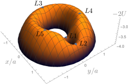
Figure 1: A three-dimensional representation of the effective binary potential in the co-rotating frame for a binary with mass ratio $q=0.1$. Here we have plotted twice the Roche potential, $-2U$, the negative of the Jacobi constant for a particle with zero velocity (see Eq. 1). The x and y coordinates in the binary plane are measured in units of the binary separation $a$. The primary and secondary are located at $(x_{p},y_{p})=(-a/(1+1/q),0)$ and $(x_{s},y_{s})=(a/(1+q),0)$ respectively. The five Lagrange points are labeled for reference.

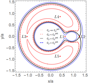
Figure 2: Zero-velocity curves for four different values of the Jacobi constant for a binary with mass ratio $q=M_{s}/M_{p}=0.1$ (level curves of the potential plotted in Figure 1). For $C_{J}\geq C^{\rm{crit}}$ (blue thick dashed and solid black), the zero-velocity curves connect, separating the binary plane into distinct inner and outer regions (as well as a third region around the secondary for large enough values of the Jacobi Constant). For $C_{J}<C^{\rm{crit}}$ (red lines), the zero-velocity curves open at L2 and then at L3 for even smaller $C_{J}$. The critical zero-velocity curve (black) passes through the Lagrange point L2. The five Lagrange points are labeled for reference.

To determine the structure of the R3B disc, we ask if particles in the inner disc have $C_{J}<C^{\rm{crit}}_{J}$; if so, they may be evacuated by the binary to form a central cavity. If the majority of particles in the inner (outer) disc have $C_{J}>C^{\rm{crit}}_{J}$, then they are trapped in the inner (outer) disc, and an annular gap will define the density structure. This analysis does not determine whether the un-trapped orbits actually cross the ZVCs or not - this depends on the initial magnitude and orientation of the velocity vector of each particle that is not trapped by the critical ZVC (green regions of Figure 3 below). We determine the fate of the un-trapped particles in §2.2.

Since the value of $C_{J}$ depends on a particle’s position as well as its velocity, we must prescribe a velocity profile in the disc. We choose a prescription given by the virial theorem which approaches the Keplerian value for the binary at large $r\equiv\sqrt{x^{2}+y^{2}}$ and the Keplerian value for each BH at $r\rightarrow r_{p}$ and $r\rightarrow r_{s}$

$$v_{\phi}=\sqrt{\frac{GM_{s}}{r_{s}}+\frac{GM_{p}}{r_{p}}}-r\Omega_{\rm{bin}}.$$ (2)

where $r_{p}$ and $r_{s}$ are the $\phi$ dependent distances from the primary and secondary, and we subtract the angular frequency $\Omega_{\rm{bin}}$ because we are working in the rotating frame of the binary.

Given the velocity profile in Eq. (2), Figure 3 displays the morphology of restricted regions in the binary orbital plane. Particles trapped in the outer (inner) disc have Jacobi constant greater than the critical value and are painted blue (red). Disc particles which are not restricted to either region are painted green. The enclosed area of the critical ZVC, which also consists of un-trapped particles, is painted dark-green.

We emphasize that the shape of the restricted regions depends on the choice of velocity profile, while the ZVCs are independent of this choice. An extreme choice of $|v|=0$ in the co-rotating frame causes the blue and red regions to extend to the boundary of the dark green region; all particles outside of the critical ZVC are forbidden to cross into the area enclosed by the ZVC. Conversely, if the velocities in the co-rotating frame are large, the red region can vanish and the blue region can recede far from the binary. This, however, is just a result of filling the system with initially unbound particles and has little meaning for an accretion disc. Choosing a purely Keplerian velocity distribution can also cause issues. The Keplerian velocity approaches infinity at the origin regardless of primary position. The result is an artificial depletion of trapped inner-disc particles for larger mass ratios. Thus, to create a representation that realistically describes the restricted regions in a quasi-steady-state CBD, one must choose a velocity distribution near an equilibrium state (though one may not exist for larger mass ratios) and without artificial singularities. This leads us to Eq. (2).

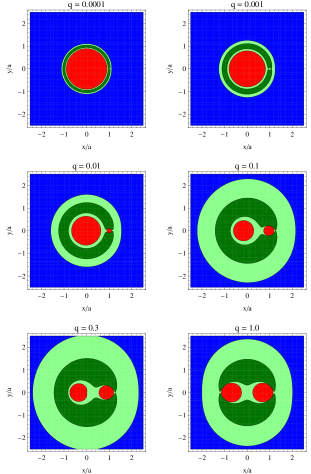
Figure 3: The dark green regions are bounded by the zero-velocity curve which passes through L2, delineating the smallest restricted regions which connect and separating the binary plane into distinct inner and outer regions. Particles trapped outside (inside) of the dark green region are labeled blue (red). Depending on their velocity vectors, light- and dark-green particles are free to move from inner to outer regions.

Because the green regions in Figure 3 consists of particles which are free to cross the binary orbit, we identify these regions with a putative gap/cavity. We examine this claim in §2.2 and find that their locations provide an adequate tracer for the gap/cavity size and shape. Furthermore, the locations of the outer gap/cavity edge identified in this manner, and those found in Figure 5 below, agree with the locations of circumbinary disc truncation computed from the stability and intersection of periodic R3Bp orbits (Rudak & Paczynski, 1981). This suggests a correspondence between locations in the outer binary potential where periodic orbits exist, and locations where particles with approximately Keplerian velocity are trapped outside the binary orbital barrier.

We note that the meaning of our Jacobi constant analysis in regions where periodic orbits cannot exist is somewhat ambiguous. In these regions, we must assign velocities to particles which do not correspond to fluid velocities in a stable disc. Rudak & Paczynski (1981) have delineated these regions explicitly, and they turn out to coincide with the green, untrapped particles of our analysis. As long as this is true, our analysis is consistent with particle stability considerations.

As the binary mass ratio is increased, Figure 3 shows that the putative gap grows in size and also morphs in shape from a small horseshoe, or annulus, in the orbit of the secondary, to a cavernous shape which includes the inner region. Additionally, as the mass ratio is increased, the fraction of particles trapped in a disc around the primary decreases while the number of particles trapped in a disc around the secondary increases. The following picture appears: for small mass ratios, the system consists of an inner disc (red) and outer disc (blue) separated by a low-density annulus. For larger mass ratios, Figure 3 depicts circum-primary and circum-secondary (mini-)discs (red) surrounded by a CBD (blue). The change in disc morphology is the most stark between the $q=0.01$ and $q=0.1$ panels of Figure 3.

Within the analysis so far, the transition between an inner and outer disc, vs. mini-discs+CBD, is defined only by terminology. There is however an important dynamical transition which occurs within the R3Bp for mass ratios $q>0.04$, namely the loss of stable orbits around the L4/L5 equilibrium points in the binary co-orbital region. In what follows we provide evidence for a well-defined and physically meaningful critical mass ratio, related to this stability criterion, which divides the two regimes described above.

2.2 Restrictions on Orbits from Equations of Motion

We now elaborate on the picture painted in Figure 3 by integrating the circular R3Bp equations of motion for a disc of $256^{2}$ test particles with initial velocity given by Eq. (2). We paint each of the particles the colour corresponding to its initial location in Figure 3. Using an adaptive step, Dormand Prince, 5th order Runge Kutta method (Press et al., 2007), we evolve the orbit of each particle for 100 binary orbits, conserving the Jacobi Constant to fractional order better than $10^{-6}$ (the majority of orbits conserve $C_{J}$ to machine precision). Note that, for large-mass-ratio binaries, a small fraction of the green particle orbits conserve $C_{J}$ to only the $10^{-2}$ level. This occurs for green particles which undergo large accelerations and move to large distances early in the evolution and does not affect the fate of the disc.

Figure 4 shows the location of each particle after only one binary orbit. During the first binary orbit, for mass ratios $q\mathrel{\hbox to0.0pt{\lower 4.0pt\hbox{\hskip 1.0pt$\sim$}\hss}\raise 1.0pt\hbox{$>$}}0.04$, the green regions funnel towards the L2 and L3 points into streams reminiscent of those seen in hydrodynamical simulations and also in the R3Bp study of D’Orazio et al. (2013). Recall that the green particles have Jacobi Constant corresponding to ZVCs which are not connected, but which still delineate a restricted region (red-dashed curve in Figure 2). The ZVCs of the green particles allow transfer of the green particles between inner and outer disc via the lowest barriers in the Roche potential, the L2 and L3 points respectively (the lowest point in the potential, L1, allows transfer between primary and secondary - see Figures 1 and 2). Without additional forces due to viscosity, pressure, or particle self gravity, the streams do not persist after a few orbits. If, however, dissipative forces refill the green region, or particles can interact, the streams continue to form as is seen in hydrodynamical simulations (see Figure 16 of the Appendix).

For smaller mass ratios $q\mathrel{\hbox to0.0pt{\lower 4.0pt\hbox{\hskip 1.0pt$\sim$}\hss}\raise 1.0pt\hbox{$<$}}0.04$, the L3 equilibrium point is much higher than the L2 point and particles stream in horseshoe orbits past L2 only. The particle density structure, in the $q=0.0001$ and $q=0.001$ cases (Figure 4), is reminiscent of low-mass-ratio hydrodynamical simulations where a spiral density wave propagates from the location of the secondary (see the top left panel of Figure 9 below).

Figure 5 shows the final location of each particle, after 100 binary orbits. We find that the red and blue particles do indeed remain trapped on their respective sides of the binary orbit. For $q\leq 0.001$ the green particles move along horseshoe and tadpole (horse-pole) orbits. As we approach $q=0.01$, we find green particles librating around the L4 or L5 points. Figure 6 zooms in on mass ratios between $q=0.02$ and $q=0.08$; for $q\mathrel{\hbox to0.0pt{\lower 4.0pt\hbox{\hskip 1.0pt$\sim$}\hss}\raise 1.0pt\hbox{$<$}}0.04$, some green particles remain in the co-orbital region. For mass ratios $q\mathrel{\hbox to0.0pt{\lower 4.0pt\hbox{\hskip 1.0pt$\sim$}\hss}\raise 1.0pt\hbox{$>$}}0.04$, green particles are cleared from the binary orbit. This is due to the lack of stable L4/L5 orbits in the R3Bp for $q>0.04$. The widening of the annulus and loss of particles on horse-pole orbits at $q\simeq 0.04$ marks a dynamically significant transition caused by a change in orbital stability. This loss of orbital stability will be especially important in the hydrodynamical case, where particles can interact.

$\begin{array}[]{c c }\includegraphics[scale={0.38}]{q0p0001_ecc0_norb1_Vprof4_Np256_r2p5_Rk5AdptStep}&\includegraphics[scale={0.38}]{q0p001_ecc0_norb1_Vprof4_Np256_r2p5_Rk5AdptStep}\\ \includegraphics[scale={0.38}]{q0p01_ecc0_norb1_Vprof4_Np256_r2p5_Rk5AdptStep}&\includegraphics[scale={0.38}]{q0p1_ecc0_norb1_Vprof4_Np256_r2p5_Rk5AdptStep}\\ \includegraphics[scale={0.38}]{q0p3_ecc0_norb1_Vprof4_Np256_r2p5_Rk5AdptStep}&\includegraphics[scale={0.38}]{q1_ecc0_norb1_Vprof4_Np256_r2p5_Rk5AdptStep}\end{array}$

Figure 4: Each panel is the result of evolving an initially spatially random distribution of particles, within radius $r<2.5a$, via the R3Bp equations, for one binary orbital period. The colouring of particles refers to the initial placement of a particle as in Figure 3. The black diamonds mark the Lagrange points (see Figures 1 and 2). These snapshots, after only one binary orbit, show the formation of streams acting to deplete green particles.

$\begin{array}[]{c c }\includegraphics[scale={0.38}]{q0p0001_ecc0_norb100_Vprof4_Np256_r2p5_Rk5AdptStep}&\includegraphics[scale={0.38}]{q0p001_ecc0_norb100_Vprof4_Np256_r2p5_Rk5AdptStep}\\ \includegraphics[scale={0.38}]{q0p01_ecc0_norb100_Vprof4_Np256_r2p5_Rk5AdptStep}&\includegraphics[scale={0.38}]{q0p1_ecc0_norb100_Vprof4_Np256_r2p5_Rk5AdptStep}\\ \includegraphics[scale={0.38}]{q0p3_ecc0_norb100_Vprof4_Np256_r2p5_Rk5AdptStep}&\includegraphics[scale={0.38}]{q1_ecc0_norb100_Vprof4_Np256_r2p5_Rk5AdptStep}\end{array}$

Figure 5: Same as Figure 4 except after 100 binary orbital periods.

$\begin{array}[]{c c}\includegraphics[scale={0.38}]{q0p02_ecc0_norb100_Vprof4_Np256_r2p5_Rk5AdptStep}&\includegraphics[scale={0.38}]{q0p04_ecc0_norb100_Vprof4_Np256_r2p5_Rk5AdptStep}\\ \includegraphics[scale={0.38}]{q0p06_ecc0_norb100_Vprof4_Np256_r2p5_Rk5AdptStep}&\includegraphics[scale={0.38}]{q0p08_ecc0_norb100_Vprof4_Np256_r2p5_Rk5AdptStep}\end{array}$

Figure 6: The same as Figure 5 except zooming in on the mass-ratio range $0.02\leq q\leq 0.08$.

2.3 Hydrodynamical Effects

Before numerically solving the viscous hydrodynamical equations, we attempt to estimate the effects of pressure and viscosity by making simple extensions to the standard R3Bp. Pressure and viscosity provide additional forces in the R3Bp equations of motion which destroy the conservation of $C_{J}$ and modify orbital stability in the standard R3Bp.

2.3.1 Pressure

Hydrodynamic pressure can be thought of as altering the effective potential of the binary at any point along a particle’s trajectory thus altering the ZVCs and hence the boundaries of the restricted regions in the previous section. We estimate the magnitude of pressure below which the R3B analysis may still be relevant by comparing the Jacobi constant to the analogue for a pressurized flow, Bernoulli’s constant

$$C_{B}=2U-v^{2}-2\int{\frac{dP}{\rho}},$$ (3)

where the integral is along the trajectory of a fluid element from a reference point to the point of evaluation. Subtracting Eqs. (1) and (3) we find $2\int{dP/\rho}=C_{J}-C_{B}$. By setting the difference in integrals of motion equal to the change in Jacobi constant across the binary orbit, we estimate the level of disc pressure necessary to overflow the previously described restricted regions of the purely gravitational problem (see Paczynski & Rudak, 1980; Rudak & Paczynski, 1981, who perform a similar calculation). For an ideal gas,

$$\int{\frac{dP}{\rho}}=\frac{(c^{\rm{ad}}_{s})^{2}}{\gamma-1}=\frac{\gamma(c^{\rm{iso}}_{s})^{2}}{\gamma-1}\quad\rm{Adiabatic}\ \rm{Flow}$$

$$\int{\frac{dP}{\rho}}=(c^{\rm{iso}}_{s})^{2}\ln{\frac{\rho}{\rho_{0}}}\quad\rm{Isothermal}\ \rm{Flow},$$ (4)

where the isothermal sound speed $c^{\rm{iso}}_{s}$ is related to the adiabatic sound speed $c^{\rm{ad}}_{s}$ by a factor of the adiabatic index $\gamma$. In the last line, the ratio $\rho/\rho_{0}$ comes from integrating from reference position outside of the binary orbit at density $\rho_{0}$, to a point inside the putative gap/cavity at density $\rho$.

The condition for vertical hydrostatic equilibrium in a thin Keplerian disc is $P/\rho=(GM/r)(H/r)^{2}$. This allows us to write the sound speed $\gamma(c^{\rm{iso}}_{s})^{2}=(c^{\rm{ad}}_{s})^{2}=\gamma\Omega^{2}_{K}H^{2}$ in terms of the Keplerian angular frequency of the disc $\Omega_{K}$ and disc height $H$. Then the disc orbital Mach number can be expressed as $\mathcal{M}\equiv v_{k}/c^{\rm{iso}}_{s}=(H/r)^{-1}$, encoding the temperature and pressure forces for a disc in vertical hydrostatic equilibrium. From vertical hydrostatic balance, we place a condition on the disc aspect ratio, at the location of the secondary, for which pressure forces can overcome the binary gravitational barrier,

$$\left(\frac{H}{r_{s}}\right)^{-1}_{\rm{ad}}\mathrel{\hbox to0.0pt{\lower 4.0pt\hbox{\hskip 1.0pt$\sim$}\hss}\raise 1.0pt\hbox{$<$}}\sqrt{2\frac{\gamma}{\gamma-1}\frac{GM_{\rm{bin}}}{\Delta C^{\rm{gap}}_{J}a}(1+q)}$$

$$\left(\frac{H}{r_{s}}\right)^{-1}_{\rm{iso}}\mathrel{\hbox to0.0pt{\lower 4.0pt\hbox{\hskip 1.0pt$\sim$}\hss}\raise 1.0pt\hbox{$<$}}\sqrt{2\left|\ln{\left(\frac{\rho}{\rho_{0}}\right)}\right|\frac{GM_{\rm{bin}}}{\Delta C^{\rm{gap}}_{J}a}(1+q)},$$ (5)

where $\Delta C^{\rm{gap}}$ is the variation of $C_{J}$ across the dark-green restricted regions of Figure 3. Operationally, we choose $\Delta C^{\rm{gap}}$ to be the difference in $C_{J}$ at L2 and L4 (or L5), as this is the largest $\Delta C$ spanning the dark-green restricted regions.

We emphasize that Eqs. (5) are not gap/cavity closing conditions; they are necessary conditions for the pressure to overcome the gravitational barrier of the binary. These conditions do not take into account the direction of pressure forces, and they do not consider hydrodynamical shocks, which have been shown, in the small mass ratio regime ($q\leq 10^{-3}$), to be responsible for gap opening in competition with viscous forces (Dong et al., 2011a; Dong et al., 2011b; Duffell & MacFadyen, 2013; Fung et al., 2014; Duffell, 2015). True gap/cavity closing conditions must incorporate a full hydrodynamical treatment, whereas the conditions (5) provide a necessary condition for pressure to dominate the flow dynamics.

In Figure 7 we plot critical disc aspect ratios (5) as a function of binary mass ratio. Over-plotted dots mark the positions of hydrodynamical simulations run in this study (§3). For the density ratio $\rho/\rho_{0}$ across a gap/cavity, we use the empirical relation from Duffell & MacFadyen (2013). All of the primary simulations run in this study have disc aspect ratios below the critical limit. To probe this limit we run high aspect ratio, $q=1$ hydrodynamical simulations for the isothermal and adiabatic cases (see §3). Figure 8 shows that the results of these high-aspect-ratio (equivalently, high pressure, thick disc, high temperature, or low-orbital-Mach number) simulations are in agreement with our Eqs. (5). The isothermal case shows a stark difference between an overflowed cavity at $H/r_{s}=1/3$ and a cleared cavity at $H/r_{s}=1/6$ while the adiabatic case is less extreme, with the $\mathcal{M}=3$ adiabatic case exhibiting a marginal central cavity.

Duffell & MacFadyen (2013) have shown that in the small mass ratio, thin disc case, the clearing of a gap always occurs for inviscid discs. This is because, in the absence of viscous forces, density waves generated by the binary will shock and deposit angular momentum into the disc clearing a gap without competition. It is not clear wether this is always true for high mass ratio, highly-pressurized discs; the overflowed CBDs in Figure 8 may eventually clear a cavity due to shocks, overcoming pressure on a longer timescale than considered here.

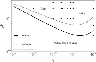
Figure 7: Delineation of different phases in a non-viscous circumbinary disc. The y-axis records the inverse disc aspect ratio, equivalent to the orbital Mach number; a smaller value signifies larger pressure forces; large pressure forces preclude reasoning based on a purely gravitational analysis. Points represent the parameters of hydrodynamical simulations run in this study (§3). Red denotes a simulation with a filled gap/cavity.

In summary, a necessary condition for pressure forces to overflow the binary cavity is predicted by Eq. (5). Equal-mass binary simulations show this condition to be sufficient in the large mass ratio regime, at least initially. Hence, having a high pressure in the disc does not impede the cavity formation, or whether it is lopsided, unless the pressure becomes so large that the disc is no longer thin. In this case, 3D effects can also become important, invalidating the 2D analysis above.

$\begin{array}[]{cc}\includegraphics[scale={0.24}]{ISO_rmx100_Dens2D_Norb1000_q1_alpha9e-06_Mach3}&\includegraphics[scale={0.24}]{ISO_rmx100_Dens2D_Norb01000_q1_alpha3p6e-05_Mach6}\\ \includegraphics[scale={0.24}]{ADI_rmx100_Dens2D_Norb1000_q1_alpha9e-06_Mach3}&\includegraphics[scale={0.24}]{ADI_rmx100_Dens2D_Norb1000_q1_alpha3p6e-05_Mach6}\vspace{-10 pt}\end{array}$

Figure 8: Snapshots of the surface density distribution (shown in units of the unperturbed value, with a logarithmic colour scheme) for an equal mass binary with disc aspect ratios ($r_{s}/H\equiv\mathcal{M}$) surrounding the pressure dominated condition Eq. (5). Here we set the viscosity to be very small (the coefficient of kinematic viscosity is $\nu=10^{-6}a^{2}_{0}\Omega_{\rm{bin}}$, where $\Omega_{\rm{bin}}$ is the binary angular frequency) in order to examine the analytic R3Bp prediction (5). The top row is for an isothermal equation of state $P=(c^{\mbox{iso}}_{s})^{2}\Sigma$ and the bottom row is for an adiabatic equation of state $P=(c^{\mbox{ad}}_{s})^{2}\Sigma^{5/3}$.

2.3.2 Viscosity

In order to more closely compare to viscous hydrodynamical simulations, and with the goal of linking orbital stability to the CBD phase transition, we follow Murray (1994) and Murray & Dermott (1999) to add an external viscous force $\mathbf{F}(x,y,\dot{x},\dot{y})$ to the R3Bp equations of motion. With these viscous R3Bp equations, we conduct a linear-stability analysis and integrate the viscous R3Bp equations of motion for a disc of test particles. We refer the interested reader to the Appendix for details; here we only state a brief summary of the three main conclusions.

1. Upon integrating the viscous R3Bp equations for an initial disc of test particles, we find that viscosity indeed acts to overflow gaps in the R3Bp and continually generates streams which penetrate the binary orbit (compare Figure 16 to Figure 5). The time rate of change of the Jacobi constant due to viscosity is given for a simple Keplerian velocity prescription in the Appendix.

2. The addition of viscosity causes orbits around L4 and L5 to become formally unstable for all binary mass ratios (Figure 14). However, the instability timescale for orbits below $q=0.04$ is of order a viscous time, while for $q>0.04$ it drops to of order the binary orbital time. Hence, viscosity does not greatly change the mass ratio at which orbits around L4 and L5 become effectively unstable. If the phase transition at $q=0.04$ is linked to the instability of orbits in the co-orbital region of the binary, then the level of viscosity should not greatly affect the mass ratio of the $q=0.04$ phase transition - for thin discs for which Eqs. (5) hold. We verify this with a suite of hydrodynamical simulations in the next section.

3. Viscosity induces a difference in orbital instability timescales for particle orbits around the L4 and L5 points (Figure 15). This difference is proportional to the magnitude of viscosity and it is small for $q<0.04$, becoming larger for $q>0.04$. While this asymmetry between L4 and L5 may aid in seeding the instability to an asymmetric cavity, it cannot be the only mechanism which causes the cavity to be lopsided. For example, symmetry between L4 and L5 must be restored at $q=1$, and a prominent asymmetry still appears in the disc morphology in this case. Future work will explore in more detail the relationship between the different orbital stability timescales and the cavity morphology.

3 Hydrodynamical simulations

3.1 Fiducial Simulations

In this section we show that the intuition gained from the R3Bp carries over to the hydrodynamical regime by running viscous 2D hydrodynamical simulations of the binary-disc system. We utilize the moving mesh code DISCO (Duffell & MacFadyen, 2011) to simulate a binary embedded in a locally isothermal, initially uniform surface density ($\Sigma=\rm{cst.}$) disc. To enforce a locally isothermal equation of state, the vertically integrated pressure is set as $P=(v_{\rm{eff}}/\mathcal{M})^{2}\Sigma$, where

$$v_{\rm{eff}}=\sqrt{\frac{GM_{s}}{r_{s}}+\frac{GM_{p}}{r_{p}}}$$ (6)

is the initial azimuthal velocity in the disc for an initially, spatially constant Mach number $\mathcal{M}$, and $\Sigma$ is the disc surface density. The initial radial velocity is given by viscous diffusion

$$v_{r}=-\frac{3}{\Sigma r^{1/2}}\partial_{r}\left[\nu\Sigma r^{1/2}\right],$$ (7)

where we choose a coefficient of kinematic viscosity which is constant in space and time $\nu=\alpha a^{2}_{0}\Omega_{0}/\mathcal{M}^{2}$, for fiducial values $\alpha=0.01$ and $\mathcal{M}=20$. These choices assure gap/cavity formation for $q\mathrel{\hbox to0.0pt{\lower 4.0pt\hbox{\hskip 1.0pt$\sim$}\hss}\raise 1.0pt\hbox{$>$}}10^{-4}$. Here $a_{0}$ and $\Omega_{0}$ represent the fixed separation and angular frequency of the binary. The simulation domain extends from the origin to $r_{\rm{max}}=12.0a$ employing a log grid ($r_{\rm{max}}$ can range from $8.0a$ to $100.0a$ for non-fiducial disc parameters as discussed in §3.2). The radial resolution is $\Delta r\sim 0.02a$ inside the binary orbit, similar to that of Farris et al. (2014), except we do not add an additional high-resolution region around each BH. We choose an outflow outer boundary condition. We do not apply an inner boundary condition and instead allow gas to flow through six cells at $r<0.05a$. Around each binary component we employ a density sink of size $r_{\rm{acc}}$ which removes gas at the rate $3/2\Sigma r^{-2}_{n}\nu$ from each cell within the sink radius, where $r_{n}$ is the distance from the $n^{\rm{th}}$ binary component. The total accretion rate onto each binary component is found by integrating over each cell located inside of the sink radius. Unless otherwise specified, we set $r_{\rm{acc}}=\rm{min}\left\{R_{\rm{Hill}},0.5a\right\}$ for the secondary and $r_{\rm{acc}}=0.5a$ for the primary, where $R_{\rm{Hill}}$ is the Hill radius of the secondary.

We evolve the viscous hydrodynamical equations for at least one viscous time at the location of the binary. We plot the resulting 2D surface-density distribution for different mass ratios in Figure 9. We make three observations on the CBD-density structure:

• An annular gap morphs into a central cavity: Comparing the $q=0.03$ and the $q=0.05$ panels in Figure 9, we see that there is a transition occurring by $q=0.03$ from an annular gap to a lopsided cavity (consistent with Farris et al. (2014) which used a hotter and more viscous disc) as well as a constant $\alpha$ (as opposed to constant $\nu$) viscosity prescription. We explore the dependence of the critical mass ratio on disc Mach number and viscosity in §3.2 below.

• The surface density decreases in the co-orbital region: The surface density in the annular gap decreases with increasing mass ratio until the gap becomes nearly devoid of gas above the transition to a lopsided cavity. While there are multiple factors that determine gap depth (and width; Fung et al., 2014; Kanagawa et al., 2015; Duffell, 2015), we note that the loss of stable orbits librating around L4/L5 and the disappearance of gas near the orbit of the secondary occur near the same mass ratio, suggesting that the existence of stable L4/L5 orbits may be necessary for long-lived gas in the gap. This behaviour helps to define the phase transition occurring at the same mass ratio.

• A lopsided, precessing cavity appears: The hydrodynamical study introduces a phenomenon accompanying the annular-gap to central-cavity transition which is not captured by the R3Bp alone, a lopsided, precessing cavity. This is illustrated by the surface density contours in the bottom panels of Figure 9. A lopsided cavity has been observed in previous studies which have used different numerical codes and physical assumptions (MacFadyen & Milosavljević, 2008; Shi et al., 2012; Noble et al., 2012; D’Orazio et al., 2013; Farris et al., 2014, 2015a, 2015b; Dunhill et al., 2015; Shi & Krolik, 2015). A complete description of the growth of lopsided cavities, especially in the symmetric equal-mass binary case, does not yet exist. However, the growth has been attributed to an initially small asymmetry in stream generation which causes a feedback loop between stream strength and cavity-edge location (Shi et al., 2012; D’Orazio et al., 2013). We observe that lopsided cavities are generated when stable orbits do not exist in the co-orbital region. Hence, the generation of a lopsided cavity may be intimately tied to orbital dynamics in the co-orbital region. When there are no stable co-orbital orbits, fluid passing into the co-orbital regime is flung into the outer disc rather than librating on stable orbits.

$\begin{array}[]{c c c}\includegraphics[scale={0.31}]{Dens2D_Norb5000_q0p001_alpha0p01_Mach20}&\includegraphics[scale={0.31}]{Dens2D_Norb5000_q0p01_alpha0p01_Mach20}&\includegraphics[scale={0.31}]{Dens2D_Norb5000_q0p03_alpha0p01_Mach20}\\ \includegraphics[scale={0.31}]{Dens2D_Norb5000_q0p05_alpha0p01_Mach20}&\includegraphics[scale={0.31}]{Dens2D_Norb5000_q0p1_alpha0p01_Mach20}&\includegraphics[scale={0.31}]{Dens2D_Norb5000_q1_alpha0p01_Mach20}\end{array}$

Figure 9: Snapshots of the surface density distribution (shown in units of the unperturbed value, with a logarithmic colour scheme) from hydrodynamical simulations for a disc with orbital Mach number $\mathcal{M}\equiv r/H\equiv v_{\rm{eff}}/c_{s}=20$, and constant coefficient of kinematic viscosity $\nu=0.01a^{2}_{0}\Omega_{\rm{bin}}/\mathcal{M}^{2}$. The binary mass ratio increases from left to right, top to bottom, as labeled. For small mass ratios, the system is in nearly steady-state and an annular gap is cleared in the orbit of the secondary black hole. For $q\mathrel{\hbox to0.0pt{\lower 4.0pt\hbox{\hskip 1.0pt$\sim$}\hss}\raise 1.0pt\hbox{$>$}}0.03$, the gap morphs into an even lower density time-dependent, precessing central cavity. The critical zero-velocity curve, which passes through L2, is over-drawn in white. The relatively shallow annular gap in the $q=0.001$ case is difficult to see on this scale because the accretion prescription and inner boundary cause the inner disc to drain onto the primary.

To further examine the connection between orbital stability and the transition to a time-dependent, lopsided cavity, we track the flow of gas in the co-orbital region. To do this we evolve separate conservation equations for two passive scalars. A passive scalar is a scalar quantity which obeys a conservation equation given an initial concentration and the fluid velocities from the hydrodynamic problem. We start one scalar outside of the critical ZVC and the other inside. The light green regions of Figures 3 and 5 show that, even in the non-hydrodynamic case, this setup should result in the passive scalars moving across the orbit of the binary, which is what we wish to track. Figure 10 plots the evolution of the passive scalars as well as fluid-velocity vectors for three different mass ratios. We colour the passive scalar which is initially inside (outside) of the critical ZVC red (blue).

$\begin{array}[]{cccc}\includegraphics[scale={0.3}]{1Panel_AllLpoints_PScalDens_ZVCInOut_Norb0001p00_q0p001.png}&\includegraphics[scale={0.3}]{1Panel_AllLpoints_PScalDens_ZVCInOut_Norb0002p00_q0p001.png}&\includegraphics[scale={0.3}]{1Panel_AllLpoints_PScalDens_ZVCInOut_Norb0004p00_q0p001.png}&\includegraphics[scale={0.3}]{1Panel_AllLpoints_PScalDens_ZVCInOut_Norb0008p00_q0p001.png}\\ \includegraphics[scale={0.3}]{1Panel_AllLpoints_PScalDens_ZVCInOut_Norb0001p00_q0p01}&\includegraphics[scale={0.3}]{1Panel_AllLpoints_PScalDens_ZVCInOut_Norb0002p00_q0p01}&\includegraphics[scale={0.3}]{1Panel_AllLpoints_PScalDens_ZVCInOut_Norb0004p00_q0p01}&\includegraphics[scale={0.3}]{1Panel_AllLpoints_PScalDens_ZVCInOut_Norb0008p00_q0p01}\\ \includegraphics[scale={0.3}]{1Panel_AllLpoints_PScalDens_ZVCInOut_Norb0001p00_q0p05}&\includegraphics[scale={0.3}]{1Panel_AllLpoints_PScalDens_ZVCInOut_Norb0002p00_q0p05}&\includegraphics[scale={0.3}]{1Panel_AllLpoints_PScalDens_ZVCInOut_Norb0004p00_q0p05}&\includegraphics[scale={0.3}]{1Panel_AllLpoints_PScalDens_ZVCInOut_Norb0008p00_q0p05}\end{array}$

Figure 10: Evolution of two passive scalars for $q=0.001$, $q=0.01$, and $q=0.05$ (rows) at different times (columns) during gap opening as well as velocity vectors showing fluid motion in the co-rotating frame. The red scalar starts inside of the critical ZVC (overlaid, black curve) and the blue scalar starts outside. The green dots denote the Lagrange points of the binary potential (See Figures 1 and 2). Published with this article are movies of the above three simulations with the red and blue passive scalars plotted on different panels and with the same initialization as Figure 3 (these movies and the corresponding movies of surface density evolution can also be found at http://user.astro.columbia.edu/$\sim$dorazio/moviespage).

The first row in Figure 10 tracks the fluid motion for a binary mass ratio well below the stability/phase transition, $q=0.001$. It is clear that gas inside the orbit moves outwards across the position of the secondary at L2 and travels along the horseshoe orbits delineated by the critical ZVC. Gas initially outside of the orbit similarly moves across L2 and enters onto horseshoe orbits which eventually deposit the gas onto the inner disc.

The second row in Figure 10 tracks the fluid motion for a binary with $q=0.01$, which is still below the R3Bp linear-stability mass ratio. From the velocity vectors it is clear that the mean motion of the fluid is along the horseshoe and librating L4/L5 orbits. In the $q=0.01$ case, the velocity of the fluid is larger in the presence of larger binary forces. The result is a greater deviation of the gas from the critical ZVC curve, some of which begins to peel off into the outer disc. As the last panel for the $q=0.01$ case hints, this behaviour is not sustained once the gap is cleared and a steady state ensues.

The third row in Figure 10 tracks the fluid motion for $q=0.05$, which is above the mass ratio for which stable L4/L5 orbits exist. We now see that the red gas immediately flows out along L3 and L2. The gas leaving L3 connects back to the orbital flow around L4 while the gas leaving L2 is flung into the disc. A striking feature is the large velocity vectors pointing outward from between L2 and L5 into the disc rather than pointing back along the horseshoe orbit. Because of the vigorous ejection of fluid from the L5 point, an asymmetry builds between the L4 and L5 regions.

In addition to the ejection of co-orbital particles for $q\mathrel{\hbox to0.0pt{\lower 4.0pt\hbox{\hskip 1.0pt$\sim$}\hss}\raise 1.0pt\hbox{$>$}}0.04$, we observe the beginnings of a second stream connecting to the primary through the L3 equilibrium point, the lowest point in the binary potential after L1 and L2. The bottom panels of Figure 9 show us that, for near equal mass binaries, two accretion streams feed the binary. Previous work (Shi et al., 2012; D’Orazio et al., 2013) has argued that streams crashing into the surrounding CBD causes lopsided cavity growth. Specifically, (D’Orazio et al., 2013) conducted an experiment where a disc around an equal mass binary is simulated with one binary component placed artificially at the origin of coordinates. In this experiment, only one stream is generated and lopsided growth is inhibited. Hence, though it may not be necessary for lopsided growth, the generation of a second, strong stream for $q\mathrel{\hbox to0.0pt{\lower 4.0pt\hbox{\hskip 1.0pt$\sim$}\hss}\raise 1.0pt\hbox{$>$}}0.04$ seems to facilitate such growth.

Because the new stream through L3 feeds the primary, the $q=0.04$ transition also signifies an increase in the accretion rate of the primary relative to the secondary for $q\mathrel{\hbox to0.0pt{\lower 4.0pt\hbox{\hskip 1.0pt$\sim$}\hss}\raise 1.0pt\hbox{$>$}}0.04$.

Finally, we note that, in order to show the dynamics of gap clearing, the flows depicted in Figure 10 are chosen at early times in the disc evolution. While initial conditions are chosen so that initial transients are minimal, such transients may be present, and one should take this example only as suggestive of the properties of the flow at later times.

3.2 Hydrodynamic Parameter Study

Although we identified a clear transition in the disc behaviour near $q=0.04$, it is natural to ask whether this critical value is universal, or if it depends on disc parameters. To determine this, we repeat our earlier hydrodynamical simulations but for two new values of the coefficient of kinematic viscosity $\nu_{0}=10^{-3}$, $10^{-4}$, where $\nu_{0}\equiv\nu a^{-2}_{0}\Omega^{-1}_{\rm{bin}}$, and two new values of the Mach number $\mathcal{M}=10$, $30$, corresponding to a factor of 9 variation in disc pressure and temperature. For each of the four new parings of Mach number and viscosity coefficient, we run four simulations at the binary mass ratios $q=0.01,0.025,0.075,0.1$.

Note that we increase the outer boundary of the simulation domain to $r_{\rm max}=16a$ for the $\nu_{0}=10^{-4}$, $\mathcal{M}=10$ simulation, because in these simulations, spiral density waves have longer wavelengths and are less damped by viscosity, allowing them to reach the outer boundary of the simulation, with the results therefore potentially depending on the outer boundary condition. For all other simulations we choose $r_{\rm max}=8a$. Because we are using a log grid, this corresponds to only a minimal change in resolution. We have run higher resolution simulations for the $\nu_{0}=10^{-4}$, $\mathcal{M}=10$ and $\nu_{0}=10^{-3}$, $\mathcal{M}=30$ cases with outer boundary at $r_{\rm max}=100a$ finding minimal changes in the surface density distributions, accretion rates, and disc lopsidedness presented below.

From our set of $8$ (fiducial) $+16$ (parameter study) $=24$ CBD simulations (Table 1), we use the following two diagnostics to track the onset of the $q\sim 0.04$ cavity transition.

1. Amplitude of accretion-rate variability: To emphasize the change from steady-state to strongly-fluctuating solutions across the CBD phase transition, we compute the standard deviation from the mean accretion rate measured separately onto the individual BHs, as well as the total accretion rate onto both BHs,

   $$\delta\dot{M}^{n} = \sqrt{\frac{1}{N-1}\sum^{N}_{j}\left(\dot{M}^{n}_{j}-\left<\dot{M^{n}}\right>_{t}\right)^{2}}$$

   $$\dot{M}^{n}(t) = \sum_{k}\frac{3}{2}\Sigma_{k}(t)(r^{n}_{k})^{-2}\nu\qquad k\mid r^{n}_{k}\leq r^{n}_{\rm acc}.$$ (8)

   In the top equation $j$ denotes the $j^{\rm th}$ timestep out of N total timesteps and $\left<\cdot\right>_{t}$ is the average over the entire time interval. In the bottom equation, $k$ denotes the $k^{\rm th}$ cell within the sink radius and the summation is over all cells within the sink radius. In both equations $n$ denotes the $n^{\rm th}$ binary component.

2. Disc Lopsidedness: To measure the lopsidedness of the cavity we measure the quantity

   $$\epsilon=\left<\left<\frac{\left|\left<\Sigma v_{r}\mbox{e}^{i\phi}\right>_{\phi}\right|}{\left<\Sigma v_{\phi}\right>_{\phi}}\right>_{r}\right>_{t},$$ (9)

   where $\left<\cdot\right>_{\phi}$ denotes an azimuthal average, $\left<\cdot\right>_{r}$ denotes a radial average from $r=a$ to the edge of the simulation domain, $\left<\cdot\right>_{t}$ denotes a time average over an integer number of binary orbits, and $|\cdot|$ is the magnitude of a complex number. The only non-zero contributions to Eq. (9) are from the components of $\Sigma v_{r}$ which are proportional to $A\cos{(\phi-\phi_{A})}+B\sin{(\phi-\phi_{B})}$, for arbitrary constants $A$, $B$, $\phi_{A}$, and $\phi_{B}$. Hence $\epsilon$ measures the lopsidedness of the disc. Note that $\epsilon$ is often referred to as the disc eccentricity (e.g., MacFadyen & Milosavljević, 2008; Farris et al., 2014).

The above diagnostics are time-averaged over the final 100 orbits of the simulation, for which a quasi-steady state has been achieved.

$q\equiv M_{s}/M_{p}$	$\mathcal{M}$	$\nu$
0.01, 0.025, 0.075, 0.1	10	$10^{-3}$
0.01, 0.025, 0.075, 0.1	10	$10^{-4}$
0.001, 0.01, 0.025, 0.03, 0.05, 0.075, 0.1, 1.0	20	$2.5\times 10^{-5}$
0.01, 0.025, 0.075, 0.1	30	$10^{-3}$
0.01, 0.025, 0.075, 0.1	30	$10^{-4}$

Table 1: Parameters for the simulations run in this study. The columns, from left to right, are the binary mass ratio, the orbital Mach number, and the coefficient of kinematic viscosity.

Figure 11 plots the accretion rate variability onto the secondary $\delta\dot{M}^{s}$ (left), primary $\delta\dot{M}^{p}$ (central), and both $\delta\dot{M}$ (right) BHs, as a function of binary mass ratio for each set of disc parameters. Because there is a scatter in the magnitude of accretion variability across the range of different disc parameters (notably, the magnitude of variability varies with viscosity), we normalize each set of mass ratios for a given set of disc parameters by the average $\delta\dot{M}$ over all $q$ (excluding the extreme values $q=0.001$ and $q=1$ for the fiducial case). First notice that the left and right panels of Figure 11, $\delta\dot{M}^{s}$ and $\delta\dot{M}$, are very similar. This is because over the range of mass ratios probed, the accretion rate onto the secondary, and any resulting variation, is larger than that onto the primary (in agreement with Farris et al. 2014). Both of these panels show a clear trend in increasing accretion variability across the $q=0.04$ transition, for all sets of disc parameters.

$\begin{array}[]{c c c}\includegraphics[scale={0.31}]{StdS_100.pdf}&\includegraphics[scale={0.31}]{StdP_100.pdf}&\includegraphics[scale={0.31}]{StdTot_100.pdf}\end{array}$

Figure 11: The standard deviation of $\dot{M}$ onto the secondary (left), primary (center), and both (right) BHs, computed over the final 100 orbits of each simulation. The vertical solid line is drawn at the $q=0.04$ transition, the dashed horizontal line is the mean of the standard deviation of each data set.

While observationally interesting, relative accretion rates measured onto the secondary (and hence the total accretion rate onto both black holes) may be a less robust diagnostic for the $q=0.04$ CBD transition than accretion rates measured onto the primary. The transition depicted by the central panel of Figure 11 - for the standard deviation of accretion rates onto the primary - looks sharper because the accretion rate variability settles down to small values below the $q=0.04$ transition. The same measurements, for accretion rate variability onto the secondary (and hence the total accretion rate variability), do not settle to as tight a range of small values. This effect may be tied to how accretion rates are measured in the simulation; for small mass ratios, accretion is measured in the small region within the Hill sphere of the secondary, and rates measured in the simulations may be sensitive to this sink size and the resolution. For example, for fiducial disc parameters, the $q=0.001$ and $q=0.025$ cases exhibit anomalously large variability onto the secondary, which is omitted from Figure 11. Future work should examine the dependence of accretion rates on sink size, accretion prescription, and resolution around the secondary. These considerations are, however, less important for the primary.

The central panel of Figure 11, displaying accretion variability onto the primary, exhibits the most striking depiction of the transition. This panel shows a sharp increase in variability amplitude across the $q=0.04$ transition for all disc parameters. An increased magnitude of accretion variability onto the primary is in agreement with the earlier observation that the stream feeding the primary BH becomes significant at the $q=0.04$ transition. Because the second stream could be necessary for generating the lopsided cavity, $\delta\dot{M}^{p}$ acts as an excellent diagnostic for the $q=0.04$ transition.

MacFadyen & Milosavljević (2008); Shi et al. (2012); Noble et al. (2012); D’Orazio et al. (2013); Farris et al. (2014, 2015a, 2015b); Shi & Krolik (2015) have shown that an equal-mass binary can create a lopsided CBD (referred to as eccentric in MacFadyen & Milosavljević (2008) and Farris et al. (2014)). Farris et al. (2014) measured the disc lopsidedness for a range of binary mass ratios, finding a sharp transition to lopsided discs for $q\mathrel{\hbox to0.0pt{\lower 4.0pt\hbox{\hskip 1.0pt$\sim$}\hss}\raise 1.0pt\hbox{$>$}}0.05$ (see Figures 5 and 6 of Farris et al. 2014). Figure 12 plots the time averaged disc lopsidedness, Eq. (9), measured at radii $r>a$, as a function of binary mass ratio. We find a sharp increase in disc lopsidedness near $q=0.04$ for all disc viscosities and pressures except for the high viscosity $\nu_{0}=10^{-3}$, low pressure case $\mathcal{M}=30$.

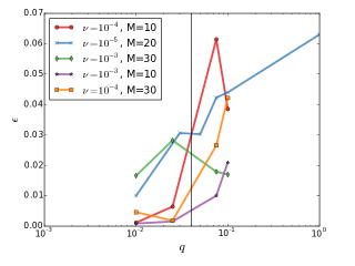
Figure 12: The lopsidedness, Eq. (9), of the circumbinary disc, spatially averaged over the region outside of the binary orbit, $r>a$, and time averaged over the final 100 orbits of each simulation. The vertical sold line denotes $q=0.04$.

We display the surface density of the $q=0.01$, $\nu_{0}=10^{-3}$, $\mathcal{M}=30$ disc in the left panel of Figure 13. In this case, strong shocks form intermittently as the spiral arm connecting to the secondary propagates outwards into the disc. These shocks lead to the formation of a slightly lopsided disc even for the $q=0.01$ case. We note that this asymmetry could be caused by the difference in instability times derived for the viscous R3Bp in the Appendix (see Figure 15). However, we leave an investigation for future work

$\begin{array}[]{c c}\includegraphics[scale={0.25}]{Dens2D_Norb0390_q0p01_alpha0p9_Mach30}&\includegraphics[scale={0.25}]{Dens2D_Norb0390_q0p1_alpha0p9_Mach30}\end{array}$

Figure 13: Snapshots of the surface density distribution (shown in units of the unperturbed value, with a logarithmic colour scheme) from hydrodynamical simulations for a disc with $\mathcal{M}=30$, and constant coefficient of kinematic viscosity $\nu=10^{-3}a^{2}_{0}\Omega_{\rm{bin}}$. For these high-viscosity, low-pressure simulations, we find an asymmetric-disc shape even for small mass ratio binaries (left). The transition to a time-dependent, lopsided cavity at $q\sim 0.04$ still takes over for larger mass ratio binaries (right).

In addition to the possible viscous instability explained in the Appendix, there are other mechanisms which may make the CBD lopsided and induce variable accretion. Kley & Dirksen (2006) find that a spatial gap asymmetry can be induced even for mass ratios as low as $q=0.003$. This is only found to occur when viscosity is low enough for a deep gap to be cleared. The explanation of Kley & Dirksen (2006) uses the work of Lubow (1991a, b); a deep gap mitigates the eccentric co-rotation resonances in the disc which act to damp disc lopsidedness while eccentric Linblad resonances (eLRs) act to grow disc lopsidedness. This asymmetry growth due to eLRs is not likely the mechanism causing the $q=0.04$ phase transition. Figures 11 and 12 show that the transition to a lopsided cavity occurs around $q=0.04$ even for large viscosities and that there is no trend of a decreasing critical mass ratio with decreasing viscosity as the Kley & Dirksen (2006) mechanism would predict. Additionally, Shi et al. (2012) show that the growth timescale of asymmetry for the $q=1$ binary does not match the growth timescale expected from the argument of Kley & Dirksen (2006). Future work should measure the growth rate of lopsidedness for multiple mass ratios in order to dis-entangle the mechanism by which the low mass ratio systems of Kley & Dirksen (2006) become asymmetric (presumably eLRs) and the mechanism which causes the phase transition studied here (presumably orbital instability).

Regardless of hydrodynamic processes which may act to grow a lopsided, time-variable disc below the $q=0.04$ transition, the present study shows that a robust transition in CBD structure dominates for $q\mathrel{\hbox to0.0pt{\lower 4.0pt\hbox{\hskip 1.0pt$\sim$}\hss}\raise 1.0pt\hbox{$>$}}0.04$ over a wide range of hydrodynamic disc parameters.

4 Discussion and Summary

Circumbinary accretion discs exhibit a phase transition above a binary mass ratio of $q\simeq 0.04$. The transition signifies a loss of spatial and time-translation symmetry in the CBD. The density structure changes from an annular low-density gap near the orbit of the secondary ($q\mathrel{\hbox to0.0pt{\lower 4.0pt\hbox{\hskip 1.0pt$\sim$}\hss}\raise 1.0pt\hbox{$<$}}0.04$), to a lopsided cavity ($q\mathrel{\hbox to0.0pt{\lower 4.0pt\hbox{\hskip 1.0pt$\sim$}\hss}\raise 1.0pt\hbox{$>$}}0.04$). It also marks a transition from steady-state to strongly-fluctuating behaviour. We conjecture that this transition is closely tied to the loss of stable orbits in the binary co-orbital region of the restricted three-body problem (R3Bp) for $q>0.04$. When stable co-orbital orbits connect the outer, circumbinary disc to the inner, circumprimary disc, steady-state gapped solutions are realized. When no such stable co-orbital orbits exist, accretion streams violently impact the inner mini-discs and the outer circumbinary disc, leading to fluctuating lopsided cavity solutions. We employ the R3Bp as well as 2D viscous hydrodynamical simulations to investigate the CBD transition.

We show that the change in density morphology, from annular gaps to cavities, in circumbinary accretion discs can be largely captured by the spatial restriction of test particles imposed by conservation of the Jacobi constant in the R3Bp. To quantify the limitations of the R3Bp and to more closely compare to hydrodynamical simulations, we extend the R3Bp analysis to include the effects of pressure and viscosity. To estimate the effects of pressure in the disc, we compare the Jacobi constant with the closely related Bernoulli constant and derive a maximum disc aspect ratio (minimum Mach number) necessary for pressure forces to overcome the gravitational barrier of the binary. For binaries with $q>0.04$ this only occurs for discs which are no longer thin.

To study the effects of viscosity on the R3Bp and investigate the relation of the CBD phase transition to orbit stability, we add a viscous force to the R3Bp equations and perform a linear-stability analysis on orbits around the L4 and L5 equilibrium points in the presence of this force. We find that the viscous R3Bp shares a similar orbital stability transition which occurs very near the classical stability mass ratio of $q=0.04$ over multiple magnitudes of viscosity (see the Appendix), consistent with our hydrodynamical parameter study. We also find that viscous forces break a symmetry between the stability of the leading and trailing triangular Lagrange points (L4/L5) of the classical R3Bp. This may be related to the growth of asymmetry in CBDs, though we save such a study for future work.

The effects of both viscosity and pressure on the CBD transition are studied via 2D viscous hydrodynamical simulations. These show that changing the disc viscosity by a factor of 40 and the disc pressure by a factor of 9 leaves the critical mass ratio largely unaffected. The hydrodynamical simulations also provides further evidence for a mechanism by which orbital instability seeds the transition. For $q\mathrel{\hbox to0.0pt{\lower 4.0pt\hbox{\hskip 1.0pt$\sim$}\hss}\raise 1.0pt\hbox{$<$}}0.04$ disc particles in the binary co-orbital region stably oscillate on horseshoe-like orbits, while for $q\mathrel{\hbox to0.0pt{\lower 4.0pt\hbox{\hskip 1.0pt$\sim$}\hss}\raise 1.0pt\hbox{$>$}}0.04$, particles are flung out of the co-orbital region into the outer disc (Figure 10).

We note that, in addition to loss of L4/L5 orbital stability, there is another dynamical transition which occurs near $q=0.04$ in the R3Bp. With the goal of determining the truncation of CBDs, Rudak & Paczynski (1981) studied the intersection and radial stability of test particle orbits around a circular binary with arbitrary mass ratio. They posit that the innermost stable orbits of a CBD are set either by orbit intersection, or instability to radial perturbations of a Keplerian orbit around the binary. They find that, for binaries with $q\mathrel{\hbox to0.0pt{\lower 4.0pt\hbox{\hskip 1.0pt$\sim$}\hss}\raise 1.0pt\hbox{$<$}}0.01$, orbit intersection truncates the CBD, for $0.01\leq q\leq 0.05$ the inner edge of the disc becomes marginally unstable before orbit intersection becomes important, and for $q>0.05$, violent instability is responsible for disc truncation. In this paper, we have shown evidence that links the L4/L5 orbital instability to the observed CBD transition. The additional radial instability found by Rudak & Paczynski (1981) in the particle limit, near the inner edge of the CBD, also occurs near q=0.05. However, our hydrodynamical simulations do not show strong fluctuations in the inner edge of the CBD for $q\mathrel{\hbox to0.0pt{\lower 4.0pt\hbox{\hskip 1.0pt$\sim$}\hss}\raise 1.0pt\hbox{$>$}}0.05$. Rather, the variability in the accretion rates we observe appears to track the unstable behavior of the gas near L4/L5 (see Figure 10 and corresponding movies).

In accordance with the simplicity of the circular R3Bp and our numerical simulations, we have restricted our analysis to systems consisting of isothermal and adiabatic thin discs surrounding a binary on a fixed circular orbit. A binary on an eccentric orbit exhibits loss of co-orbital stability at mass ratios smaller than $q=0.04$ of the circular case (Kovács, 2013). Supersonic gas dynamics in the vicinity of the binary will likely invalidate the assumption of an isothermal gas disc. A massive disc will move the binary; for mass ratios above the transition, the binary may become eccentric (Cuadra et al., 2009; Roedig et al., 2011, 2012) and migrate differently than the often assumed Type II rate (e.g. Haiman et al., 2009; Dotti et al., 2015). Future work should address the change of binary orbital parameters due to the change in CBD structure. Other important physics not included in this work may also impact the $q=0.04$ transition. Including the vertical disc dimension, magnetic fields and the magneto-rotational instability, and radiative feedback from accretion could all affect the onset and behaviour of the transition described here.

Future work on CBD structure may find insight into more general binary+disc systems from extensions of the circular R3Bp for a binary with time-dependent separation (Schnittman, 2010), a mis-aligned disc (Erwin & Sparke, 1999), or non-zero eccentricity (Pichardo et al., 2005).

Within the limitations of this study, we have identified a dramatic transition occurring in circumbinary discs and offered an intriguingly simple origin; further work should clarify whether it survives the additional physical effects mentioned above.

The $q=0.04$ CBD transition is relevant to MBHB+disc systems. Accreting MBHBs below the critical mass ratio will prove difficult to detect in time-domain electromagnetic surveys due to accretion variability alone. For such low mass, steadily-accreting MBHBs, other mechanism could cause variability, such as a precessing jet, disc instabilities, or relativistic Doppler boost in the case of compact binaries (D’Orazio et al., 2015b). Because of the drastic change in disc lopsidedness across the $q=0.04$ transition, there may be an equally drastic change in the binary orbital parameters. This would result in a connection of the binary mass ratio with binary eccentricity and migration rate. This could affect gravitational wave detection rates as well as waveforms.

The $q=0.04$ CBD transition is also relevant for proto-planetary systems. The formation of planets around a binary system may progress differently for a proto-planetary disc around a brown dwarf and main sequence pair (e.g, De Rosa et al., 2014; Curé et al., 2015; Hinkley et al., 2015) then for a near equal mass binary. Though theoretically disfavoured (Payne & Lodato, 2007), there would be important consequences for the formation of planetary systems around brown dwarfs which contain a large ($\mathrel{\hbox to0.0pt{\lower 4.0pt\hbox{\hskip 1.0pt$\sim$}\hss}\raise 1.0pt\hbox{$>$}}M_{J}$) planet. It will be interesting to look for differences in planetary populations around binaries above and below $q\sim 0.04$ if they are discovered in upcoming searches (e.g. Triaud et al., 2013; Ricker et al., 2014).

Appendix A Viscous, restricted three-body problem

We follow Murray (1994) and Murray & Dermott (1999) to add an external viscous force $\mathbf{F}(x,y,\dot{x},\dot{y})$ to the R3Bp equations of motion. In the rotating frame,

$$\begin{array}[]{c}\ddot{x}-2\Omega\dot{y}=\frac{\partial{U}}{\partial{x}}+F_{x}\\ \\ \ddot{y}+2\Omega\dot{x}=\frac{\partial{U}}{\partial{y}}+F_{y},\end{array}$$

where $\Omega$ is the frequency of the rotating frame and $U(x,y)$ is the Roche potential with sign convention taken to be consistent with Murray & Dermott (1999).

For the external force we use the force associated with the $r-\phi$ component of the viscous stress tensor in a Keplerian flow. In the inertial frame this force (per unit mass) is

$$\begin{array}[]{l}F_{\hat{\phi}}=\frac{\partial_{r}\sigma^{\hat{r}\hat{\phi}}}{\rho}=-\partial_{r}\left[\nu r\partial_{r}\Omega_{\rm disc}\right]=-\frac{9}{4}\nu\frac{v_{\phi}}{r^{2}},\end{array}$$

where we assume that the angular velocity of the flow is Keplerian around the binary mass $M$, and that the kinematic coefficient of viscosity $\nu$ and density $\rho$ are constants. In the last line we relabel $v_{\phi}\equiv\sqrt{GM/r}$ . By transforming to Cartesian coordinates and then moving into the rotating frame we find

$$\begin{array}[]{l}F_{x}=-F_{\hat{\phi}}\frac{y}{r}\\ \\ F_{y}=F_{\hat{\phi}}\frac{x}{r}.\end{array}$$

Writing these in terms of the rotating frame coordinates and velocities,

$$\begin{array}[]{l}F_{x}=-\frac{9}{4}\frac{\nu}{x^{2}+y^{2}}(\dot{x}-y\Omega)\\ \\ F_{y}=-\frac{9}{4}\frac{\nu}{x^{2}+y^{2}}(\dot{y}+x\Omega),\end{array}$$

which follows from our choice of azimuthal velocity profile $v_{\phi}(r)$ in the inertial frame of the binary so that $\dot{x}=-(v_{\phi}-r\Omega)y/r$ and $\dot{y}=(v_{\phi}-r\Omega)x/r$.

As with pressure forces (§2.3.1), viscous forces also destroy conservation of the Jacobi constant. $C_{J}$ changes at a rate

$$\dot{C_{J}}=\frac{9}{2}\frac{\nu}{x^{2}+y^{2}}\left[\dot{x}^{2}+\dot{y}^{2}+\Omega(x\dot{y}-y\dot{x})\right].$$ (10)

Comparing the change in $C_{J}$ due to viscosity to the change due to pressure over $N_{\rm orb}$ orbital times gives,

$$|\Delta C_{J}|_{\nu}=\alpha N_{\rm orb}\frac{5}{9\pi}|\Delta C_{J}|_{P},$$ (11)

where we have used Eq. (3) and the first of Eqs. (4) for the RHS and assumed a constant coefficient of kinematic viscosity $\nu=\alpha/\mathcal{M}^{2}a^{2}\Omega$ with $\alpha<1$. In the case that $N_{\rm orb}$ is a gap opening time, which we approximate as the viscous time across a gap of size equal to the disc scale height, we find

$$|\Delta C_{J}|_{\nu}=\frac{5}{27\pi^{2}}|\Delta C_{J}|_{P}\sim 0.02|\Delta C_{J}|_{P}.$$ (12)

Hence for short timescales relevant for local density distribution such as gaps, the pressure forces dominate in the decay of the Jacobi constant. For longer timescales $N_{\rm orb}\gg 1/\alpha$ it is viscosity which dominates the deviation from the purely gravitational problem.

To investigate the consequences of a viscous force for orbital stability, we perform a linear-stability analysis for particles perturbed from the analogue of the L4/L5 points in the viscous R3Bp (A), with external force (A). The location of the new equilibrium points in the presence of the viscous force are found by setting $\ddot{x}=\ddot{y}=\dot{x}=\dot{y}=0$ in the equations of motion (A) and solving for the coordinates $(x^{\dagger},y^{\dagger})$ of the new equilibrium points. Murray (1994) finds solutions by Taylor expanding the equations of motion around the $\mathbf{F}=0$ classical equilibrium points $(x_{0},y_{0})$ and solving for the deviation $(\bar{x},\bar{y})$ from $(x_{0},y_{0})$. To linear order in $\bar{x},\bar{y}$ the new equilibrium points are,

$$\begin{array}[]{l}x^{\dagger}=x_{0}-\frac{(1+q)}{q}\frac{F^{*}_{x}}{3}\pm\frac{(1+q)}{q}\frac{F^{*}_{y}}{3\sqrt{3}}\\ \\ y^{\dagger}=y_{0}\pm\frac{(1+q)}{q}\frac{F^{*}_{x}}{3\sqrt{3}}-\frac{(1+q)}{q}\frac{F^{*}_{y}}{9},\end{array}$$

where $+$ and $-$ denote L4 and L5, and $*$ denotes evaluation at the classical Lagrange point $(x=x_{0},y=y_{0},\dot{x}=0,\dot{y}=0)$.

Next assume a solution for the motion of a test particle perturbed from L4/L5 to be of the form,

$$x(t)=x^{\dagger}+X_{0}\rm{e}^{\lambda t}\qquad y(t)=y^{\dagger}+Y_{0}\rm{e}^{\lambda t}.$$ (13)

Substituting this ansatz into the equations of motion (A) and keeping terms to linear order in the displacement, $X_{0}\rm{e}^{\lambda t}$ and $Y_{0}\rm{e}^{\lambda t}$, Murray (1994) finds a set of simultaneous linear equations for the displacement from equilibrium with characteristic equation for the eigenvalues $\lambda$,

$$\lambda^{4}+a_{3}\lambda^{3}+(1+a_{2})\lambda^{2}+a_{1}\lambda+\frac{27}{4}\frac{q}{(1+q)^{2}}+a_{0}=0,$$ (14)

which assumes that the viscous force is small by neglecting terms of $\mathcal{O}(\nu^{2})$. The $a_{i}$ coefficients can be written in terms of derivatives of the external force evaluated at the new equilibrium points. In the case of our viscous force

$$\begin{array}[]{l}a_{0}=\frac{27}{4}\nu\frac{\pm\sqrt{3}(x^{\dagger})^{2}+2x^{\dagger}y^{\dagger}\mp\sqrt{3}(y^{\dagger})^{2}}{2\left[(x^{\dagger})^{2}+(y^{\dagger})^{2}\right]^{2}}\\ a_{1}=\frac{27}{4}\frac{\nu}{(x^{\dagger})^{2}+(y^{\dagger})^{2}}\\ a_{2}=0\\ a_{3}=-\frac{9}{2}\frac{\nu}{(x^{\dagger})^{2}+(y^{\dagger})^{2}},\end{array}$$

where $\pm$ and $\mp$ refer to the L4 and L5 points respectively, $x^{\dagger},y^{\dagger}$ are given by (A), and we have dropped terms of order $q^{2}/(1+q)^{2}$, except in the constant term (second to last term on the LHS of Eq. (14)) which gives the stability criterion of $q<0.04$ in the classical R3Bp. Solving the depressed quartic for $\lambda$ we find four complex solutions which we plot in Figure 14 for multiple values of the viscosity. We make three observations,

• For finite viscosity and $q>0$, there are no linearly stable orbits, only quasi-stable orbits, which are formally unstable but have long instability times (small Re$[\lambda]$). This can be seen from the solid lines in the top panel of Figure 14. The non-viscous case (black lines) has Re$[\lambda]=0$ for $q<0.04$, the classical result. For the higher-viscosity cases (blue and red lines), $|\rm{Re}[\lambda]|$ is large and Eqs. (13) show that orbits will decay or blow up.

• If we define the critical mass ratio for linear quasi-stability to be the mass ratio where Re$[\lambda]$ has the largest derivative (hence changing quickly with $q$ from a long to short instability timescale), then the top panel of Figure 14 shows that this critical mass ratio becomes smaller for larger viscous forces. The instability transition is explored further in the bottom panel of Figure 14 where we plot the instability timescale in units of the orbital time. The critical mass ratio is not very sensitive to the viscosity. The instability timescale is of order the viscous time below $q=0.04$ and of order an orbital time above $q=0.04$.

• The symmetry between the L4 and L5 points is broken. Figure 15 plots the difference in maximum Re$[\lambda]$ between the L4 and the L5 points in units of the inverse binary orbital time. As expected, there is no difference in growth timescale for L4 vs. L5 for the non-viscous case (black line). The viscous (red, blue, and orange lines) cases, however, show a large difference in instability growth rate above $q=0.04$ and a weaker difference over a viscosity dependent mass ratio range below the $q=0.04$ transition. For smaller mass ratios, the L5 point is more unstable, and for larger mass ratios, the L4 point is more unstable.

For completeness we include the oscillatory part of the linear solutions (Im$[\lambda]$) in the top panel of Figure 14 (dashed lines). The different oscillation timescales are discussed for the non-viscous R3Bp in (Murray, 1994).

We also integrate the full viscous R3Bp in Figure 16. Streams feeding the binary components exist even after $50$ orbits in the case where viscous forces are allowed to destroy conservation of the Jacobi constant.

$\begin{array}[]{c}\includegraphics[scale={0.45}]{LinStab_Re_Im_Visc.pdf}\\ \includegraphics[scale={0.535}]{Tinst.pdf}\end{array}$

Figure 14: Eigenvalues of a linear-stability analysis of the L4 and L5 points with an added viscous force. The top panel shows the real (solid lines) and imaginary (dashed lines) parts for different values of the constant coefficient of kinematic viscosity, $\nu=0.0$ (black), $\nu=0.005$ (blue), $\nu=0.01$ (red). The bottom panel displays instability timescales normalized to the binary orbital time.

$\begin{array}[]{c}\includegraphics[scale={0.24}]{ViscL4vsL5_xTorb.pdf}\end{array}$

Figure 15: The difference in orbital out-spiral of a test-particle perturbed from the L4 and L5 points. $\lambda_{\rm L4}$ and $\lambda_{\rm L5}$ refer to the maximum real part of the complex eigenvalues found from Eq. 14. The inset zooms in on the region below the $q=0.04$ transition where weak asymmetry between the L4 and L5 points exists. A value of $-0.01$ in this plot means that, after 100 binary orbital times, the difference in the final position of a particle perturbed from L4 is an e-fold farther from its starting position than a particle identically perturbed from L5. It is likely that a higher order perturbation in the mass ratio is required to capture the return of $\lambda_{\rm L5}-\lambda_{\rm L4}=0$ for $q=1$.

$\begin{array}[]{c c }\includegraphics[scale={0.38}]{q0p0001_Visc0p001_Vprof4_Np1e4_50norb_Rk5AdptStep}&\includegraphics[scale={0.38}]{q0p001_Visc0p001_Vprof4_Np1e4_50norb_Rk5AdptStep}\\ \includegraphics[scale={0.38}]{q0p01_Visc0p001_Vprof4_Np1e4_50norb_Rk5AdptStep}&\includegraphics[scale={0.38}]{q0p1_Visc0p001_Vprof4_Np1e4_50norb_Rk5AdptStep}\\ \includegraphics[scale={0.38}]{q0p3_Visc0p001_Vprof4_Np1e4_50norb_Rk5AdptStep}&\includegraphics[scale={0.38}]{q1_Visc0p001_Vprof4_Np1e4_50norb_Rk5AdptStep}\end{array}$

Figure 16: Same as Figure 5 except for $10^{4}$ particles obeying the viscous R3Bp Eqs. (A) and (A) with constant $\nu=0.001a^{2}_{0}\Omega_{0}$.

References

- Armitage & Natarajan (2002) Armitage P. J., Natarajan P., 2002, ApJL, 567, L9
- Armitage & Natarajan (2005) Armitage P. J., Natarajan P., 2005, ApJ, 634, 921
- Artymowicz & Lubow (1994) Artymowicz P., Lubow S. H., 1994, ApJ, 421, 651
- Artymowicz & Lubow (1996) Artymowicz P., Lubow S. H., 1996, ApJL, 467, L77
- Barnes & Hernquist (1996) Barnes J. E., Hernquist L., 1996, ApJ, 471, 115
- Begelman et al. (1980) Begelman M. C., Blandford R. D., Rees M. J., 1980, Nature, 287, 307
- Bryden et al. (1999) Bryden G., Chen X., Lin D. N. C., Nelson R. P., Papaloizou J. C. B., 1999, ApJ, 514, 344
- Crida et al. (2006) Crida A., Morbidelli A., Masset F., 2006, Icarus, 181, 587
- Cuadra et al. (2009) Cuadra J., Armitage P. J., Alexander R. D., Begelman M. C., 2009, MNRAS, 393, 1423
- Curé et al. (2015) Curé M., Rial D. F., Cassetti J., Christen A., Boffin H. M. J., 2015, A&A, 573, A86
- D’Angelo & Lubow (2008) D’Angelo G., Lubow S. H., 2008, ApJ, 685, 560
- D’Orazio et al. (2013) D’Orazio D. J., Haiman Z., MacFadyen A., 2013, MNRAS, 436, 2997
- D’Orazio et al. (2015a) D’Orazio D. J., Haiman Z., Duffell P., Farris B. D., MacFadyen A. I., 2015a, MNRAS, 452, 2540
- D’Orazio et al. (2015b) D’Orazio D. J., Haiman Z., Schiminovich D., 2015b, Nature, 525, 351
- De Rosa et al. (2014) De Rosa R. J., et al., 2014, MNRAS, 445, 3694
- Dong et al. (2011a) Dong R., Rafikov R. R., Stone J. M., Petrovich C., 2011a, ApJ, 741, 56
- Dong et al. (2011b) Dong R., Rafikov R. R., Stone J. M., 2011b, ApJ, 741, 57
- Dotti et al. (2012) Dotti M., Sesana A., Decarli R., 2012, Advances in Astronomy, 2012, 940568
- Dotti et al. (2015) Dotti M., Merloni A., Montuori C., 2015, MNRAS, 448, 3603
- Duffell (2015) Duffell P. C., 2015, ApJL, 807, L11
- Duffell & MacFadyen (2011) Duffell P. C., MacFadyen A. I., 2011, ApJS, 197, 15
- Duffell & MacFadyen (2012) Duffell P. C., MacFadyen A. I., 2012, ApJ, 755, 7