The influence of accretion rate and metallicity on thermonuclear bursts: predictions from KEPLER models

Abstract

Using the KEPLER hydrodynamics code, 464 models of thermonuclear X-ray bursters were performed across a range of accretion rates and compositions. We present the library of simulated burst profiles from this sample, and examine variations in the simulated lightcurve for different model conditions. We find that the recurrence time varies as a power law against accretion rate, and measure its slope while mixed H/He burning is occurring for a range of metallicities, finding the power law gradient to vary from $\eta=1.1$ to $1.24$. We also identify the accretion rates at which mixed H/He burning stops and a transition occurs to different burning regimes. We also explore how varying the accretion rate and metallicity affects burst morphology in both the rise and tail.

1. Introduction

Thermonuclear (type I) X-ray bursts occur in low mass X-ray binaries when the fuel accumulated onto the neutron star from it’s donor undergoes unstable nuclear burning (for reviews see Lewin et al., 1993; Strohmayer & Bildsten, 2006). Whilst burst sources exhibit significant variation in burst properties with changes in accretion rate and spectral state, large databases of burst observations (such as Galloway et al., 2008) can be used to identify trends and patterns of variation common to all sources, or sub-groups with common properties. This is complemented by a growing ensemble of X-ray burst models, which permit: observation of the expected effects of varied atmospheric metallicities on both nuclear processes and observable burst properties (José et al., 2010); comparisons of models with observations (Heger et al., 2007a); simulations of superbursts (Keek & Heger, 2011); and simulations of quasi-periodic oscillations in burst sources (Heger et al., 2007b). Burst modelling codes vary in complexity from simulating energy generation in a single zone with a limited reaction network (e.g., Taam, 1980; Hanawa & Fujimoto, 1982; Cumming & Bildsten, 2000), whilst more complex models simulate hydrodynamical and nuclear processes and track chemical abundancies in the neutron star atmosphere across multiple zones (e.g., Wallace et al., 1982; Fisker et al., 2008).

Models of thermonuclear bursts predict variations in burst behaviour that arise due to the changing conditions of the accreting neutron star. In particular, bursts show substantial variation in behaviour with accretion rate (Fujimoto et al., 1981; Narayan & Heyl, 2003) that affects their morphology (Table 1). At high accretion rates the accreted fuel burns stably (case I), whilst at lower accretion rates bursts with a long tail from rp-process (Wallace & Woosley, 1981) burning occur (case II/III). At still lower accretion rates the hydrogen burns to helium in the lower layers of the atmosphere (case IV). Ignition of the helium layers in these pure He-fuelled bursts leads to bursts that typically exhibit photospheric radius expansion (PRE), and correspondingly shorter burst durations. Within these broad categories of bursting behaviour, changes in accretion rate (e.g., Thompson et al., 2008), rotation speed (Linares et al., 2012; Bagnoli et al., 2013), atmospheric composition and surface gravity (e.g., Suleimanov et al., 2012) and the location of burst ignition (e.g., Maurer & Watts, 2008) are expected to drive subtle variations in the morphology, spectra and regularity of bursts.

Despite the variations in burst morphology within most sources, some neutron stars such as GS 1826$-$24 (Ubertini et al., 1999) and KS 1731$-$26 (Galloway & Lampe, 2012) have been noted for showing consistent burst profiles. Additionally, GS 1826$-$24 shows remarkable consistency in its recurrence time. As a result, these sources have been frequently used to test current understanding of burst theory. Given that in burst models we simplify the neutron star to a one-dimensional column with a simplified atmosphere and no accretrion disk, one would expect a similar regularity in modelled lightcurves to these well studied and regular sources. Interestingly however, the consistency of burst models in comparison to the consistency of known regular sources has not been widely explored.

Whilst models are successful in reproducing burst energetics, timescales and rates (e.g., Fujimoto et al., 1981; Cumming & Bildsten, 2000) for certain systems, such as pure He bursts in SAX J1808.4$-$3658 (Galloway & Cumming, 2006) and mixed H/He bursts in EXO 0748$-$676 (Boirin et al., 2007), theoretical predictions of burst behaviour are not always matched by observation. Cornelisse et al. (2003) found several burst sources that show the burst rate decreasing with increasing persistent flux, contrary to expectations that increased accretion increases the frequency of bursts (cf. with Galloway et al., 2008).

Occasionally type I X-ray burst sources are known to exhibit two distinct peaks in the burst rise. This can occur in PRE bursts where cooling of the photosphere causes spectral changes that shift the emission out of the X-ray band, yet maintaining a single peak in bolometric flux (Paczynski, 1983). More interestingly, twin peaks have been seen in the bolometric flux from a number of sources, such as: 4U 1608$-$52 (Penninx et al., 1989); 4U 1636$-$536 (e.g. Sztajno et al., 1985; Galloway et al., 2008); XTE J1709$-$267 (Jonker et al., 2004); and GX 17+2 (Kuulkers et al., 2002). Various authors have proposed models for these structures including modulation of the bolometric flux by a burst induced accretion disk corona (Melia & Zylstra, 1992), variations in ignition location towards the poles of the neutron star causing a stalling of the burning front as it approaches the equator (Bhattacharyya & Strohmayer, 2006; Watts & Maurer, 2007), or a multi-stepped energy release, caused by either a waiting point in the $rp\mathrm{-process}$ burning that stalls the reaction rate (Fisker et al., 2004), or by hydrodynamic instabilities that lead to mixing (Fujimoto et al., 1988). Given consistent physical parameters such a morphology could be expected to arise more regularly than is seen in observation, though José et al. (2010) do find sparsely occuring double peaks within burst simulations that could be linked to varying burst compositions. Adding to this irregularity is the observation of triple-peaked structures in 4U 1636$-$536 (van Paradijs et al., 1986; Zhang et al., 2009).

In this study we analyse simulations of thermonuclear bursts made using the 1-D hydrodynamics code, KEPLER (Woosley et al., 2004). In Section 2 we describe our method for analysing the simulated lightcurves. We present the results and discussion of the model properties in two sections. Section 3 looks at how variation of the initial model conditions impacts the burst recurrence time and the bursting regime. Variations in the morphology of the burst rise and tail, as well as the appearance of twin-peaked bursts from nuclear processes are considered in Section 4.

Case	$L_{\mathrm{acc}}/L_{\mathrm{Edd}}$	Steady Burning	Burst Fuel
I	$\geq 0.25$	stable H/He	none
II	$0.15-0.25$	overstable H/He	mixed H/He
III	$0.04-0.15$	stable H	mixed H/He
IV	$0.004-0.04$	stable H	pure He
V	$\leq 0.004$	none	mixed H/He

Table 1Burning regimes described by Narayan & Heyl (2003) using a one-dimensional linear stability analysis for a $1.4\,\mathrm{M_{\odot}}$ neutron star with $R=10.4\,\mathrm{km}$ and core temperature $T=10^{7.5}\,\mathrm{K}$.

2. Analysis

We simulated thermonuclear bursts for a range of initial conditions using the 1-D implicit hydrodynamics code KEPLER (Woosley et al., 2004). KEPLER is a multizone model that tracks elemental abundancies at different depths in the stellar atmosphere. It was designed to model explosive astrophysical phenomena (Weaver et al., 1978), and currently models a thermonuclear reaction network consisting of over 1,300 isotopes in addition to convective mixing and accretion.

KEPLER was designed to model both hydrostatic and explosive astrophysical phenomena (Weaver et al. 1978). We use an adaptive thermonuclear reaction network that adds species and the corresponding nuclear reactions as needed (abundances rise above some very conservative threshold) out of a data base of over 6,000 nuclei from hydrogen to polonium and up to the proton drip-line, well covering the nuclei relevant to $\alpha$p and rp process. Convection is modelled using time dependent mixing-length theory, and we also include semiconvection (Weaver et al., 1978) and thermohaline mixing (Heger et al., 2005). Composition mixing is modelled as a (turbulent) diffusive process with the diffusion coefficients derived from the respective processes above. The models are based on non-rotating neutron stars using a local Newtonian frame. Accretion is modelled by allowing the pressure at the outermost zone to increase in order to simulate the weight of the accreted material above it. Once the pressure exceeds the value that corresponds to the minimum mass of a new zone, a new zone is added to the simulation containing the accretion material and it’s outer pressure is set to a value corresponding to the remainder of the accreted material, allowing for continuous accretion process. A models may accumulate many thousands of zones small zones that that are de-refined as they move deeper inside the star. In many runs, the thinnest zones at the bottom of the accreted material have a spatial resolution of less than 1 cm.

For the metals ($\mathrm{Z}$) in the accretion composition, we use just ¹⁴N for simplicity, consistency, and for historic reasons (Taam et al., 1993). This is also the dominant metal one would expect from an evolved companion star in which the material has undergone some CNO processing. Once accreted, the material very quickly reaches the beta-limed (hot) CNO cycle with equilibrium abundances of ¹⁴O and ¹⁵O independent of initial relative distribution CNO isotopes. Additional details of the simulation are described in Woosley et al. (2004).

In this analysis, we use the modeled light curves taken at the outermost edge of the photosphere to quantify the behaviour of the models, calculating equivalent parameters to those used in observational studies. The outermost edge of the photosphere in KEPLER models represents the surface of last scattering and is closest to what would be seen observationally. The radius of this zone is also tracked during the simulation, providing a measure of atmospheric dynamics, however analysis of it is beyond the scope of this paper. The reaction rates chosen as an input to KEPLER are identical to those in Woosley et al. (2004).

We ran simulations for a range of metallicities ($Z$) and accretion rates (Table 2), where the accretion rate $l_{\mathrm{acc}}=L_{\mathrm{acc}}/L_{\mathrm{Edd}}$ is given as a fraction of the Eddington accretion luminosity, $L_{\mathrm{Edd}}=2.05\times 10^{38}\,\mathrm{erg}\,\mathrm{s^{-1}}$. The accretion rate in $\mathrm{M_{\odot}}\,\mathrm{yr^{-1}}$ is found by multiplying $l_{\mathrm{acc}}$ by the Eddington rate $\mathrm{\dot{M}_{Edd}}=1.75\times 10^{-8}\,\mathrm{M_{\odot}}\,\mathrm{yr^{-1}}$. Where the accretion rate and composition is appropriate for bursts to occur, a sequence of bursts or ‘burst train’ is said to occur. Burst trains occurred at most accretion rates, switching to steady burning above a critical accretion rate. We have not explored variation of the hydrogen fraction (H) of the accretion rate independently of metallicity, rather we assume the typical helium fraction (He) varies with metallicity according to $\mathrm{He}\approx 0.24+1.75\mathrm{Z}$, and from this the Hydrogen fraction can be found as $\mathrm{H}=1-\mathrm{He}-\mathrm{Z}$.

We analysed each model run to identify individual bursts, by searching for local maxima that follow an increase in the modelled luminosity by a factor of $\geq 10$, compared to the luminosity $20\,\mathrm{s}$ prior to the maxima. The luminosity $20\ \mathrm{s}$ prior to the burst is adopted as the persistent thermal luminosity. In most models this criterion is sufficient to identify the beginning of a burst, however some models exhibit convective shocks reaching the surface which appear as local maxima preceeding the peak of the burst (Keek et al., 2012). These shocks typically last less than $100\,\mathrm{ms}$ and are associated with pure He bursts or mixed H/He bursts that have depleted a substantial amount of their accumulated hydrogen by hot CNO burning prior to ignition. In these cases, rapid convection following a helium flash leads to sudden heating of the outermost zone of the neutron star, triggering a momentary surge in the luminosity of the atmosphere. These events are a local phenomenon which would not be expected to be detectable in observations. On a neutron star the surge in luminosity would be isolated to a single convective cell, and would be negligible compared to the collective emission from every such cell on the star. In the models, by assuming a single column represents the entire stellar surface, we predict a rapid increase in brightness across the entire star. To avoid interpreting shocks as burst peaks, we screen each maximum to ensure that it is not a shock, but rather the lightcurve maximum.

In the most severe cases, rapid convection from a helium flash can bring enough hot material to the surface to increase the luminosity above $10^{3}L_{\mathrm{Edd}}$ over a window of $20\,\mathrm{ms}$. To make these models more amenable to analysis, models that exceed $10^{39}\,\mathrm{erg}\,\mathrm{s^{-1}}$ (the total luminosity being found by integrating the simulated column over the neutron star surface) are rebinned into uniform $125\,\mathrm{ms}$ timesteps, roughly equivalent to the time-binning in many observational studies (Galloway et al., 2008).

Not every simulation produces a train of bursts. A considerable number of simulations were run at accretion rates close to the transition to stable burning. These models often show one burst followed by stable or quasi-stable burning for extended periods, accompanied by elevated luminosities.

$Z$	$H$	$l_{\mathrm{acc}}$	Models
0.000	0.7600	0.010–50	49	(30)
0.001	0.7590	0.010–50	54	(35)
0.002	0.7545	0.010–50	55	(39)
0.004	0.7490	0.010–50	50	(31)
0.010	0.7324	0.010–50	50	(34)
0.020	0.7048	0.002–50	63	(42)
0.040	0.6496	0.010–50	59	(40)
0.100	0.4840	0.010–50	40	(25)
0.200	0.2080	0.010–50	37	(24)

Table 2Metallicities, hydrogen fractions and the accretion rates spanned for the set of KEPLER burst models analysed in this report. The number of model runs at each composition is given, with bracketed values showing the number of runs with four or more bursts.

We analysed each burst from $20\,\mathrm{s}$ prior to the peak through to the end of the burst. The luminosities neglect the persistent contribution from accretion, so we adopt the value of the emission $20\,\mathrm{s}$ prior to the peak luminosity as the thermal persistent emission, $L_{\mathrm{th}}$ (as it arises from the thermal properties of the neutron star atmosphere). We define two criteria to mark the end of a burst. First, a drop in the luminosity to $L=L_{\mathrm{th}}+0.02(L_{p}-L_{\mathrm{th}})$, where $L_{p}$ is the peak burst luminosity, may mark the end of a burst, however at high accretion rates the burst tail may become extended and show resurgences in luminosity from overstable burning. Hence, from $50\,\mathrm{s}$ after the burst peak, if the burst tail rises in luminosity above what it was $10\,\mathrm{s}$ prior the burst end is also triggered. For all bursts, we insist that the burst extends at least $10\,\mathrm{s}$ beyond the peak luminosity. Any deviations from this analysis were flagged according to the scheme described in Appendix A.

2.1. Burst parameters

We calculated parameters describing each burst in the train, which were averaged to give characteristic values for each set of initial conditions. We briefly cover the definition of each parameter in the following paragraphs.

The burst fluence, $E_{b}$, is determined by numerically integrating the burst luminosity with time

$$E_{b}=\int_{t_{\mathrm{start}}}^{t_{\mathrm{end}}}\left(L(t)-L_{\mathrm{th}}\right)\ dt,$$ (1)

where the persistent thermal emission is subtracted from the burst prior to integration. Whilst $t_{\mathrm{start}}$ may be well before the burst rise, luminosities here contribute negligibly to the burst fluence as they are close to the thermal level before the burst begins. We calculated the ratio of fluence to peak flux ($\tau=E_{b}/L_{p}$) as it is often used as a measure of burst morphologies (van Paradijs et al., 1988).

We also consider the ratio of persistent fluence between bursts to the burst fluence, commonly referred to as $\alpha$ (Gottwald et al., 1986). The alpha ratio is typically found by integrating the persistent emission, however as accretion is constant within the models studied and the dominant source of persistent emission, we calculate $\alpha$ as follows

$$\alpha=\frac{E_{p}}{E_{b}}=\frac{L_{\mathrm{acc}}+L_{\mathrm{th}}}{E_{b}}\Delta t$$ (2)

where $\Delta t$ is the time since the previous burst and $L_{\mathrm{acc}}$ is found from the accretion rate. Note that this definition restricts us from calculating the value of $\alpha$ for the first burst in a train as the recurrence time since the last burst is unknown. In the Newtonian frame $L_{\mathrm{acc}}$ is

$$L_{\mathrm{acc}}=\frac{G{M}\dot{{M}}}{r}.$$ (3)

This neglects the gravitational redshift under which requires a correction for a distant observer (described in Appendix B). Note that, the accretion luminosity exceeds the thermal persistent luminosity by at least an order of magnitude (typically two orders of magnitude).

To quantify the burst rise both its duration and morphology are measured. The duration is measured by the time taken to reach 10%, 25% and 90% of the peak luminosity above the thermal level, given by $t_{10}$, $t_{25}$ and $t_{90}$ respectively (we additionally define the overall burst duration as the time from $t_{25}$ to the end of the burst). The rise times are then given in two ways (to enable comparison with existing measures), by $t_{10-90}$ and $t_{25-90}$, the times respectively taken to rise from 10% and 25% of the peak flux to 90% of the peak flux. The shape of the rise can be measured by the convexity ($\mathcal{C}$) of the burst. Maurer & Watts (2008) define the burst convexity as the deviation of the lightcurve from linear during the rise from $t_{10}$ to $t_{90}$. Observationally, variations in convexity can be correlated with the latitude of burst ignition on a neutron star. The convexity is calculated by rescaling the burst between $t_{10}$ and $t_{90}$ in both time and luminosity so each parameter varies from 0 to 10. Calling the rescaled luminosity $l$, and the rescaled time $x$, the line joining the two parameters are equal along the line $l=x$. The lightcurve is then a distance of $l-x$ above the straight line joining the two boundary luminosity points. Integrating this difference, the convexity can be found as

$$\mathcal{C}=\int_{0}^{10}\left(l-x\right)\ dx.$$ (4)

We evaluate this integral numerically for each burst profile. Additionally, as the models do not have a uniform time resolution, we approximate $t_{10}$ and $t_{90}$ by linearly interpolating between the two points closest to $L=0.1L_{p}$ and $L=0.9L_{p}$.

Exponential fits are frequently made to the cooling tail of bursts (e.g. Galloway et al., 2004). Recently, (in’t Zand et al., 2014) suggested that the burst tail is better fit by a power law. We fitted single tailed exponential curves and power laws to each lightcurve. The exponential fit is given by

$$L(t)=L_{0}\exp\left(-(t-t_{0})/t_{b}\right)+L_{\mathrm{bg}},$$ (5)

whilst the power law is fitted by

$$L(t)=L_{0}\left(\frac{t-t_{s}}{t_{0}-t_{s}}\right)^{-\kappa}+L_{\mathrm{bg}}.$$ (6)

In both of these cases the persistent luminosity is measured as the luminosity $20\,\mathrm{s}$ before the burst peak, and $t_{0}$ is the time of the first fitted data point. In the case of the exponential fit, this leaves two free parameters, $L_{0}$ and $t_{b}$, whilst the power law has three free parameters, $L_{0}$, $t_{s}$ and $\kappa$. The most noticeable difference between the two curves is the divergence of the power law near $t_{s}$, a time loosely corresponding to the burst start. Due to the nature of the power law, $t_{s}$ and $\kappa$ are strongly coupled.

To determine the range of the fit, in’t Zand et al. (2014) varied $t_{0}$, increasing this parameter’s value until a local minimum in $\chi^{2}_{\nu}$ is reached. We instead fitted the burst tail, from the time where the luminosity drops to 90% of its peak value to the time where it falls to 10% of its peak value above the persistent thermal level. As each separated lightcurve does not have any error estimates, we fit via a least-squares minimisation.

2.2. Averaged lightcurves

The individual bursts are also averaged together to produce mean luminosity and radius profiles for each model. This provides a single representative burst for each run. Where three or more bursts occur, the first burst is ignored, as it is typically substantially different to following bursts, as it lacks an ashes layer from previous bursts (Woosley et al., 2004). In models that produce only two bursts the first two bursts are averaged. Whilst this leads to models that have only two bursts showing a significantly higher variation in their parameters than those with three or more, on account of the different fuel column in the first burst, keeping this burst in the averaging process yields a measure of luminosity variation that would be otherwise lost. The actual luminosities that are averaged use the duration of the longest burst found for the train, rather than averaging bursts of different durations. During the averaging process, bursts are aligned so that the times of their peak luminosities coincide.

We present the averaged lightcurves and their data files online, to accompany the averaged burst parameters. The averaged lightcurves provide luminosities and the 1-$\sigma$ variation in luminosity. The averaged radius of the last zone in KEPLER is also provided for each model with it’s 1-$\sigma$ variation.

2.3. Analysis of observational data

We also compare observations of GS 1826$-$24 to model predictions within this paper, using bursts observed by RXTE (Jahoda et al., 1996) in the MINBAR burst archive. The data analysis techniques used to produce MINBAR are similar to those found in Galloway et al. (2008). RXTE provides time resolved spectra across the energy range $2-60\ \mathrm{keV}$, which, during each burst, were binned in $0.25\ \mathrm{s}$ intervals during the burst rise and peak. During the tail, the time-bins were increased in order to preserve the signal-to-noise ratio. The burst background was estimated from a $16\ \mathrm{s}$ interval prior to the burst.

We accounted for the ‘deadtime’ experienced between photons within the RXTE PCA detectors, which reduces the count rate below that experienced by the detector (by approximately 3% at an incident event rate of $\approx 400\ \mathrm{counts}\ \mathrm{s}^{-1}\ \mathrm{PCA}^{-1}$). Each spectrum was corrected for deadtime by taking an effective exposure that accounts for the deadtime fraction. The spectra were subsequently re-fitted with a blackbody model over the interval $2.5-20\ \mathrm{keV}$ using XSpec version 12 (Arnaud, 1996) with Churazov weighting to accomodate spectral bins with low count rates. The effects of interstellar absorption were modelled using a multiplicative component (wabs in XSpec) with the column density fixed at $nH=0.4$ (in’t Zand et al., 1999).

3. Results and Discussion I: Variations with recurrence time

The burst recurrence time is a fundamental observable for determining burst ignition conditions. A consistent burst recurrence time indicates consistent ignition conditions within the neutron star. The largest contribution to variations in recurrence time comes from changes in the accretion rate, as this quantity alters the time it takes to accrete a critical column of fuel. Multi-dimensional effects that we do not simulate such as variations in accretion location due to accretion disk dynamics, as well as unsteady accretion, can have a large impact on recurrence time, despite the underlying regularity of the nuclear reactions in the stellar atmosphere. Perhaps, as a result of this, very few sources show consistent recurrence times, the most notable regular bursters being GS 1826$-$24 and KS 1731$-$26. Within our simulations, recurrence time is found to be consistent for each model run, as new bursts require the collection of roughly the same amount of fuel for a burst to begin.

In this section we explore the variation in recurrence time with accretion rate for prompt mixed H/He bursts. Outside this case we observe transitions to pure He bursts at lower accretion rates and to delayed mixed H/He bursts at higher accretion rates. We explore the variation of effective burst duration ($\tau$) with recurrence time observationally in GS 1826$-$24, and compare this to the loci traced by KEPLER models through the $\Delta t-\tau$ parameter space as accretion rate changes.

3.1. Variation with accretion rate

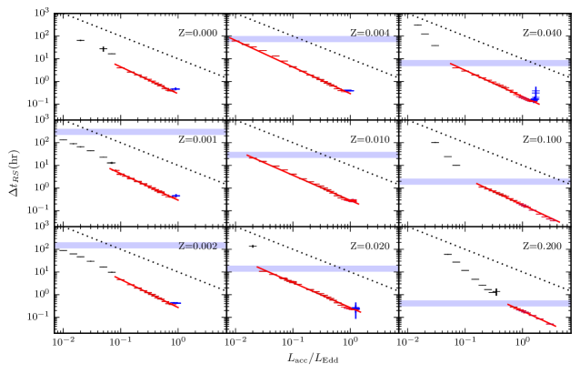
Figure 1.— Burst recurrence time ($\Delta t_{RS}$) as a function of accretion rate for different accreted metallicities, redshifted by $z=1.26$ to an observer’s frame. Error bars show the $1-\sigma$ variation of $\tau$ for a given composition. During mixed H/He bursts (case III, red points) the relationship between accretion rate and recurrence time is well described by a power law (red line) for all metallicities. Simulations of case II (blue) and case IV (black) burning are also plotted, whilst the shaded region indicates the time for hydrogen to be depleted by the hot CNO cycle. The transition to case IV burning is expected to occur within this shaded region. For metallicities of $\mathrm{Z}\leq 0.002$ we do not fit for $\mathrm{\dot{M}}<1.4\times 10^{-9}\,\mathrm{M_{\odot}}\,\mathrm{yr^{-1}}$ as bursts show an extended tail which prolongs $\Delta t$. Note that we exclude bursts with a recurrence time less than $\Delta t=100\,\mathrm{s}$ as the burst duration approaches the recurrence time. This does occur at high accretion in the $\mathrm{Z}=0.10$ and $\mathrm{Z}=0.20$

cases. Each plot has an identical power law with a gradient of $\eta=1.0$ plotted for comparison.

The relationship between accretion rate and recurrence time has been well studied for a number of sources, including GS 1826$-$24 (Galloway et al., 2004; Thompson et al., 2008) and MXB 1730$-$335, also known as the rapid burster (Bagnoli et al., 2013). Observationally, a power law relationship has frequently been found, relating the persistent flux, ($f_{\mathrm{pers}})$ of the source to the burst recurrence time, with the form

$$\Delta t\propto f_{\mathrm{pers}}^{-\eta}.$$ (7)

The persistent flux of a neutron star is primarily due to an energy deposition of $Q_{\mathrm{grav}}\mathrm{g}^{-1}$ from accretion onto the star. For a star of radius $R$ at a distance $d$ the flux (given an anisotropy of $\xi_{\mathrm{pers}}$) is given by

$$f_{\mathrm{pers}}=\frac{L_{\mathrm{pers}}}{4\pi d^{2}}=\frac{\dot{m}Q_{\mathrm{grav}}}{1+z}\left(\frac{R}{d}\right)^{2}\xi_{\mathrm{pers}}^{-1},$$ (8)

and hence ideally, the persistent flux is directly proportional to the mass accretion rate. It then follows that variations in recurrence time are due to changes in the accretion rate,

$$\Delta t\propto\dot{m}^{-\eta}.$$ (9)

Naïvely, we can expect the power law gradient to be $\eta\sim 1$ if we assume that a constant critical mass $m_{\mathrm{crit}}$ is required for a burst, as $\Delta t=m_{\mathrm{crit}}/\dot{m}$. Deviations from this relation suggest that the mass necessary for an instability varies with accretion.

For each accretion composition in Table 2, we identified model runs that exhibit five or more bursts, and fitted power laws for the variation in recurrence time with accretion rate across the region of case III burning. Recurrence times were redshifted by $z=0.26$, to be observationally equivalent to a ${M}=1.4\,\mathrm{M_{\odot}}$, $r=11.2\,\mathrm{km}$ neutron star. We excluded models where $\Delta t<100\,\mathrm{s}$, though this only occurs for $Z\geq 0.10$. The best fit power law was found via a $\chi^{2}$-minimisation, using the variation in recurrence time throughout the model run to weight each point. At the high accretion rate end of the power law, we stopped fitting when the recurrence time stopped decreasing. At the low accretion rate end, we stopped fitting when the points followed a noticeably different linear trend in log-log space (noting that the nature of the deviation changes with metallicity). For metallicities $z=0.020$ and above, this transition corresponds to a change in the burst behaviour, from the long-tailed lightcurve morphology (characteristic of mixed H/He bursts) to an Eddington-limited lightcurve caused by pure He bursts. For these runs, the power law fit spans the entire range of case III burning. The linear relationship becomes considerably steeper in the pure He bursting region. In the low metallicity cases ($z=0.000,\ z=0.001\,\mathrm{and}\ z=0.002$), mixed H/He burning still continues at accretion rates below where the power law stops being fitted, as the trend is translated vertically up for $l_{\mathrm{acc}}<0.08$. The value of $\eta$ and its associated 1-$\sigma$ uncertainty from the $\chi^{2}$ minimisation are shown in Table 3, and the actual data and fits are shown in Figure 1, with the fitted points plotted in red.

We find that in the KEPLER models, the value of $\eta$ depends upon the stellar composition and accretion rate. Using the recurrence times derived from our analysis of the model catalog we find that the variation with accretion rate is consistent with a power law across a wide range of accretion rates and metallicities.

There is no significant correlation between power law index and metallicity (Spearman $\rho=-0.48$, $p=0.187\approx 1.3\sigma$). Interestingly, all metallicities show $\eta\gtrsim 1.1$ whilst observations do not show such steep gradients. Galloway et al. (2004) find $\eta=1.05\pm 0.02$ for GS 1826$-$24 whilst Bagnoli et al. (2013) find $\eta=0.95\pm 0.03$ for MXB 1730$-$335. Linares et al. (2012) find that the X-ray pulsar IGR J17480$-$2446 shows $\eta\approx 1$ when $L_{\mathrm{pers}}>0.3L_{\mathrm{Edd}}$, and $\eta\approx 3$ when $0.2L_{\mathrm{Edd}}<L_{\mathrm{pers}}<0.3L_{\mathrm{Edd}}$. The assumption that the burst anisotropy is independent of accretion rate is necessary to compare observational and theoretical power law indices. It is likely however that there are burst behaviours that violate this assumption.

We found that models with 1% and 2% metallicity come closest to the observed $\eta$ values ($\eta\approx 1.11$). It would however be overstating the available evidence to suggest this implies that the observational sources discussed in the preceeding paragraph are consequently metal rich, as modelled power laws could be systematically high. It is nevertheless notable that metallicities around solar show a minimum $\eta$ value in the parameter range tested, suggesting that if a large sample of power law gradients were compiled, the lowest gradients would correspond to metal-rich population I stars.

Using theoretical burst ignition models, Galloway et al. (2004) found $\eta<1$ for solar metallicities, with $\eta$ increasing as metallicity drops. The KEPLER models show noticeably higher power law indices than this, though the trend for steeper power laws to be found at lower metallicities is replicated. Part of the reason for our disagreement with these models is that the models used in Galloway et al. neglect additional heating of the atmosphere by accumulated CNO, leading to systematic differences to KEPLER.

Z	$\eta$	n	$l_{\mathrm{acc,\,IV}}$	$l_{\mathrm{acc,\,III}}$	$l_{\mathrm{acc,\,II}}$
0.000	$1.19\pm 0.03$	10	$\cdots$	$0.75$	$0.92$
0.001	$1.17\pm 0.02$	21	$\cdots$	$0.80$	$0.92$
0.002	$1.237\pm 0.014$	10	$\cdots$	$0.80$	$0.97$
0.004	$1.17\pm 0.02$	16	$\cdots$	$0.80$	$1.00$
0.010	$1.109\pm 0.006$	32	$\cdots$	$1.10$	$1.11$
0.020	$1.106\pm 0.016$	21	$0.03$	$1.20$	$1.26$
0.040	$1.16\pm 0.02$	19	$0.07$	$1.55$	$1.71$
0.100	$1.18\pm 0.02$	17	$0.20$	$4.20$	$4.20$
0.200	$1.16\pm 0.02$	7	$0.70$	$6.50$	$7.50$
N&H03			$0.04$	$0.15$	$0.25$
F81			$0.08$	$\cdots$	$1.0$

Table 3The power law index $\eta$ for the power laws fitted to case III burning in Figure 1 are shown here for each metallicity along with the number of fitted points, $n$. The power laws were found following a $\chi^{2}$ minimisation of equation 9 with respect to the data each data set. The accretion luminosities (in terms of $l_{\mathrm{Edd}}$) where burning transitions occur are also shown for each metallicity. The transition times of Narayan & Heyl (2003) are reprinted from Table 1 with the transitions predicted by Fujimoto et al. (1981) also, who do not distinguish case IV from steady burning. .

We find also that the transition accretion rates, where the burning regime changes, increase with metallicity (Table 3). The transition accretion rates are defined where the burst behavior of the model changes in a qualitatively similar way to that defined by the burst cases presented by Narayan & Heyl (2003). We denote $l_{\mathrm{acc,\ IV}}=L_{\mathrm{acc,\,IV}}/L_{\mathrm{Edd}}$ as the accretion luminosity (in terms of Eddington) as the lowest accretion luminosity at which we observe case III bursts. $l_{\mathrm{acc,\,III}}$ denotes the accretion luminosity at which the shortest recurrence time is observed, and $l_{\mathrm{acc,\,II}}$ denotes the highest accretion rate for which we observe bursts. KEPLER simulations produce roughly similar transition accretion rates as stability analyses suggest, noting that both Fujimoto et al. (1981) and Narayan & Heyl (2003) consider solar accretion compositions.

Fujimoto et al. (1981) consider three neutron star potentials, all significantly different from the surface gravity adopted in KEPLER. Of the two closest to our considered surface gravity, the first overestimates the surface gravity by $\sim 55\%$ ($M=1.00\,\mathrm{M_{\odot}}$, $r=7.49\,\mathrm{km}$), whilst the second underestimates it by $\sim 35\%$ ($M=0.476\,\mathrm{M_{\odot}}$, $r=8.67\,\mathrm{km}$). These analyses predict $l_{\mathrm{acc,\,IV}}=0.08$ for the higher gravity, and $l_{\mathrm{acc,\,IV}}=0.03$ for the lighter gravity. We find $l_{\mathrm{acc,\,IV}}=0.03$ for $Z=0.02$, agreeing with the lower surface gravity case. Narayan & Heyl (2003) analysed the stability of burning on a star with only a 20% ($M=1.40\,\mathrm{M_{\odot}}$, $r=10.0\,\mathrm{km}$) higher surface gravity than KEPLER using a more rigorous approach, finding $l_{\mathrm{acc,\,IV}}=0.04$. Whilst each study uses different surface gravities, our value for the transition rate from case IV to case III burning broadly agrees with earlier stability analyses.

Despite this, the transition from case III to the case II and I regimes occurs at noticeably higher accretion rates than predicted by Narayan & Heyl (2003). We instead find these changes occur near $l_{\mathrm{acc}}\sim 1.2$, rather than the $l_{\mathrm{acc}}\sim 0.25$ predicted by Narayan & Heyl (2003). This is in closer agreement to Fujimoto et al. (1981) who find that the transition to stable burning occurs at $l_{\mathrm{acc}}\sim 1$ regardless of surface gravity. Additionally, case II burning occurs in general over a smaller range of accretion rates than Narayan & Heyl (2003) predict, however our method of choosing when case III burning transitions to case II arguably misses part of the case II region. This is most noticed in the $Z=0.01$ runs as case II burning shows oscillations in recurrence rate that increase the burst rate to faster than case III burning. Whilst in general the minimum recurrence time provides an approximate measurement of the case III to case II transition, burning compositions and burst morphologies would be more robust.

The general shape of the $\dot{m}-\Delta t$ relationship outside of the region of case III burning follows the predictions of Narayan & Heyl (2003), with a turnup where overstable burning commences, and a steeper power law index in the pure He bursting regime. In the overstable burning regime (case II) the recurrence time increases with accretion rate as a large proportion of the accreted fuel is being burnt during accretion. As both hydrogen and helium are burnt quickly in this regime a longer time is required to accrete sufficient fuel for a burst to occur. The turnup is relatively small within the KEPLER simulations, increasing the recurrence time by a fraction of an hour. This is in disagreement with the stability analyses of Narayan & Heyl (2003) who find that the recurrence time may increase by up to a day beyond the shortest recurrence times they observe. Whilst these two results are quantitively different, the upturn we observe does support qualitatively the overstable behaviour predicted for case II bursting.

The behaviour of the upturn is especially notable for the $Z=0.04$ case (Figure 2). Whilst the upturn is reasonably brief in most compositions, it shows substantial structure for this metallicity. Physically at these accretion regimes the increase in recurrence time is linked to helium in addition to hydrogen burning between bursts depleting the available fuel. In this regime luminosity between bursts tends not to fall quickly back to its persistent level. Interestingly, near $l_{\mathrm{acc}}\sim 1.65$ the uncertainty in $\Delta t$ becomes again small, similar to the case III uncertainties, and $\Delta t$ slightly decreases, before resuming its upward trend. In general, the large uncertainties in $\Delta t$ in this region are a consequence of metastable H/He burning, and the large impact small changes in the composition of the atmosphere can have on the stability of the accreted column. It is possible that in the intermediate area where $l_{\mathrm{acc}}\sim 1.65$ the column is slightly more stable, the exact reason for this will be investigated in more detail in the future

The steeper power law index in the region of pure He bursts is caused by the higher amount of accumulated helium required for a burst as compared to hydrogen, and the lack of heating from H burning. We could better constrain the power law behaviour in this region with more simulations at low accretion rates, however these typically require very long computation times per burst, as in the helium bursting regime more integration steps are needed per burst.

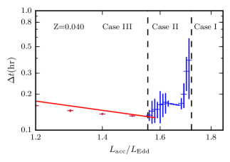
Figure 2.— The variation in recurrence time (plotted with $1-\sigma$ errorbars) with accretion rate for a star accreting fuel with $z=0.040$ near the steady burning transition (case II to case I). As burning transitions from stable H burning to overstable H/He burning, the recurrence time abruptly begins to increase with accretion rate. The increase in recurrence time is attributable to the increased rate of steady burning of the accumulated fuel leading to a longer time required for a critical density to be reached.

3.2. Transitions from pure He to mixed H/He bursts

The transition between case IV (pure He) burning and case III (mixed H/He) burning is expected to cause a significant change in the recurrence time due to the higher temperatures required for runaway helium burning. This leads to a discontinuity in the $\Delta t-\dot{m}$ relationship at accretion rates low enough for the accreted hydrogen to be depleted by hot CNO burning between bursts.The discontinuity occurs at a recurrence time similar to the time for the hot CNO cycle to deplete all hydrogen present. Fujimoto et al. (1981) express this relation as $\Delta t=9.7\,\mathrm{hr}\,(\mathrm{Z}/0.02)^{-1}$ in the neutron star frame, whilst Galloway et al. (2004) suggest $\Delta t=11\,\mathrm{hr}\,(\mathrm{H}/0.02)^{-1}(\mathrm{H}/0.7)$. We attribute the discrepancy in the Galloway et al. expression due to it’s adaptation of an earlier calculation in Bildsten (1998) that fails to incorporate neutrino energy losses in the hot CNO cycle. Given this difference however, we provide an independent derivation of this relationship below, laying out the assumptions inherent within it.

The hot CNO cycle (Mathews & Dietrich, 1984) occurs when temperatures are sufficiently high for proton capture by $\ce{{}^{13}N}$ to occur more frequently than $\ce{{}^{13}N}$ undergoes $\ce{\beta^{+}}$ decay. This leads to the hot CNO reaction cycle

$$\ce{{}^{12}C}(p,\gamma)\ce{{}^{13}N}(p,\gamma)\ce{{}^{14}O}(\ce{\beta^{+}}\nu)\ce{{}^{14}N}(p,\gamma)$$

$$\ce{{}^{15}O}(\ce{\beta^{+}}\nu)\ce{{}^{15}N}(p,\alpha)\ce{{}^{12}C}$$ (10)

The cycle is limited by the $\ce{\beta^{+}}$ decay of $\ce{{}^{14}O}$ and $\ce{{}^{15}O}$. To find the time to burn all available hydrogen, we consider that each decay of $\ce{{}^{14}O}$ in the cycle requires four proton captures. This gives the burning rate of $\ce{{}^{1}H}$ as follows:

$$\partial_{t}\mathrm{Y}_{\ce{{}^{1}H}}=-4\frac{\ln{2}}{t_{\frac{1}{2},\ce{{}^{14}O}}}\mathrm{Y}_{\ce{{}^{14}O}}.$$ (11)

Integrating this expression with the initial condition that $\mathrm{Y}_{\ce{{}^{1}H}(t=0)}=\mathrm{Y}_{\ce{{}^{1}H}}^{\mathrm{init}}$ and and finding when the hydrogen is depleted gives the time taken to burn an accumulated fuel layer by the hot CNO cycle,

$$t_{\mathrm{CNO}}=\frac{\mathrm{Y}_{\ce{{}^{1}H}}^{\mathrm{init}}}{\mathrm{Y}_{\ce{{}^{14}O}}}\cdot\frac{t_{\frac{1}{2},\ce{{}^{14}O}}}{4\ln{2}}$$ (12)

In the hot CNO cycle, the reaction rate is restricted by the beta decay of $\ce{{}^{14}O}$ and $\ce{{}^{15}O}$, so at any point the majority of CNO is in these two isotopes, meaning $\mathrm{Y}_{\ce{{}^{14}O}}+\mathrm{Y}_{\ce{{}^{15}O}}\approx\mathrm{Y}_{\mathrm{CNO}}$. Noting that $Y(\ce{{}^{14}O})/Y(\ce{{}^{15}O})=t_{\frac{1}{2},\ce{{}^{14}O}}/t_{\frac{1}{2},\ce{{}^{15}O}}$ the number fraction of $Y(\ce{{}^{14}O})$ is expressible in terms of the CNO abundance:

$$\frac{\mathrm{Y}_{\ce{{}^{14}O}}}{\mathrm{Y}_{\mathrm{CNO}}}\approx\frac{\mathrm{Y}_{\ce{{}^{14}O}}}{\mathrm{Y}_{\ce{{}^{14}O}+\mathrm{Y}_{\ce{{}^{15}O}}}}=\frac{t_{\frac{1}{2},\ce{{}^{14}O}}}{t_{\frac{1}{2},\ce{{}^{14}O}}+t_{\frac{1}{2},\ce{{}^{15}O}}}.$$ (13)

Proceeding now from equation 12, the CNO burning time can be expressed as

$$t_{\mathrm{CNO}}=\frac{\mathrm{Y}_{\ce{{}^{1}H}}}{\mathrm{Y}_{\mathrm{CNO}}}\cdot\frac{t_{\frac{1}{2},\ce{{}^{14}O}}+t_{\frac{1}{2},\ce{{}^{15}O}}}{4\ln{2}}.$$ (14)

Conversion of $\mathrm{Y_{CNO}}$ to a metallicity mass fraction requires assumptions about the composition in order to find the mean molecular mass. Assuming that all of the accreted metals are in CNO with their solar ratios (Asplund et al., 2009) the number fraction $\mathrm{Y_{CNO}}=\mathrm{Z}/\bar{\mu}_{\mathrm{CNO}}$, with $\bar{\mu}_{\mathrm{CNO}}=14.5\,\mathrm{g}\,\mathrm{mol^{-1}}$ Substituting the half-lives of both oxygen species ($t_{\frac{1}{2},\ce{{}^{14}O}}=71\,\mathrm{s}$ and $t_{\frac{1}{2},\ce{{}^{15}O}}=122\,\mathrm{s}$) the hydrogen burning time is given by

$$t_{\mathrm{CNO}}=9.8\,\mathrm{hr}\left(\frac{\mathrm{H}}{0.7}\right)\left(\frac{\mathrm{Z}}{0.02}\right)^{-1},$$ (15)

noting that the prefactor is within the precision of Fujimoto et al. (1981), a difference that could be accounted for by a small change in the measurement of $\bar{\mu}_{\mathrm{CNO}}$ used. This prefactor can show some variability depending on what the metal component is assumed to be (noting that this variability comes from using an expression based on mass rather than number fraction). For example, assuming purely $\ce{{}^{16}O}$ ($\ce{{}^{14}N}$, $\ce{{}^{12}C}$) leads to a prefactor of $10.8\,\mathrm{hr}$ ($9.5\,\mathrm{hr}$, $8.1\,\mathrm{hr}$). Additionally, as the CNO fraction does not typically comprise all the metallicity within a star, $9.8\,\mathrm{hr}$ is likely an underestimate for the CNO burning time. For solar composition (Asplund et al., 2009), only 66% of the metals (by mass) are CNO. Taking this into consideration the prefactor increases to $15\,\mathrm{hr}$ in the neutron star frame. We do not expect the KEPLER models to be best modelled by this last case as the metallicity component accreted is entirely $\ce{{}^{14}N}$ rather than solar.

In runs at metallicities of $\mathrm{Z}=0.02$ and higher, pure He bursts, indicated by photospheric radius expansion, are observed at low accretion rates (blue points at the low accretion end of the power law in Figure 1). For each composition, we expect the power law that describes case III burning to have an upper bound in recurrence time for each composition to be described by the hot CNO cycle hydrogen burning time (Equation 12). For $\mathrm{Z}=0.02\ (0.04,\ 0.10,\ 0.20)$ this time is $\Delta t=12\ (5.7,\ 1.7,\ 0.4)\,\mathrm{hr}$ after redshifting by $1+z=1.26$. In each model run we observe case III burning at recurrence times shorter than the hot CNO burning time and case IV burning above these times, as expected.

This agreement is also noticed using the $11\,\mathrm{hr}$ prefactor suggested by Galloway et al. (2004). The modelled results in Galloway et al. (2004) have a redshift of $1+z=1.31$, leading to a rest frame prefactor of $8.4\,\mathrm{hr}$. Such a value could arise from accretion if most of the metallicity fraction is carbon. Most of the suggested prefactors thus far match our simulated data. Figure 1 shows in blue shading to highlight the range of times wherein the CNO cycle is expected to deplete available hydrogen, using the unredshifted prefactors of $8.1\,\mathrm{hr}$ and $15\,\mathrm{hr}$ as limits. Only the low end ($\lesssim 9\,\mathrm{hr}$) of this range is excluded by the KEPLER models.

Considering all this detail, we emphasise the approximate nature of equation 15. Changes in accretion composition, gravitational redshift and the presence of ashes from previous bursts can foreseeably combine to greatly vary this prefactor. Increasing the resolution of simulations in accretion rate in order to better isolate the transition from case IV to case III burning may lead to a better determination of the prefactor (given the assumptions within KEPLER) and also allow some quantification of the deviation CNO ashes cause from the theoretical prefactor. However as observational systems have significantly greater deviations from theory than KEPLER, better constraints are unlikely to be very useful.

3.3. Recurrence time behaviour at low metallicity

For models run at metallicities lower than $Z=0.02$, no runs show case IV burning, as they do not span accretion rates low enough to deplete all the available hydrogen. Rather, a noticeable vertical translation of the power law index occurs for accretion rates with $l_{\mathrm{acc}}\lesssim 0.08$. To determine the significance of this deviation we considered the $\chi^{2}_{\nu}$ for fits to the recurrence time versus the accretion rate, across both the range of accretion rates from $l_{\mathrm{acc}}=0.08$ to the case II transition, and for all accretion rates up to the case II transition. For $Z=0.002$ ($Z=0.001$, $Z=0.0$) we found that using the larger fitting range drastically increased the $\chi^{2}_{\nu}$ from 0.98 (2.65,3.36) to 21.8 (33.0, 29.5). Whilst these fits are phenomenological and a high $\chi^{2}$ may occur on account of this, the variation in these two fits suggests that at accretion rates $l_{\mathrm{acc}}\lesssim 0.08$ the power law that describes these bursts is different.

To this end, we examined the morphology of bursts at this low accretion rate, noticing that there is a change in the structure of the burst tail at accretion rates lower than where we cease fitting. At such low accretion rates, the burst lightcurve shows a two stage decay (Figure 3) rather than a single decay. The presence of a second decay, reached after the first decay flattens indicates an additional burning process, which could act to consume additional fuel, thereby extending the accretion time required to recuperate an unstable column. Further investigation into the nuclear networks active in KEPLER during these bursts, as well as the rapidity of the onset of the two stage decay, could present an interesting avenue for further study.

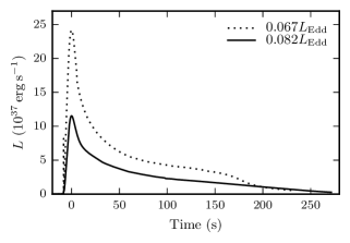
Figure 3.— In low metallicity sources a significant change in morphology to occurs near $L_{\mathrm{acc}}\sim 0.07L_{\mathrm{Edd}}$ ($\mathrm{\dot{M}}\sim 10^{-9}\,\mathrm{M_{\odot}}\,\mathrm{yr^{-1}}$) whereby the bursts become brighter and show a decay in the tail consisting of two stages. The two models shown were run at $Z=0.001$ and have accretion rates of $L_{\mathrm{acc}}=0.067L_{\mathrm{Edd}}$ (dotted, model a20) and $L_{\mathrm{acc}}=0.067L_{\mathrm{Edd}}$ (solid, model a30). Luminosities and times are in the NS frame.

3.4. Recurrence time variation with $\tau$

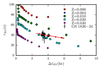
Figure 4.— The recurrence time and equivalent duration $\tau_{RS}$ (redshifted to the observer’s frame) of a burst are observable phenomena that vary with accretion rate. Here, accretion rate increases from right to left. Red circles, blue pentagons, green diamonds, teal squares and purple hexagons represent model runs with $\mathrm{Z}=0.000,\ 0.004,\ 0.010,\ 0.020\ \mathrm{and}\ 0.040$ respectively. The black points represent observations of the recurrence time and equivalent duration of GS 1826$-$24, and the associated 1-$\sigma$ error in equivalent burst duration. The red line is a linear fit to the observed data to illustrate the general observed trend. GS 1826$-$24 sits between the $\mathrm{Z=0.010}$ and $\mathrm{Z=0.020}$ models, following a shallower gradient than either.

Both equivalent burst duration ($\tau$) and recurrence time ($\Delta t$) are commonly used observational measures in burst studies. Importantly, both measures are independent of distance. As such, the loci traced by simulated bursts in $\tau-\Delta t$ space provides a series of curves which can be compared to observations (for an assumed gravitational redshift). This is considered in Figure 4, along with observed values of $\tau$ and $\Delta t$ for GS 1826$-$24. The simulated parameters have been redshifted by $1+z=1.26$, corresponding to a $1.4\,\mathrm{M_{\odot}}$ neutron star $11.2\,\mathrm{km}$ in radius.

We compared these simulated parameters to observations of GS 1826$-$24 for which we had a reliable recurrence time (determined from finding two bursts close in time). The values of recurrence time and $\tau$ for GS 1826$-$24 appear between the locus traced by the $\mathrm{Z}=0.01$ and $\mathrm{Z}=0.02$ models. This suggests an accretion metallicity slightly lower than $\mathrm{Z}=0.02$, in agreement with Heger et al. (2007a), although we note that their comparison also uses KEPLER models. The span of the observations corresponds to modelled accretion rates of $l_{\mathrm{acc}}=0.065$ to $l_{\mathrm{acc}}=0.123$. To illustrate the behaviour of GS 1826$-$24 we have fitted a linear model ($\tau=A\Delta t+B$) to the observations by $\chi^{2}$-minimisation, finding $A=-2.8\pm 0.3\,\mathrm{s}\,\mathrm{hr^{-1}}$ and $B=50\pm 1\,\mathrm{s}$ ($\chi^{2}_{\nu}=1.2$).

Interestingly, the gradient from the GS 1826$-$24 observations in Figure 4 shows a shallower drop in $\Delta t$ with $\tau$ than the modelled points. As higher recurrence times are indicative of lower accretion rates, we see higher fluences than KEPLER predicts as accretion rate drops. The deviation from the locus of $\mathrm{Z}=0.02$ is largely driven by the three data points at recurrence times $>5\ \mathrm{hr}$. Whilst it could be tempting to to eliminate these points as examples of non-standard behavior of the star, recent observations of GS 1826$-$24 have shown the star exhibiting an uncharacteristic soft spectral state (Chenevez et al., 2015), strengthening the idea that these points reflect the behavior of GS 1826$-$24, and that its behavior is thus not in accordance with that predicted by KEPLER for $Z=0.02$ accretion. Part of the reason for this may be in that the accretion regime used by us, whereby only $\ce{{}^{14}N}$ is being accreted, does not provide adequate seed nuclei to reproduce the behaviors of naturally occurring stars where a more diverse quantity of metals are accreted. It woud be interesting in further studies to investigate how variations in the accretion composition affect these loci.

4. Results and Discussion II: Morphological variations

A number of parameters have been used in the literature to quantify the morphology of a lightcurve. In models, these parameters can show significantly more variation in subsequent burst trains than is observed in some sources. In this section we summarise the broad trends in burst convexity, $\alpha$ and tail shape that we find in the KEPLER models, as well as the appearance of twin-peaked bursts.

4.1. Burst to burst variation within a train

A recurring puzzle in the morphologies of modelled bursts is their variablility. Naïvely, models would be expected to show relatively uniform bursts (apart from the first few bursts in a simulation) as the composition of the neutron star atmosphere approaches a steady level. This is seen to some extent: the first burst in a train is disproportionately energetic, and the following bursts show variations of about 10% between the peak luminosity of the brightest and the dimmest.

This behavior implies that there is a natural variability in burst lightcurves that arises from nuclear physics, yet some observational sources, notably GS 1826$-$24, do not show as much variability within a burst epoch as simulated bursts show within a model run. We suggest that this is due to the number of convective cells on a bursting neutron star collectively removing the variation we see in the models. Each model effectively assumes the neutron star contains a single convective cell. Rather, assuming a cell diameter similar to the atmosphere height ($\sim 10\,\mathrm{cm}$), a neutron star has on the order of $10^{7}$ convective cells. This would produce a lightcurve equivalent to the average of $10^{7}$ modelled bursts and thereby suppress the variations in burst behavior that are caused by nuclear physics.

4.2. Convexity

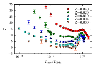
Figure 5.— Convexity increases for a given accretion rate as metallicity increases. In general, it decrases with accretion, though it flattens in the region $0.1\lesssim l_{\mathrm{acc}}\lesssim 1.0$. Here, errorbars represent the $1\sigma$ variation in convexity within a model run. Notably, convexity shows little variation within a model run in most cases.

Variations in the shape of the burst rise can be expected as a function of the latitude on the neutron star at which the burst commences; nuclear processes; burst spreading; and also a contribution from scattering within the accretion disk. The KEPLER models simulate nuclear processes without simulating accretion disk interactions or ignition latitude, allowing the contribution of nuclear burning to burst convexity to be determined.

For our discussion of convexity we restrict the sample to bursts with a metallicity of $Z\leq 0.04$, that exhibit a smooth rise. This excludes many PRE bursts as these often exhibit sudden increases in luminosity from convective zones rising to the stellar surface as burning commences. Bursts from runs with higher metallicities were excluded as their convexities are skewed by the development of two peaks in the rise (see §4.5).

Figure 5 shows the variations in burst convexity with both accretion rate and metallicity. For metallicities less than $Z=0.002$, the convexity changes very little as the accretion luminosity changes from $0.1\,L_{\mathrm{Edd}}$ to $0.6\,L_{\mathrm{Edd}}$. Across this range the convexity rises with increasing metallicity, from near $\mathcal{C}=1\%$ for $Z=0.000$ to $\mathcal{C}=9\%$ for $z=0.020$. Above $0.6\,L_{\mathrm{Edd}}$ bursts with metallicities below solar converge towards $\mathcal{C}=2\%$.

Very few ‘concave’ bursts ($\mathcal{C}<0$) are observed in the KEPLER sample. Rather $Z=0.0$ bursts have $\mathcal{C}=0\%$ and convexity increases with metallicity. Variations in convexity within a run are small, with the mean uncertainty typically on the order of one percentage point. The burst-to-burst variation in convexity increases at high accretion rates, correlated with the onset of case II burning, and also at low accretion rates, where a larger amount of the accreted hydrogen is depleted.

The KEPLER models show a far more constrained range of convexities within a run than those observed in single sources. Following Maurer & Watts (2008), we find the mean convexity of 4U 1636$-$536 to be $\mathcal{C}_{\mathrm{avg}}=4.7\%$, with a $1\sigma$ spread of 10.8 percentage points, across a large range of persistent emissions. Even within a restricted range of persistent flux ($2\times 10^{-9}\,\mathrm{erg}\ \mathrm{cm^{-2}}\,\mathrm{s}<f_{\mathrm{pers}}<3\times 10^{-9}\,\mathrm{erg}\ \mathrm{cm^{-2}}\,\mathrm{s}$) the spread in convexities is still notably larger than nuclear burning predicts. We also consider the variation in convexity shown by GS 1826$-$24 as it is known for showing consistent lightcurves dominated by nuclear processes (Heger et al., 2007a). GS 1826$-$24 shows a narrower distribution of convexities with $\mathcal{C}_{\mathrm{avg}}=4.1\pm 2.9\%$, though the distribution of convexities is again wider than a single run would on average predict. Note that the error in observational convexity values here does not consider the error in convexity from each observation as it is markedly smaller. We calculated this using the observed flux $\pm 1\sigma$, and found that for 4U 1636$-$536 and GS 1826$-$24, these varied on average by 0.7 and 0.3 percentage points from the convexity value calculated using the mean flux.

The larger spread in convexity for observations is in part due to the span of persistent fluxes (and thereby accretion rates) covered by observations, as convexity does show some variation with accretion rate. For both GS 1826$-$24 and 4U 1636$-$536, this is insufficient to explain the full range in convexities spanned by both sources. 4U 1636$-$536 shows convexities ranging from $\mathcal{C}\approx-30\%$ to $\mathcal{C}\approx 40\%$. No single composition shows this amount of variation in convexity across the range of accretion rates simulated, and nuclear burning does not produce noticeably concave bursts. Hence it is likely that physical processes (e.g. spreading) on the neutron star have a more significant impact upon the burst rise in 4U 1636$-$536 than nuclear processes.

GS 1826$-$24  shows a far more constrained range of convexities than 4U 1636$-$536, however the observed dispersion in convexities is still more than typical within the models. This indicates that the physical processes that influence convexity are far more constrained in the GS 1826$-$24 system than in 4U 1636$-$536. In their comparison of GS 1826$-$24 to KEPLER models, Heger et al. (2007a) find that GS 1826$-$24 is likely accreting fuel with a solar metallicity at $\dot{{M}}=1.58\times 10^{-9}\,\mathrm{M_{\odot}}\ \mathrm{yr^{-1}}$. The predicted convexity from this comparison ($\mathcal{C}\approx 11\%$) however is higher than is observed. This could indicate a physical process on GS 1826$-$24 that reduces the convexity in the rise, such as ignition at a certain latitude and burst spreading, or it could be due to systematic uncertainties in the KEPLER models.

4.3. Burst energetics

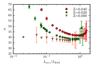
Figure 6.— The ratio of persistent fluence to burst fluence ($\alpha$) increases with metallicity. For metallicities of $Z\leq 0.02$, $\alpha$ remains mostly constant across case II burning, showing an increase as the hydrogen depletes. Near metastable burning the value of $\alpha$ becomes less consistent as the burst fluence becomes more variable, and the recurrence time approaches a similar magnitude to the burst duration.

We find $\alpha$ predicted by KEPLER models match the range of $\alpha$ seen observationally, with $\alpha\approx 40$ in the region $0.1\lesssim l_{\mathrm{acc}}\lesssim 1.0$. In general, $\alpha$ tends to grow with metallicity (Figure 6). At high accretion rates, variations in $\alpha$ between bursts obscure this trend, as fluence measurements become more variable when the recurrence time is of a similar order of magnitude to the burst duration (typically 10% to 50% of $t_{b}$). The variation in $\alpha$ with accretion rate matches the expected trends for each metallicity, being approximately flat for no metallicity and increasing in curvature with metallicity following Galloway et al. (2004). For the data points with zero metallicity, the uncertainties at low accretion rates are sometimes very large, this is a manifestation of large variations in peak luminosity and recurrence time between bursts, which is accentuated in the cases where large uncertainties are seen.

4.4. Tail morphology

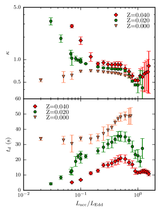
Figure 7.— As accretion rate increases, the power law index $\kappa$ of a power law fitted to the burst tail decreases, whilst the exponential decay time of the tail, $t_{d}$ increases. At higher metallicities the power law index increases at low accretion rates, whilst the decrease at low accretion rates is a consequence of increasingly poor fits due to a two-stage decay in the lightcurve.

The tails of thermonuclear bursts can yield information about the cooling processes within the star, as well as providing a metric to enable comparisons with observations. We found that the power law index that best describes a burst tail increases dramatically at low accretion rates, as hydrogen is depleted and helium becomes more prevalent in a burst. This is quite noticeable at $Z=2\%$ and $Z=4\%$ (Figure 7). In PRE bursts, similiarly high power laws were found. If the heat in the burst is lost by radiation and the specific heat capacity is independent of temperature, the expected power law gradient is $\kappa=4/3$ (in’t Zand et al., 2014), although an extended $rp$-process in the burst tail will obscure this cooling. This behaviour is especially noticeable in the zero metallicity case, where artificially low power laws are caused by a two stage decay (see Figure 3). At low accretion rates where extended $rp$-process burning is minimal, power law gradients approach $\kappa=3$ and can be as high as $\kappa=6$ for some PRE bursts. Such high power laws can be caused by degenerate photons and electrons influencing the specific heat capacity of the atmosphere at high energies.

Across most of the range of case III burning, little variation in $\kappa$ is observed with accretion rate(Figure 7), whilst the burst decay time increases. This is likely a consequence of the self-similarity of power laws with scaling. The trend we see suggests increased accretion leads to longer bursts with a similar decay power-law.

For metallicities of $Z=0.02$ and higher, the uncertainty in the power law constant grows considerably. This occurs as a result of the burst morphology showing large burst to burst variations as the burst duration grows similar to the recurrence time. In most morphological parameters, the measurements tend to show large burst to burst variations in the parameter value once the burst duration exceeds $\approx 10\%$ of the recurrence time.

4.5. Double-peaked bursts

Using the KEPLER simulations the nuclear origins of twin peak bursts can be investigated. As noted in simulations by Fisker et al. (2004), where two peaks occur, the first peak (which we refer to as the helium peak) arises from the rapid combustion of a helium layer at the bottom of the neutron star atmosphere, which convects rapidly to the surface, causing a large increase in surface brightness. The second peak (hereafter the primary peak) occurs due to a stalling of the $rp\mathrm{-process}$ at a nuclear waiting point. Notably, when there is insufficient helium accumulated deep in the neutron star atmosphere the peaks merge to create a typical mixed H/He burst.

In the KEPLER models, twin peaked structures are prominent in the higher metallicity models ($z=0.10$) at low accretion rates (Figure 8), whilst the helium peak is suppressed at higher accretion rates, manifesting as a distinct two stage rise. Of the two peaks present at $z=0.10$ the helium peak is larger than the primary peak at low $\dot{m}$, and also rises faster ($\sim 1\,\mathrm{s}$) than it does at higher accretion rates ($\sim 3\,\mathrm{s}$), bearing a slight resemblance to the quick rise of a helium flash. At solar metallicities the helium peak is not present as a local maximum but manifests rather as a kink in the burst rise (Figure 9) that is suppressed as accretion rate increases. In the intermediate case ($z=0.04$) the helium peak is present at low accretion rates, though the models tranisition to pure He bursts before the helium peak grows to be equal in magnitude to the primary peak. For each case discussed, the burst train throughout the models consistently show similar structures (twin-peaked or kinked) beyond the first few bursts in each train, which is markedly different to observations, where multi-peaked bursts rarely occur regularly. We have plotted the 11th burst for each simulation in Figures 8 and 9 to ensure that a consistent ashes layer has been found.

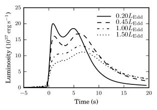
Figure 8.— Double peaked bursts show a dependance upon accretion rate, with the peak becoming more pronouned at higher accretion rates. The lowest accretion rates have the highest peak luminosity, with the solid, dashed, dot-dashed and dotted lines show the 11th burst from models with accretion rates of $L_{\mathrm{acc}}/L_{Edd}=0.20,\ 0.45,\ 1.00,\ \mathrm{and}\ 1.5$, accreting material with $z=0.10$.

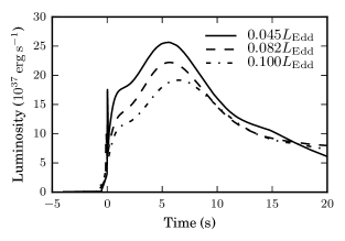
Figure 9.— At lower metallicities the double peak of Figure 8 is not observed, but appears as a kink in the burst rise that grows more dominant at lower accretion rates. Again, lower accretion rate models have higher peak luminosities. The solid, dashed and dot-dashed show the 11th burst from models with accretion rates of $L_{\mathrm{acc}}/L_{Edd}=0.045,\ 0.082\ \mathrm{and}\ 0.1$. The tendency of low accretion models to exhibit rapid increases in surface luminosity from hot convective regions rapidly rising to the surface is seen in the rise of the two lower accretion bursts.

The presence of twin peaked structures in our models indicates that double peaked structures can have a nuclear origin, however a larger than typical metallicity is required to produce these bursts consistently. The magnitude of the helium peak is largely dependant upon accretion rate. Lower accretion rates cause longer periods between bursts, depleting more hydrogen by hot CNO burning. The higher relative fraction of helium, especially at the base, leads to a more dominant initial helium powered rise.

The potential observability of a twin peaked burst however is not guaranteed as spreading of the lightcurve in time due to the propogation of the nuclear burning front may blur the peaks. In observational sources that show repeated peaks, multiple peaks are not observed with regularity, possibly due to their obfuscation by the propagating burning front. Also possible is that most observational sources do not accrete sufficiently metallic material to display a pronounced helium peak, however sometimes burning increases the local metallicity enough to cause occasional double peaked bursts as a consequence of compositional inertia.

5. Conclusion

In this study, we analysed the variations accretion rate and metallicity have upon measurable burst parameters with simulations run using KEPLER. We find the following conclusions:

1. Within the region of case III burning, recurrence time varies with accretion rate following a power law that varies with the metallicity of the accretion source.

2. The transition between pure He and mixed H/He bursts occurs at recurrence times consistent with hydrogen depletion via the $\beta$ limited CNO cycle.

3. Modelled parameters can be compared to observational values to ascertain accretion rate and composition.

4. Nuclear burning has an effect on burst convexity, however the variation seen observationally in the burst rise is greater than nuclear burning alone predicts, supporting its origin in burst location.

5. Nuclear burning can cause two peaks to arise in thermonuclear burst lightcurves when a significant amount of hydrogen has been depleted.

Appendix A Burst Analysis Flags

For each model run, the averaged parameters are presented in Table 4. Due to the variety of models analysed, any analysis issues are flagged using a binary code. The flags used are: 0, indicating no analysis issues; 1, indicating that a burst occurred as the simulation was finishing, and as such was not analysed; 2, indicating that due to convective shocks, the luminosity exceeded $10^{39}\,\mathrm{erg}\,\mathrm{s^{-1}}$ in the raw data, and the lightcurve was rebinned; 4, indicating that the end of the burst was triggered by reaching a local minimum; 8, indicating twin peaked bursts occur in the train; 16, indicating rapid bursts occur with recurrence time less than $100\,\mathrm{s}$; and 32, which indicates the raw data was too irregular for analysis.

The observable effect on burst parameters of flags 2 and 8 is a substantially poorer measurement of burst rise parameters, due to either convective shocks, or the presence of two peaks, causing ambiguity in the identification of a peak luminosity. Flag 4 is a consequence of metastable H/He burning extending the duration of a burst. In this case, the tail can sometimes show small follow-up bursts and oscillations in brightness. As these can extend the burst, as well as make the computation of an average burst difficult, they trigger the end of the burst. This however causes some of the burst fluence to be excluded from the meausrement, and as such, fluence parameters from models flagged 4 should be treated with caution, as they are likely to be slightly underestimated. The analysis for rapid bursts (flag 16) is quite robust, but there is a likelihood of a burst being missed. Additionally, these bursts arise from quite unlikely accretion compositions ($Z>0.10$).

Appendix B Comparison to observations

Here we briefly detail the conversion adopted used for comparisons to observations. These allow the models to be compared to a $1.4\,\mathrm{M_{\odot}}$ neutron star with a radius of $11.2\,\mathrm{km}$, within reasonable observational bounds for neutron star dimensions (Lattimer & Prakash, 2006). The gravitational potential within a neutron star atmosphere is sufficiently intense that general relativistic effects become relevant. As the neutron star atmosphere is small compared to the stellar radius, Newtonian gravity approximates general relativity well within the domain of the simulations, and all values provided in the database presented herein are in the Newtonian neutron star frame. Due to this approximation the lightcurves and parameters we provide require redshifting to be compared with observations.

A full derivation of all the possible scalings that can occur given a choice of stellar radius or mass is provided in the appendix of Keek & Heger (2011). The gravitational potential of our simulations is equivalent to the Newtonian potential that arises from body with a radius of $r=10\,\mathrm{km}$ and ${M}=1.4\,\mathrm{M_{\odot}}$ (note that quantities calculated in the Newtonian frame are unsubscripted). There is a plurality of masses ($M_{\mathrm{GR}}$) and radii ($r_{\mathrm{GR}}$) that could give rise to the same potential using general relativity. The locus of these points occurs where the Newtonian and GR potentials are equal:

$$GM/r^{2}=GM_{\mathrm{GR}}/\left(r_{\mathrm{GR}}^{2}\sqrt{1-2GM_{\mathrm{GR}}/(c^{2}r_{\mathrm{GR}})}\right).$$ (B1)

We have conducted our analysis for a neutron star that has the same mass as the star in the Newtonian simulations, choosing $M_{\mathrm{GR}}={M}=1.4\,\mathrm{M_{\odot}}$. Given this choice, the radius of the neutron star that give the same general relativistic potential increases, yielding $r_{\mathrm{GR}}=\xi r=11.2\,\mathrm{km}$, where $\xi=1.12$ (note that this is not the radius measured by a distant observer). The redshift can now be found using

$$1+z=1/\sqrt{1-2GM_{\mathrm{GR}}/(c^{2}r_{\mathrm{GR}})}=1.258.$$ (B2)

The relevant conversions for radius, luminosity, accretion rate, and time in this case for an observer (subscripted $\infty$), in terms of the Newtonian reference frame values, are:

$$r_{\infty} = \xi(1+z)r,$$

$$L_{\infty} = \xi^{2}\cdot L/(1+z)^{2},$$

$$t_{\infty} = (1+z)t,$$

$$\dot{{M}}_{\infty} = \dot{{M}},$$

$$\frac{L_{\mathrm{acc},\infty}}{L_{\mathrm{Edd},\infty}} = \frac{z}{\zeta(1+z)}\frac{L_{\mathrm{acc}}}{L_{\mathrm{Edd}}},$$

$$\alpha_{\infty} = \frac{z}{\zeta(1+z)}\alpha,$$ (B3)

where $\zeta=G{M}/(c^{2}r)$. A consequence of setting the GR mass equal to the Newtownian mass is that the mass accretion rate is identical in the Newtonian and observer frames. Additionally, this also yields $\xi=\sqrt{1+z}$, which simplifies a number of these relationships. The variation in $L_{\mathrm{acc}}/L_{\mathrm{Edd}}$ is attributable to the increased Eddington luminosity that arises from the strengthened GR potential.

It is also worth commenting that the scaling for $\alpha$ assumes only a contribution to the persistent emission from accretion. The radiation from persistent emission is redshifted in the same manner as burst luminosity. This can introduce a sytematic uncertainty into the calculation of a redshifted $\alpha$ if the accretion component is not calculated separately from the thermal component. As $L_{\mathrm{acc}}\gg L_{th}$ this is minimal, especially given that ${z}/{[\zeta(1+z)]}=0.9934$ given our choice of mass.

ID	Bursts	$Z$	$H$	$L_{\mathrm{acc}}/L_{\mathrm{Edd}}$	$t_{b}$	$L_{p}$	$L_{th}$	$E_{b}$	$\tau$	$\Delta t$	$\mathcal{C}$	$t_{10-90}$	$t_{25-90}$	$\kappa$	$t_{d}$	$\alpha$	Flag
$\cdots$	$\cdots$	$(10^{-9}\,\mathrm{M_{\odot}}\,\mathrm{yr^{-1}})$	$(\%$)	$(\%$)	$(\mathrm{s})$	$(10^{37}\,\mathrm{erg}\,\mathrm{s^{-1}})$	$(10^{35}\,\mathrm{erg}\,\mathrm{s^{-1}})$	$(10^{39}\,\mathrm{erg}\,\mathrm{s^{-1}})$	$(\mathrm{s})$	$(\mathrm{hr})$	$(\%$)	$(\mathrm{s})$	$(\mathrm{s})$	$\cdots$	$(\mathrm{s})$	$\cdots$	$\cdots$
a003	15	0.1	75.90	0.100	268.1	10.33	2.73	5.99	58.2	3.13	1.76	5.304	4.304	0.71	33.43	39.5	0
a004	4	0.1	75.90	0.020	213.1	29.50	0.70	19.10	64.8	53.97	7.82	5.570	4.819	0.72	35.08	43.2	0
a005	12	2.0	70.48	0.100	106.3	15.20	4.55	4.41	29.1	2.69	12.41	5.027	4.520	0.93	23.74	45.9	0
a006	8	2.0	70.48	0.020	54.8	52.18	1.26	8.04	15.5	108.27	38.60	0.360	0.347	5.82	3.19	196.1	2
a007	14	0.1	75.90	0.150	286.5	10.26	2.84	6.25	61.0	2.13	0.86	5.340	4.295	0.70	34.05	38.5	0
a008	21	0.1	75.90	0.500	367.9	7.04	4.98	5.44	77.3	0.53	0.64	5.866	4.683	0.65	47.50	36.5	0
a009	15	2.0	70.48	0.500	216.0	9.08	5.61	4.37	48.1	0.45	8.52	5.369	4.641	0.75	35.43	38.6	0
a010	6	0.0	76.00	0.020	337.1	21.49	0.55	18.94	88.1	51.49	4.93	5.475	4.454	0.53	33.71	40.1	0
a011	13	2.0	70.48	0.100	100.5	17.77	4.17	4.81	27.2	2.96	10.91	5.041	4.507	0.99	20.61	46.4	0
a012	3	2.0	70.48	0.015	71.4	49.18	0.73	10.12	20.6	131.09	0.00	0.064	0.052	4.59	4.53	149.0	2
a013	0	2.0	70.48	0.010	$\cdots$	$\cdots$	$\cdots$	$\cdots$	$\cdots$	$\cdots$	$\cdots$	$\cdots$	$\cdots$	$\cdots$	$\cdots$	$\cdots$	2
a014	10	2.0	70.48	0.030	36.9	25.73	3.40	2.92	11.3	8.48	29.23	3.501	3.370	3.26	4.23	67.9	2
a015	2	2.0	70.48	0.025	39.6	51.66	1.86	5.82	11.3	59.16	37.42	1.421	1.372	6.56	2.09	188.3	2
a016	1	4.0	65.00	0.020	77.3	47.25	0.65	10.61	22.5	$\cdots$	47.08	0.419	0.403	3.67	5.46	$\cdots$	2
a017	1	4.0	65.00	0.040	26.7	49.85	1.70	4.24	8.5	$\cdots$	0.00	0.076	0.064	7.64	1.66	$\cdots$	2
a018	1	4.0	65.00	0.050	27.0	49.50	4.37	3.75	7.6	$\cdots$	34.79	1.600	1.568	4.74	1.26	$\cdots$	2
a019	19	2.0	70.48	0.067	71.0	22.50	4.51	4.25	19.0	4.28	18.21	4.325	4.170	1.19	12.11	51.2	2
a020	12	0.1	75.90	0.067	251.9	22.11	1.31	12.67	57.4	10.21	4.03	5.203	4.398	0.63	24.25	39.8	0
a021	0	2.0	70.48	10.000	$\cdots$	$\cdots$	$\cdots$	$\cdots$	$\cdots$	$\cdots$	$\cdots$	$\cdots$	$\cdots$	$\cdots$	$\cdots$	$\cdots$	1
a022	31	2.0	70.48	1.000	277.6	5.79	11.11	3.40	58.6	0.19	11.71	5.598	4.935	0.46	22.63	41.4	5

Table 4This table presents a selection of the mean model parameters for each run in the Newtonian neutron star frame. The full contents are available online. The accretion metallicity ($Z$), hydrogen fraction ($H$) and accretion rate (as $L_{\mathrm{acc}}/L_{\mathrm{Edd}}$) are specified for each model. Additional columns online include uncertainties where available for burst duration ($t_{b}$), peak luminosity ($L_{p}$), thermal persistent emission $L_{th}$, burst fluence ($E_{b}$), equivalent burst duration ($\tau$), recurrence time ($\Delta t$), convexity $\mathcal{C}$, 10%$-$90% and 25%$-$90%rise time ($t_{10-90}$ and $t_{25-90}$), burst decay power law index $\kappa$, burst decay timescale $t_{d}$ and $\alpha$ ratio. A flag is also included to indicate any analysis issues (see Appendix A).

References

- Arnaud (1996) Arnaud, K. A. 1996, in Astronomical Society of the Pacific Conference Series, Vol. 101, Astronomical Data Analysis Software and Systems V, ed. G. H. Jacoby & J. Barnes, 17
- Asplund et al. (2009) Asplund, M., Grevesse, N., Sauval, A. J., & Scott, P. 2009, ARA&A, 47, 481
- Bagnoli et al. (2013) Bagnoli, T., in’t Zand, J. J. M., Galloway, D. K., & Watts, A. L. 2013, MNRAS, 431, 1947
- Bhattacharyya & Strohmayer (2006) Bhattacharyya, S., & Strohmayer, T. E. 2006, ApJ, 636, L121
- Bildsten (1998) Bildsten, L. 1998, in NATO Advanced Science Institutes (ASI) Series C, Vol. 515, NATO Advanced Science Institutes (ASI) Series C, ed. R. Buccheri, J. van Paradijs, & A. Alpar, 419
- Boirin et al. (2007) Boirin, L., Keek, L., Méndez, M., et al. 2007, A&A, 465, 559
- Chenevez et al. (2015) Chenevez, J., Galloway, D. K., in ’t Zand, J. J. M., et al. 2015, ArXiv e-prints
- Cornelisse et al. (2003) Cornelisse, R., in’t Zand, J. J. M., Verbunt, F., et al. 2003, A&A, 405, 1033
- Cumming & Bildsten (2000) Cumming, A., & Bildsten, L. 2000, ApJ, 544, 453
- Fisker et al. (2008) Fisker, J. L., Schatz, H., & Thielemann, F.-K. 2008, ApJS, 174, 261
- Fisker et al. (2004) Fisker, J. L., Thielemann, F.-K., & Wiescher, M. 2004, ApJ, 608, L61
- Fujimoto et al. (1981) Fujimoto, M. Y., Hanawa, T., & Miyaji, S. 1981, ApJ, 247, 267
- Fujimoto et al. (1988) Fujimoto, M. Y., Sztajno, M., Lewin, W. H. G., & van Paradijs, J. 1988, A&A, 199, L9
- Galloway & Cumming (2006) Galloway, D. K., & Cumming, A. 2006, ApJ, 652, 559
- Galloway et al. (2004) Galloway, D. K., Cumming, A., Kuulkers, E., et al. 2004, The Astrophysical Journal, 601, 466
- Galloway & Lampe (2012) Galloway, D. K., & Lampe, N. 2012, ApJ, 747, 75
- Galloway et al. (2008) Galloway, D. K., Muno, M. P., Hartman, J. M., Psaltis, D., & Chakrabarty, D. 2008, ApJS, 179, 360
- Gottwald et al. (1986) Gottwald, M., Haberl, F., Parmar, A. N., & White, N. E. 1986, ApJ, 308, 213
- Hanawa & Fujimoto (1982) Hanawa, T., & Fujimoto, M. Y. 1982, PASJ, 34, 495
- Heger et al. (2007a) Heger, A., Cumming, A., Galloway, D. K., & Woosley, S. E. 2007a, The Astrophysical Journal, 671, L141
- Heger et al. (2007b) Heger, A., Cumming, A., & Woosley, S. E. 2007b, ApJ, 665, 1311
- Heger et al. (2005) Heger, A., Woosley, S. E., & Spruit, H. C. 2005, ApJ, 626, 350
- in’t Zand et al. (2014) in’t Zand, J. J. M., Cumming, A., Triemstra, T. L., Mateijsen, R. A. D. A., & Bagnoli, T. 2014, A&A, 562, A16
- in’t Zand et al. (1999) in’t Zand, J. J. M., Heise, J., Kuulkers, E., Bazzano, A., & Cocchi, M. 1999, A&A, 347, 891
- Jahoda et al. (1996) Jahoda, K., Swank, J. H., Giles, A. B., et al. 1996, in Society of Photo-Optical Instrumentation Engineers (SPIE) Conference Series, Vol. 2808, EUV, X-Ray, and Gamma-Ray Instrumentation for Astronomy VII, ed. O. H. Siegmund & M. A. Gummin, 59–70
- Jonker et al. (2004) Jonker, P. G., Galloway, D. K., McClintock, J. E., et al. 2004, MNRAS, 354, 666
- José et al. (2010) José, J., Moreno, F., Parikh, A., & Iliadis, C. 2010, ApJS, 189, 204
- Keek & Heger (2011) Keek, L., & Heger, A. 2011, ApJ, 743, 189
- Keek et al. (2012) Keek, L., Heger, A., & in’t Zand, J. J. M. 2012, ApJ, 752, 150
- Kuulkers et al. (2002) Kuulkers, E., Homan, J., van der Klis, M., Lewin, W. H. G., & Méndez, M. 2002, A&A, 382, 947
- Lattimer & Prakash (2006) Lattimer, J. M., & Prakash, M. 2006, Nuclear Physics A, 777, 479
- Lewin et al. (1993) Lewin, W. H. G., van Paradijs, J., & Taam, R. E. 1993, Space Sci. Rev., 62, 223
- Linares et al. (2012) Linares, M., Altamirano, D., Chakrabarty, D., Cumming, A., & Keek, L. 2012, ApJ, 748, 82
- Mathews & Dietrich (1984) Mathews, G. J., & Dietrich, F. S. 1984, ApJ, 287, 969
- Maurer & Watts (2008) Maurer, I., & Watts, A. L. 2008, MNRAS, 383, 387
- Melia & Zylstra (1992) Melia, F., & Zylstra, G. J. 1992, ApJ, 398, L53
- Narayan & Heyl (2003) Narayan, R., & Heyl, J. S. 2003, ApJ, 599, 419
- Paczynski (1983) Paczynski, B. 1983, ApJ, 267, 315
- Penninx et al. (1989) Penninx, W., Damen, E., van Paradijs, J., Tan, J., & Lewin, W. H. G. 1989, A&A, 208, 146
- Strohmayer & Bildsten (2006) Strohmayer, T., & Bildsten, L. 2006, New views of thermonuclear bursts, ed. W. H. G. Lewin & M. van der Klis (Cambridge University Press), 113–156
- Suleimanov et al. (2012) Suleimanov, V., Poutanen, J., & Werner, K. 2012, A&A, 545, A120
- Sztajno et al. (1985) Sztajno, M., van Paradijs, J., Lewin, W. H. G., et al. 1985, ApJ, 299, 487
- Taam (1980) Taam, R. E. 1980, ApJ, 241, 358
- Taam et al. (1993) Taam, R. E., Woosley, S. E., Weaver, T. A., & Lamb, D. Q. 1993, ApJ, 413, 324
- Thompson et al. (2008) Thompson, T. W. J., Galloway, D. K., Rothschild, R. E., & Homer, L. 2008, ApJ, 681, 506
- Ubertini et al. (1999) Ubertini, P., Bazzano, A., Cocchi, M., et al. 1999, ApJ, 514, L27
- van Paradijs et al. (1988) van Paradijs, J., Penninx, W., & Lewin, W. H. G. 1988, MNRAS, 233, 437
- van Paradijs et al. (1986) van Paradijs, J., Sztajno, M., Lewin, W. H. G., et al. 1986, MNRAS, 221, 617
- Wallace & Woosley (1981) Wallace, R. K., & Woosley, S. E. 1981, ApJS, 45, 389
- Wallace et al. (1982) Wallace, R. K., Woosley, S. E., & Weaver, T. A. 1982, ApJ, 258, 696
- Watts & Maurer (2007) Watts, A. L., & Maurer, I. 2007, A&A, 467, L33
- Weaver et al. (1978) Weaver, T. A., Zimmerman, G. B., & Woosley, S. E. 1978, ApJ, 225, 1021
- Woosley et al. (2004) Woosley, S. E., Heger, A., Cumming, A., et al. 2004, The Astrophysical Journal, 151, 75
- Zhang et al. (2009) Zhang, G., Méndez, M., Altamirano, D., Belloni, T. M., & Homan, J. 2009, MNRAS, 398, 368