BKT phase transitions in two-dimensional non-Abelian spin models

Abstract

It is argued that two-dimensional $U(N)$ spin models for any $N$ undergo a BKT-like phase transition, similarly to the famous $XY$ model. This conclusion follows from the Berezinskii-like calculation of the two-point correlation function in $U(N)$ models, approximate renormalization group analysis and numerical investigations of the $U(2)$ model. It is shown, via Monte Carlo simulations, that the universality class of the $U(2)$ model coincides with that of the $XY$ model. Moreover, preliminary numerical results point out that two-dimensional $SU(N)$ spin models with the fundamental and adjoint terms and $N>4$ exhibit two phase transitions of BKT type, similarly to $Z(N)$ vector models.

I Introduction

The existence of the Berezinskii-Kosterlitz-Thouless (BKT) phase transition has been established in a number of Abelian models. The most famous example is provided by the two-dimensional ($2D$) $XY$ model Berezinskii (1971); Kosterlitz and Thouless (1973); Kosterlitz (1974); Frohlich and Spencer (1981). It is an infinite-order phase transition characterized by 1) absence of singularities in the free energy and all its derivatives, 2) essential singularity in the behavior of the correlation length in the vicinity of the critical point and 3) power-like decay of the two-point correlation function in the massless phase.

During the four decades following its discovery, a similar phase transition has been found and thoroughly studied in many lattice spin and gauge models. Below is a list of some of these models, relevant for the present study:

• $2D$ $Z(N)$ spin models for $N\geq 5$. Generalized models of this type, including vector Potts models, possess two BKT-like phase transitions with an intermediate massless phase Elitzur et al. (1979); Einhorn et al. (1980); Hamer and Kogut (1980); Nienhuis (1984); Kadanoff (1978); Cardy and Sugar (1980); Domany et al. (1980); Tomita and Okabe (2002); Baek and Minnhagen (2010); Borisenko et al. (2011, 2012a).

• $3D$ $U(1)$ lattice gauge theory (LGT) at finite temperature Parga (1981); Svetitsky and Yaffe (1982). The deconfinement phase transition in this model is also of a BKT type. The universality class of the model coincides with that of the $2D$ $XY$ model Borisenko et al. (2008, 2010); Borisenko (2007); Borisenko and Chelnokov (2014); Borisenko et al. (2015).

• $3D$ $Z(N)$ LGTs at finite temperature for $N\geq 5$ also exhibit two BKT phase transitions, which belong to the universality class of the $2D$ $Z(N)$ spin models Borisenko et al. (2012b, 2013, 2014a, 2014b).

This list could be continued to include many anti-ferromagnetic models, SOS-type models and some $2D$ models of fermions. We would like to emphasize that all known examples where the BKT transition takes place in pure systems are restricted to Abelian spin and gauge models. Non-Abelian systems with weak disorder and, if $D>2$, described, e.g. by the random-field $O(N)$ models, may exhibit a BKT-like phase transition which separates the disordered phase from a phase with an infinite correlation length Feldman (1999, 2001). The main question which we try to answer here is: is there a BKT transition in pure non-Abelian models in dimension $D=2$? If the answer is positive, what is its universality class? In the case of the negative answer, the intriguing question is: what is the essential physics in non-Abelian models which forbids the existence of an infinite-order phase transition?

To the best of our knowledge, Berezinskii was the first to address this question in the context of $2D$ principal chiral models Berezinskii (1971). In fact, his answer was positive. However, after discovering the asymptotic freedom of non-Abelian $2D$ principal chiral models, the general belief is that there are no phase transitions in these models at any finite values of the coupling constants (the debate is still open as no rigorous proof of the exponential decay of the correlation function at all values of the bare coupling constant is available – see, e.g., Patrascioiu and Seiler (1995)).

In this paper we discuss non-Abelian spin models where the spins are traces of the elements of the non-Abelian group $G$. We study $2D$ lattice models with $G=U(N)$, $SU(N)$ and nearest-neighbor interaction. The global symmetry of an $U(N)$ spin model is $U(1)$. According to the Mermin-Wagner theorem, this symmetry cannot be broken spontaneously in two dimensions Mermin and Wagner (1966) (it should be stressed, however, that we are not aware of any proof of this theorem directly applicable to the $U(N)$ spin model). Thus, if there is a phase transition in $U(N)$, it cannot be accompanied by the breaking of the $U(1)$ symmetry. This is a strong indication that, if it exists, such phase transition can be of infinite order, for all $N$.

The phase structure of the $SU(N)$ model, where spins in the action appear only in the fundamental representation, is well known for $N=2,3$ and 4, as this is the simplest effective model for the Polyakov loops which can be calculated in the strong coupling regime of the finite-temperature $3D$ $SU(N)$ LGT; all these models exhibit a finite-order phase transition. Therefore, in case of $SU(N)$ we are interested here in $N\geq 5$. The global symmetry of $SU(N)$ models is $Z(N)$, which can be broken spontaneously. However, the symmetry alone is not enough even to get a hint on the possible order of the phase transition. For example, even the general $Z(5)$ spin model exhibits a complicated phase structure. Depending on the relation between the two independent couplings in $Z(5)$, the thermodynamic path may cross either only one critical line of the first order phase transition or two critical lines of BKT transitions. General $SU(N)$ spin models possess infinitely many couplings (one for each representation), hence, the full phase structure might be quite complicated. Various simulations of the finite-temperature $3D$ $SU(N)$ LGT at large $N$ show the existence of a first order deconfinement phase transition in the model with the fundamental Wilson action (see Liddle and Teper (2008) and references therein). One expects that the same happens also in the strong coupling regime of the model, i.e. in the $2D$ $SU(N)$ spin model where spins are taken in the fundamental representation. As a first step towards general $2D$ $SU(N)$ spin models, we consider here the case with both fundamental and adjoint spins, in the space of two independent coupling constants.

This paper is organized as follows. In the next section we introduce our notations and define $2D$ $U(N)$ and $SU(N)$ spin models. Following Berezinskii Berezinskii (1971), we calculate the two-point correlation function in $2D$ $U(N)$ models and show that it has a power-like fall-off at large $\beta$. In Section 3 we calculate some effective model for both $2D$ $U(N)$ and $SU(N)$ by means of the exact integration over original degrees of freedom. Using simple combination of the mean field and renormalization group analysis, we demonstrate the existence of a BKT phase transition in the $2D$ $U(N)$ model. Section 4 outlines some details of our numerical simulations. Section 5 presents the results of simulations for the $2D$ $U(2)$ spin model, while Section 6 contains those for $2D$ $SU(N=5,8)$ with fundamental and adjoint terms. Summary and Discussions are given in Section 7.

II Two-dimensional spin models

We work on a $2D$ Euclidean lattice $\Lambda=L^{2}$, with sites $x=(x_{1},x_{2})$, $x_{n}\in[0,L-1]$, and denote by $e_{n}$ the unit vector in the $n$-th direction. Periodic boundary conditions (BC) are imposed in all directions. Let $W(x)\in G$, with $G=U(N)$, $SU(N)$, and $\chi_{\rm f}(W)$, $\chi_{\rm ad}(W)$ be the character of $G$ in the fundamental and adjoint representation, respectively. Consider the following partition function on $\Lambda$, which describes the interaction of non-Abelian spins

$$Z(\beta,N)\ = \ \int\prod_{x}dW(x)\exp\biggl{[}\frac{1}{N^{2}}$$ (1)

$$\times \sum_{x,n}\ \biggl{(}\beta\ \mbox{Re}[\chi_{\rm f}(W(x))\ \chi_{\rm f}(W^{*}(x+e_{n}))]$$

$$+ \lambda\ \chi_{\rm ad}(W(x))\ \chi_{\rm ad}(W(x+e_{n}))\ \biggr{)}\biggr{]}$$

$$\equiv \ \int\prod_{x}dW(x)\,e^{S}\ .$$

When $G=U(N)$ we restrict ourself to the fundamental term (i.e. we put $\lambda=0$), while for $SU(N)$ we treat the mixed fundamental-adjoint action. We normalized both couplings by $1/N^{2}$, so that, in the limit $\lambda\to\infty$, the fluctuations of $SU(N)$ spins are restricted to the $Z(N)$ subgroup and the fundamental part of the action reduces to the action of the $Z(N)$ spin model

$$S_{Z(N)}\ = \ \beta\ \sum_{x,n}\ \cos\left[\frac{2\pi}{N}(k_{x}-k_{x+e_{n}})\right],$$

$$k_{x}\ = \ 0,\cdots,N-1\ .$$ (2)

The trace of a $U(N)$ matrix can be parameterized with the help of $N$ angles, e.g. by taking $W={\rm diag}(e^{i\omega_{1}},\cdots,e^{i\omega_{N}})$. In this parameterization the part of the action including the fundamental characters for both $U(N)$ and $SU(N)$ has the form

$$\mbox{Re}[\chi_{\rm f}(W(x))\ \chi_{\rm f}(W^{\dagger}(x+e_{n}))]$$

$$=\sum_{i,j=1}^{N}\cos\left[\omega_{i}(x)-\omega_{j}(x+e_{n})\right]\ .$$ (3)

For the adjoint character we use the relation $\chi_{\rm ad}(W)=\chi_{\rm f}(W)\chi_{\rm f}(W^{*})$ (the constant term is omitted). The invariant measure for $U(N)$ is given by

$$\int dW\ =\ \int_{0}^{2\pi}D(\omega)D^{*}(\omega)\prod_{k=1}^{N}\frac{d\omega_{k}}{2\pi}\ ,$$ (4)

where

$$D(\omega)\ =\ \prod_{l=2}^{N}\prod_{k=1}^{l-1}\left(e^{i\omega_{k}}-e^{i\omega_{l}}\right)\ .$$ (5)

The $SU(N)$ measure coincides with the $U(N)$ one, up to the additional constraint

$$\prod_{k=1}^{N}\exp[i\omega_{k}]=1\ ,$$ (6)

which is implemented into the partition function (1) with the help of the periodic delta-function

$$\sum_{n=-\infty}^{\infty}\exp\left[in\sum_{k=1}^{N}\omega_{k}\right]\ .$$ (7)

Due to this constraint, the $SU(N)$ model is invariant only under the global discrete shift $\omega_{k}(x)\to\omega_{k}(x)+\frac{2\pi n}{N}$ for all $k$ and $x$. This is just the global $Z(N)$ symmetry. A useful representation for the measure, which is used below, reads

$$D(\omega)D^{*}(\omega)=\frac{1}{N!}\ \epsilon_{i_{1}\cdots i_{N}}\epsilon_{j_{1}\cdots j_{N}}\ \exp\left[i\sum_{k=1}^{N}\ \omega_{k}(i_{k}-j_{k})\right].$$ (8)

Here, $\epsilon_{i_{1}\cdots i_{N}}$ is antisymmetric tensor and sum over all repeating indices is understood.

The partition function (1) can be regarded as the simplest effective model for the Polyakov loops which can be derived in the strong coupling region of $3D$ LGT at finite temperature. Before going into a complicated analytical and numerical study, we would like to present a simple argument which shows why the infinite-order phase transition may occur in $U(N)$ models. To this end we are going to compute the two-point correlation function given by

$$\Gamma_{N}(\beta,R)\ =\ \frac{1}{N^{2}}\sum_{i,j=1}^{N}\ \left\langle\ \cos\ \left[\omega_{i}(0)-\omega_{j}(R)\right]\ \right\rangle\ ,$$ (9)

where $R$ represents a position on the two dimensional lattice ($R=(x_{1},x_{2})$). One expects, at least in the vicinity of the phase transition, that $\Gamma_{N}(\beta,R)$ depends only on $|R|$ and, indeed, this is the case for our approach as will be shown below. When $\beta$ is sufficiently small, one can use the conventional strong coupling expansion to demonstrate the exponential decay of the correlation function. Let us study now the model when $\beta$ is large. Using the global symmetry $\omega_{k}(x)\to\ -\ \omega_{k}(x)$, the correlation function is presented as

$$\Gamma_{N}(\beta,R)\ =\ \frac{1}{Z}\ \frac{1}{N^{2}}\sum_{s,t=1}^{N}\ \int_{0}^{2\pi}\prod_{x}D(\omega_{x})D^{*}(\omega_{x})$$

$$\times\prod_{k=1}^{N}\frac{d\omega_{k}(x)}{2\pi}\exp\left[\frac{\beta}{N^{2}}\sum_{x,n}\ \sum_{i,j=1}^{N}\ \cos\ [\omega_{i}(x)-\omega_{j}(x+e_{n})]\right.$$

$$\left.+i\sum_{x}\sum_{k=1}^{N}h_{k}(x)\omega_{k}(x)\right]\ ,$$ (10)

where we have introduced the sources

$$h_{k}(x)=\delta_{x,0}\delta_{k,s}-\delta_{x,R}\delta_{k,t}\ .$$ (11)

To compute the correlation function at large $\beta$, we adjust the simple argument by Berezinskii Berezinskii (1971). In the context of $U(N)$ models, it reduces to replacing the cosine function in the Boltzmann weight by its Taylor expansion since, when $\beta$ grows, the system becomes more and more ordered. Keeping only the leading quadratic term in the expansion and using Eq. (8) for the invariant measure, one gets after the Gaussian integration (constant term is omitted)

$$\Gamma_{N}(\beta\gg 1,R)\ \approx\ \frac{1}{Z}\ \frac{1}{N^{2}}\sum_{s,t=1}^{N}\ \prod_{x}\ \frac{1}{N!}\ \epsilon_{i_{1}\cdots i_{N}}\epsilon_{j_{1}\cdots j_{N}}$$

$$\times\exp\left[-\frac{N^{2}}{4\beta}\sum_{x,x^{\prime}}\sum_{k,k^{\prime}=1}^{N}(h_{k}(x)+i_{k}(x)-j_{k}(x))\right.$$

$$\left.G_{k,k^{\prime}}(x,x^{\prime})(h_{k^{\prime}}(x^{\prime})+i_{k^{\prime}}(x^{\prime})-j_{k^{\prime}}(x^{\prime}))\vphantom{\frac{N^{2}}{4\beta}}\right],$$ (12)

where the Green function $G$ is given by

$$G_{k,k^{\prime}}(x,x^{\prime})\ = \ \frac{1}{N^{2}}\ \left(G_{x,x^{\prime}}-\frac{1}{2}\ \delta_{x,x^{\prime}}\right)$$ (13)

$$+ \ \frac{1}{2N}\ \delta_{k,k^{\prime}}\delta_{x,x^{\prime}}$$

and $G_{x,x^{\prime}}$ is the standard $2D$ massless Green function. After some algebra we end up with the following expression for the correlation function (from now on $R$ denotes its absolute value $R=|x-x^{\prime}|$, since our approximation does not depend on the direction of $x-x^{\prime}$)

$$\Gamma_{N}(\beta\gg 1,R)\ \approx\ e^{-\frac{N-1}{4\beta}-\frac{D(R)}{2\beta}}\left(\frac{A(1)}{A(0)}\right)^{2}.$$ (14)

Here, $A(n)$ is a constant which does not depend on $R$

$$A(n)\ =\ \frac{1}{N}\sum_{s=1}^{N}\frac{1}{N!}\epsilon_{i_{1}\cdots i_{N}}\epsilon_{j_{1}\cdots j_{N}}$$

$$\times\exp\left[-\frac{N}{8\beta}\sum_{k=1}^{N}(i_{k}-j_{k})^{2}-n\frac{N}{4\beta}(i_{s}-j_{s})\right].$$ (15)

Since $D(R)=G(0)-G(R)\sim\frac{1}{\pi}\ln R$ for large $R$, we conclude that the correlation function decays with the power law

$$\Gamma_{N}(\beta\gg 1,R)\ \asymp\ \frac{\mbox{const}}{R^{\eta}}\ ,$$ (16)

where the index $\eta$ is given by

$$\eta\ =\ \frac{1}{2\pi\beta}\ .$$ (17)

Thus, similarly to the $2D$ $U(1)$ model, $U(N)$ spin models may possess a massless phase when $\beta$ is sufficiently large, which is characterized by power-like decay of the correlation function. It is also interesting to note that the index $\eta$ does not depend on $N$ and coincides with that of the $XY$ model. Though far from being rigorous, these simple calculations and the expression for $\eta$ clearly indicate that all $U(N)$ spin models belong to the universality class of the $XY$ model. In particular, there is a BKT-like phase transition which separates the phase with the exponential decay of the correlation function at small $\beta$ from the massless phase at large $\beta$.

III Mean field and renormalization group analysis

In this section we calculate first an effective model for the partition function (1) suitable for the duality transformations. Then we proceed to construct a dual representation of the original models. The dual formulation is used for the renormalization group (RG) analysis combined with the mean field approximation. The latter is supported by the numerical results presented in Section 5.

III.1 Effective model

Since $\chi_{\rm ad}(W)$ can be expressed in terms of $\chi_{\rm f}(W)$ (see the text after Eq. (3)), the action $S$ in the partition function (1) depends only on the real and the imaginary parts of the fundamental character

$$t(x)=\frac{1}{N}\mbox{Re}\chi_{\rm f}\left(W(x)\right)=\frac{1}{N}\sum_{i=1}^{N}\cos\omega_{i}(x),$$ (18)

$$s(x)=\frac{1}{N}\mbox{Im}\chi_{\rm f}\left(W(x)\right)=\frac{1}{N}\sum_{i=1}^{N}\sin\omega_{i}(x).$$ (19)

It is convenient to consider the following transformations:

$$\exp\left[S\left(\sum_{i=1}^{N}\ \cos\omega_{i},\sum_{i=1}^{N}\ \sin\omega_{i}\right)\right]$$

$$=\int dtds\ e^{S(Nt,Ns)}\ \delta\left(Nt-\sum_{i=1}^{N}\ \cos\omega_{i}\right)$$

$$\times\delta\left(Ns-\sum_{i=1}^{N}\ \sin\omega_{i}\right)\ .$$ (20)

Making the further change of variables

$$t(x)\ =\ \rho(x)\cos\omega(x)\ ,$$ (21)

$$s(x)\ =\ \rho(x)\sin\omega(x)\ ,$$ (22)

the partition function (1) can be rewritten as

$$Z(\beta,N)\ =\ \int_{0}^{1}\prod_{x}\rho(x)d\rho(x)\ \int_{0}^{2\pi}\prod_{x}d\omega(x)$$ (23)

$$\times\ \prod_{x}\Sigma(\rho(x),\omega(x))\exp\left[\beta\sum_{x,n}\ \rho(x)\rho(x+e_{n})\right.$$

$$\left.\cos(\omega(x)-\omega(x+e_{n}))+\lambda N^{2}\ \sum_{x,n}\ (\rho(x)\rho(x+e_{n}))^{2}\right]\ ,$$

where $\Sigma(\rho,\omega)$ is the Jacobian of the transformation. For the $SU(N)$ model, it is given by

$$\Sigma(\rho,\omega)\ =\ \sum_{n=-\infty}^{\infty}\ \frac{N^{2}}{N!}\ \epsilon_{i_{1}\cdots i_{N}}\epsilon_{j_{1}\cdots j_{N}}\ \int_{0}^{2\pi}\prod_{k=1}^{N}\ \frac{d\omega_{k}}{2\pi}$$

$$\times\exp\left[i\sum_{k=1}^{N}\ \omega_{k}(n+i_{k}-j_{k})\right]\delta\left(N\rho\cos\omega-\sum_{k=1}^{N}\cos\omega_{k}\right)$$

$$\times\delta\left(N\rho\sin\omega-\sum_{k=1}^{N}\sin\omega_{k}\right)\ .$$ (24)

For $U(N)$, only the term with $n=0$ is present. Using the integral representation for the deltas in the last expression, one can perform all the integrations over $\omega_{k}$ to get

$$\Sigma(\rho,\omega)\ =\ N^{2}\sum_{n=-\infty}^{\infty}\ e^{inN\omega}\ \Phi_{n}(\rho)\ ,$$ (25)

where

$$\Phi_{n}(\rho)\ =\ \int_{0}^{\infty}r\ J_{Nn}(N\rho r)\ \mbox{det}\,J_{n+i-j}(r)\ dr,$$ (26)

with $1\leq i,j\leq N$, and $J_{k}(x)$ is the Bessel function.

III.2 Dual of spin models

The partition function (23) is well suited for the duality transformations. Namely, the effective action for $U(N)$ spin model involving $\omega(x)$ variables

$$\beta\sum_{x,n}\ \rho(x)\rho(x+e_{n})\cos(\omega(x)-\omega(x+e_{n}))$$ (27)

can be considered as the action of the $XY$ model with a space-dependent coupling constant. Since the Jacobian for $U(N)$ depends only on $\rho(x)$, the conventional dual transformations of the $XY$ model can be easily generalized to the present case. The result on the dual lattice reads

$$Z_{U(N)}(\beta,N)\, = \,\sum_{\{r(x)\}=-\infty}^{\infty}\,\int_{0}^{1}\prod_{p}\rho(p)d\rho(p)\,\prod_{p}\Sigma(\rho(p))$$ (28)

$$\prod_{l}\ I_{r(x)-r(x+e_{n})}(\rho(p)\rho(p^{\prime})\beta)\ ,$$

where $p$ are plaquettes dual to the original sites, $p,p^{\prime}$ have a dual link $l$ in common and $I_{k}(x)$ is the modified Bessel function.

The case of the $SU(N)$ model is slightly more difficult, because the Jacobian depends on $\omega(x)$ and the effective action becomes

$$\beta\sum_{x,n}\ \rho(x)\rho(x+e_{n})\cos(\omega(x)-\omega(x+e_{n}))+iNn\sum_{x}\omega(x)\ .$$ (29)

This action can be interpreted as the effective action of the $Z(N)$ spin model with a space-dependent coupling constant. Performing the duality transformations in this case one finds

$$Z_{SU(N)}(\beta,N)=\sum_{\{r(x)\}=-\infty}^{\infty}\ \sum_{\{n(l)\}=-\infty}^{\infty}\ \int_{0}^{1}\prod_{p}\rho(p)d\rho(p)$$

$$\times\prod_{p}\Phi_{n(p)}(\rho(p))e^{\lambda N^{2}\ \sum_{l}\ (\rho(p)\rho(p^{\prime})^{2}}$$

$$\times\prod_{l}\ I_{r(x)-r(x+e_{n})+Nn(l)}(\rho(p)\rho(p^{\prime})\beta)\ ,$$ (30)

where

$$n(p)\ =\ n(l_{1})+n(l_{2})-n(l_{3})-n(l_{4})\ .$$ (31)

Here $l_{i},i=1,2,3,4$ are 4 links which form the plaquette $p$. In the limit $N\to\infty$ only terms with $n(l)=0$ contribute to the $SU(N)$ partition function. Therefore, when $\lambda=0$, the $SU(N)$ partition function coincides with the $U(N)$ partition function.

III.2.1 Jacobian for $U(N)$

The integral on the right-hand side of (26) vanishes for all $N$ if $\rho>1$. For $U(N)$ the Jacobian is

$$\Sigma_{U(N)}(\rho)\ =\ N^{2}\ \int_{0}^{\infty}r\ J_{0}(N\rho r)\ \mbox{det}\,J_{i-j}(r)\ dr\ .$$ (32)

For $N=1,2$ the integral can be computed exactly

$$\Sigma_{U(1)}(\rho)\ = \ \delta\left(1-\rho^{2}\right)\ ,$$ (33)

$$\Sigma_{U(2)}(\rho)\ = \ \frac{4}{\pi\rho}\ \left(1-\rho^{2}\right)^{1/2}\ .$$ (34)

When $N\to\infty$ the integrand in (32) is strongly fluctuating and the asymptotic expansion can be computed by expanding the determinant at small $r$,

$$\mbox{det}\ J_{i-j}(r)\ \approx\ \exp\left[-\frac{1}{4}\ r^{2}+A_{N}r^{2N+2}\right]\ ,$$ (35)

where

$$A_{N}\ =\ \frac{(-1)^{N}}{4^{N+1}\ ((N+1)!)^{2}}\ .$$ (36)

Treating the second term in the exponent perturbatively, we find the large-$N$ asymptotic expansion as

$$\Sigma_{U(N)}(\rho)\ =\ 2N^{2}\ \exp\left[-N^{2}\rho^{2}+\frac{(-1)^{N}}{(N+1)!}\ L_{N+1}(N^{2}\rho^{2})\right]\ ,$$ (37)

where $L_{k}(x)$ is the Laguerre polynomial.

III.3 Mean field and RG for $U(N)$

To investigate dual models we adopt the procedure developed long ago for the $XY$ and vector $Z(N)$ spin models. Namely, we replace the Boltzmann weight with its asymptotics when $\beta$ is large enough. For the $XY$ model this approximation is known as the Villain representation of the $XY$ model. Indeed, in this case we can expect that most configurations of the $\rho(x)$ field contributing to the partition function stay away from zero. Moreover, we expect that the mean field treatment of the $\rho(x)$ field is a good approximation for the partition function. Thus, the analog of the Villain form for $U(N)$ spin model is obtained from the approximation

$$I_{r(x)-r(x+e_{n})}(\rho(p)\rho(p^{\prime})\beta)=I_{0}(\rho(p)\rho(p^{\prime})\beta)$$

$$\times\exp\left[-\frac{1}{2\beta\rho(p)\rho(p^{\prime})}\ (r(x)-r(x+e_{n}))^{2}\right]\ .$$ (38)

We use the Poisson resummation formula to sum over $r(x)$ and the mean field approximation in the simplest form, which accounts for the substitution $\rho(p)\to\langle\rho(p)\rangle=u$ in the action. Performing the integration over $r(x)$, we write down the result in the form

$$Z_{\rm V}(\beta,N)\ =\ Z_{U(1)}(\beta_{\rm eff})\ Z_{\rm mf}(\beta,u)\ .$$ (39)

Here, $Z_{U(1)}(\beta_{\rm eff})$ is the partition function of the $XY$ model in the Coulomb gas representation

$$Z_{U(1)}(\beta_{\rm eff})=$$

$$\sum_{\{m(x)\}=-\infty}^{\infty}\exp\left[-\pi^{2}\beta_{\rm eff}\sum_{x,x^{\prime}}m(x)G_{x,x^{\prime}}m(x^{\prime})\right],$$ (40)

where $\beta_{\rm eff}=u^{2}\beta$; $Z_{\rm mf}(\beta,u)$ is instead the partition function for the $\rho(p)$ field in the mean field approximation,

$$Z_{\rm mf}(\beta,u)\ =\ e^{L^{2}\,W(\beta,u)}\ ,$$ (41)

$$e^{W(\beta,u)}\ =\ e^{\ln u}\ \int_{0}^{1}\ \rho\ \Sigma(\rho)\ I_{0}^{4}(\beta u\rho)\,d\rho\ ,$$ (42)

with $u$ determined from the equation

$$u\ =\ \frac{\int_{0}^{1}\ \rho^{2}\ \Sigma(\rho)\ I_{0}^{4}(\beta u\rho)\,d\rho}{\int_{0}^{1}\ \rho\ \Sigma(\rho)\ I_{0}^{4}(\beta u\rho)\,d\rho}\ .$$ (43)

Strictly speaking, a more consistent approach would be to compute the free energy for $u$ including also the free energy arising from the $U(1)$ part of the partition function (III.3). We have checked that this produces only exponentially small corrections to the solution of Eq. (43). Once $u$ is computed and $\beta_{\rm eff}$ is fixed, the partition function $Z_{U(1)}(\beta_{\rm eff})$ can be analyzed by using a conventional RG. It should be clear that, however complicated $\beta_{\rm eff}$ may be as function of $\beta$, it is nevertheless a growing function of $\beta$. Therefore, in the RG flow one can always reach the fixed point of the $XY$ model, $\beta_{\rm eff}=2/\pi$, and derive the critical point from the relation $\beta_{\rm eff}\approx 0.74$, where 0.74 is the approximate critical point of the $XY$ model in the Villain formulation. Clearly, critical indices cannot depend on the exact dependence of $\beta_{\rm eff}$ on $\beta$ and take the same values as in the $XY$ model, i.e. $\eta=1/4$ and $\nu=1/2$.

To justify the use of the mean field approximation, we have numerically solved Eq. (43) and calculated $u$ for the $U(2)$ spin model. The resulting dependence of $u$ on $\beta$ is shown in Fig. 1 and is compared with the expectation values for $\rho(x)$ computed via Monte Carlo simulations with the full partition. One can observe a rather good agreement between mean field and numerical values over all the range of $\beta$-values studied.

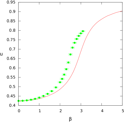
Figure 1: (color online). Dependence on $\beta$ of the solution $u$ of Eq. (43) for $U(2)$ (solid line) and of the $\rho$ expectation value obtained from Monte Carlo simulations (circles).

To perform the mean field study of $U(N)$ models for other values of $N$ one can calculate the Jacobian (32) using numeric integration or the asymptotic expansion (37). In both approaches, we considered several values of $N$, namely $N=2,4,5,8$. The overall picture appears to be qualitatively similar for all $N$: for $\beta$ small, $u$ is almost a constant $u\sim{\cal{O}}(N^{-1})$; when $\beta$ grows, $u$ starts slowly increasing, with the rate of increase reaching its maximum in the region $\beta\sim{\cal{O}}(N^{2})$. When $\beta$ increases further, $u$ continues slowly moving to the value $u=1$ when $\beta\to\infty$. This hints to the fact that the critical point of the $U(N)$ model scales as $N^{2}$, with increasing $N$.

IV Details of numerical simulations

The observables introduced in this work can be related

• to full $U(N)$ and $SU(N)$ spins,

  $$\chi_{u_{N}}(x)\ =\ \rho(x)\ e^{i\omega(x)}\ ,$$ (44)

• or only to their $U(1)$ part,

  $$\chi_{u_{1}}(x)\ =\ e^{i\omega(x)}\ .$$ (45)

The corresponding magnetization is defined as follows:

$$M_{L}^{u}\ =\ \frac{1}{L^{2}}\ \sum_{x}\chi_{u}(x)\ =\ |M_{L}^{u}|e^{i\psi}\ ,$$ (46)

where $u$ can stand either for $u_{N}$ or $u_{1}$. Then, all observables are defined in a standard way:

• Mean absolute magnetization, $\left\langle|M_{L}^{u}|\right\rangle$,

• Magnetization susceptibility,

  $$\chi^{(M_{L})}\ =\ L^{2}(\left\langle|M_{L}^{u}|^{2}\right\rangle-\left\langle|M_{L}^{u}|\right\rangle^{2})\ ,$$ (47)

• Binder cumulants,

  $$U^{(M_{L})}\ =\ 1-\frac{\left\langle|M_{L}^{u}|^{4}\right\rangle}{3\left\langle|M_{L}^{u}|^{2}\right\rangle^{2}}\quad\text{or}\quad B_{4}^{(M_{L})}=\frac{\langle\left|M_{L}^{u}\right|^{4}\rangle}{\langle\left|M_{L}^{u}\right|^{2}\rangle^{2}}\ ,$$ (48)

• Second moment correlation length $\xi_{2}$,

  $$\xi_{2} = \frac{\sqrt{\frac{\chi}{F}-1}}{2\sin{\pi/L}}\ ,$$

  $$\chi = \left\langle\left|\sum_{x,y}\chi_{u}(x,y)\right|^{2}\right\rangle\ ,$$

  $$F = \left\langle\left|\sum_{x,y}e^{2\pi ix/L}\chi_{u}(x,y)\right|^{2}\right\rangle\ .$$ (49)

For the $SU(N)$ model we also introduce the rotated magnetization $M_{R}=|M_{L}^{u_{N}}|\cos{N\psi}$, its mean value and susceptibility.

Simulations for the $U(2)$ model were done using the effective model given in Eq. (23) for $\lambda=0$ and with the exact Jacobian for $U(2)$ model given in Eq. (34). For the update of the $\rho$ variables a heat-bath algorithm was used, while $\omega$ variables were updated using the single-cluster Wolff algorithm described in Wolff (1989). In a typical run, for one choice of the couplings, 50000 measurements were taken, with a whole lattice heat-bath sweep and 10 Wolff cluster updates between two subsequent measurements.

For $SU(N)$ models the original formulation given in Eq. (1) was used. The $SU(N)$ matrices $W(x)$ were parametrized by their eigenvalues $e^{i\omega_{i}}$, since both the partition function of the model and the observables can be defined in terms of these eigenvalues. For updating the $\omega_{i}$ variables the Metropolis algorithm together with the Wolff cluster update using only $Z(N)$ reflections were adopted. We used lattices with size ranging from 8 to 256. In a typical run, for one choice of the couplings, 25000 measurements were taken, with 10 Metropolis updates of the whole lattice (with 20 hits per lattice site) and two Wolff cluster updates between two subsequent measurements.

V BKT transition in $U(2)$ spin model

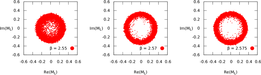
Figure 2: (color online). Scatter plots of the complex magnetization $M_{L}$ at $\beta=2.55,2.57,2.575$ in $U(2)$ on a $512^{2}$ lattice.

In our numerical investigation of the $U(2)$ spin model we proceed in three steps: we first check the existence of a BKT transition to a massless phase, then locate the critical coupling as precisely as possible and, finally, check its universality character via the determination of critical indices.

A clear indication of the two-phase structure is provided by scatter plots of the complex magnetization $M_{L}$ at different values of $\beta$ and for all considered lattice sizes. Increasing $\beta$ we observe a transition from a disordered phase, characterized by a uniform distribution around zero, to a massless phase, characterized by a “ring distribution”. Such observation is reported in Fig. 2 for $L=512$.

The next step is the precise location of the phase transition, i.e. the identification of the critical coupling $\beta_{\rm c}$. To accomplish this task, following Hasenbusch (2005, 2008), we can make use of appropriate fit Ansätze both for the second-moment correlation length and for the Binder cumulant versus the lattice size. The second-moment correlation length and the Binder cumulant, in correspondence to a BKT transition, are indeed found to be RG-invariant quantities and to take universal values that are known for the $XY$ model Hasenbusch (2005, 2008). Also their finite size scaling (FSS) behavior has been studied within the 2D $XY$ model providing us with the following Ansätze:

• for the second-moment correlation length,

  $$\frac{\xi_{2}(\beta,L)}{L}=a(\beta)-\frac{b(\beta)}{\mathrm{ln}(L)+c(\beta)}\;,$$ (50)

  where $a_{\rm c}=a(\beta_{\rm c})=0.7506912\dots$ and $b_{\rm c}=b(\beta_{\rm c})=0.212430\dots$ at the critical point in the $XY$ model;

• for the Binder cumulant,

  $$B_{4}^{(M_{L})}(\beta,L)=a(\beta)-\frac{b(\beta)}{\mathrm{ln}(L)+c(\beta)}+\frac{d(\beta)}{(\mathrm{ln}(L)+c(\beta))^{2}}\;,$$ (51)

  where $a_{\rm c}=a(\beta_{\rm c})=1.018192\dots$ and $b_{\rm c}=b(\beta_{\rm c})=0.017922\dots$ at the critical point in the $XY$ model, and also subleading logarithmic corrections are indicated, since they are found to be important.

To extract the critical point from the scaling of $\xi_{2}$ and $B_{4}^{(M_{L})}$ with the lattice size $L$, the following methods are used:

• at each fixed value of $\beta$ the fit of $\xi_{2}$ and $B_{4}^{(M_{L})}$ data is performed, respectively via the Ansatz in Eq. (50) or Eq. (51), fixing $b(\beta)$ to the known value $b_{\rm c}$. An estimate of $\beta_{\rm c}$ is then given by the $\beta$-value at which $a(\beta)=a_{\rm c}$;

• the same procedure as before, but fixing $a(\beta)=a_{\rm c}$ and extracting $\beta_{\rm c}$ from the requirement that $b(\beta_{\rm c})=b_{\rm c}$.

Our results are illustrated in Fig. 4 and Fig. 4, respectively for the second-moment correlation length and the Binder cumulant $B_{4}$. To be conservative, one can quote $\beta_{\rm c}=2.590\pm 0.005$.

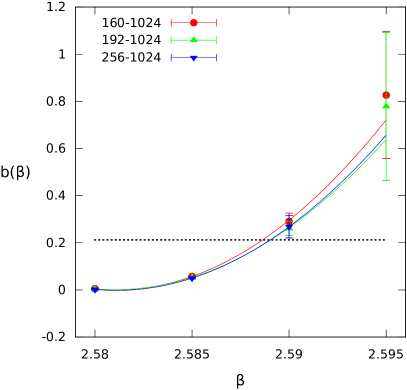
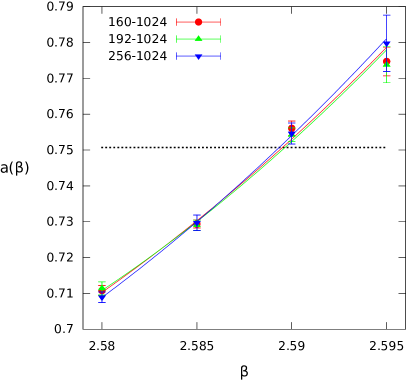
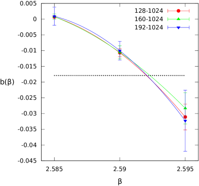
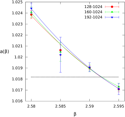
Figure 3: (color online). Determination of $\beta_{\rm c}$ from the second-moment correlation length. (Left) Fit parameter $b(\beta)$ extracted from fits of $\xi_{2}$ via Eq. (50) fixing $a(\beta)$ to the known value $a_{\rm c}=0.7506912$. The horizontal dashed line marks the expected value $b_{\rm c}$. (Right) Fit parameter $a(\beta)$ extracted from fits of $\xi_{2}$ via Eq. (50) fixing $b(\beta)$ to the known value $b_{\rm c}=0.2124300$. The horizontal dashed line marks the expected value $a_{\rm c}$.

Figure 4: (color online). Determination of $\beta_{\rm c}$ from fits of the Binder cumulant $B_{4}$. (Left) Fit parameter $b(\beta)$ extracted from fits of $B_{4}$ via Eq. (51) fixing $a(\beta)$ to the known value $a_{\rm c}=1.018192$. The horizontal dashed line marks the expected value $b_{\rm c}$. (Right) Fit parameter $a(\beta)$ extracted from fits of $B_{4}$ via Eq. (51) fixing $b(\beta)$ to the known value $b_{\rm c}=0.017922$. The horizontal dashed line marks the expected value $a_{\rm c}$.

As a remark about the fitting procedure, one can observe that its stability, with respect to the volumes included in the fit, can be inspected by changing the range of lattice sizes included in the fit and by checking that the extracted fit parameters are compatible within errors once $L$ is large enough. We have found that such a stability in the fits is achieved as soon as the lowest size considered in the fits is $L=128$ for the Binder cumulant and $L=160$ for the second-moment correlation length.

Once the critical coupling has been estimated, we are able to extract critical indices out of the FSS behavior at the critical coupling of :

• the magnetization $|M_{L}|$ that is expected to satisfy the scaling law

  $$|M_{L}|=aL^{-\nicefrac{{\beta}}{{\nu}}}\,\mathrm{ln}^{r}L\;,$$ (52)

• the susceptibility $\chi^{(M_{L})}_{L}$ that is expected to satisfy the scaling law

  $$\chi^{(M_{L})}_{L}=aL^{\nicefrac{{\gamma}}{{\nu}}}\,\mathrm{ln}^{r}L\;.$$ (53)

Results are summarized in Table 2 and Table 2 for the case of magnetization and susceptibility, respectively.

Table 1: Fit parameters $a$, $-\nicefrac{{\beta}}{{\nu}}$, and $r$ obtained from fits of the magnetization via Eq. (52) over the size range $[L_{\mathrm{min}},L_{\mathrm{max}}=1024]$.

$\beta_{\rm c}$	$L_{\mathrm{min}}$	$a$	$-\nicefrac{{\beta}}{{\nu}}$	$r$	$\chi_{r}^{2}$
2.59	64	0.71025 $\pm$ 0.00328	$-$0.12527 $\pm$ 0.00120	0.04307 $\pm$ 0.00659	1.20
2.59	96	0.70055 $\pm$ 0.00286	$-$0.12836 $\pm$ 0.00098	0.06119 $\pm$ 0.00556	0.35
2.59	128	0.70089 $\pm$ 0.00469	$-$0.12826 $\pm$ 0.00151	0.06055 $\pm$ 0.00879	0.42
2.59	160	0.70915 $\pm$ 0.00381	$-$0.12587 $\pm$ 0.00116	0.04596 $\pm$ 0.00690	0.15
2.59	192	0.70738 $\pm$ 0.00575	$-$0.12635 $\pm$ 0.00168	0.04900 $\pm$ 0.01018	0.18
2.59	256	0.70322 $\pm$ 0.01075	$-$0.12746 $\pm$ 0.00299	0.05600 $\pm$ 0.01854	0.24

Table 2: Fit parameters $a$ and $\nicefrac{{\gamma}}{{\nu}}$ obtained from fits of the magnetic susceptibility via Eq. (53) for $r=0$ over the size range $[L_{\mathrm{min}},L_{\mathrm{max}}=1024]$; including logarithmic corrections with $r$ either free or fixed at $r=0.125$ did not improve the fits.

$\beta_{c}$	$L_{\mathrm{min}}$	$a$	$\nicefrac{{\gamma}}{{\nu}}$	$\chi_{r}^{2}$
2.59	160	0.00293 $\pm$ 0.00010	1.73455 $\pm$ 0.00585	2.69
2.59	192	0.00282 $\pm$ 0.00010	1.74060 $\pm$ 0.00581	1.82
2.59	256	0.00273 $\pm$ 0.00013	1.74527 $\pm$ 0.00765	1.87
2.59	384	0.00249 $\pm$ 0.00005	1.75966 $\pm$ 0.00314	0.14
2.59	512	0.00241 $\pm$ 0.00003	1.76431 $\pm$ 0.00180	0.02

VI BKT transition in $SU(N=5,8)$ spin models with adjoint term

It is widely expected that the phase transition in $2D$ $SU(N)$ spin models with only the fundamental representation term is certainly first order for $N>4$. On the other hand, if one adds an adjoint-representation term with its own coupling $\lambda$, in the limit $\lambda\to\infty$ one gets the partition function of $Z(N)$, so there should be two infinite-order phase transitions in this case. It is possible that the phase structure of $2D$ $Z(N)$ spin models is restored already at some finite value of $\lambda$.

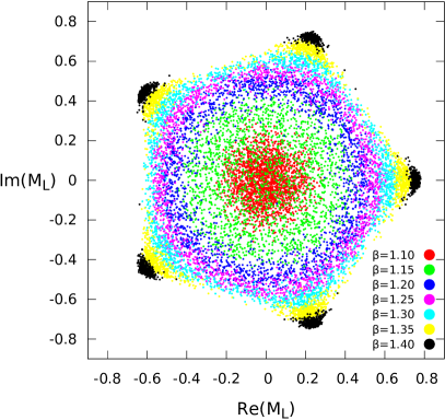
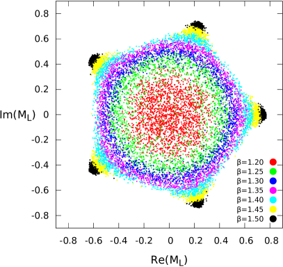
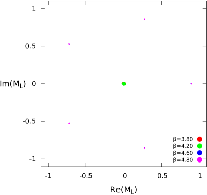
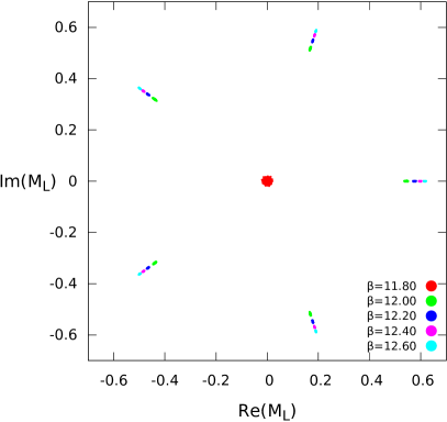
Figure 5: (color online). Scatter plots of the complex magnetization $M_{L}$ in $SU(5)$. (Top-left) $\lambda=1.00$ and $\beta\in[1.10,1.40]$ on a $128^{2}$ lattice. (Top-right) $\lambda=0.80$ and $\beta\in[1.20,1.50]$ on a $128^{2}$ lattice. (Bottom-left) $\lambda=0.75$ and $\beta\in[3.80,4.80]$ on a $32^{2}$ lattice. (Bottom-right) $\lambda=0.00$ and $\beta\in[11.80,12.60]$ on a $128^{2}$ lattice.

To study the phase transitions in $SU(N)$ models, we have performed numerical simulations of $SU(5)$ and $SU(8)$ models. In the $\lambda=0$ case our results are consistent with the existence of a first order phase transition. In particular, we see no intermediate phase with restored $U(1)$ symmetry and the change of the mean magnetization between phases takes place very fast even for small lattice sizes; moreover, around the critical point there are signs of a mixed phase, i.e. the system stays for some time in one phase and then jumps to the other one. This behavior continues for small $\lambda$ values. However, the phase structure of our model is found to significantly depend on the coupling $\lambda$ of the adjoint interaction term: when $\lambda$ becomes large enough, it changes to that of $2D$ $Z(N)$ model, i.e. an intermediate phase with $U(1)$ symmetry appears, which can be seen from the ring-like scatter plot of the complex magnetization (see Figs. 5 and 6). A three-phase structure is then found in this case: from the disordered low-$\beta$ phase, through a massless phase for $\beta_{\rm c}^{(1)}<\beta<\beta_{\rm c}^{(2)}$, to an ordered high-$\beta$ phase. There was no attempt neither to precisely locate the transition, nor to check its universality character.

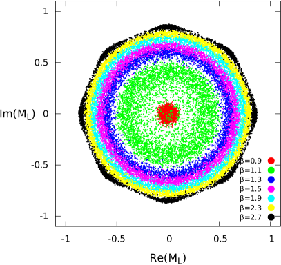
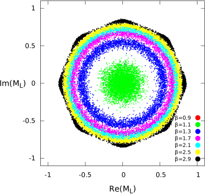
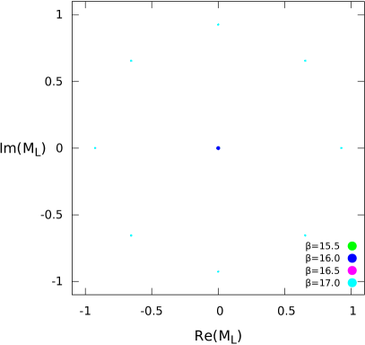
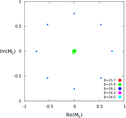
Figure 6: (color online). Scatter plots of the complex magnetization $M_{L}$ in $SU(8)$. (Top-left) $\lambda=2.00$ and $\beta\in[0.90,2.70]$ on a $128^{2}$ lattice. (Top-right) $\lambda=1.10$ and $\beta\in[0.90,2.90]$ on a $128^{2}$ lattice. (Bottom-left) $\lambda=0.90$ and $\beta\in[15.50,17.00]$ on a $64^{2}$ lattice. (Bottom-right) $\lambda=0.00$ and $\beta\in[25.70,26.50]$ on a $128^{2}$ lattice.

Beyond the scatter plots, further information about the nature of the observed transitions is provided by the behavior with $\beta$, and for various fixed $\lambda$ values, of the ordinary and rotated magnetization and their susceptibilities (Fig. 7 and Fig. 8).

A remark is in order about the necessity to introduce and measure the rotated magnetization: what we need is a quantity that is sensitive to the difference in the magnetization distribution between the massless and ordered phase. However the two phases differ only for the angular structure of the complex magnetization, hence the susceptibility and even the Binder cumulant for the ordinary magnetization are not able to detect the massless to ordered transition. The rotated magnetization, instead, yields a finite value when there is a non-trivial angular structure, while it vanishes when $\psi$ is isotropically distributed. From the peaks of the susceptibilities of both ordinary and rotated magnetization we are able to infer the approximate location of the critical points.

The dependence of critical points on $\lambda$ also changes with the kind of transition: for small $\lambda$, when the first order phase transition takes place, $\beta_{\rm c}$ decreases almost linearly with $\lambda$; but once we get to the two infinite-order transitions, the critical points $\beta_{\rm c}^{(1)}$ and $\beta_{\rm c}^{(2)}$ appear at much lower values than the ones for $\beta_{\rm c}$ observed during this linear decrease. Whether this means that the transition point starts to decrease faster in the vicinity of the critical $\lambda$ or that the transition lines are disjoint, remains unclear and requires a more refined study. It is important, however, to note that, when $\lambda$ further grows, the two transition points converge to those of the corresponding $Z(N)$ model. However, we have currently not yet achieved a precise numerical estimate of the minimal $\lambda$ values at which BKT transitions manifest themselves in these models.

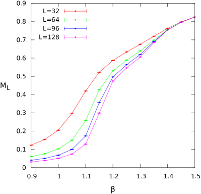
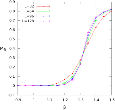
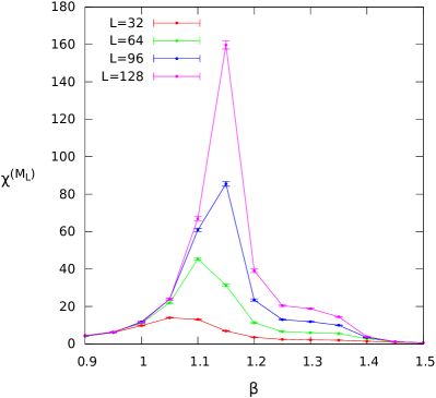
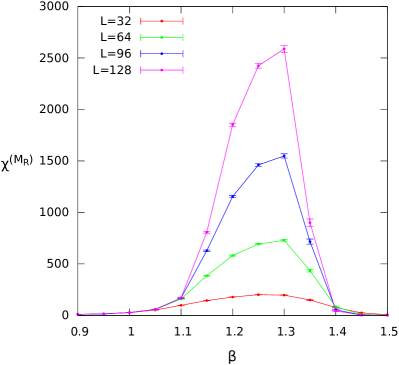
Figure 7: (color online). Magnetization (top-left), its susceptibility (bottom-left), rotated magnetization (top-right) and its susceptibility (bottom-right) versus $\beta$ in the $SU(5)$ spin model for $\lambda=1.0$.

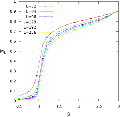
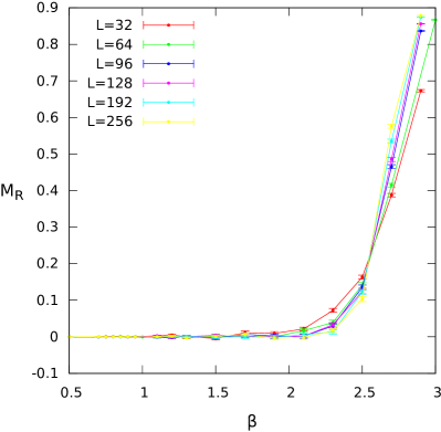
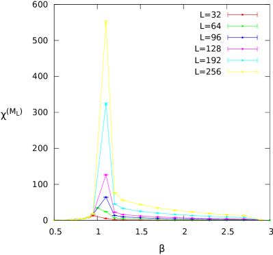
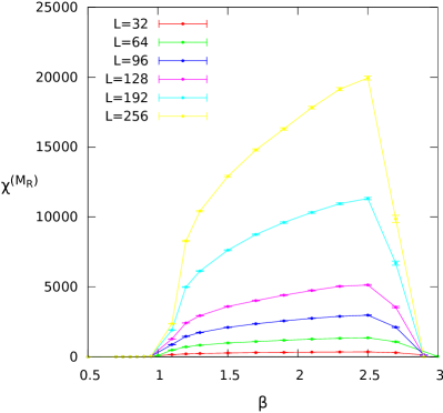
Figure 8: (color online). Magnetization (top-left), its susceptibility (bottom-left), rotated magnetization (top-right) and its susceptibility (bottom-right) versus $\beta$ in the $SU(8)$ spin model for $\lambda=2.0$.

VII Summary and Discussion

The BKT phase transition occurs in various two-dimensional spin and three-dimensional finite-temperature gauge models. All these models have one feature in common: they are Abelian models. To the best of our knowledge, this type of phase transition has not been observed in any non-Abelian model.

In this paper we have investigated $U(N)$ and $SU(N)$ spin models in two dimensions with the goal of finding evidences for the existence of such phase transition. Our findings can be shortly summarized as follows:

• We presented simple arguments, based on the symmetry and on Berezinskii-like calculations, that the two-point correlation function in $2D$ $U(N)$ models decays with power-law at large $\beta$. Since the correlation function has an exponential decay in the strong coupling region, this may indicate, similarly to the $XY$ model, a very smooth transition from the massive to the massless phase.

• More quantitative arguments in a favor of BKT transition have been obtained within the effective dual model (28). A combination of the mean field and RG analysis led to the conclusion that $U(N)$ models belong to the universality class of the $XY$ model.

• To verify the above scenario we performed detailed numerical simulations of the $U(2)$ model. We have located the critical point of the phase transition and computed some critical indices, which appear to agree with those of the $XY$ model.

• In the case of $SU(N)$ models we have considered a mixed fundamental-adjoint action, with two independent coupling constants. When the adjoint coupling is small, our numerical results reveal the existence of a first order phase transition. When the adjoint coupling grows, the fluctuations of $SU(N)$ variables are suppressed and the leading contribution comes from the center subgroup. Under such circumstances, one could expect that the phase structure is similar to that of the $2D$ $Z(N)$ model. Indeed, numerical investigations of $SU(N=5,8)$ support the existence of two BKT-like phase transitions above a certain critical value of the adjoint coupling.

To clarify completely the physical picture of the phase transitions in these models one should still solve some open issues. Among them is the extension of the analytical arguments to $SU(N)$ models. This can be done with the help of the dual formulation (III.2). Then, to establish the universality class of $SU(N)$ models and to compute the corresponding critical indices, we need to perform large-scale numerical simulations of these models. The work on these and some other problems is in progress.

Finally, we would like to stress again that the models studied here can be regarded as the simplest ones describing the interaction between Polyakov loops in the strong coupling limit of a $3D$ LGT at finite temperature. It is well known that in the case of the $SU(N)$ LGT one expects a first order phase transition if $N$ is large enough Liddle and Teper (2008). Indeed, our results for $N=5,8$, and in the region of small adjoint coupling $\lambda$, agree with this conclusion. Of course, the higher-order corrections to the effective Polyakov loop model generate all irreducible representations of the group, including the adjoint one. At the present stage we can only speculate that the values of the corresponding adjoint couplings are rather small and lay below the critical $\lambda$ at which the BKT transition occurs. In order to get the BKT transition in gauge models, one should add to the Wilson action in the fundamental representation the adjoint term. This is an intriguing possibility which deserves a further investigation.

References

- Berezinskii (1971) V. Berezinskii, JETP 32, 493 (1971).
- Kosterlitz and Thouless (1973) J. M. Kosterlitz and D. J. Thouless, J. Phys. C6, 1181 (1973).
- Kosterlitz (1974) J. M. Kosterlitz, J. Phys. C7, 1046 (1974).
- Frohlich and Spencer (1981) J. Frohlich and T. Spencer, Commun. Math. Phys. 81, 527 (1981).
- Elitzur et al. (1979) S. Elitzur, R. B. Pearson, and J. Shigemitsu, Phys. Rev. D19, 3698 (1979).
- Einhorn et al. (1980) M. B. Einhorn, R. Savit, and E. Rabinovici, Nucl. Phys. B170, 16 (1980).
- Hamer and Kogut (1980) C. J. Hamer and J. B. Kogut, Phys. Rev. B 22, 3378 (1980).
- Nienhuis (1984) B. Nienhuis, J. Statist. Phys. 34, 731 (1984).
- Kadanoff (1978) L. P. Kadanoff, J. Phys. A11, 1399 (1978).
- Cardy and Sugar (1980) J. L. Cardy and R. L. Sugar, J. Phys. A13, L423 (1980).
- Domany et al. (1980) E. Domany, D. Mukamel, and A. Schwimmer, Journal of Physics A: Mathematical and General 13, L311 (1980).
- Tomita and Okabe (2002) Y. Tomita and Y. Okabe, Phys. Rev. B 65, 184405 (2002).
- Baek and Minnhagen (2010) S. K. Baek and P. Minnhagen, Phys. Rev. E 82, 031102 (2010).
- Borisenko et al. (2011) O. Borisenko, G. Cortese, R. Fiore, M. Gravina, and A. Papa, Phys. Rev. E83, 041120 (2011), arXiv:1011.5806 [hep-lat] .
- Borisenko et al. (2012a) O. Borisenko, V. Chelnokov, G. Cortese, R. Fiore, M. Gravina, and A. Papa, Phys. Rev. E85, 021114 (2012a), arXiv:1112.3604 [hep-lat] .
- Parga (1981) N. Parga, Phys. Lett. B107, 442 (1981).
- Svetitsky and Yaffe (1982) B. Svetitsky and L. G. Yaffe, Nucl. Phys. B210, 423 (1982).
- Borisenko et al. (2008) O. Borisenko, M. Gravina, and A. Papa, J. Stat. Mech. 0808, P08009 (2008), arXiv:0806.2081 [hep-lat] .
- Borisenko et al. (2010) O. Borisenko, R. Fiore, M. Gravina, and A. Papa, J. Stat. Mech. 1004, P04015 (2010), arXiv:1001.4979 [hep-lat] .
- Borisenko (2007) O. Borisenko, PoS LAT2007, 170 (2007).
- Borisenko and Chelnokov (2014) O. Borisenko and V. Chelnokov, Phys. Lett. B730, 226 (2014), arXiv:1311.2179 [hep-lat] .
- Borisenko et al. (2015) O. Borisenko, V. Chelnokov, M. Gravina, and A. Papa, JHEP 09, 062 (2015), arXiv:1507.00833 [hep-lat] .
- Borisenko et al. (2012b) O. Borisenko, V. Chelnokov, G. Cortese, R. Fiore, M. Gravina, A. Papa, and I. Surzhikov, Phys. Rev. E86, 051131 (2012b), arXiv:1206.5607 [hep-lat] .
- Borisenko et al. (2013) O. Borisenko, V. Chelnokov, G. Cortese, M. Gravina, A. Papa, and I. Surzhikov, Nucl. Phys. B870, 159 (2013), arXiv:1212.3198 [hep-lat] .
- Borisenko et al. (2014a) O. Borisenko, V. Chelnokov, G. Cortese, M. Gravina, A. Papa, and I. Surzhikov, Nucl. Phys. B879, 80 (2014a), arXiv:1310.5997 [hep-lat] .
- Borisenko et al. (2014b) O. Borisenko, V. Chelnokov, M. Gravina, and A. Papa, Nucl. Phys. B888, 52 (2014b), arXiv:1408.2780 [hep-lat] .
- Feldman (1999) D. E. Feldman, Journal of Experimental and Theoretical Physics Letters 70, 135 (1999).
- Feldman (2001) D. E. Feldman, International Journal of Modern Physics B 15, 2945 (2001).
- Patrascioiu and Seiler (1995) A. Patrascioiu and E. Seiler, Phys. Rev. Lett. 74, 1920 (1995).
- Mermin and Wagner (1966) N. D. Mermin and H. Wagner, Phys. Rev. Lett. 17, 1133 (1966).
- Liddle and Teper (2008) J. Liddle and M. Teper, (2008), arXiv:0803.2128 [hep-lat] .
- Wolff (1989) U. Wolff, Phys. Rev. Lett. 62, 361 (1989).
- Hasenbusch (2005) M. Hasenbusch, J. Phys. A38, 5869 (2005), arXiv:cond-mat/0502556 [cond-mat] .
- Hasenbusch (2008) M. Hasenbusch, Journal of Statistical Mechanics: Theory and Experiment 2008, P08003 (2008).
- Note (1) The symbol here denotes a critical index and not, as before, the coupling of the theory.