Origin of Confining Force

Abstract

In this article we present exact calculations that substantiate a clear picture relating the confining force of QCD to the zero-modes of the Faddeev-Popov (FP) operator $\mathcal{M}(gA)=-\partial\cdot D(gA)$. This is done in two steps. First we calculate the spectral decomposition of the FP operator and show that the ghost propagator $\mathcal{G}(k;gA)=\langle\vec{k}|\mathcal{M}^{-1}(gA)|\vec{k}\rangle$ in an external gauge potential $A$ is enhanced at low $k$ in Fourier space for configurations $A$ on the Gribov horizon. This results from the new formula in the low-$k$ regime $\mathcal{G}^{ab}(k,gA)=\delta^{ab}\lambda_{|\vec{k}|}^{-1}(gA)$, where $\lambda_{|\vec{k}|}(gA)$ is the eigenvalue of the FP operator that emerges from $\lambda_{|\vec{k}|}(0)=\vec{k}^{2}$ at $A$ = 0. Next we derive a strict inequality signaling the divergence of the color-Coulomb potential at low momentum $k$ namely, $\widetilde{\mathcal{V}}(k)\geq k^{2}\mathcal{G}^{2}(k)$ for $k\to 0$, where $\widetilde{\mathcal{V}}(k)$ is the Fourier transform of the color-Coulomb potential $\mathcal{V}(r)$ and $\mathcal{G}(k)$ is the ghost propagator in momentum space. Although the color-Coulomb potential is a gauge-dependent quantity, we recall that it is bounded below by the gauge-invariant Wilson potential, and thus its long range provides a necessary condition for confinement. The first result holds in the Landau and Coulomb gauges, whereas the second holds in the Coulomb gauge only.

I Introduction

Experimentally, color confinement is the most well tested phenomenon of QCD - verified every time a free quark from a high energy collision doesn’t make it to the calorimeters without bounding itself up into hadrons. Nevertheless, theoretically we lack a satisfying mechanism to reveal this feature. This is not to say our theory of strong interactions is incapable of describing confinement. When the QCD partition function is simulated on a spacetime lattice, gauge-invariant observables can be computed, revealing a confining gluonic flux tube between colored states. These simulations reveal a picture of a string with a tension (energy per length) that to leading order yields a linearly rising potential asymptotically at long distances. An analytic method that could show the origin of this confining force has long been sought after by generations of field theorists.

Understanding the origin of forces between particles in QCD is significantly more challenging than its abelian cousin because quantities that were once gauge invariant like the curvature of the gauge connection, are now gauge covariant. Thus, even the color-electric field is a gauge-dependent quantity so the naive notion of “force” that one might have in QCD which would follow from a non-abelian Lorentz force law is more subtle. This is a situation much like gravity, where observables that were once gauge invariant (local scalar fields) become gauge covariant with respect to diffeomorphisms. The root of this complication is that in non-abelian theories, the kinetic terms introduce non-linear interactions between the force carriers themselves, and thus the color-electric field itself carries charge.

The first crucial result that we make use of in this article, allowing one to extract gauge-invariant information from a gauge dependent quantity, is the theorem “no confinement without Coulomb confinement” from Zwanziger (2003). This theorem tells us that a necessary condition for confinement is that the color-Coulomb potential $\mathcal{V}(r)$ be confining via the inequality

$$V_{W}(r)<-C\mathcal{V}(r)\;\;\;r\to\infty,$$ (1)

where $V_{W}(r)$ is the Wilson potential, ie the contribution to the energy coming from the flux tube formed between two quarks that furnish some representation with Casimir $C$.

$\mathcal{V}(\vec{x})$ is defined to be the instantaneous part of the time-time component of the gluon propagator in Coulomb gauge Cucchieri and Zwanziger (2001)

$$\langle A_{0}^{a}(x)A_{0}^{b}(y)\rangle=\delta^{ab}[\mathcal{V}(\vec{x}-\vec{y})\delta(x_{0}-y_{0})-P(x-y)],$$ (2)

where $P(x-y)$ is non-instantaneous. This formula is obtained via the first-order formalism in Coulomb gauge Baulieu and Zwanziger (1999). After integrating out $A_{0}$ and the longitudinal component of the conjugate momentum, $\pi_{i}$, and resolving Gausses law, the partition function becomes

$$Z(J_{0})=\int\mathcal{D}\pi^{\mathrm{tr}}_{i}\mathcal{D}A^{\mathrm{tr}}_{i}\mathrm{exp}\left[\int d^{D}x\left(i\pi^{\mathrm{tr}}_{i}\dot{A}_{i}^{\mathrm{tr}}-\frac{1}{2}(\pi^{\mathrm{tr}}_{i})^{2}-\frac{1}{2}B_{i}^{2}-\frac{1}{2}\rho\left({\mathcal{M}}^{-1}(-\partial)^{2}{\mathcal{M}}^{-1}\rho\right)\right)\right]$$ (3)

with the color-charge density $\rho$ given by

$$\rho=\rho_{0}+\rho_{dyn}=J_{0}^{a}+gf^{abc}A_{i}^{b\,\mathrm{tr}}\pi_{i}^{c\,\mathrm{tr}},$$ (4)

the superscript $\mathrm{tr}$ indicates a transverse 3-vector, and $B_{i}$ is the color-magnetic field. Here $({\mathcal{M}}^{-1})^{ab}(\vec{x},\vec{y};gA)$ is the ghost propagator in Coulomb gauge in a transverse background potential $A_{i}^{b}$, with $\partial_{i}A_{i}^{b}=0$,

$$\mathcal{M}^{ac}\equiv-D^{ac}\cdot\partial=\mathcal{M}_{0}^{ac}+\mathcal{M}_{1}^{ac}=(-\partial^{2})\delta^{ac}-gf^{abc}A_{i}^{b}\partial_{i}$$ (5)

is the Faddeev-Popov operator in a space of dimension $d$, where $A_{i}$ is transverse $\partial_{i}A_{i}=0$, so $\mathcal{M}$ is hermitian, and $i=1,...d$. The indices $a,b,c=1,...N^{2}-1$ take values in the adjoint representation of the $SU(N)$ color group. In Coulomb gauge $d=3$ is the dimension of the ordinary 3-dimensional space part of 4-dimensional Euclidean or Minkowskian space. Those of our results which concern the ghost propagator, hold also in Landau gauge, in which case $d$ is the dimension of Euclidean space-time. By taking variational derivatives of $Z(J_{0})$ and setting $J_{0}=0$, we get

$$\delta^{ab}\mathcal{V}(\vec{x}-\vec{y})=\left<(\mathcal{N}^{-1})_{\vec{x}\vec{y}}^{ab}\right>$$ (6)

and

$$\delta^{ab}P(x-y)=\left<(\mathcal{N}^{-1}\rho_{dyn})_{x}^{a}(\mathcal{N}^{-1}\rho_{dyn})_{y}^{b}\right>$$ (7)

where

$$\mathcal{N}^{-1}=\mathcal{M}^{-1}(-\partial^{2})\ \mathcal{M}^{-1}.$$ (8)

The quantity $({\mathcal{N}}^{-1})^{ab}(\vec{x},\vec{y};gA)$ is the color-Coulomb potential in a transverse background potential $A_{i}^{b}$. To all orders in perturbation theory $g^{2}\mathcal{V}(\vec{x}-\vec{y})$ is a renormalization-group invariant Zwanziger (1998). That is, the color-Coulomb interaction energy, $g^{2}\mathcal{V}(\vec{x}-\vec{y})$, is scheme-independent, and if this is also true non-perturbatively than $g^{2}\mathcal{V}(\vec{x}-\vec{y})$ has a well defined value in Joules at any given separation $|\vec{x}-\vec{y}|$ in meters.

An important point is that both the instantaneous part $\mathcal{V}(\vec{x}-\vec{y})$ and the non-instantaneous part $P(x-y)$ are each the kernel of a positive operator, so the opposite signs in (2) mean that $P(x-y)$ is screening while $\mathcal{V}(\vec{x}-\vec{y})$ is anti-screening. Which one dominates is a dynamical question that we will not address here. However while a sufficient condition for confinement is the ideal, one can at least obtain a necessary condition by calculating the infrared behavior of the two-point instantaneous correlator $\mathcal{V}(\vec{x})$ which is the anti-screening part.

In this article we show by direct calculation that $\mathcal{V}(\vec{x}-\vec{y})$ is in fact confining, granted a few not unreasonable assumptions about certain generic features of the spectrum of the Faddeev Popov (FP) operator. An important tool in this analysis is the implementation of the non-local ‘horizon condition’ Zwanziger (1989) which restricts the gluon measure to the first Gribov region Gribov (1978). It should come as no surprise that the Gribov ambiguity (which is the statement that no continuous, finite-energy, globally defined gauge connection exists over spacetime) has a role to play in the long distance behavior of YM theory. In Singer (1978) Singer showed that this problem is a logical consequence of the highly non-trivial topology of the space of connections over spacetime quotiented by the group action of any non-abelian group. Since this obstruction is topological, perturbation theory in a neighborhood of a flat connection is unaffected and thus the ambiguity is relegated to a merely academic discussion in most textbooks on field theory which mostly seek perturbative treatments of QCD. To probe very large length scales of the gluon field however, we must concern ourselves with a global section of the SU(3) principle fibre bundle over spacetime, and thus the non-trivial topology of the bundle can be felt. Indeed it was shown immediately in Gribov’s founding paper Gribov (1978) that this in fact happens. In ameliorating this ambiguity, the low $k$ modes of the gluon propagator go from IR singular to IR suppressed, and the pole is removed from the real axis, thus removing the gluon from the physical spectrum. With the gluon suppressed, in the Gribov confinement scenario, it’s the enhancement of the ghost propagator that is intuited as responsible for the long-range force.

Other scenarios also relate this treatment of the Gribov ambiguity to confinement. A recent, very elegant picture was provided by Reinhardt in Reinhardt (2008) to show that the ‘no-pole’ condition, an equivalent statement to the aforementioned ‘horizon condtion’, implies that the QCD vacuum is a perfect color dielectric ($\epsilon(k)=0$) resulting in a dual Meissner effect, confining electric flux into vortices, which due to dynamical quark pair creation can never be macroscopic in size.

Our approach will be to realize the concrete connection between the horizon condition and the divergence of the color-Coulomb potential (CCP). This is done by using scattering theory techniques to locate the Gribov horizon. We will also use these results to prove a specific asymptotic relationship between a lower bound for the CCP and the ghost propagator, namely

$$\widetilde{\mathcal{V}}(k)\geq k^{2}\mathcal{G}^{2}(k)\ \ \ \ \ \ {\rm for}\ k\to 0,$$ (9)

where $\widetilde{\mathcal{V}}(k)$ is the Fourier transform of the color-Coulomb potential $\mathcal{V}(r)$, and $\mathcal{G}(k)$ is the ghost propagator in momentum space. This makes explicit the role of the enhanced ghost propagator in confinement. Since $\mathcal{V}(\vec{x}-\vec{y})$ is gauge-dependent, this result is not a proof of confinement and, in fact, the non-instantaneous force $P(x)$ in (2) may compensate the instantaneous force, as happens in the deconfinement transition of the gluon plasma at sufficiently high temperature, or when dynamical quarks screen external quarks. However it reverses the question of confinement. The problem now is not to show that a confining force exists; that is always provided by the instantaneous color-Coulomb force. The problem is to determine whether or not this force is compensated by non-instantaneous forces. This provides a very intuitive theory of confinement, quite analogous to our theory of atoms or molecules which are themselves neutral, but are held together by instantaneous Coulomb forces between electrically charged constituents. In this article we have ignored the presence of dynamical quarks because we do not expect that they will screen the color-Coulomb confining force. Indeed we expect that although dynamical quarks do screen the gauge-invariant Wilson potential nevertheless, in the picture provided by the Coulomb gauge, the color-Coulomb potential always acts between elementary color-charges — be they quarks or gluons — just as the electro-static Coulomb potential always acts between elementary electric charges. Indeed it is the presence of the color-Coulomb potential that makes it energetically favorable for color-neutral particles to be formed.

In the final sections, we’ll discuss what can be said about the gauge-invariant aspects of this analysis. We’ll also see how our simple picture holds up next to recent lattice studies of the relevant parts of the FP spectrum.

II The Spectral Decomposition of the FP operator: Results

Gribov showed that covariant gauges weren’t sufficient to fix the gauge redundancy of the measure of the gluon field, and proposed a simple but drastic reduction of the gluon measure of integration. The geometric picture is that the gauge is simply the condition that the gluon field be a critical point, $\delta F=0$, of the functional given by the $L^{2}$ norm,

$$F(A)=\int d^{d}x|A(x)|^{2},$$ (10)

where the variation is done with respect to an infinitesimal gauge transformation. With this condition alone, every local minimum, maximum and saddle point of the same gauge orbit would be redundantly counted in the path integral. Gribov proposed that the first thing one can do to ameliorate this situation is demand that $A(x)$ be such that the FP operator be positive definite. It can be shown that this is equivalent to demanding that $A(x)$ be a local minimum of (10) Maskawa and Nakajima (1978); Zwanziger (1982a); Semenov-Tyan-Shanskii and Franke (1986). Since the inverse of the FP operator is the ghost propagator, Gribov did a semiclassical computation to see where the ghost propagator went through zero away from the usual pole at $k=0$ to derive a condition where the path integration should be cut off in configuration space. This cut-off has been shown to restrict the region of integration to a bounded convex region Zwanziger (1982b); Semenov-Tyan-Shanskii and Franke (1986), and the way it alters perturbation theory already starts to show qualitative features of confinement. This approach to restricting the measure has been followed up by various other methods Vandersickel and Zwanziger (2012) that have lead to a local, renormalizable Lagrangian with spontaneously broken BRST invariance including new auxillary ghosts to implement this cutoff Zwanziger (1989).

In Appendix A, we carefully revisit the heuristic approach to deriving the non-local ‘horizon condition’ which implements the cut off to the Gribov region, found in Zwanziger (1989) using a method akin to degenerate perturbation theory, but does not rely on any perturbative expansion. The idea is that the FP operator can be considered as a deformation of the Laplacian, which is already positive definite. One slowly turns on $gA$ until one of the eigenvalues becomes negative. It should be noted that this will be the way we generate an implicit equation for the eigenvalues, and that at no point do we require $gA$ to be small as in typical perturbation theory. We do however limit our results to asymptotically small $k$ since it’s the infrared region in which we’re interested. We designate by $\lambda_{|\vec{k}|}(gA)$ the eigenvalue of the FP operator coming out of the eigenvalue of $\mathcal{M}_{0}$ at $k^{2}$ as we adiabatically turn on the perturbation $\mathcal{M}_{1}(gA)$.

The details are carried out in Appendices A, B, and C. Here we’ll just present an abridged summary of the results so the reader can continue on to the physics. The eigenvalue of the FP operator for a given connection near $k=0$ in Fourier space is given by

$$\lambda_{|\vec{k}|}(gA)=\vec{k}^{2}\left(1-[(N^{2}-1)dV]^{-1}H(gA)+j_{|\vec{k}|}(gA)\right),$$ (11)

where $j_{|\vec{k}|}(gA)$ vanishes as $k$ tends to $0$. $H(gA)$ is the horizon function given by

$$H(gA)=\int d^{d}x\,d^{d}yD_{i\vec{x}}^{ac}D_{i\vec{y}}^{ae}\left(M^{-1}\right)^{ce}_{\vec{x},\vec{y}}.$$ (12)

The horizon condition Vandersickel and Zwanziger (2012) and no-pole condition Gribov (1978) both yield

$$\left<H(gA)\right>=(N^{2}-1)dV.$$ (13)

This condition enhances the ghost propagator $\mathcal{G}(k)$ at momentum $k=0$. We define a new IR exponent $\eta$ as an ansatz for the behavior of the ensemble average, $\left<\lambda^{-1}_{k}\right>$, which goes to zero like $1/k^{2+\eta}$. As we’ll see, much of the qualitative features of confinement boil down to the value of this exponent. It can be calculated numerically on the lattice and attempts at calculating it analytically make up a large part of the focus of recent studies of long-range QCD using Schwinger Dyson Equations (SDE) and variational methods .

Another important result, is that while to order $k^{2}$ the eigenvalues are strongly perturbed, the projector onto eigenstates of the FP operator adiabatically emerging from the degenerate level $|\vec{k}|$ of the Laplacian remains equal to the unperturbed projector. Namely $P_{|\vec{k}|}(gA)=P_{|\vec{k}|}(0)+O(\vec{k}^{2})$ or in terms of the eigenstates of the FP operator

$$\lim_{\vec{k}\to 0}\sum_{\ \vec{k};|\vec{k}|}|\psi_{\vec{k}}(gA)\rangle\langle\psi_{\vec{k}}(gA)|=\sum_{\ \vec{k};|\vec{k}|}|\vec{k}\rangle\langle\vec{k}|.$$ (14)

(Here and below $\sum_{\ \vec{k};|\vec{k}|}$ means sum on all vectors $\vec{k}=(2\pi\vec{n}/L)$, with the same fixed $|\vec{k}|$, where the $n_{i}$ are integers.) By relating the enhanced ghost propagator $\mathcal{G}(k)$ and the CCP $\widetilde{\mathcal{V}}(k)$ to eigenvalues and projectors onto the space of eigenvectors of the FP operator, we obtain the lower bound (43) on the IR strength of the CCP.

III The Long Range Color Coloumb Potential

In Coulomb gauge the propagator of the Faddeev-Popov ghost is instantaneous,

$$\langle c^{a}(x)\bar{c}^{b}(y)\rangle=\delta^{ab}\mathcal{G}(\vec{x}-\vec{y})\delta(x_{0}-y_{0}),$$ (15)

and is expressed in terms of the Faddeev-Popov operator by

$$\delta^{ab}\mathcal{G}(\vec{x}-\vec{y})=\langle({\mathcal{M}}^{-1})^{ab}(\vec{x},\vec{y};gA)\rangle.$$ (16)

The two operators $\mathcal{M}$ and $\mathcal{N}$ are related by Feuchter and Reinhardt (2004)

$$\mathcal{N}^{-1}=(g\partial_{g}+1){\mathcal{M}}^{-1},$$ (17)

where $\partial_{g}\equiv\partial/\partial g$. This follows from the elementary identity

$$g\partial_{g}{\mathcal{M}}^{-1}=-{\mathcal{M}}^{-1}{\mathcal{M}}_{1}{\mathcal{M}}^{-1}={\mathcal{M}}^{-1}({\mathcal{M}}_{0}-\mathcal{M}){\mathcal{M}}^{-1}=\mathcal{N}^{-1}-\mathcal{M}^{-1}.$$ (18)

The spectral decomposition of the ghost propagator is given by

$$\left(\mathcal{M}^{-1}\right)_{xy}^{ab}=\sum_{n}{\psi_{nx}^{a}\psi_{ny}^{b}\over\lambda_{n}},$$ (19)

where we have used the fact that the Faddeev-Popov operator $\mathcal{M}$ is a real symmetric operator, and we have chosen eigenfunctions, $\mathcal{M}\psi_{n}=\lambda_{n}\psi_{n}$, that are real $\psi_{nx}^{a}=(\psi_{nx}^{a})^{*}$. From (17) we obtain

$$\left(\mathcal{N}^{-1}\right)_{xy}^{ab}=\sum_{n}\left[\left({-g\partial_{g}\lambda_{n}\over\lambda_{n}^{2}}+{1\over\lambda_{n}}\right)\psi_{nx}^{a}\psi_{ny}^{b}+{1\over\lambda_{n}}g\partial_{g}(\psi_{nx}^{a}\psi_{ny}^{b})\right].$$ (20)

We expand $g\partial_{g}\psi_{nx}^{a}=\sum_{m}c_{nm}\psi_{mx}^{a}$, and observe that

$$g\partial_{g}\int d^{d}x\ \psi_{nx}^{a}\psi_{nx}^{a}=2\int d^{d}x\sum_{m}c_{nm}\psi_{mx}^{a}\psi_{nx}^{a}=2c_{nn}=0\hskip 56.9055pt{\rm(no\ sum\ on\ }n),$$ (21)

which vanishes because the eigenfunctions are normalized, $\int d^{d}x\psi_{nx}^{a}\psi_{nx}^{a}=1$. Thus the color-Coulomb potential $\mathcal{N}^{-1}$ in the background field $A_{i}^{a}$ has a kind of spectral decomposition in terms of the eigenfunctions of the Faddeev-Popov operator,

$$\left(\mathcal{N}^{-1}\right)_{xy}^{ab}=\sum_{n}\left({-g\partial_{g}\lambda_{n}\over\lambda_{n}^{2}}+{1\over\lambda_{n}}\right)\psi_{nx}^{a}\psi_{ny}^{b}+\sum_{n\neq m}\left({c_{nm}\over\lambda_{n}}+{c_{mn}\over\lambda_{m}}\right)\psi_{mx}^{a}\psi_{ny}^{b}.$$ (22)

Its trace,

$$\int d^{d}x\left(\mathcal{N}^{-1}\right)_{xx}^{aa}=\sum_{n}\left({-g\partial_{g}\lambda_{n}\over\lambda_{n}^{2}}+{1\over\lambda_{n}}\right),$$ (23)

is expressed in terms of the eigenvalues $\lambda_{n}$ of the Faddeev-Popov operator $\mathcal{M}$.

IV Necessary condition for confining potential

The color-Coulomb potential $\mathcal{V}(\vec{x}-\vec{y})$ is said to be confining if the infrared contribution to the color-Coulomb self-energy $\mathcal{V}(0)$ of any colored particle is divergent Greensite et al. (2004a). This is a necessary condition for physical confinement because of the theorem “no confinement without Coulomb confinement,” Zwanziger (2003) which provides a lower bound on the color-Coulomb potential at large separation. However it is not a sufficient condition.

The color-Coulomb self-energy is given by

$$\mathcal{V}(0) = (N^{2}-1)^{-1}\left\langle(\mathcal{N}^{-1})^{aa}(\vec{x},\vec{x};gA)\right\rangle$$ (24)

$$= [(N^{2}-1)V]^{-1}\left\langle\int d^{d}x\ (\mathcal{N}^{-1})^{aa}(\vec{x},\vec{x};gA)\right\rangle.$$

Since this quantity is a trace it can be expressed in any basis. Thus, from (22), we obtain

$$\mathcal{V}(0)={1\over(N^{2}-1)V}\sum_{|\vec{k}|<k_{\rm max}}\left\langle{-g\partial_{g}\lambda_{|\vec{k}|}(gA)\over\lambda_{|\vec{k}|}^{2}(gA)}+{1\over\lambda_{|\vec{k}|}(gA)}\right\rangle.$$ (25)

We have introduced a cut-off $k_{\mathrm{max}}$ to avoid the ultraviolet divergence of the self-energy. It is the infrared divergence of the self-energy that is a necessary condition for a confining potential. Here $\mathcal{V}(0)$ is expressed entirely in terms of the eigenvalues $\lambda_{|\vec{k}|}(gA)$ of the Faddeev-Popov operator. Whether or not $\mathcal{V}(0)$ is confining is determined by the eigenvalues and the density of eigenvalues in the limit $\vec{k}\to 0$, that is to say by the zero modes.

V Zero modes of Faddeev-Popov operator and confinement

The near-zero eigenvalues of the Faddeev-Popov operator are studied in Appendices A and B. According to (11), the eigenvalues are given to order $\vec{k}^{2}$ by

$$\lambda_{|\vec{k}|}(gA)=\vec{k}^{2}\left(1-[d(N^{2}-1)V]^{-1}H(gA)\right).$$ (26)

The crucial observation is that, to leading order in $\vec{k}$, all eigenvalues $\lambda_{|\vec{k}|}(gA)$, for different $\vec{k}=2\pi\vec{n}/L$, where the $n_{i}$ are integers, pass through zero together in a massive level crossing, at a common Gribov horizon as the result of (13). This is illustrated in Figs. 1 and 2. This massive level crossing also occurs in lattice gauge theory on large lattices as was noted in Zwanziger (1992) under the heading “all horizons are one horizon”.

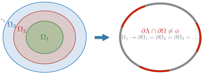
Figure 1: In light of this result, to lowest order in $k$, all levels cross the horizon at once, thus altering the traditional picture of the various Gribov regions to one that makes apparent this infinite density of states. $\Lambda$ is the fundamental modular region which corresponds to the absolute minimum of the functional (10).

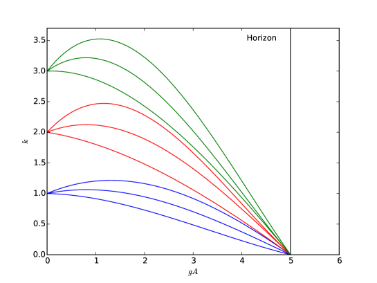
Figure 2: Above is a cartoon (a 1D projection of an infinite dimensional space) of the cubic symmetry degeneracy of the eigenvalues of the finite volume Laplacian being lifted by a perturbation and heading towards zero. Wave vectors are measured in units of $2\pi/L$. The vertical line marks the location of the horizon where they cross the trivial eigenvalue at 0.

There are now two effects that together strongly enhance the infrared self-energy. (i) The massive level crossing makes the density of states, that is, the density of zero-modes, of the operator $\mathcal{M}$ diverge as compared to the density of zero modes of the Laplacian operator. This fits nicely with confinement scenario described in Greensite et al. (2004b); Greensite et al. (2005); Nakagawa et al. (2010) where the divergence of the CCP is also understood as resulting from an enhanced density of states. (ii) The ratio $\lim_{\vec{k}\to 0}\vec{k}^{2}/\lambda_{|\vec{k}|}\to\infty$ diverges, which provides an enhancement of the spectral decomposition of $\mathcal{N}^{-1}$ over and above that of $\mathcal{M}^{-1}$.

We now establish some simple bounds that show intuitively how a long-range color-Coulomb potential arises. To leading order in $\vec{k}$, the infrared self-energy (24) is given by

$$\mathcal{V}(0)\approx{1\over(N^{2}-1)dV^{2}}\sum_{|\vec{k}|<k_{\rm max}}\left\langle{g\partial_{g}H(gA)\ \vec{k}^{2}\over\lambda_{|\vec{k}|}^{2}(gA)}\right\rangle,$$ (27)

where the $\approx$ symbol means ‘leading infrared behavior’. According to (120) we have $g\partial_{g}H(gA)>H(gA)$, and moreover, by Appendix E, the measure is concentrated on the Gribov horizon where $H(gA)=(N^{2}-1)dV$. This gives, in the limit $V\to\infty$,

$$\mathcal{V}(0) > \int_{|\vec{k}|<k_{\rm max}}{d^{d}k\over(2\pi)^{d}}\left\langle{\vec{k}^{2}\over\lambda_{|\vec{k}|}^{2}(gA)}\right\rangle>\int_{|\vec{k}|<k_{\rm max}}{d^{d}k\over(2\pi)^{d}}\vec{k}^{2}\left\langle{1\over\lambda_{|\vec{k}|}(gA)}\right\rangle^{2}$$ (28)

Suppose now that $\langle 1/\lambda_{|\vec{k}|}(gA)\rangle$ has a power-law behavior:

$$\langle 1/\lambda_{|\vec{k}|}(gA)\rangle\approx b/|\vec{k}|^{2+\eta},$$ (29)

where $\eta>0$ because of the horizon condition. (We shall show in the next section that this is really an ansatz for the infrared behavior of the ghost propagator.) It follows that

$$\mathcal{V}(0)>\int_{|\vec{k}|<k_{\rm max}}{d^{d}k\over(2\pi)^{d}}\ {b^{2}\over|\vec{k}|^{2+2\eta}}.$$ (30)

The color-Coulomb potential is confining if the self-energy $\mathcal{V}(0)$ is infrared divergent. For the physical case of $d=3$ dimensions, a sufficient condition for this is $\eta\geq 1/2$.

The origin of a long-range color-Coulomb force is now clear. The horizon condition assures that $\eta$ is positive and, as we shall see shortly, this corresponds to a long range of the ghost propagator $G(r)$. The last inequality implies that $\mathcal{V}(0)$ is more singular than $\mathcal{G}(0)$ and this assures that the color-Coulomb potential $\mathcal{V}(r)$ is longer range than the ghost propagator $G(r)$.

So far we have only used properties of the eigenvalues $\lambda_{n}(gA)$ of the Faddeev-Popov operator $\mathcal{M}$. We shall obtain more detailed information about the color-Coulomb potential $\mathcal{V}(r)$ by a more detailed investigation of the ghost propagator $\mathcal{M}^{-1}(gA)$ in the presence of a background gluon field $A$.

VI The Ghost Propagator

Consider the spectral decomposition of the ghost propagator in a background gauge field,

$$\widetilde{\mathcal{G}}(\vec{p};gA) \equiv {1\over V}\int d^{d}xd^{d}y\ \exp[-i\vec{p}\cdot(\vec{x}-\vec{y})]\ \mathcal{M}^{-1}(\vec{x},\vec{y};gA)$$ (31)

$$= \sum_{|\vec{k}|}{\langle\vec{p}|P_{|\vec{k}|}(gA)|\vec{p}\rangle\over\lambda_{|\vec{k}|}(gA)}.$$

The projector has been calculated in Appendix B, eq. (101), with the result

$$\langle\vec{p}|P_{|\vec{k}|}(gA)|\vec{p}\rangle=\langle\vec{p}|W^{2}_{|\vec{k}|}(gA)|\vec{p}\rangle\ \delta_{\vec{p};|\vec{k}|}+V^{-1}\int d^{d}z\ \left|\widetilde{Z}_{|\vec{k}|\vec{p}\vec{z}}(gA)\right|^{2}(1-\delta_{\vec{p};|\vec{k}|}),$$ (32)

where

$$\widetilde{Z}_{|\vec{k}|\vec{p}\vec{z}}(gA)\equiv\int d^{d}x\ \exp(-i\vec{p}\cdot\vec{x})\ Z_{|\vec{k}|\vec{x}\vec{z}}(gA),$$ (33)

$W_{|\vec{k}|\vec{x}\vec{z}}(gA)$ and $Z_{|\vec{k}|\vec{x}\vec{z}}(gA)$ are defined in (93) and (99), and $\delta_{\vec{p};|\vec{k}|}=1$ if $\vec{p}^{2}=\vec{k}^{2}$ and $\delta_{\vec{p};|\vec{k}|}=0$ otherwise. The cross terms vanish, $\langle\vec{p}|Z_{|\vec{k}|}(gA)W_{|\vec{k}|}(gA)|\vec{p}\rangle=\langle\vec{p}|W_{|\vec{k}|}(gA)Z_{|\vec{k}|}^{\dagger}(gA)|\vec{p}\rangle=0$, because either $|\vec{p}\rangle$ lies in the subspace $P_{|\vec{k}|}(0)$ or it lies in the orthogonal subspace $Q_{|\vec{k}|}(0)$, but not both. The first term in (32) represents the “probability” that the exact state $P_{|\vec{p}|}(gA)$ remains in the unperturbed multiplet $P_{|\vec{k}|}(0)$, and has the value

$$\langle\vec{p}|W^{2}_{|\vec{k}|}(0)|\vec{p}\rangle=1$$ (34)

at $g=0$, while the second term represents the probability of transition from the unperturbed multiplet $P_{|\vec{k}|}(0)$ to a different unperturbed multiplet $P_{|\vec{p}|}(0)$, with $|\vec{p}|\neq|\vec{k}|$. Both terms in (32) are regular because of the sum-rule (103). We have $Z_{|\vec{k}|}(gA)=O(\vec{k})$, so the second term is of order $\vec{k}^{2}$, and we write

$$\vec{k}^{2}B_{|\vec{k}|\vec{p}}(gA)\equiv\int d^{d}z\ \left|\widetilde{Z}_{|\vec{k}|\vec{p}\vec{z}}(gA)\right|^{2},$$ (35)

where $B_{|\vec{k}|\vec{p}}(gA)$ is regular. This follows from the fact that the sum rule (103) implies that $V^{-1}\Sigma_{p}B_{|\vec{k}|\vec{p}}(gA)\leq 1$. Since there are of order $V$ terms that contribute significantly to the sum, each being positive definite, $B_{|\vec{k}|\vec{p}}(gA)$ is expected to be order 1. This gives

$$\widetilde{\mathcal{G}}(\vec{p};gA)={\langle\vec{p}|W^{2}_{|\vec{p}|}(gA)|\vec{p}\rangle\over\lambda_{|\vec{p}|}(gA)}+{1\over V}\sum_{|\vec{k}|\neq|\vec{p}|}{\vec{k}^{2}B_{|\vec{k}|\vec{p}}(gA)\over\lambda_{|\vec{k}|}(gA)}.$$ (36)

We now take the infinite volume limit

$$\widetilde{\mathcal{G}}(\vec{p};gA)={\langle\vec{p}|W^{2}_{|\vec{p}|}(gA)|\vec{p}\rangle\over\lambda_{|\vec{p}|}(gA)}+\int{d^{d}k\over(2\pi)^{d}}{\vec{k}^{2}B_{|\vec{k}|\vec{p}}(gA)\over\lambda_{|\vec{k}|}(gA)}.$$ (37)

and look for the leading term for $\vec{p}$ small. We have $W^{2}_{|\vec{p}|}(gA)=P_{|\vec{p}|}(0)+O(\vec{p}^{2})$ by (98). The integral in the second term converges in the infrared as long as $\lambda_{|\vec{k}|}(gA)$ does not vanish as rapidly as $|\vec{k}|^{2+d}$. This gives for the leading term at small $\vec{p}$,

$$\widetilde{\mathcal{G}}^{ab}(\vec{p};gA)\approx{\langle\vec{p}|P_{|\vec{p}|}^{ab}(0)|\vec{p}\rangle\over\lambda_{|\vec{p}|}(gA)}={\delta^{ab}\over\lambda_{|\vec{p}|}(gA)}.$$ (38)

Here we have restored the color indices that have been previously suppressed for simplicity. Note the color structure of $\widetilde{\mathcal{G}}^{ab}$ is simply $\delta^{ab}$ because the spectral decomposition of the long wavelength modes has eigenvectors that don’t feel the background gauge field, whereas the eigenvalues are strongly perturbed, thus the color structure of $A^{a}$ only shows up at higher orders in $k$. This makes manifest the equivalence of the ‘no-pole’ condition ($\widetilde{\mathcal{G}}\to\infty$) and the ‘horizon condition’ ($\lambda\to 0$) for $\vec{p}\to 0$.

VII A Relation Between the color-Coloumb Potential and Ghost Propagator

From (17) we get

$$\widetilde{\mathcal{V}}(\vec{k};gA)=\left(g\partial_{g}+1\right)\widetilde{\mathcal{G}}(\vec{k};gA)\approx\left(g\partial_{g}\right){1\over\lambda_{|\vec{k}|}(gA)}={-1\over\lambda_{|\vec{k}|}^{2}(gA)}g\partial_{g}\lambda_{|\vec{k}|}(gA).$$ (39)

where $\approx$ means the equality holds for the leading infrared behavior. We now establish some simple bounds that show intuitively how a long range color-Coulomb potential arises. To leading order in $\vec{k}$ from (11) we have

$$\widetilde{\mathcal{V}}(\vec{k};gA)\approx{1\over(N^{2}-1)dV}{g\partial_{g}H(gA)\ \vec{k}^{2}\over\lambda_{|\vec{k}|}^{2}(gA)}.$$ (40)

According to (120) we have

$$g\partial_{g}H(gA)>H(gA),$$ (41)

and moreover, by Appendix E, the measure is concentrated on the Gribov horizon where $H(gA)=(N^{2}-1)dV$. This gives,

$$\widetilde{\mathcal{V}}(\vec{k};gA)>{\vec{k}^{2}\over\lambda_{|\vec{k}|}^{2}(gA)},$$ (42)

and for the Fourier-transform of the color-Coulomb potential $\widetilde{\mathcal{V}}(\vec{k})=\langle\widetilde{\mathcal{V}}(\vec{k};gA)\rangle$ we have

$$\widetilde{\mathcal{V}}(\vec{k}) > \left\langle{\vec{k}^{2}\over\lambda_{|\vec{k}|}^{2}(gA)}\right\rangle>\ \vec{k}^{2}\left\langle{1\over\lambda_{|\vec{k}|}(gA)}\right\rangle^{2}$$ (43)

$$\approx \vec{k}^{2}\left\langle\widetilde{\mathcal{G}}(\vec{k};gA)\right\rangle^{2}=\ \vec{k}^{2}\mathcal{G}^{2}(\vec{k}),$$

where we have used (38).

Suppose now that the ghost propagator $\mathcal{G}(\vec{k})$ has a power-law behavior $\mathcal{G}(\vec{k})\approx b/|\vec{k}|^{2+\eta}$. It follows that

$$\widetilde{\mathcal{V}}(\vec{k})>{b^{2}\over|\vec{k}|^{2+2\eta}}.$$ (44)

This gives for the color-Coulomb potential at large $r$

$$\mathcal{V}(r)>r^{2+2\eta-d}.$$ (45)

For the physical case, $d=3$, the term on the right is confining if $\eta>1/2$, consistent with our previous result, and linearly rising if $\eta=1$.

VIII Gauge Invariant Aspect of the Confining Force

The operator $\mathcal{M}(gA)=-\partial_{i}D_{i}(gA)$ is not gauge invariant, nor is the color-Coulomb potential $\mathcal{V}(r)$ so, while it is perfectly legitimate to choose a gauge that is convenient for calculations, it is instructive that we may give a gauge-invariant characterization of the near-zero modes.

Consider the instantaneous correlator $K(\vec{x},\vec{y};gA)$ (see Appendix D) in a background field

$$\left\langle(D_{i}c)^{a}(x)(D_{i}\bar{c})^{b}(y)\right\rangle_{A}=\delta^{ab}K(\vec{x},\vec{y};gA)\delta(x_{0}-y_{0}),$$ (46)

where $D_{i}^{ac}\equiv\delta^{ac}\partial_{i}+gf^{abc}A_{i}^{b}$ is the gauge-covariant derivative, and

$$K(\vec{x},\vec{y};gA)\equiv D_{i\vec{x}}^{ab}D_{i\vec{y}}^{ac}(\mathcal{M}^{-1})^{bc}(\vec{x},\vec{y};gA).$$ (47)

Its diagonal Fourier transform is given by

$$\widetilde{K}(\vec{p};gA)\equiv{1\over V}\int d^{d}xd^{d}y\ \exp[i\vec{p}\cdot(\vec{x}-\vec{y})]\ K(\vec{x},\vec{y};gA),$$ (48)

which has the spectral decomposition

$$\widetilde{K}(\vec{p};gA)=\sum_{\vec{k}}{\langle\vec{p}|D_{i}\psi_{\vec{k}}\rangle\langle D_{i}\psi_{\vec{k}}|\vec{p}\rangle\over\lambda_{|\vec{k}|}(gA)},$$ (49)

where

$$\langle\vec{p}|D_{i}\psi_{\vec{k}}\rangle\equiv V^{-1/2}\int d^{d}x\ \exp(i\vec{p}\cdot\vec{x})\ D_{i}\psi_{\vec{k}}(\vec{x}).$$ (50)

This quantity is finite in the infrared limit where it is given by

$$\widetilde{K}(0;gA)={H(gA)\over V}\leq(N^{2}-1)d.$$ (51)

which follows from (116).

We return to (49) and sum over $\vec{p}$,

$${1\over V}\sum_{\vec{p}}\widetilde{K}(\vec{p};gA)={1\over V}\sum_{\vec{k}}{||D_{i}\psi_{\vec{k}}||^{2}\over\lambda_{|\vec{k}|}(gA)},$$ (52)

where $||D_{i}\psi||^{2}=\int d^{d}x\ |D_{i}\psi^{a}(\vec{x})|^{2}$ is the square norm of $D_{i}\psi$. The sum on $\vec{p}$ is finite in the infrared, as we have just demonstrated, and it can be made finite in the ultraviolet by introducing a lattice cut-off Zwanziger (1992). Because $\lambda_{|\vec{k}|}(gA)$ vanishes more rapidly then $k^{2}$ when $A$ lies on the Gribov horizon, this puts strong constraints on the form of $||D_{i}\psi_{\vec{k}}||$ at small $k$. For example, suppose the configuration $A$ lies on the Gribov horizon, where the measure is concentrated. We have $\lambda_{\vec{k}}(gA)=c(gA)|\vec{k}|^{2+\xi(gA)}$, where $\xi(gA)$ is the leading $k$ dependence of $j(gA)$ from (11). This gives, in the infinite-volume limit,

$$\int d^{d}p\ \widetilde{K}(\vec{p};gA)=\int d^{d}k\ {||D_{i}\psi_{\vec{k}}(gA)||^{2}\over c(gA)|\vec{k}|^{2+\xi(gA)}}\hskip 56.9055pt{\rm for}\ A\in\partial\Omega.$$ (53)

From (51) the integral on the left-hand side is finite. We conclude that if $\xi(gA)\geq d-2$, then

$$\lim_{\vec{k}\to 0}||D_{i}\psi_{\vec{k}}(gA)||=0,$$ (54)

while $||\psi_{\vec{k}}||=1$. For $d=2$ this holds if $\xi(gA)\geq 0$, which is true by definition. For $d=3$ this holds if $\xi(gA)\geq 1$.

Thus in the infinite-volume limit, if $\xi(gA)\geq d-2$ holds, then all configurations $A$ on the Gribov horizon are such that the gauge-covariant derivative $D_{i}(gA)$ possesses a non-trivial zero-mode $D_{i}\psi(gA)=0$. This inequality is not unreasonable if one expects the power law behavior of $\lambda_{|\vec{k}|}(gA)$ on the horizon to be similar to that of its expection value $\xi(gA)\sim\eta$. For $d=3$, $\eta\geq 1$ corresponds to at least a linearly rising CCP, which is found for its lower bound, i. e. the Wilson potential, on the lattice.

On the other hand, no configuration $A$ in the interior of the Gribov region satisfies this condition because it implies $\partial_{i}D_{i}\psi(gA)=0$, which is the condition for $A$ to be on the Gribov horizon. We conclude that in the infinite-volume limit, the measure is concentrated on configurations $A$ that support the zero mode $D_{i}\psi(gA)=0$. Thus by fixing a gauge, we have nevertheless arrived at a gauge-invariant conclusion.

These gauge orbits are degenerate in that they lack at least one dimension. Indeed the infinitesimal gauge transformation $g=1+\epsilon\psi$ generated by $\psi$ leaves $A$ invariant, $A_{i}+\epsilon D_{i}(A)\psi=A_{i}$. Also, it can be easily shown that connections that support a non-trivial zero mode are gauge transformations of abelian configurations which unifies the concentration of measure hypothesis with the notion of ‘abelian dominance’ Ezawa and Iwazaki (1982).

IX Comparison with the Lattice Data

Reference Nakagawa et al. (2010) provides a detailed diagnostic of the eigenfunction expansion of the color-Coulomb potential. It contains a number of observations that accord qualitatively with the results obtained here. Namely, the color-Coulomb potential $\mathcal{V}(r)$ at large $r$ is well approximated by (i) a comparatively small number of the infrared modes, (ii) among these it is well approximated by the diagonal terms in the expansion (22), and (iii) all horizons are one horizon meaning that the low-lying modes $\lambda_{|\vec{k}|}(gA)$ pass through zero together (see Fig. 1).

Indeed from (8) we obtain the alternative expansion of the color-Coulomb potential in the external field

$$\left(\mathcal{N}^{-1}\right)_{xy}^{ab}=\int d^{d}z\sum_{m}{\psi_{mx}^{a}\psi_{mz}^{c}\over\lambda_{m}}\left(-\partial_{z}^{2}\right)\sum_{n}{\psi_{nz}^{c}\psi_{ny}^{b}\over\lambda_{n}}=\sum_{n,m}\omega_{mn}\psi_{mx}^{a}\psi_{ny}^{b},$$ (55)

where

$$\omega_{mn}={\int d^{d}z\ \psi_{mz}^{c}(-\partial_{z}^{2})\psi_{nz}^{c}\over\lambda_{m}\lambda_{n}}.$$ (56)

Upon comparison with (22) we have

$$\omega_{nn}={-g\partial_{g}\lambda_{n}\over\lambda_{n}^{2}}+{1\over\lambda_{n}}\hskip 56.9055pt{\rm(no\ sum\ on\ }n)$$ (57)

$$\omega_{mn}={c_{nm}\over\lambda_{n}}+{c_{mn}\over\lambda_{m}}\hskip 56.9055pt{\rm(for\ }m\neq n).$$ (58)

It will be seen that the dominant term in the color-Coulomb potential comes from $-g\partial_{g}\lambda_{n}/\lambda_{n}^{2}$. The eigenvalues $\lambda_{n}$ and eigenfunctions $\psi_{nx}^{a}$ of the Faddeev-Popov operator $\mathcal{M}$ and the $\omega_{mn}$ have been evaluated numerically in Nakagawa et al. (2010).

In Fig. 7 of Nakagawa et al. (2010) it is observed that “… the diagonal components of the color-Coulomb potential are extremely large compared to the off-diagonal components.” This is consistent in the infrared regime with our result in Appendix B that the projector onto the eigenspace — that emerges from an unperturbed eigenvalue $\vec{k}^{2}$ — is the free projector, $P_{|\vec{k}|}(gA)=P_{|\vec{k}|}(0)$. In the IR regime, the eigenfunctions are approximately plane waves so the off-diagonal matrix elements of the Laplacian operator vanish, $\omega_{\vec{k}\vec{p}}\sim\int d^{d}x\ \exp(-i\vec{k}\cdot\vec{x})(-\partial^{2})\exp(i\vec{p}\cdot\vec{x})=0$, for $\vec{k}\neq\vec{p}$. This indicates that the diagonal elements alone should give a good approximation to $\mathcal{V}(r)$ at large separation $r$, in accordance with (22). It would be worthwhile investigating numerically whether the diagonal elements alone provide a good approximation to $\mathcal{V}$ at large $r$ or small $k$. We also suggest that $||D_{i}\psi_{n}(gA)||$ be calculated to see if $\lim_{V\to\infty}||D_{i}\psi_{n}(gA)||\to 0$.

Numerical data for low-lying eigenvalues of the Faddeev-Popov operator and for long-range color-Coulomb potential $\mathcal{V}(r)$ show sensitivity to choice of Gribov copies Nakagawa et al. (2010). The question then arises: which if any numerical gauge choice corresponds to the GZ action with its horizon condition Sternbeck et al. (2015) ? In numerical studies, gauge fixing is done by taking a configuration $A$ generated by a standard gauge-invariant Monte Carlo procedure, and minimizing the Hilbert square norm $||A||^{2}$ with respect to local gauge transformations $g$, by some numerically convenient minimization procedure so a relative minimum $A_{1}$ is achieved. “First copy” is whatever local minimum $A_{1}$ the numerical algorithm finds. To generate another copy, a completely random gauge transformation of $A_{1}$ is made, and the minimization process is repeated. This may be done a certain number of times, and what is called the “best” copy is the one that provides the lowest Hilbert norm.

As described, the procedure generates configurations that satisfy the Landau gauge condition and lie inside the Gribov region. However if the minimization is done separately on each time slice, and the minimum among gauge copies on each time slice is chosen, then one has configurations that satisfy the Coulomb gauge condition and lie inside the corresponding Gribov region. Among these relative minima that are gauge copies of each other, one does not choose the one with lowest Hilbert norm. Instead, one calculates numerically the lowest non-trivial eigenvalue $\lambda(A_{i})$ of the Faddeev-Popov operator $M(A_{i})$ for each gauge copy $A_{i}$, and, to fix the gauge, one chooses that configuration $A_{n}$ that provides the lowest non-trivial eigenvalue $\lambda(A_{n})$. Thus one has $\lambda(A_{n})\leq\lambda(A_{i})$ for all gauge copies $A_{i}$.

This procedure has been done in the case of Landau gauge in Sternbeck and Mueller-Preussker (2013), and something similar, where one chooses the copy that gives the largest value of the ghost dressing function, $k^{2}\mathcal{G}(k)$ at $k=0$, was done in Maas (2010). Although in Sternbeck and Mueller-Preussker (2013) there wasn’t strong dependence of their gauge dependent quantities on which Gribov copy was chosen, further studies on lattices with different volumes should be done. Picking the Gribov copy closest to the horizon is likely to be the best way to compare lattice data with calculations of gauge dependent quantities using the GZ action due to the fact that the measure is concentrated on the horizon as is shown in Appendix E.

X Conclusion

The mechanism for a long range force in QCD in this approach goes as follows. The ghost propagator $\mathcal{G}(k)$ in Coulomb gauge is enhanced at $k=0$ as compared to $1/k^{2}$ by the horizon condition, which is identically satisfied in the GZ formulation of QCD. The relevance of the horizon condition to the singularity of the ghost propagator $\mathcal{G}(k)=\langle\widetilde{\mathcal{G}}^{ab}(\vec{k};gA)\rangle$ is most clear in the exact relation (38), obtained here, $\widetilde{\mathcal{G}}^{ab}(\vec{k};gA)=\delta^{ab}/\lambda_{|\vec{k}|}(gA)$, where $\lambda_{|\vec{k}|}(gA)$ is the eigenvalue that emerges from $\lambda_{|\vec{k}|}(0)=k^{2}$. From an analysis of the eigenvalues and eigenspaces of the FP operator, we obtain an exact bound on the color-Coulomb potential $\widetilde{\mathcal{V}}(k)\geq k^{2}\mathcal{G}^{2}(k)$ which holds for $k\to 0$. This lower bound on $\widetilde{\mathcal{V}}(k)$ implies that the color-Coulomb potential is confining provided that the ghost propagator satisfies $\mathcal{G}(k)\sim 1/k^{2+\eta}$ where $\eta\geq 1/2$. It should be noted that $\mathcal{V}(r)$ is a gauge-dependent quantity, and the condition that it be confining is a necessary condition for physical confinement but not sufficient. This picture is quite simple and provides an intuitive understanding of the mechanism of confinement. Lastly, a gauge-invariant description of the Gribov horizon has been found, which makes contact with other confinement scenarios.

Qualitative features of the present scenario have been observed in the lattice simulation of Nakagawa et al. (2010) which has been very encouraging for the work presented here. We believe that quantitive deviations could be due to the fact that the numerical gauge fixing used in Nakagawa et al. (2010) deviates from the ‘analytic’ gauge that corresponds to the GZ action with its horizon condition.

We are currently engaged in finding a solution to the Schwinger-Dyson equations which promises to satisfy both the bound obtained here and the bound which assures that there is no confinement without Coulomb confinement.

ACKNOWLEDGMENTS. We recall with pleasure many stimulating conversations with Martin Schaden, Wolfgang Schleifenbaum, and Geoff Ryan.

Appendix A Eigenvalues of the Faddeev-Popov Operator

We wish to find the eigenvalues of the Faddeev-Popov operator $\mathcal{M}$ and to evaluate the projector

$$P_{|\vec{k}|}(gA)\equiv\sum_{\ \vec{k};|\vec{k}|}|\psi_{\vec{k}}(gA)\rangle\langle\psi_{\vec{k}}(gA)|$$ (59)

that projects onto the space of eigenvectors $\psi_{\vec{k}}(gA)$ of $\mathcal{M}$ that evolves from the degenerate unperturbed state with projector

$$P_{|\vec{k}|}(0)\equiv\sum_{\ \vec{k};|\vec{k}|}|\vec{k}\rangle\langle\vec{k}|.$$ (60)

Here $\sum_{\ \vec{k};|\vec{k}|}$ means sum on all vectors $\vec{k}=(2\pi\vec{n}/L)$, with the same fixed $|\vec{k}|$, where the $n_{i}$ are integers, i = 1, … d, and the quantization volume $V=L^{d}$. The states have a color index which takes $N^{2}-1$ values that is suppressed for simplicity. We call $V_{|\vec{k}|}(0)$ the linear vector space, of dimension $T=(N^{2}-1)\sum_{\vec{k};|\vec{k}|}1$, onto which $P_{|\vec{k}|}(0)$ projects. We follow the method of Picasso et al. (2009), however we only use exact equations and not the perturbative expansion.

As a first step we seek an operator $S_{|\vec{k}|}(gA)$ with the property

$$\mathcal{M}(gA)S_{|\vec{k}|}(gA)=S_{|\vec{k}|}(gA)\kappa_{|\vec{k}|}(gA),$$ (61)

where $S_{|\vec{k}|}(gA)$ and $\kappa_{|\vec{k}|}(gA)$ satisfy

$$S_{|\vec{k}|}(gA)P_{|\vec{k}|}(0)=S_{|\vec{k}|}(gA)$$ (62)

$$P_{|\vec{k}|}(0)\kappa_{|\vec{k}|}(gA)P_{|\vec{k}|}(0)=\kappa_{|\vec{k}|}(gA).$$ (63)

We also require

$$S_{|\vec{k}|}(0)=P_{|\vec{k}|}(0),\hskip 85.35826pt\kappa_{|\vec{k}|}(0)=P_{|\vec{k}|}(0)\vec{k}^{2}.$$ (64)

The operator $S_{|\vec{k}|}(gA)$ effects a block diagonaliztion of the Faddeev-Popov operator $\mathcal{M}(gA)$ onto a block $\kappa$ of dimension $T\times T$, and $\kappa$ is an operator that acts within $V_{|\vec{k}|}(0)$. As $g$ increases from 0 to some finite value, the eigenspace of $P_{|\vec{k}|}(gA)$ evolves from the degenerate level with eigenvalue $\vec{k}^{2}$ as shown in Fig. 2.

We try a solution $S_{|\vec{k}|}(gA)$ of the form

$$S_{|\vec{k}|}(gA)=P_{|\vec{k}|}(0)+R_{|\vec{k}|}(gA),$$ (65)

where $R_{|\vec{k}|}(gA)$ maps the unperturbed subspace into the orthogonal subspace with projector $Q_{|\vec{k}|}(0)=I-P_{|\vec{k}|}(0)$, so

$$Q_{|\vec{k}|}(0)R_{|\vec{k}|}(gA)P_{|\vec{k}|}(0)=R_{|\vec{k}|}(gA),$$ (66)

and moreover

$$Q_{|\vec{k}|}(0)P_{|\vec{k}|}(0)=P_{|\vec{k}|}(0)Q_{|\vec{k}|}(0)=0.$$ (67)

Equation (61) reads

$$[\mathcal{M}_{0}+\mathcal{M}_{1}(gA)][P_{|\vec{k}|}(0)+R_{|\vec{k}|}(gA)]=[P_{|\vec{k}|}(0)+R_{|\vec{k}|}(gA)]\kappa_{|\vec{k}|}(gA).$$ (68)

We apply the orthogonal projectors $P_{|\vec{k}|}(0)$ and $Q_{|\vec{k}|}(0)$ separately to (68), and obtain

$$\vec{k}^{2}P_{|\vec{k}|}(0)+P_{|\vec{k}|}(0)\mathcal{M}_{1}P_{|\vec{k}|}(0)+P_{|\vec{k}|}(0)\mathcal{M}_{1}R_{|\vec{k}|}(gA) = \kappa$$ (69)

$$Q_{|\vec{k}|}(0)\mathcal{M}R_{|\vec{k}|}(gA)+Q_{|\vec{k}|}(0)\mathcal{M}_{1}P_{|\vec{k}|}(0) = R_{|\vec{k}|}(gA)\kappa,$$ (70)

where we have used $P_{|\vec{k}|}(0)+Q_{|\vec{k}|}(0)=I$, and $P_{|\vec{k}|}(0)Q_{|\vec{k}|}(0)=Q_{|\vec{k}|}(0)P_{|\vec{k}|}(0)=0$. The matrix $\kappa$ could be diagonalized by a unitary transformation $\kappa=u\lambda_{\rm d}u^{\dagger}$, where $\lambda_{\rm d}$ is a $T$-dimensional diagonal matrix and $u$ is a $T$-dimensional unitary matrix. We now let the volume $V=L^{d}$ approach infinity, and we shall assume that the spectrum becomes continuous in this limit for configurations $A$ that lie inside the Gribov horizon. We shall also assume that there is no level crossing in the sense that if $|\vec{k}|<|\vec{k}^{\prime}|$ then $\lambda_{|\vec{k}|}<\lambda_{|\vec{k}^{\prime}|}$. In this case $\lambda_{d}$ approaches $\lambda_{|\vec{k}|}(gA)P_{|\vec{k}|}(0)$, where $\lambda_{|\vec{k}|}$ is a number, $\kappa=\lambda_{|\vec{k}|}(gA)uP_{|\vec{k}|}(0)u^{\dagger}=\lambda_{|\vec{k}|}(gA)P_{|\vec{k}|}(0)$, and (61) reads

$$\mathcal{M}(gA)S_{|\vec{k}|}(gA)=\lambda_{|\vec{k}|}(gA)S_{|\vec{k}|}(gA).$$ (71)

We formally solve (70) for $R_{|\vec{k}|}(gA)=Q_{|\vec{k}|}(0)R_{|\vec{k}|}(gA)P_{|\vec{k}|}(0)$,

$$R_{|\vec{k}|}(gA)=-\left(\mathcal{M}_{Q}-\lambda_{|\vec{k}|}(gA)\right)^{-1}Q_{|\vec{k}|}(0)\mathcal{M}_{1}P_{|\vec{k}|}(0),$$ (72)

where $\mathcal{M}_{Q}\equiv Q_{|\vec{k}|}(0)\mathcal{M}Q_{|\vec{k}|}(0)$. When substituted into (69) for $\kappa$, this gives the $T$-dimensional matrix equation

$$\lambda_{|\vec{k}|}(g)P_{|\vec{k}|}(0)=\vec{k}^{2}P_{|\vec{k}|}(0)+P_{|\vec{k}|}(0)\mathcal{M}_{1}P_{|\vec{k}|}(0)-P_{|\vec{k}|}(0)\mathcal{M}_{1}\left(\mathcal{M}_{Q}-\lambda_{|\vec{k}|}(gA)\right)^{-1}Q_{|\vec{k}|}(0)\mathcal{M}_{1}P_{|\vec{k}|}(0).$$ (73)

Upon taking the trace of this matrix, we obtain

$$\lambda_{|\vec{k}|}(gA)=\vec{k}^{2}+T^{-1}\sum_{\vec{k};|\vec{k}|}\langle\vec{k}|\mathcal{M}_{1}^{aa}|\vec{k}\rangle-L_{|\vec{k}|}(gA),$$ (74)

where

$$L_{|\vec{k}|}(gA)\equiv(VT)^{-1}\sum_{\vec{k};|\vec{k}|}\int d^{d}xd^{d}y\ \exp(-i\vec{k}\cdot\vec{x})\left[\mathcal{M}_{1}\left(\mathcal{M}_{Q}-\lambda_{|\vec{k}|}(gA)\right)^{-1}Q_{|\vec{k}|}(0)\mathcal{M}_{1}\right]_{\vec{x},\vec{y}}^{aa}\exp(i\vec{k}\cdot\vec{y}).$$ (75)

We have $\mathcal{M}_{1}^{ac}=-f^{abc}gA^{b}\partial_{i}=-\mathcal{M}_{1}^{ca}$, so the trace on color indices vanishes, $\mathcal{M}_{1}^{aa}=0$, and we obtain

$$\lambda_{|\vec{k}|}(gA)=\vec{k}^{2}-L_{|\vec{k}|}(gA).$$ (76)

The ghost momentum factors out when the operator $\mathcal{M}_{1}^{ac}$ acts on the plane wave $\exp(i\vec{k}\cdot\vec{y})$

$$\mathcal{M}_{1}^{ac}\exp(i\vec{k}\cdot\vec{y})=-f^{abc}gA_{i}^{b}\partial_{i}\ \exp(i\vec{k}\cdot\vec{y})=-ik_{i}f^{abc}gA_{i}^{b}\ \exp(i\vec{k}\cdot\vec{y}),$$ (77)

and correspondingly for $\vec{x}\to\vec{y}$, which gives

$$L_{|\vec{k}|}(gA)=T^{-1}\sum_{\vec{k};|\vec{k}|}k_{i}k_{j}Y_{ij}^{aa}(k;gA),$$ (78)

where

$$Y_{ij}^{ab}(k;gA)\equiv V^{-1}\int d^{d}xd^{d}y\ \exp[i\vec{k}\cdot(\vec{y}-\vec{x})]f^{abc}gA_{i}^{b}(x)f^{ade}gA_{j}^{d}(y)\left[\left(\mathcal{M}_{Q}-\lambda_{|\vec{k}|}(gA)\right)^{-1}Q_{|\vec{k}|}(0)\right]_{\vec{x},\vec{y}}^{ce}.$$ (79)

The operator $f^{ade}gA_{j}^{d}(y)$ appears in the sandwich

$$Q_{|\vec{k}|}(0)f^{ade}gA_{j}^{d}(y)\exp(i\vec{k}\cdot\vec{y}).$$ (80)

This allows us to make the substitution

$$f^{ade}gA_{j}^{d}(y)\to\partial_{j}^{(y)}\delta^{ae}+f^{ade}gA_{j}^{b}(y)=D_{j}^{(y)ae}$$ (81)

(and correspondingly for $\vec{y}\to\vec{x}$), for we have

$$Q_{|\vec{k}|}(0)\ \partial_{j}^{(y)}\ \exp(i\vec{k}\cdot\vec{y})=ik_{y}\ Q_{|\vec{k}|}(0)\ \exp(i\vec{k}\cdot\vec{y})=0,$$ (82)

which vanishes because $Q_{|\vec{k}|}(0)$ is the projector onto the space orthogonal to $\exp(i\vec{k}\cdot\vec{y})$. This gives

$$Y_{ij}^{ab}(k;gA)=V^{-1}\int d^{d}xd^{d}y\ \exp[i\vec{k}\cdot(\vec{y}-\vec{x})]D_{i}^{(x)ac}D_{j}^{(y)be}\left[\left(\mathcal{M}_{Q}-\lambda_{|\vec{k}|}(gA)\right)^{-1}Q_{|\vec{k}|}(0)\right]_{\vec{x},\vec{y}}^{ce}.$$ (83)

The eigenvalue $\lambda_{|\vec{k}|}(gA)$ is the solution of the equation

$$\lambda_{|\vec{k}|}(gA)=\vec{k}^{2}\left(1-T^{-1}\sum_{\vec{k};|\vec{k}|}\hat{k}_{i}\hat{k}_{j}\ Y_{ij}^{aa}(\vec{k};gA)\right),$$ (84)

where $Y_{ij}^{ab}(k;gA)$ depends on $\lambda_{|\vec{k}|}(gA)$. Configrations $A$ that lie on the Gribov horizon may be found by setting $\lambda_{|\vec{k}|}(gA)=0$ in this equation.

Appendix B Projector onto States Emerging From Degenerate Subspace

We wish to represent the projector (59) by

$$P_{|\vec{k}|}(gA)=U_{|\vec{k}|}(gA)U_{|\vec{k}|}^{\dagger}(gA),$$ (85)

where $U_{|\vec{k}|}(gA)$ satisfies

$$U_{|\vec{k}|}(gA)P_{|\vec{k}|}(0)=P_{|\vec{k}|}(gA)U_{|\vec{k}|}(gA)=U_{|\vec{k}|}(gA),$$ (86)

and thus maps the $T$-dimensional vector space $V_{|\vec{k}|}(0)$, which is the eigenspace of $P_{|\vec{k}|}(0)$, onto the $T$-dimensional vector space $V_{|\vec{k}|}(gA)$, which is the eigenspace of $P_{|\vec{k}|}(gA)$. Here $T=(N^{2}-1)\sum_{\ \vec{k};|\vec{k}|}1$ is the degeneracy of the unperturbed level $\lambda_{|\vec{k}|}(0)=\vec{k}^{2}$.

Properties (61) through (64) do not fix $S_{|\vec{k}|}(gA)$ uniquely, and we may multiply $S_{|\vec{k}|}(gA)$ on the right by any operator $W_{|\vec{k}|}(gA)$ that acts within $V_{|\vec{k}|}(0)$,

$$P_{|\vec{k}|}(0)W_{|\vec{k}|}(gA)P_{|\vec{k}|}(0)=W_{|\vec{k}|}(gA),$$ (87)

and we may substitute

$$S_{|\vec{k}|}(gA)\to U_{|\vec{k}|}(gA)=S_{|\vec{k}|}(gA)W_{|\vec{k}|}(gA).$$ (88)

This freedom is a generalization of the fact that an eigenvalue equation does not fix the normalization of the eigenfunction. We now seek a hermitian, $W_{|\vec{k}|}(gA)=W_{|\vec{k}|}^{\dagger}(gA)$, so chosen that the operator

$$P_{|\vec{k}|}(gA)\equiv U_{|\vec{k}|}(gA)U_{|\vec{k}|}^{\dagger}(gA)=S_{|\vec{k}|}(gA)W^{2}_{|\vec{k}|}(gA)S_{|\vec{k}|}^{\dagger}(gA),$$ (89)

has the projector property

$$P_{|\vec{k}|}^{2}(gA)=P_{|\vec{k}|}(gA).$$ (90)

We have

$$P_{|\vec{k}|}^{2}(gA)=S_{|\vec{k}|}(gA)W^{2}_{|\vec{k}|}(gA)X_{|\vec{k}|}(gA)W^{2}_{|\vec{k}|}(gA)S_{|\vec{k}|}^{\dagger}(gA)$$ (91)

where

$$X_{|\vec{k}|}(gA)\equiv S_{|\vec{k}|}^{\dagger}(gA)S_{|\vec{k}|}(gA)=P_{|\vec{k}|}(0)+R_{|\vec{k}|}^{\dagger}(gA)R_{|\vec{k}|}(gA)$$ (92)

and we have used (66) and (67). It is clear from (91) that (90) is satisfied, as desired, by choosing

$$W_{|\vec{k}|}(gA)\equiv X_{|\vec{k}|}^{-1/2}(gA).$$ (93)

where the positive square root is understood. Note that $X_{|\vec{k}|}(gA)$ satisfies

$$P_{|\vec{k}|}(0)X_{|\vec{k}|}(gA)P_{|\vec{k}|}(0)=X_{|\vec{k}|}(gA)$$ (94)

and is thus an operator that acts within $V_{|\vec{k}|}(0)$, so (87) is satisfied, as required, and we conclude that

$$U_{|\vec{k}|}(gA) = S_{|\vec{k}|}(gA)W_{|\vec{k}|}(gA)$$ (95)

$$= W_{|\vec{k}|}(gA)+R_{|\vec{k}|}(gA)W_{|\vec{k}|}(gA).$$

We shall show that, in the low-momentum limit, the projector $P_{|\vec{k}|}(gA)$ remains unperturbed, $\lim_{\vec{k}\to 0}P_{|\vec{k}|}(gA)=P_{|\vec{k}|}(0)$. Indeed, the expression for $R_{|\vec{k}|}(gA)$, eq. (72), contains on the right the factor $\mathcal{M}_{1}P_{|\vec{k}|}(0)$, from which the ghost momentum factorizes as in (77),

$$[\mathcal{M}_{1}P_{|\vec{k}|}(0)]_{\vec{x}\vec{y}}^{ac}=-f^{abc}gA_{i}^{b}\partial_{i}\ V^{-1}\sum_{\vec{k}}\exp[i\vec{k}\cdot(\vec{x}-\vec{y})]=-ik_{i}\ f^{abc}gA_{i}^{b}\ V^{-1}\sum_{\vec{k}}\exp[i\vec{k}\cdot(\vec{x}-\vec{y})],$$ (96)

just as the external ghost momentum factorizes from Feynman diagrams in the Coulomb and Landau gauges. It follows that

$$R_{|\vec{k}|}(gA)=O(\vec{k}),$$ (97)

and consequently also

$$X_{|\vec{k}|}(gA)=P_{|\vec{k}|}(0)+O(\vec{k}^{2})$$

$$W_{|\vec{k}|}(gA)=P_{|\vec{k}|}(0)+O(\vec{k}^{2})$$ (98)

For convenience we define

$$\ Z_{|\vec{k}|}(gA)\equiv R_{|\vec{k}|}(gA)W_{|\vec{k}|}(gA),$$ (99)

so

$$U_{|\vec{k}|}(gA)=W_{|\vec{k}|}(gA)+Z_{|\vec{k}|}(gA).$$

It satisfies

$$Q_{|\vec{k}|}(0)Z_{|\vec{k}|}(gA)P_{|\vec{k}|}(0) = Z_{|\vec{k}|}(gA)$$

$$Z_{|\vec{k}|}(gA) = O(\vec{k}).$$ (100)

We thus obtain from (89) for the projector onto the space of states that emerges from $P_{|\vec{k}|}(0)$

$$P_{|\vec{k}|}(gA)=\left(W_{|\vec{k}|}(gA)+Z_{|\vec{k}|}(gA)\right)\ \left(W_{|\vec{k}|}(gA)+Z_{|\vec{k}|}^{\dagger}(gA)\right).$$ (101)

Note the identity

$$\int d^{d}x\ P_{|\vec{k}|xx}^{\ \ aa}(gA)=T$$ (102)

where $T$ is the (finite) dimensionality of the degenerate level from which the eigenstates emerged. It implies

$$T^{-1}\int d^{d}xd^{d}y\ \left[\left(W_{|\vec{k}|xy}^{\ \ ab}(gA)\right)^{2}+\left(Z_{|\vec{k}|xy}^{\ \ ab}(gA)\right)^{2}\right]=1$$ (103)

where we have used $P_{|\vec{k}|}(0)W_{|\vec{k}|}(gA)P_{|\vec{k}|}(0)=W_{|\vec{k}|}(gA)$ and $Q_{|\vec{k}|}(0)Z_{|\vec{k}|}(gA)P_{|\vec{k}|}(0)=Z_{|\vec{k}|}(gA)$. Since both terms are positive, we may interpret each term respectively as the “probability” that there is not, or there is, a transition out of the unperturbed vector space. Neither term is divergent. Moreover we have

$$P_{|\vec{k}|}(gA)=P_{|\vec{k}|}(0)+O(\vec{k}),$$ (104)

and we have

$$\lim_{\vec{k}\to 0}X_{|\vec{k}|}(gA) = \lim_{\vec{k}\to 0}W_{|\vec{k}|}(gA)=\lim_{\vec{k}\to 0}P_{|\vec{k}|}(gA)=P_{|\vec{k}|}(0).$$

$$\lim_{\vec{k}\to 0}R_{|\vec{k}|}(gA) = \lim_{\vec{k}\to 0}Z_{|\vec{k}|}(gA)=O(\vec{k}).$$ (105)

Thus there is no transition out of the unperturbed vector space in the limit $\vec{k}\to 0$, and we conclude that in the infrared limit the projector is unchanged or, in terms of the eigenstates,

$$\lim_{\vec{k}\to 0}\sum_{\ \vec{k};|\vec{k}|}|\psi_{\vec{k}}(gA)\rangle\langle\psi_{\vec{k}}(gA)|=\sum_{\ \vec{k};|\vec{k}|}|\vec{k}\rangle\langle\vec{k}|.$$ (106)

This is in stark contrast to the eigenvalues $\lambda_{|\vec{k}|}(gA)$ which are strongly perturbed as $A$ approaches the Gribov horizon. In both cases the leading correction vanishes with $\vec{k}$. However for the eigenvalue the leading term is $\vec{k}^{2}$, which vanishes with $\vec{k}$, whereas for the projector, the leading term is of order 1.

It may also be interesting to note that this result for the projector also implies that the unknown function $F(\lambda)$ in Greensite et al. (2004b); Greensite et al. (2005) in the infrared is simply given by $k^{2}$.

Appendix C The Horizon Condition

We now solve the exact equation (84) for $\lambda_{|\vec{k}|}(gA)$ for small $\vec{k}$. We have

$$\lambda_{|\vec{k}|}(gA)=\vec{k}^{2}\left(1-T^{-1}\sum_{\vec{k};|\vec{k}|}\hat{k}_{i}\hat{k}_{j}\ Y_{ij}^{aa}(0;gA)+j_{|\vec{k}|}(gA)\right),$$ (107)

where $j_{|\vec{k}|}(gA)$ is a remainder that vanishes with $\vec{k}$, $\lim_{\vec{k}\to 0}j_{|\vec{k}|}(gA)=0$. From

$$T^{-1}\sum_{\vec{k};|\vec{k}|}\hat{k}_{i}\hat{k}_{j}=[(N^{2}-1)d]^{-1}\delta_{ij},$$ (108)

we obtain

$$\lambda_{|\vec{k}|}(gA)=\vec{k}^{2}\left(1-[(N^{2}-1)dV]^{-1}\ H(gA)+j_{|\vec{k}|}(gA)\right),$$ (109)

where

$$H\equiv VY_{ii}^{aa}(0;gA)$$ (110)

is the horizon function. From (79) and (83) we obtain two expressions for $H$,

$$H(gA)=\int d^{d}xd^{d}y\ f^{abc}gA_{i}^{b}(x)f^{ade}gA_{i}^{d}(y)\left(\mathcal{M}_{Q}^{-1}\right)_{\vec{x},\vec{y}}^{ce},$$ (111)

and

$$H(gA)=\int d^{d}xd^{d}y\ D_{i}^{(x)ac}D_{i}^{(y)be}\left(\mathcal{M}_{Q}^{-1}\right)_{\vec{x},\vec{y}}^{ce}.$$ (112)

Consider the projector $Q_{|\vec{k}|}(0)=I-P_{|\vec{k}|}(0)$ in a position basis. We have $\delta(\vec{x}-\vec{y})=V^{-1}\sum_{\vec{k}}\exp[i\vec{k}\cdot(\vec{y}-\vec{x})]\to(2\pi)^{-d}\int d^{d}k\ \exp[i\vec{k}\cdot(\vec{y}-\vec{x})]$. On the other hand $[P_{|\vec{k}|}(0)]_{\vec{x},\vec{y}}=V^{-1}\sum_{\vec{k};|\vec{k}|}\exp[i\vec{k}\cdot(\vec{y}-\vec{x})]$, which involves a finite sum, and we have, in the infinite-volume limit, $\lim_{V\to\infty}P_{|\vec{k}|}(0)=0$, and $\lim_{V\to\infty}Q_{|\vec{k}|}(0)=I$. This argument is correct when applied with sufficiently regular functions. The second expression for $H(gA)$, which is closely related to the function introduced by Kugo and Ojima Kugo (1995); Kugo and Ojima (1979) that we shall consider shortly, is more regular than the first and gives

$$H(gA)=\int d^{d}xd^{d}y\ D_{i}^{(x)ac}D_{i}^{(y)be}\left(\mathcal{M}^{-1}\right)_{\vec{x},\vec{y}}^{ce}.$$ (113)

Under the assumption that the condition of no-level-crossing von Neumann and Wigner (1929) holds for configurations $A$ for which all eigenvalues are positive, it follows that the first eigenvalue that goes negative is the one that started out lowest at $gA=0$, namely the one with the lowest (non-zero) value of $\vec{k}\to 0$. This defines the (first) Gribov horizon which, according to (109) with $\lim_{\vec{k}\to 0}j_{|\vec{k}|}(gA)=0$, is given by

$$H(gA)=(N^{2}-1)dV.$$ (114)

Appendix D Relation to the Kugo-Ojima function

Coonsider the quantity

$$K_{ij}^{ab}(\vec{k};gA)\equiv V^{-1}\int d^{d}xd^{d}y\ \exp[i\vec{k}\cdot(\vec{y}-\vec{x})]D_{i}^{(x)ac}D_{j}^{(y)be}\left(\mathcal{M}^{-1}\right)_{\vec{x},\vec{y}}^{ce},$$ (115)

which provides a regularization of the horizon function,

$$H(gA)/V = \lim_{\vec{k}\to 0}K_{ii}^{aa}(\vec{k};gA)$$ (116)

$$= \lim_{\vec{k}\to 0}V^{-1}\int d^{d}xd^{d}y\ \exp[i\vec{k}\cdot(\vec{y}-\vec{x})]D_{i}^{(x)ac}D_{i}^{(y)be}\left(\mathcal{M}^{-1}\right)_{\vec{x},\vec{y}}^{ce}.$$

Its expectation-value yields the function $u(\vec{k}^{2})$ introduced in Landau gauge by Kugo and Ojima Kugo (1995); Kugo and Ojima (1979)

$$\langle K_{ij}^{ab}(\vec{k};gA)\rangle = V^{-1}\int d^{d}xd^{d}y\ \exp[i\vec{k}\cdot(\vec{y}-\vec{x})]\langle D_{i}c(x)D_{j}\bar{c}(y)\rangle^{ab},$$ (117)

$$= \left[-\left(\delta_{ij}-{k_{i}k_{j}\over\vec{k}^{2}}\right)u(\vec{k}^{2})+{k_{i}k_{j}\over\vec{k}^{2}}\right]\delta^{ab},$$

and we have

$$\langle H(gA)\rangle=[-(d-1)u(0)+1](N^{2}-1)V.$$ (118)

The Kugo-Ojima criterion for confinement $u(0)=-1$ is identical to the horizon condition $\langle H(gA)\rangle=d(N^{2}-1)V$ and is thus automatically satisfied in the GZ formulation of QCD.

Appendix E Measure Sits on the Horizon

There remains to show that the measure of the horizon function $H(gA)$ is concentrated on the Gribov horizon.

Let $g$ be a free positive parameter $g\geq 0$. As $g$ varies for fixed $A$, $gA$ defines a ray in $A$-space which intersects the Gribov horizon $\partial\Omega$ at a unique value defined by $H(gA)=(N^{2}-1)dV$, which is the same for each ray. The Gribov region is convex, Zwanziger (1982b), and we have obviously $H(0)=0$.

Lemma. In the interior of the Gribov region the horizon function $H(gA)$ increases monotonically with $g$ along every ray $gA$ in $A$-space, starting at $H(0)=0$, and ending on the Gribov horizon defined by $H(gA)=(N^{2}-1)dV$. Proof. It suffices to show that the derivative $\partial_{g}H(gA)$ is positive. From (111) we have

$$g\partial_{g}H(gA) =\int d^{d}x\int d^{d}y \Big{[}2f_{bac}gA_{i}^{a}(x)\ (\mathcal{M}_{Q}^{-1})^{cd}(x,y;gA)\ f_{bed}gA^{e}_{i}(y)$$ (119)

$$\ \ \ \ -f_{bac}gA_{i}^{a}(x)\ \Big{(}\mathcal{M}_{Q}^{-1}(gA)\ (-gA_{j}\partial_{j})\ \mathcal{M}_{Q}^{-1}(gA)\Big{)}^{cd}(x,y)\ f_{bed}gA^{e}_{i}(y)\Big{]}\;,$$

where $A_{j}$ acts in the adjoint representation. We now use $-gA_{j}\partial_{j}=M(gA)+\partial_{j}\partial_{j}$, which gives

$$g\partial_{g}H(gA) =\int d^{d}x\int d^{d}y \Big{[}f_{bac}gA_{i}^{a}(x)\ (\mathcal{M}_{Q}^{-1})^{cd}(x,y;gA)\ f_{bed}gA^{e}_{i}(y)$$ (120)

$$\ \ \ \ +f_{bac}gA_{i}^{a}(x)\ \Big{(}\mathcal{M}_{Q}^{-1}(gA)\ (-\partial_{j}\partial_{j})\ \mathcal{M}_{Q}^{-1}(gA)\Big{)}^{cd}(x,y)\ f_{bed}gA^{e}_{i}(y)\Big{]}\;,$$

which is manifestly positive $g\partial_{g}H(gA)>0$ for $A\in\Omega$. QED

In fact, as a corollary, which we used to derive the inequalities for the color-coulomb potential, we also have, by (111), that $g\partial_{g}H(gA)>H(gA)$.

Theorem. In the limit of large volume $V$, the measure defined by the non-local GZ action,

$$S_{GZ}=\int d^{D}x\left[\mathcal{L}_{\rm YangMills}+\mathcal{L}_{\rm FP}+\gamma(V^{-1}H(A)-d(N^{2}-1))\right],$$

where the value of $\gamma$ is defined by the condition that the quantum effective action be stationary with respect to it Vandersickel and Zwanziger (2012), is entirely supported on the boundary $\partial\Omega$ of the Gribov region.
Proof. This is true because, according to the horizon condition $\langle H\rangle=(N^{2}-1)dV={\rm max}_{A\in\Omega}H(gA)$, the mean value of $H(A)$ equals the maximum value that it achieves in the Gribov region, so it is supported where the maximum is achieved. This occurs on the boundary $\partial\Omega$. QED.

Since the measure is concentrated on the Gribov horizon, the horizon condition is in fact satisfied by almost all (in the probabilistic sense) configurations that contribute to the expectation value, so even without averages we make use of the identity $H(A)=d(N^{2}-1)V$.

References

• Zwanziger (2003) D. Zwanziger, Phys. Rev. Lett. 90, 102001 (2003), eprint hep-lat/0209105.
• Cucchieri and Zwanziger (2001) A. Cucchieri and D. Zwanziger, Phys. Rev. D65, 014002 (2001), eprint hep-th/0008248.
• Baulieu and Zwanziger (1999) L. Baulieu and D. Zwanziger, Nucl. Phys. B548, 527 (1999), eprint hep-th/9807024.
• Zwanziger (1998) D. Zwanziger, Nucl. Phys. B518, 237 (1998).
• Zwanziger (1989) D. Zwanziger, Nuclear Physics B 323, 513 (1989), ISSN 0550-3213, URL http://www.sciencedirect.com/science/article/pii/0550321389901223.
• Gribov (1978) V. Gribov, Nuclear Physics B 139, 1 (1978), ISSN 0550-3213, URL http://www.sciencedirect.com/science/article/pii/055032137890175X.
• Singer (1978) I. M. Singer, Commun. Math. Phys. 60, 7 (1978).
• Reinhardt (2008) H. Reinhardt, Phys. Rev. Lett. 101, 061602 (2008), eprint 0803.0504.
• Maskawa and Nakajima (1978) T. Maskawa and H. Nakajima, Prog. Theor. Phys. 60, 1526 (1978).
• Zwanziger (1982a) D. Zwanziger, Phys. Lett. B114, 337 (1982a).
• Semenov-Tyan-Shanskii and Franke (1986) M. Semenov-Tyan-Shanskii and V. Franke, Journal of Soviet Mathematics 34, 1999 (1986), ISSN 0090-4104, URL http://dx.doi.org/10.1007/BF01095108.
• Zwanziger (1982b) D. Zwanziger, Nucl. Phys. B209, 336 (1982b).
• Vandersickel and Zwanziger (2012) N. Vandersickel and D. Zwanziger, Phys. Rept. 520, 175 (2012), eprint 1202.1491.
• Reinhardt et al. (2011) H. Reinhardt, D. R. Campagnari, M. Leder, G. Burgio, J. M. Pawlowski, M. Quandt, and A. Weber, AIP Conf. Proc. 1354, 161 (2011), eprint 1101.5098.
• Campagnari and Reinhardt (2010) D. R. Campagnari and H. Reinhardt, Phys. Rev. D82, 105021 (2010), eprint 1009.4599.
• Schleifenbaum et al. (2006) W. Schleifenbaum, M. Leder, and H. Reinhardt, Phys. Rev. D73, 125019 (2006), eprint hep-th/0605115.
• Feuchter and Reinhardt (2004) C. Feuchter and H. Reinhardt, Phys. Rev. D70, 105021 (2004), eprint hep-th/0408236.
• Greensite et al. (2004a) J. Greensite, S. Olejnik, and D. Zwanziger, Phys. Rev. D69, 074506 (2004a), eprint hep-lat/0401003.
• Zwanziger (1992) D. Zwanziger, Nucl. Phys. B378, 525 (1992).
• Greensite et al. (2004b) J. Greensite, S. Olejnik, and D. Zwanziger, in 5th Rencontres du Vietnam: New Views in Particle Physics (Particle Physics and Astrophysics) Hanoi, Vietnam, August 5-11, 2004 (2004b), eprint hep-lat/0410028.
• Greensite et al. (2005) J. Greensite, S. Olejnik, and D. Zwanziger, JHEP 05, 070 (2005), eprint hep-lat/0407032.
• Nakagawa et al. (2010) Y. Nakagawa, A. Nakamura, T. Saito, and H. Toki, Phys. Rev. D81, 054509 (2010), eprint 1003.4792.
• Ezawa and Iwazaki (1982) Z. F. Ezawa and A. Iwazaki, Phys. Rev. D 25, 2681 (1982), URL http://link.aps.org/doi/10.1103/PhysRevD.25.2681.
• Sternbeck et al. (2015) A. Sternbeck, M. Schaden, and V. Mader, PoS LATTICE2014, 354 (2015), eprint 1502.05945.
• Maas et al. (2008) A. Maas, A. Cucchieri, and T. Mendes, PoS CONFINEMENT8, 181 (2008), eprint hep-lat/0610123.
• Sternbeck and Mueller-Preussker (2013) A. Sternbeck and M. Mueller-Preussker, Phys. Lett. B726, 396 (2013), eprint 1211.3057.
• Maas (2010) A. Maas, Phys. Lett. B689, 107 (2010), eprint 0907.5185.
• Picasso et al. (2009) L. E. Picasso, L. Bracci, and E. D’Emilio, pp. 6723–6747 (2009).
• Kugo (1995) T. Kugo, in BRS symmetry. Proceedings, International Symposium on the Occasion of its 20th Anniversary, Kyoto, Japan, September 18-22, 1995 (1995), pp. 107–119, eprint hep-th/9511033.
• Kugo and Ojima (1979) T. Kugo and I. Ojima, Progress of Theoretical Physics Supplement 66, 1 (1979), eprint http://ptps.oxfordjournals.org/content/66/1.full.pdf+html, URL http://ptps.oxfordjournals.org/content/66/1.abstract.
• von Neumann and Wigner (1929) J. von Neumann and E. Wigner, Physikalische Zeitschrift 30, 467 (1929).