Size-Driven Quantum Phase Transitions
Abstract
Can the properties of the thermodynamic limit of a many-body quantum system be extrapolated by analysing a sequence of finite-size cases? We present models for which such an approach gives completely misleading results: translationally invariant, local Hamiltonians on a square lattice with open boundary conditions and constant spectral gap, which have a classical product ground state for all system sizes smaller than a particular threshold size, but a ground state with topological degeneracy for all system sizes larger than this threshold. Starting from a minimal case with spins of dimension 6 and threshold lattice size , we show that the latter grows faster than any computable function with increasing local spin dimension. The resulting effect may be viewed as a new type of quantum phase transition that is driven by the size of the system rather than by an external field or coupling strength. We prove that the construction is thermally robust, showing that these effects are in principle accessible to experimental observation.
pacs:
05.30.Rt, 05.65.+b, 64.60.an,The thermodynamic limit of many-body quantum Hamiltonians is the predominant mathematical tool used to study macroscopic properties of physical systems. In order to understand the properties of a physical model, it is important to distinguish and recognise features that are a consequence of finite-size effects, i.e. properties of the model which are not present in the thermodynamic limit but appear as a by-product of conditions which only hold for systems sizes smaller than some threshold. While some finite-size effects only produce small perturbations of the real model, this is not always the case. For example, relevant finite size effects for the distinct behaviour of antiferromagnets on even or odd system sizes have been proposed in Lounis and recently observed experimentally in Guidi .
In this work we show that finite-size effects can in fact be dominant at arbitrary length scales, to the point of completely obscuring the physics of the thermodynamic limit. This phenomenon occurs not just in pathological examples, but even e.g. for translationally invariant Hamiltonians on low-dimensional spins arranged on a square lattice.
Main result 1: We explicitly construct models exhibiting the following exotic finite-size effects: below a threshold lattice size with sides of length , the ground state of the Hamiltonian is a non-degenerate product state in the canonical basis, i.e. entirely classical, with a constant spectral gap above it. For system sizes greater than , however, the low energy space is that of the Toric Code, which is in a sense as quantum as possible: the ground state exhibits topological degeneracy, and the system has anyonic excitations.
Moreover, we calculate threshold lattice sizes for models with local spin dimensions up to (see table 1). Already for dimension the threshold size can be as large as .
Since in practice in a real-world experiment the ground state cannot be accessed, and only the Gibbs state at some small but non-zero temperature can be prepared, we also prove for one family of models that:
Main result 2: For any given measurement precision, there exists a finite temperature below which measurements on system sizes smaller than the threshold can not distinguish the thermal state from a classical state (i.e. product in the canonical basis), while the thermodynamic limit converges for low temperatures to the ground state of the Toric Code 1608.04449v1 . Even for measurements with errors of magnitude no larger than , the required temperatures are rather mild (see table 1).
This sudden and dramatic change in the nature of the ground state may be viewed as a type of quantum phase transition, driven by the system size rather than a varying external field or coupling strength.
It has been known for some time that the critical values of external parameters (e.g. temperature, pressure) can depend on the size of the studied samples. Well-studied effects include rising melting points for small particles Buffat1976 ; Goldstein1992 , structural temperature- or pressure-dependent phase transitions between different crystal lattices in thin-film samples and in nano-crystals Tolbert1994 ; McHale1997 ; Rivest2011 ; Li2016 , where the energetically favourable structure differs from that in the thermodynamic limit. And charge density wave order transitions or superconductivity Xi2015 ; Yu2015 , for which the critical temperature changes when approaching mono-layer sample sizes.
Here, we exhibit a transition which is driven by the system size itself; the transition occurs at some critical size, without any external parameters varying at all. The effects which are most reminiscent of what we prove rigorously here are certain peculiar phenomena for mono-layer samples, or samples with 3 or 13 atom layers, for which the described phase transition cannot be observed anymore Xi2015 ; Yu2015 ; one suggested explanation is a lack of space for nucleation sites Tolbert1994 ; Li2016 .
| 4 | 6 | 7 | 8 | 9 | 10 | |
| 2 | 15 | 84 | 420 | |||
| 0.058 | 0.050 | 0.043 | 0.038 | 0.020 | 5.9 |
Table 1 shows an overview of the explicit examples we construct. The threshold system sizes from these examples show that large thresholds are possible with relatively small -dimensional spins. These are of course lower bounds on the maximum possible threshold size for given local spin dimension; even larger size thresholds may be achievable by other constructions. Though our constructions can be straightforwardly generalised to produce size driven-transitions to other quantum phases, we have chosen to focus on a transition from classical to Toric Code for several reasons. First, because this makes our constructions stable against temperature and extensive perturbations. Second, and even more important, because the topological order present in the Toric Code allows to claim rigorously the existence of a phase transition even at finite sizes.
In order to prove these effects mathematically rigorously, we deliberately construct examples for which there exists an analytic solution. However, this is not true for the general case: as the structure of the Hamiltonian becomes more complex, one expects the behaviour to become more erratic. Indeed, we know that for extremely complex Hamiltonians with very large local spin dimension the behaviour can even become uncomputable Spectralgapundecidability .
It is important to emphasise that the dramatic finite-size effects exhibited here do not depend on any careful tuning of coupling strengths, and occur for Hamiltonians without obvious separation of energy scales in their coupling constants or the matrix entries of the local interactions. Without this restriction, i.e. allowing interactions of magnitude and , it is in fact trivial to construct a model whose ground state changes character at system size , with the spectral gap closing as . Our result is much stronger, in the sense that it does not allow such a prediction based solely on an analysis of the coupling strengths, nor from extrapolation of spectral data; in particular, the spectral gap of our model remains constant all the way up to the transition.
.1 Hamiltonian Construction
For local spin dimension , we construct a local, translationally invariant spin Hamiltonian on a 2D square lattice with open boundary conditions, such that there exists a threshold system size , up to which the ground state of is entirely classical (i.e. product in the canonical basis), whereas for larger lattice sizes the ground state is that of the Toric Code. The transition thresholds for given local dimension in our explicit constructions are shown in table 1. For , we give a general procedure for constructing models for which grows faster than any computable function.
The Toric Code—introduced by Kitaev Kitaev —is defined by a Hamiltonian on a two-dimensional spin- lattice. It is one of the simplest models exhibiting topological order Wen2013 ; pachos2012introduction .
We start out with a finite lattice as shown in fig. 1. To every edge marked with a dot, we assign a -dimensional spin where and , such that the overall Hilbert space on the lattice is a tensor product over all separate spins, i.e.
where contains all mixed and terms.
We define a purely classical Hamiltonian with support only on the subspace , such that the ground state energy of is for lattice sizes , and otherwise . We then combine with in such a way that the spectrum below some energy is uniquely determined by one or other of these Hamiltonians, by giving an energy penalty for any state with support on . We define the overall Hamiltonian by , where
where stands for a sum over any adjacent spins. denotes the projector on the subspace, and analogously . Note that only contains -local interactions.
In this way, any state supported on will necessarily pick up an energy penalty of at least . Choosing shifts this part of the spectrum to energies . We can rescale to have its low-energy spectrum within . The ground state of will thus be given by either or , whichever has the smaller energy. In particular, the system will change abruptly from classical to topologically ordered with anyonic excitations when the lattice size surpasses the threshold , while keeping a constant spectral gap.
In order to construct a suitable classical Hamiltonian , we will exploit the same locality structure as in the Toric Code–-local star and plaquette interactions—since this does not increase the interaction range of the overall Hamiltonian . We will present two different constructions, based on a generalised tiling problem, which will give rise to different scaling of the threshold lattice size: one will be called Periodic Tiling, the other Turing Machine Tiling. We will only consider the case of open boundary conditions, which is the most natural one in this context.
Tiling Hamiltonians.
It is convenient to express the interactions as a so-called tiling problem with extra constraints, similar to the well-known Wang tiles. A Wang tile is simply a square tile with coloured edges, and the condition for placing two tiles next to each other is that their edge colours match. Despite this simple setup, it has been shown that the question of whether one can tile the entire plane with a finite set of Wang tiles is in fact undecidable berger1966undecidability , which shows that tiling can encode extremely complex behaviour.
Every tiles, the pattern necessarily exposes a unique local colour configuration, highlighted in the lower right corner. It can be penalised by a single star interaction and forces the spectrum of the associated Hamiltonian to when the system size surpasses the threshold .
It is easy to represent the tiling problem as a ground state energy problem of a classical, translationally invariant Hamiltonian on the lattice in fig. 1, and straightforward to verify that this representation only defines a single energy scale. As shown in fig. 3, each tile can be regarded as a plaquette on the lattice. The condition that neighbouring tiles share the same edge colour is thus automatically met. It is clear that for colours, we need a -dimensional classical subspace for each spin, i.e. . Working on this classical subspace, we want to find local Hamiltonian plaquette interactions between the spins surrounding a plaquette —which we denote with —that penalise any tile not in our set of allowed tiles . To achieve this, we define a local classical tile interaction via
| (1) |
where labels the colour on edge of tile placed at plaquette site . The parameters do not depend on the plaquette position, and the overall translationally-invariant tiling Hamiltonian is given by the sum over all plaquette sites in the lattice . If for all , one can show that has ground state energy zero if and only if the set tiles the lattice. If we want to give an energy “bonus” to (i.e. decrease the energy of) a specific tile , we can set . An energy penalty can be given by setting . Each tiling thus has a net score—bonuses minus penalties minus mismatching tile pairs. The net score of a specific tiling gives the energy of the corresponding state of . In general, then, the ground state of will maximise the number of tiles with a bonus while avoiding as many penalties as possible.
A similar construction allows us to add extra star-shaped interactions, constraining tile edges adjacent to a corner. The overall Hamiltonian will then have an optimal ground state in the sense that the sum of penalties minus the sum of bonuses—for both tiles and stars—is minimised. The rigorous argument is presented in lemma 1 in the appendix.
Periodic Tiling.
With as few colours as possible, we create a set of tiles and stars which permit a unique periodic tiling pattern in the ground state. The construction for any number of colours is described in the appendix, and an example for five colours can be seen in fig. 2. One can show that this period grows at least exponentially with the number of colours 111One can show that , where denotes the primorial function and the th prime.. By penalising a pattern that occurs precisely once per global period—highlighted in fig. 2—we can ensure that the ground state spectrum jumps to for any larger square size. The transition threshold for this model is thus given simply by the horizontal pattern period.
Turing Machine Tiling.
Starting from a number of colours , it becomes possible to embed a Turing machine into a set of tile and star interactions. We improve on an idea introduced by Robinson robinson1971undecidability —which has been exploited in Spectralgapundecidability to show undecidability of the spectral gap—by making use of the extra star constraints to significantly reduce the necessary local dimension. In this new construction, the transition threshold grows faster than any computable function and surpasses the threshold from the periodic tiling construction for .
A Turing machine is an abstract machine for algorithmic computation proposed by Turing Turing1937 , and is generally accepted as the standard mathematical model for formalising problems of computability and complexity. Such a machine is defined by a finite set of instructions. It is equipped with a finite internal memory, together with a two-way infinite tape where it can read and write symbols, and it can move left or right on the tape. The instructions tell the machine how to update the symbol at the current tape location, and which way to move on the tape, depending on the symbol it reads from the tape and its current internal state. In the field of computational complexity, the hardness of a problem is usually defined in terms of the amount of resources needed for a Turing machine to solve it, in terms of time needed and tape consumed.
A Turing machine halts if its internal memory reaches a specified “halting” state, after which no further updates take place. We say a given machine is halting if it eventually reaches a halting state. If we restrict to machines with a fixed number of states for its internal memory, and which read and write only two symbols, i.e. and , then the set of possible halting machine programs is finite: there has to exist one that runs for longer, or at least as long as, any other. These machines are called Busy Beavers, and their running time is called the Busy Beaver number . It is known that grows faster than any computable function rado1962non 222A related quantity, which is also called the Busy Beaver number but is usually denoted , is defined as the largest number of non-blank symbols written out by the machine before terminating, and is a lower bound on . also grows faster than any computable function..
As in the case of the periodic tiling, we find a way of embedding a Busy Beaver Turing machine into the ground state of a classical Hamiltonian: as soon as the Busy Beaver halts, there will be a penalty, since at that point there is no valid way to continue updating the tape. The tiling is thus possible up to a square size of at least 333The constant factor of is due to the fact that in our construction the tape of the Turing machine is encoded diagonally with respect to the square lattice, and the head of the machine follows a zig-zag pattern, which in the worst case scenario can only reach a distance of from the origin.. As we need colours for a state Busy Beaver, we immediately find a transition threshold of .
.2 Stability
Our model inherits its stability against extensive perturbations from the Toric Code: as we show in the appendix, in the thermodynamic limit the ground states of are in the same phase as the ground states of our model, for a sufficiently weak local perturbation . Before the threshold lattice size, by standard perturbation theory, there exists a maximal perturbation strength (which will depend on the critical size ), below which the spectral gap of the perturbed Hamiltonian will not close: the perturbed ground state can be continuously deformed to the unperturbed one with local unitaries Bachmann_2011 , and thus it will still have the properties of a classical state.
Moreover, in the appendix we also show that there exists a finite temperature below which the thermal state of the Hamiltonian will still be very close to the ground state for any system size up to the threshold , meaning that any measurement will still reveal a classical state up to very small errors. The temperature depends only inverse-logarithmically on the threshold size, and therefore its scaling with will be mild in the case of the prime periodic tiling. Table 1 lists the temperatures corresponding to the various local dimensions , which is a linear function of , where is the spectral gap of the Hamiltonian and the Boltzmann constant. Since our models are commuting Hamiltonians, the spectral gap is simply equal to the strength of the interactions between the spins.
For the prime periodic tiling, we also show that if we go to the thermodynamic limit at finite temperature, and then send the temperature to zero (a procedure which is a more mathematically correct description of real implementations Aizenman1981 ), we will recover only ground states of the Toric Code. This shows that there is a complete disagreement between the mathematical predictions from the thermodynamic limit, and any measurement performed on systems below the threshold size. The Busy Beaver construction can be modified in order to show the same property, using the original construction of Robinson Robinson1971 , at the cost of greatly increasing the local dimension.
.3 Conclusion
By constructing two concrete classes of examples, we have shown that there exist translationally invariant, local Hamiltonians on a 2D square lattice with constant spectral gap and open boundary conditions, which belong to a topologically ordered phase in the thermodynamic limit, but appear to be classical for finite system sizes smaller than a certain threshold. This sudden change in the nature of the ground state—with constant spectral gap right up to the threshold size—is reminiscent of a phase transition, but one driven not by any external parameters, but by the size of the system. Furthermore, we have proven mathematically rigorously that these results are thermally robust: this “size-driven” transition can be observed at non-zero temperature, and the temperatures required to observe this even at very high precision are rather mild.
The threshold size can grow extremely fast as a function of the local spin dimension—for one class it grows faster than any computable function—showing that even for physically reasonable systems with low local dimension, size-dependent behaviour can sometimes occur at system sizes that are inaccessible experimentally or numerically.
A common approach to understanding the physical properties of many-body models in the thermodynamic limit is to analyse a growing sequence of finite system sizes—numerically or experimentally—and then extrapolate the characteristics of interest to the macroscopic limit samaj2013introduction . This approach has proven highly successful in numerous cases LandauLifshitzVolume5 ; march1992electron ; domb1983phase ; Pirvu2012 ; Tagliacozzo2008 . Numerical simulations of lattice models play a key role in understanding the dynamics of a system, e.g. in lattice gauge theories KogutLatticeQCD , fluid dynamics QuantumLatticeGas and condensed matter physics landau2001computer . All these simulations are computationally intensive, so accessible lattice sizes are severely limited—e.g. for heavy quark simulations, current lattices have sizes reaching (Agashe:2014kda, , Ch. 18) (the larger dimension representing time). On the other hand, it has been shown that e.g. determining whether a system is gapped or gapless in the thermodynamic limit is an undecidable problem Spectralgapundecidability , albeit for extremely contrived and artificial models with extremely large local spin dimension.
Our results show that there exist classes of local, physical systems on a 2D lattice of spins with moderate dimension for which—without some specialised analysis that takes into account the type of phenomena we have presented—it is impossible to tell with certainty whether the system behaves the same on macroscopic scales as it does for finite sizes. Whilst it is unlikely such pathological behaviour occurs in the types of system listed above, our results show that there exist new and interesting physical phenomenon that are not amendable to this kind of scaling analysis.
Many variations of these results are possible. It is easy to e.g. reverse our construction and transition from topologically ordered at low system sizes to classical for large lattices, and it is clear that similar constructions using a different Hamiltonian than the Toric Code are possible. As usual when exotic models are found, we expect that the ability to switch properties of a Hamiltonian on and off depending on the system size could also lead to interesting applications in future.
Acknowledgements.
J. B. acknowledges support from the German National Academic Foundation and the EPSRC (grant 1600123). T. S. C. is supported by the Royal Society. A. L. and D. P. G. acknowledge support from MINECO (grant MTM2014-54240-P) and Comunidad de Madrid (grant QUITEMAD+-CM, ref. S2013/ICE-2801). A. L. acknowledges support from MINECO fellowship FPI BES-2012-052404, the European Research Council (ERC Grant Agreement no 337603), the Danish Council for Independent Research (Sapere Aude) and VILLUM FONDEN via the QMATH Centre of Excellence (Grant No. 10059). D. P. G. and M. M. W. acknowledge support the European CHIST-ERA project CQC (funded partially by MINECO grant PRI-PIMCHI-2011-1071). This work was made possible through the support of grant #48322 from the John Templeton Foundation. The opinions expressed in this publication are those of the authors and do not necessarily reflect the views of the John Templeton Foundation. This project has received funding from the European Research Council (ERC) under the European Union’s Horizon 2020 research and innovation program (grant agreement No 648913).References
- [1] Michael Aizenman and Elliott H. Lieb. The third law of thermodynamics and the degeneracy of the ground state for lattice systems. Journal of Statistical Physics, 24(1):279–297, jan 1981.
- [2] Sven Bachmann, Spyridon Michalakis, Bruno Nachtergaele, and Robert Sims. Automorphic equivalence within gapped phases of quantum lattice systems. Communications in Mathematical Physics, 309(3):835–871, Nov 2011.
- [3] M. N. Barber. Finite-size scaling. In Cyril Domb and J. Lebowitz, editors, Phase transitions and critical phenomena Vol. 8. Academic Press, New York, 1983.
- [4] R. Berger. The Undecidability of the Domino Problem. American Mathematical Society memoirs. American Mathematical Society, 1966.
- [5] Allen H Brady. The determination of the value of rado’s noncomputable function for four-state turing machines. Mathematics of Computation, 40(162):647–665, 1983.
- [6] Ola Bratteli and Derek W. Robinson. Operator Algebras and Quantum Statistical Mechanics 2. Springer Science + Business Media, 1997.
- [7] S. Bravyi, M. B. Hastings, and F. Verstraete. Lieb-robinson bounds and the generation of correlations and topological quantum order. Physical Review Letters, 97(5), Jul 2006.
- [8] Sergey Bravyi and Matthew B. Hastings. A short proof of stability of topological order under local perturbations. Communications in Mathematical Physics, 307(3):609–627, Sep 2011.
- [9] Sergey Bravyi, Matthew B. Hastings, and Spyridon Michalakis. Topological quantum order: Stability under local perturbations. Journal of Mathematical Physics, 51(9):093512, Sep 2010.
- [10] Ph. Buffat and J-P. Borel. Size effect on the melting temperature of gold particles. Physical Review A, 13(6):2287–2298, jun 1976.
- [11] Matthew Cha, Pieter Naaijkens, and Bruno Nachtergaele. The complete set of infinite volume ground states for kitaev’s abelian quantum double models, Aug 2016.
- [12] Toby S. Cubitt, David Perez-Garcia, and Michael M. Wolf. Undecidability of the spectral gap. Nature, 528(7581):207–211, Dec 2015.
- [13] John Dengis, Robert König, and Fernando Pastawski. An optimal dissipative encoder for the toric code. New Journal of Physics, 16(1):013023, jan 2014.
- [14] A. N. Goldstein, C. M. Echer, and A. P. Alivisatos. Melting in semiconductor nanocrystals. Science, 256(5062):1425–1427, jun 1992.
- [15] Daniel Gottesman and Sandy Irani. The quantum and classical complexity of translationally invariant tiling and hamiltonian problems. In Foundations of Computer Science, 2009. FOCS’09. 50th Annual IEEE Symposium on, pages 95–104. IEEE, 2009.
- [16] T. Guidi, B. Gillon, S. A. Mason, E. Garlatti, S. Carretta, P. Santini, A. Stunault, R. Caciuffo, J. van Slageren, B. Klemke, A. Cousson, G.A. Timco, and R.E.P. Winpenny. Direct observation of finite size effects in chains of antiferromagnetically coupled spins. Nature Communications, 6:7061, 2015.
- [17] R. Haag, N. M. Hugenholtz, and M. Winnink. On the equilibrium states in quantum statistical mechanics. Communications in Mathematical Physics, 5(3):215–236, jun 1967.
- [18] M. B. Hastings. Entropy and entanglement in quantum ground states. Phys. Rev. B, 76(3), jul 2007.
- [19] Matthew B. Hastings and Tohru Koma. Spectral gap and exponential decay of correlations. Communications in Mathematical Physics, 265(3):781–804, Apr 2006.
- [20] A Yu Kitaev. Fault-tolerant quantum computation by anyons. Annals of Physics, 303(1):2–30, 2003.
- [21] John B. Kogut. The lattice gauge theory approach to quantum chromodynamics. Rev. Mod. Phys., 55:775–836, Jul 1983.
- [22] Pavel Kropitz. 6-state 2-symbol #b. http://www.drb.insel.de/~heiner/BB/simKro62_b.html. accessed: April 27th, 2015.
- [23] D.P. Landau, S.P. Lewis, and H.B. Schüttler. Computer Simulation Studies in Condensed-Matter Physics XIII: Proceedings of the Thirteenth Workshop Athens, Ga, Usa, February 21-25, 2000. Computer Simulation Studies in Condensed-matter Physics. Springer, 2001.
- [24] L D Landau and E.M. Lifshitz. Statistical Physics, Third Edition, Part 1: Volume 5 (Course of Theoretical Physics, Volume 5). Butterworth-Heinemann, 1980.
- [25] Dehui Li, Gongming Wang, Hung-Chieh Cheng, Chih-Yen Chen, Hao Wu, Yuan Liu, Yu Huang, and Xiangfeng Duan. Size-dependent phase transition in methylammonium lead iodide perovskite microplate crystals. Nature Communications, 7:11330, apr 2016.
- [26] Elliott H. Lieb and Derek W. Robinson. The finite group velocity of quantum spin systems. Communications in Mathematical Physics, 28(3):251–257, Sep 1972.
- [27] Shen Lin and Tibor Rado. Computer studies of turing machine problems. Journal of the ACM (JACM), 12(2):196–212, 1965.
- [28] S. Lounis, Dederichs, P., and S. Blügel. Magnetism of nanowires driven by novel even-odd effects. Phys. Rev. Lett., 101:107204, 2008.
- [29] Norman H. March. Electron Density Theory of Atoms and Molecules. Academic Press, London, 1992.
- [30] Heiner Marxen et al. Attacking the busy beaver 5. In Bull EATCS, 1990. http://www.drb.insel.de/~heiner/BB/mabu90.html, accessed: April 27th, 2015.
- [31] J. M. McHale. Surface energies and thermodynamic phase stability in nanocrystalline aluminas. Science, 277(5327):788–791, aug 1997.
- [32] Bruno Nachtergaele and Robert Sims. Lieb-robinson bounds and the exponential clustering theorem. Communications in Mathematical Physics, 265(1):119–130, Mar 2006.
- [33] Bruno Nachtergaele, Robert Sims, and Amanda Young. Quasi-locality bounds for quantum lattice systems and perturbations of gapped ground states. In preparation.
- [34] One can show that , where denotes the primorial function and the th prime.
- [35] A related quantity, which is also called the Busy Beaver number but is usually denoted , is defined as the largest number of non-blank symbols written out by the machine before terminating, and is a lower bound on . also grows faster than any computable function.
- [36] The constant factor of is due to the fact that in our construction the tape of the Turing machine is encoded diagonally with respect to the square lattice, and the head of the machine follows a zig-zag pattern, which in the worst case scenario can only reach a distance of from the origin.
- [37] Such definition is equivalent to defining a special halting state for which no further transition is defined.
- [38] One possible way to implement this procedure is to follow a sequence of local steps along an oriented tree structure, as described in [13].
- [39] K.A. Olive et al. Review of Particle Physics. Chin.Phys., C38:090001, 2014.
- [40] Jiannis K Pachos. Introduction to topological quantum computation. Cambridge University Press, 2012.
- [41] B. Pirvu, G. Vidal, F. Verstraete, and L. Tagliacozzo. Matrix product states for critical spin chains: Finite-size versus finite-entanglement scaling. Physical Review B, 86(7), aug 2012.
- [42] Tibor Rado. On non-computable functions. Bell System Technical Journal, 41(3):877–884, 1962.
- [43] Jessy B. Rivest, Lam-Kiu Fong, Prashant K. Jain, Michael F. Toney, and A. Paul Alivisatos. Size dependence of a temperature-induced solid–solid phase transition in copper(i) sulfide. The Journal of Physical Chemistry Letters, 2(19):2402–2406, oct 2011.
- [44] Raphael M Robinson. Undecidability and nonperiodicity for tilings of the plane. Inventiones mathematicae, 12(3):177–209, 1971.
- [45] Raphael M. Robinson. Undecidability and nonperiodicity for tilings of the plane. Inventiones Mathematicae, 12(3):177–209, sep 1971.
- [46] L. Šamaj and Z. Bajnok. Introduction to the Statistical Physics of Integrable Many-body Systems. Cambridge University Press, 2013.
- [47] L. Tagliacozzo, Thiago. R. de Oliveira, S. Iblisdir, and J. I. Latorre. Scaling of entanglement support for matrix product states. Physical Review B, 78(2), jul 2008.
- [48] S. H. Tolbert and A. P. Alivisatos. Size dependence of a first order solid-solid phase transition: The wurtzite to rock salt transformation in CdSe nanocrystals. Science, 265(5170):373–376, jul 1994.
- [49] A. M. Turing. On computable numbers, with an application to the entscheidungsproblem. Proceedings of the London Mathematical Society, s2-42(1):230–265, jan 1937.
- [50] Xiao-Gang Wen. Topological order: From long-range entangled quantum matter to a unified origin of light and electrons. ISRN Condensed Matter Physics, 2013:1–20, 2013.
- [51] Xiaoxiang Xi, Liang Zhao, Zefang Wang, Helmuth Berger, László Forró, Jie Shan, and Kin Fai Mak. Strongly enhanced charge-density-wave order in monolayer NbSe2. Nature Nanotechnology, 10(9):765–769, jul 2015.
- [52] Jeffrey Yepez. Quantum lattice-gas model for computational fluid dynamics. Phys. Rev. E, 63:046702, Mar 2001.
- [53] Yijun Yu, Fangyuan Yang, Xiu Fang Lu, Ya Jun Yan, Yong-Heum Cho, Liguo Ma, Xiaohai Niu, Sejoong Kim, Young-Woo Son, Donglai Feng, Shiyan Li, Sang-Wook Cheong, Xian Hui Chen, and Yuanbo Zhang. Gate-tunable phase transitions in thin flakes of 1t-TaS2. Nature Nanotechnology, 10(3):270–276, jan 2015.
.4 Embedding a Generalised Tiling into a Hamiltonian Spectrum
In this section, we rigorously formulate the embedding of the tiling problems we consider in this work into the spectrum of a local Hamiltonian. Instead of focusing only on star and plaquette interactions, we take an abstract point of view and define the notion of a generalised tiling. Assume is a finite undirected graph with coloured vertices, where we allow colours , . Let be a finite set of (local) interactions, e.g. all the - or -local star and plaquette interactions on a lattice as in fig. 1. For all interactions , we allow a finite set of pieces —where the family assigns a colour to every vertex in —and a weight function . Now assign a colour to each vertex in , e.g. by defining a family , . The score of this assignment is then given by
For , we can thus give a score penalty, and gives a bonus to piece at site . An assignment is neutral and gives neither bonus nor penalty. Observe that not including a piece in the piece set is equivalent to giving it a weight of . It is easy to see how this specialises to our tiling examples: in case of the periodic tiling and for a plaquette interaction in the bulk, the sets would all be identical and correspond to the allowed -local tiles. The then assign the bonuses or penalties, accordingly.
We formulate the following lemma.
Lemma 1.
Define a Hilbert space over the interaction graph , assigning -dimensional qudits to each vertex . Then there exists a classical Hamiltonian on , diagonal in the computational basis, with -local interactions such that the eigenvalue for a basis state is given by the score of the associated generalised tiling, i.e.
We denote with the restriction of to the subspace .
Proof.
Define
where denotes the projector onto the valid piece for interaction , and denotes the colour of vertex for piece . Take a computational basis state . Then
and the claim follows. ∎
This allows us to conclude the following corollary.
Corollary 2.
The ground state energy of is determined by the lowest score assignment of the associated generalised tiling problem.
Equipped with this machinery, it suffices to formulate generalised tiling problems on the square lattices as in fig. 1 with - and -local interactions, such that for lattice sizes below some threshold, the lowest score assignment has a score , and above the threshold the lowest score assignment has a score . This way, combining the Toric Code Hamiltonian via lemma 3 creates a model with a size-induced transition from classical to topological ground state. Observe that we require our model to be translationally invariant.
.5 The Toric Code
The Toric Code Hamiltonian is a sum of - and -local interactions
with a product of Pauli acting on spins adjacent to vertex as seen in fig. 1. The are defined analogously. We call the star and the plaquette-interactions, respectively. The free parameter is a coupling strength and can be used to rescale the spectrum.
.6 Prime Period Tiling
The key idea is to create a tiling pattern that can tile the entire plane with a very large period . We require that a certain locally detectable sub-pattern—i.e. using a star interaction—occurs exactly once per period. By disallowing this sub-pattern, the tiling will be possible up to a square of size , but once the grid surpasses this size, there will be at least one pattern violation, which can be penalised locally with a Hamiltonian term.
General Construction.
For the general construction, we first regard the following discrete optimisation problem. Assume we have colours available. We want to construct a family of tuples , each of which stands for a row of colours . These rows have to satisfy three constraints.
-
1.
There are fewer than rows overall, i.e. .
-
2.
Each row has fewer than colours, i.e. .
-
3.
For the first and last row, each colour is picked from the colours available, i.e. —for all other rows, we leave out the last, i.e. .
We can associate a period to each row . The rows are now chosen such that the objective function —i.e. the overall period—is maximised.
We now give a description on how to translate such an optimal row family into a set of tiles and stars that enforces a unique horizontal tile sequence with periodicity . More specifically, for each row, we define tiles that allow a colour pattern
| (2) |
on their vertical edge—i.e. the tiles form sub-periods, starting at 1 and counting to , then starting at 1 again, counting to etc.. Cleverly choosing colours on the horizontal edges then a) make this pattern unique for each row, and b) enforce a unique stacking order of the rows overall—which in turn yields a -periodic global tile pattern.
To facilitate the tile notation, we use a few shorthands.
-
•
The last sub-period for each row has highest colour .
-
•
We sequentially enumerate the sub-periods with colours for use on the horizontal edges, i.e. etc.. The highest such label for every row is denoted with , and the lowest , e.g. for the first row and . More rigorously, we have the sequences , and .
-
•
The set of colours on the horizontal edges needed for the th row is denoted with , respectively.
For every row , we then define the tiles
| , |
where . As an example, consider the first row with . We obtain a set of tiles
where stands for any colour allowed on the bottom of the last row, i.e. . All other rows are defined analogously, where the top and bottom colours are chosen successively, i.e. for the th row, we use colours for the bottom and any for the top.
On their own, the tiles from different sets can be mixed at will. To enforce that each row can only be assembled from its own tile set, for each row , we restrict to the following star configurations:
where . It is easy to verify that each row defines a unique -periodic horizontal tile pattern as in eq. 2. As the top colours of the th row are restricted to the bottom colours of the th row—modulo the numbers of rows —the rows can be stacked above each other uniquely. Every block of rows , stacked vertically, thus defines a valid horizontally -periodic tiling pattern for the plane.
In order to be able to detect this periodicity locally, we make use of the extra colour available in all but the first and last row due to constraint (3). For all , we add two tiles
| and |
Alternative to the row sequence , this allows counting . By adding the star penalties
we ensure that whenever two consecutive rows complete a cycle in the same column, we mark the occurrence with a instead of a . This way, if in the first row we finish a cycle with a and observe a right below, we know that the entire horizontal pattern has completed one period. To be more specific, every tiles, where and , we have the pattern
We call this sub-pattern a period marker and penalise it with a weight of .
So far we have constructed a tile set which can periodically tile the entire plane. By disallowing said period marker, we restrict the tileable square size to at most . Observe however that due to the freedom to shift sets of rows horizontally and the entire pattern vertically, there are a potentially huge number of possibilities to tile any square smaller than . We will thus add a special colour to fix this freedom, borrowing an idea from [15]. We will enforce a specific pattern in the lower left corner, which uniquely fixes the starting configuration for the bulk, without imposing any boundary condition, but instead by adding bulk interactions which will have the effect of favouring the desired configuration in the boundary. We add the following tiles:
We further disallow black appearing to the right of black using a star constraint, and give a bonus of to the all-black tile. It is then easy to verify that the best score tiling starts with the following configuration in the lower left corner:
It is straightforward to verify that starting from this corner configuration, the plane can be tiled uniquely up to a grid size of with a net score of , after which the net penalty jumps to a value .
In table 2, we list the cases with a solution to the associated constraint problem and the resulting overall period . It is easy to see that in the case of 2 colours only, the extra black tile to remove degeneracies is redundant.
| colours | line periods | overall period |
|---|---|---|
| 2† | 2, 2 | 4 |
| 4 | 3, 5 | 15 |
| 5 | 4, 3, 7 | 84 |
| 6 | 5, 4, 3, 7 | 420 |
| 7 | 6, 5, 7, 11 | 2310 |
| 8 | 7, 6, 5, 11, 13 | 30030 |
| 9 | 8, 7, 11, 13, 15 | 120120 |
Five Colour Tiling Example.
We give the colour case as an explicit example. The tile set in fig. 3 defines three disjoint sets of tiles, each of which can be assembled into horizontal lines, which in turn can be stacked above each other in a unique order. To avoid mixing the tiles from different sets on one same line, we add the following star operators with parameter
| 1. | |
|---|---|
| 2. | and |
| 3. |
| ∗∗∗ | ||
| ∗∗∗∗ | ||
| ∗∗∗∗ |
The third row then unambiguously assembles to a line with a horizontal period of , while the vertical edges appearing on the first line periodically cycle through with a period of . The horizontal edges of the second line are fixed by the line above and below, but there exists some freedom to choose the colours on the vertical edge. More specifically, we use the freedom of either counting or to detect when all three lines complete a period in the same column. We add a penalty for the configuration
by adding the corresponding operator multiplied by , which enforces colour to appear instead of colour whenever the first row finishes one cycle at the same time as the second one below. The combined period of the three lines is thus given by , and it can be detected by penalising the configuration
| (3) |
with a penalty of (i.e., with .)
The freedom to horizontally shift the lines relative to each other or the entire pattern vertically is fixed without adding boundary conditions with the special tiles
We choose for the first. Starting from there, the entire plane can be tiled uniquely up to a grid size of , after which the penalised star—eq. 3—naturally occurs and the net penalty is . A section of the complete -colour tiling can be seen in fig. 2.
Generalising the prime tiling to higher dimensions, we obtain the periods as given in table 2.
.7 Turing Machine Tiling
| states | colours | threshold | |
|---|---|---|---|
| 3 | 6 | 21 [27] | 14 |
| 4 | 6 | 107 [5] | 75 |
| 5 | 7 | [30] | |
| 6 | 8 | [22] |
A Turing machine is given by finite sets of states and symbols with a transition function , representing the set of instructions of the Turing machine. The machine is equipped with a tape, which is sequence of symbols arranged in a 1-dimensional line extending indefinitely in both directions, and initialised with a special “blank” symbol (which we will denote for simplicity of notation). The machine has an internal state and a head which sits over one of the symbols of the tape: at each step, the head reads the symbols underneath, and it will write the symbol , change its internal state to and then move in direction , where . The machine starts in an initial state and halts if there is no forward transition for a given tuple 444Such definition is equivalent to defining a special halting state for which no further transition is defined.
We will show know how to construct a set of plaquette and star interactions in such a way that the ground state encodes the history of a run of a given Turing machine. The construction will involve the use of Wang tilings and of star interactions: the latter will allow us to greatly reduce the spin dimension needed by previous works which where based only on the tiling problem [44, 4].
We assume the lattice is oriented as in fig. 4, where the Turing machine starts in the lower left corner. We chose to encode the tape of the Turing machine at a given time step in diagonal direction across the square lattice (denoted by the thick grey lines in fig. 4), and movement in the orthogonal direction represents the time evolution. Moreover, we store the head position and internal state of the Turing machine by including the state in the tape, on the right of the symbol which will be read by the machine. Using this convention, we have that—even if the tape space is finite—it is extended by one symbol in both directions at each time step, and therefore the tape available will always be sufficient for the machine to run.
We will interpret colours on horizontal and vertical edges differently—horizontal either as pair of symbols or special boundary colour or , and vertical either as symbol or state , the latter of which we highlight in red.
As we did in the periodic tiling construction, we use special bulk interaction (which will be present everywhere in the lattice) to constrain the left and bottom boundaries. In order to do so, we use the following interactions
Note that the 2-local blue term is indeed a bulk interaction, and not a “cut-off” boundary term. By giving the last of these tiles a single bonus of 2—similar to the all black tile for the periodic tiling—we obtain precisely one choice for the left and lower grid edges, namely all s as in fig. 4; in particular, the last shown tile with initial state correctly initialises the Turing machine in the lower left corner. This valid initial configuration defines the unique highest-net-bonus tiling possible.
To avoid cases where we validly tile the plane without a TM head—i.e. with net bonus zero—we use a star interaction to give a bonus of for any white symbol on a vertical edge appearing to the left or right of another arbitrary symbol, i.e.
We further give a penalty of for the white symbol appearing anywhere. This way, in the bulk, the net contribution of for each of the white edges, whereas if they appeared on the left end of the plane a net penalty would be inflicted. A similar combination of bonus and penalty terms allows us to ensure that the lower edge is blue, and all other configurations obtain a net penalty of as well. Like that, there exists no configuration with net penalty without the initial tile in the lower left corner. From now on, we treat the boundary symbols and as equivalent to .
To implement the transitions rules we effectively need 6 different spins to interact (three for each time step): in fact, if the tape around the head reads for some and some , then it has to be updated to if , while it has to be updated to if instead .
Since we only have at our disposition 4-body interactions, in order to implement an effective 6 body interaction we will make use of the extra register we have allowed for in the horizontal edges, which will allow to “synchronise” a plaquette and a star interaction, as shown in fig. 4. This is done by defining, for every transition, a pair of tiles and stars, i.e. if
| (4) |
where represents any symbol, and for an analogous right transition
| (5) |
Observe how the symbol pairs are necessary to uniquely couple the pair of interactions to obtain the left and right transition depicted in fig. 4, but are disregarded for any successive transition. The rest of the tape which is not affected by the transition rules has to be copied verbatim to the next time step. Implementing such bookkeeping tiles is straightforward, as we only need to take care of the extra—and in this situation unused—register in the horizontal edges, which is discarded when copying to vertical edges, and set to the “blank” symbol when copying from vertical to horizontal edges. More precisely, for every , we define
| (6) |
Overall, this construction thus requires colours. It is easy to verify that starting from the initial tile, a square can be uniquely tiled with net bonuses if and only if the Turing machine does not halt within its boundaries. All other tilings necessarily violate at least one constraint and thus have a net penalty . A sample evolution can be seen in fig. 4.
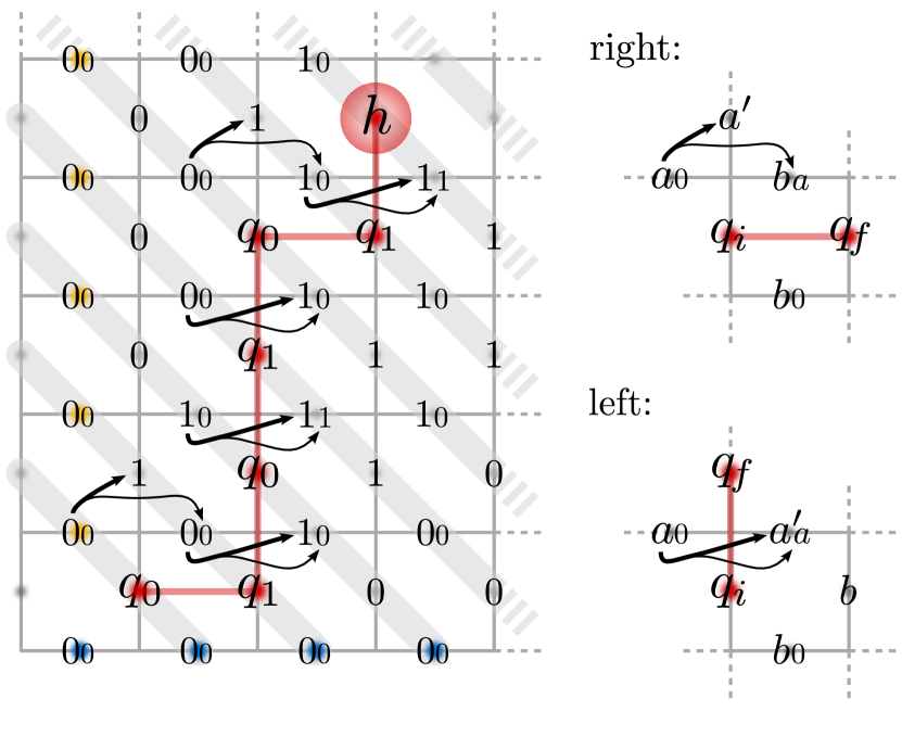
Each right transition or left transition is translated into a pair of 4-local plaquette and star interactions, as depicted to the right. Observe how in both cases the tile part of the interaction has to know the initial symbol , which is why the star operator creates a temporary copy of it. This copy is shown as small symbols and numbers to the right of the actual tape content and ignored in any following transition.
As the available space grows by one symbol in both directions at each step, there is always enough tape available for the Turing machine. The coloured terms are used to initialise this spare tape to . Away from the head, additional interactions are used to copy currently unused tape segments forward. The exact construction with all interaction terms is explained in detail in the appendix.
The maximum number of steps any halting Turing machine with states and symbols can take before halting is called the Busy Beaver number and is denoted by . Defined in [42], it is known to grow faster than any computable function. The staggering threshold sizes in table 1 show that there is no hope to address the question of extrapolating physical properties of a general system solely with an increase in computational power.
.8 Combining Hamiltonian Spectra
Lemma 3.
Let and two local Hamiltonian defined on and for some interaction graph . Let further . Then there exists a Hamiltonian on with the following properties:
-
1.
Any eigenvector of with eigenvalue is given by an eigenvector of either or , extended canonically to the larger Hilbert space , with the same eigenvalue .
-
2.
is translationally invariant if and are.
-
3.
contains nearest neighbour interactions and otherwise leaves the interaction range of and intact.
Proof.
Let and be the identity operators on and , respectively. Let . Define further
where denotes any neighbouring spin pairs. Set , where and analogously for .
The last two claims are satisfied by construction. To prove the first point, note that , and commute and thus share a common eigenbasis with spectrum . Since , any eigenstate of with eigenvalue thus has to be in the kernel , and the claim follows. ∎
I Thermal stability
I.1 Stability up to Transition Threshold Size
We will now show that for both the periodic tiling and the Busy Beaver model there exists a finite inverse temperature (depending on the local dimension due to its explicit dependence on the threshold size ), above which the thermal state of the Hamiltonian will still be very close to a classical state, i.e. to the classical ground state of .
We will recall the following observation of Hastings [18]: if is the density matrix corresponding to the ground state of (i.e. ), then we have the following bound:
| (7) |
where is the ground state energy. Moreover, since , we have that
| (8) |
where eigenvalues are counted with their multiplicity.
Let us denote by the spectral gap of , and by the number of eigenstates with energy in the range . Then, following [18], if satisfies
| (9) |
then we can bound the r.h.s. of eq. 8 by
Since in our case is a commuting Hamiltonian, grows as , which implies
| (10) |
Fix a small , and let us now choose such that
where is the critical system size of , meaning that
| (11) |
With this choice of , we have that for all system sizes and all , the thermal state is -close to the ground state of , which as we have seen is a classical product state.
On the other hand, if , from the periodic tiling construction we see that the sector of corresponding to the tiling Hamiltonian necessarily picks up an energy penalty every period of (it actually picks up even more, given that the pattern is repeated vertically with a period corresponding to the number of colours, and therefore the energy penalty of every square is at least ). This implies that every eigenstate of has a strictly positive energy density, and the spectrum of is contained in . This is not true for the Busy Beaver embedding, as it could be more favourable to terminate the computation, and then simply continue with a blank tape. The energy density decreases to zero in this case. Augmenting the construction with a base layer formed from Robinson tiles, it is however possible to make this Turing machine embedding similarly robust. We refer the reader to [45] and [12, ch. 8] for more details.
I.2 Thermodynamic Limit
Let us now recall that a state in the thermodynamic limit is given by a linear, positive and normalised functional on the algebra of quasi-local observables , which is the (norm closure of the) inductive limit of the finite matrix algebras , where is an ascending sequences of finite lattices converging to [6, 1].
Given a local Hamiltonian and a finite region , we define its (exterior) boundary as the set of sites in the complement of for which there is an interaction term in acting non-trivially on sites of and simultaneously, as shown in fig. 5. is defined as and, for a region , will denote the restriction of to all interactions which are totally contained in . A ground state is then defined as a state functional , such that for any finite , and any local observable ,
| (12) |
This definition can be obtained by taking the zero temperature limit in the definition of finite temperature equilibrium states as defined by the KMS condition (i.e. the limit of increasing-volume Gibbs ensembles satisfying the KMS condition, see [17, eq. 4.2]). Loosely speaking, it expresses the intuitive understanding that any local perturbation should not decrease the energy of a ground state (see [11]).
Note that since both and have finite support, it is possible to rewrite eq. 12 in terms of the reduced density matrix of over , which we denote by :
or equivalently
| (13) |
for all and all . In turn, this implies that
| (14) |
for any completely positive, trace preserving linear map , as can be seen by applying eq. 13 to the Kraus operators of .
We will argue that the only ground states of the periodic tiling Hamiltonian are the ground states of the Toric Code. This in turns implies, that if we take first the limit of going to infinity, and then we send the temperature to zero, we recover only ground states of the Toric Code.
Key to our argument is that part of our Hamiltonian—i.e. —is a ferromagnetic Ising-type interaction, where spin up and down are now the tiling and Toric code subspaces, respectively. We will follow the same proof technique used to show that the 2D Ising model with an external magnetic field has a unique ground state [1, ex. 5] to show that any ground state in the thermodynamic limit of our model is completely in the Toric code subspace, by which we mean that for all , for the projector onto the Toric code subspace supported on .
Let us start with some preliminary observations, which will allow us to assume some extra properties of the ground state without loss of generality. Fix and let be a decomposition of the identity on into orthogonal projectors, such that for all . We want to show that is sufficient to study restricted to the subspace corresponding to each . This is the content of the following lemma.
Lemma 4.
Let be a ground state. Fix and let be as above. Whenever , define by
Then is also a ground state. Moreover, if for every it holds that , then also .
Proof.
is clearly a positive linear functional on local observables so that . It can then be extended to a state on . The fact that commutes with the Hamiltonian makes trivially fulfil eq. 12, so it is a ground state. Finally, we observe that
so that the last claim of the lemma follows. ∎
We will use such lemma to make two extra assumptions. The first one allows to assume that the ground state is supported, in each site, only in one of the two subspaces (TC or tiling). For that, given a finite region we consider signatures where each . We denote by the projector onto the set of states of signature . It is easy to see that they satisfy the condition of lemma 4. The second assumption is that commutes with the Toric Code stabilisers. Again, it is sufficient to consider the projectors onto the eigenspaces of such stabilisers, and the result follows from lemma 4.
As a second step, we will show that for any ground state for which a square boundary is completely supported in the TC subspace, the interior will be as well; for this we will assume that all square regions have smooth edges as in fig. 5.
Lemma 5.
Take two concentric square regions , and a ground state of with a signature on . Assume that on all sites of . Moreover, assume that commutes with the Toric Code stabilisers that couple with . Then all sites .
Proof.
Denote with the set of all sites that satisfy .
Consider the CPTP map acting on that on all those sites, traces out the tiling sector and replaces it with the maximally mixed state on the TC subspace, i.e.
Let us now consider a map , acting on , which implements the following operations: first measures the Toric Code projectors which overlap with , and then, conditioned on the syndrome of the measurement, applies a unitary operator which corrects as many as code errors as possible 555One possible way to implement this procedure is to follow a sequence of local steps along an oriented tree structure, as described in [13]. This can be constructed by choosing as Kraus operators of the product of the projector onto the different syndrome subspaces multiplied on the left with the corresponding unitary operator. We extend this map on the tiling subspace with the identity map, in order to make it a CPTP map. Then eq. 14 implies that
| (15) |
We now consider . For any whose support is disjoint from , we have that since has the same reduced density matrix as outside of . Thus eq. 15 reduces to , where in only those local Hamiltonian terms appear whose support intersects with . To finish the proof, we need to find a contradiction assuming that is not empty. First of all, notice that is completely supported on the TC subspace in , and that can violate at most 2 of the Toric Code stabilisers (at most one plaquette and one star operator, since any pair of violation would have been destroyed by the action of ). So can at most be equal to 2. On the other hand, even with the bonus gained in bottom-left corners of regions supported on the tiling subspace (i.e. the bonus of for the all-black tile used to resolve the ground state degeneracy for the periodic tiling pattern), the penalties coming from mixed signatures in are higher (an overall penalty of at least for each mismatch). ∎
In the next lemma, we generalise the previous one for the case in which some sites on are in the tiling sector.
Lemma 6.
Take two concentric square regions , and a ground state of with a signature on . Moreover, assume that commutes with the Toric Code stabilisers that couple with . Let be the number of sites for which , and the sum of signature mismatches within —i.e. the number of neighbouring for which —plus the number of period markers within . Then .
Proof.
We follow the same procedure as in the proof for lemma 5, obtaining a new state on , such that
| (16) |
Again, let the set of sites with tiling signature. Let us consider now the interactions in and compare the values and . As in previous lemma, if do not overlap with , then . Since is in the TC subspace, and can violate at most 2 stabilisers, its energy can be at most (the signature in has not changed, and each spin in the tiling subspace can violate up to 4 Ising-type interactions). On the other hand, since there are at least signature mismatches for , and each of them has an energy of at least (again, this is lower than because of the bonus given to the all-black tile), we have that . Inserting these two bounds into eq. 16, we obtain the desired bound. ∎
In the following, we will show that if we pick the outer square in lemma 5 large enough, we can always find an inner concentric square—of at least a third of the outer square’s size—for which we can then apply lemma 5 or lemma 6. In the pictures of the following lemma, we have coloured with black the spins which are in the TC subspace, and in yellow the ones which are not.
Lemma 7.
Take some square of side length , where and consider a ground state of with a signature on . Subdivide into squares:
Then for all in the centre .
Proof.
We start with a few preliminary observations, and we refer the reader to fig. 5 for verification. The boundary contains precisely spins on each side, and thus spins overall. We denote this spin count with in the context of this proof. By lemma 6 (assuming that for all ), we thus know that we can have at most penalties from signature mismatches or period markers within .
The overall area of encompasses tiles, and we count spins. Every sub-square of size which is not fully in the TC subspace carries a penalty —note that this holds true regardless of the bonus terms present in the tiling, as the period penalty and TC-tiling mismatch are both larger. This means that at most a fraction of
of spins can have signature . For a subset , we denote this fraction with .
So let us assume that . Take and shrink it uniformly by at most , by which we mean we shrink the square on each side by one tile at a time, i.e. while keeping smooth boundaries as in fig. 1. This sweeps a region which covers at least of the area of , and thus in particular the number of spins . Since , it follows that . This immediately implies that there exists a square concentric with and such that , and which satisfies .
Two things may happen. If in between the centre square and there exists another square (i.e. with ) such that for any , we have , then lemma 5 immediately implies that for all in the centre , and the claim follows.
It remains to analyse the case where no such square exists. We first apply lemma 6 again, this time to : as , and , we know that there exist at most spins with . But since no exists with a boundary completely with tiling signature, there have to be at least spins within with a tiling signature (one within the boundary for each concentric square between and ). Contradiction, and the claim follows. ∎
All the above results lead trivially to
Corollary 8.
All ground states of are fully supported in the TC subspace.
II Extensive Hamiltonian Perturbation
We will prove that even under extensive Hamiltonian perturbation the ground state of our model remains in the same phase as the Toric Code. In order to achieve this, we consider local perturbations of the form
where acts on sites at a distance at most from , and for some positive and . We want to show that for the local Hamiltonians we constructed, in the thermodynamic limit and for sufficiently small , the ground states of are automorphically equivalent to the ground states of (in the sense of [2]), i.e. that the ground states can be connected by locally-generated unitary transformations.
We will show this by using a modified version of the proof presented in [8], from where we take the notation and terminology in what follows, but accounting for the following key differences:
-
1.
we have open and not periodic boundary conditions,
-
2.
our Hamiltonian is not a sum of projectors, and
-
3.
before the threshold system size, the ground state does not have topological order.
In particular, regarding 1., a solution of the stability problem for topological models besides periodic boundaries is given in [33]. For the convenience of the reader, instead of just referring to [33], we detail here the concrete solution for our particular case of interest.
Let us define, for every finite and rectangular with side larger than the threshold , and ,
i.e. we only include in the perturbation terms which are at distance (to be determined later) away from the boundary. We will show that, if is smaller than some (independent of ), then will have a spectral gap of for every , and this is sufficient to prove the equivalence of the ground states of and in the thermodynamic limit [2]. For the rest of the proof, we will fix and write instead of for simplicity.
The proof strategy of [8] can be summarised as follows: the aim is to show that, if is sufficiently small, and if has a spectral gap of at least for every , then the spectral gap at is actually larger than . This “bootstrapping” procedure then immediately implies that the gap of is never zero for every . Our Hamiltonian does not have a spectral gap of as is the case in the original proof, but since it is still a constant (independent of ) a simple rescaling will be sufficient to follow the proof strategy.
As a first step to prove the “bootstrapping” argument one uses the so called quasi-adiabatic evolution [9], which allows to write a general perturbation as a block-diagonal operator with respect to the projector on the ground state of , plus some weak boundary terms; then one uses the Topological Quantum Order of the Toric Code in order to decompose a block-diagonal perturbation into a locally block-diagonal part plus a small residual perturbation.
To simplify notation, for each site we will denote the distance of from the boundary of . Given an Hermitian operator , we will often use the decomposition , where runs over the vertices in and is supported on a ball of radius around . If for some positive and some function with values in and decaying faster than any polynomial function, we will say that is quasi-local with strength . The operator , in which every term of the decomposition acts on , will be said to be supported around .
Lemma 9.
For every , has the same spectrum as
where and each is a quasi-local operator with strength supported around .
Proof.
We will write for simplicity , where each acts around (so that each plaquette and star operator is associated to one site belonging to them). The proof will follow [8, Lemma 7], with the necessary modifications: we consider the quasi-adiabatic evolution (also known as spectral flow) associated to the Hamiltonian path , generated by the operator
where is the weight function defined in [8]. The unitary is then defined by
where denotes the -ordered exponential. It is the unique solution to the differential equation
Since it is locally generated, it satisfies Lieb-Robinson bounds [26, 19, 7, 32], meaning that for a quasi-local operator with strength supported around will be mapped by to another -strength quasi-local perturbation supported around , thus preserving locality. Moreover, we see that each is a quasi-local -strength operator supported around . We can then define
Clearly has the same spectrum as , while its ground state projector is . We will use frequently the fact that the ground state projector of satisfies . Let us define
where is the filter function defined in [8, Lemma 7]. It has the property that , and therefore . Since has exponentially decaying interactions, will map quasi-local operators of strength supported around to quasi-local operators of strength supported around [8, Lemma 2]. Moreover, it is easy to see that , so we have that
where
Each of the terms appearing in the above decomposition commutes with . For each such that , let be the closest point to in such that (and we make an arbitrary choice if it is not unique). Let be the set of points which are sent to by . We can then define for each such that :
In order to conclude, we have to show that and have strength if , while is supported around with strength if , for some fast decaying function . This will guarantee that the sum is a quasi-local operator of strength around .
In order to do so, let us observe that if a quasi-local operator such that satisfies that for each , then it is also a quasi-local operator with strength supported at any point at distance from .
The terms are supported around with by construction, and they are quasi-local with strength because of Lieb-Robinson bounds applied to and to . Let us now analyse instead the terms of .
For each , we will further decompose as follows
We will now threat the two terms independently. Let us start by observing that
Because of the quasi-locality of , if the commutator will be a quasi-local Hamiltonian of strength supported around . Applying again Lieb-Robinson bounds for , this also hold for .
If instead , we can expand in terms of the local decomposition of . Any term whose support is disjoint from the support of will not contribute to the commutator, and in particular only terms with will be present. By the previous observation, it is supported around . Applying a the unitary rotation will preserve the locality and the strength, so also will be of strength supported around .
Similarly we observe that
with
which decays faster than any polynomial. Therefore
As we did before, we now use the fact that has a quasi-local structure, so that we can analyse two different cases: if , then will be quasi-local with strength , while if there will be no terms with support smaller than , so it is supported around with strength . Again, applying the rotation will not change these properties, so we have also proven that they hold for . This concludes the proof. ∎
For the second part of the proof, we will need the following lemma instead of [8, Lemma 3].
Lemma 10.
Fix a site and let be a quasi-local operator with strength supported around , and satisfying . Then we can decompose as
where , and has strength , and decays faster than any power of .
Proof.
We decompose , and by assumption decays faster than any power of . Since we choose the side of to be larger than , the ground state of is the Toric Code with open boundary condition, which satisfies topological quantum order for operators that do not act on the boundary spins. Therefore, for each , we have that is a constant multiple of . By adding constants we can assume . We define and . By construction, we have that and that decays faster than any power of . We want to show now that we can treat in the same way as in [8, Lemma 3], obtaining a decomposition , with and of strength . The original proof requires a property, denoted TQO-2, which our model satisfies only partially: if is a square contained in , and is the square containing the first and second neighbours of in , and we denote by the projector on the ground state of the Hamiltonian restricted to (i.e. considering only the interaction terms which intersect and are contained into ), then TQO-2 implies that for every operator supported on it holds that [8, Corollary 1]
| (17) |
This is only true for our model when has side larger than , since in that case is the projector on the Toric Code ground state in , which does satisfy TQO-2. We can therefore apply eq. 17 to the operator if , so in that case we obtain the following bound
| (18) |
for some decaying faster than any polynomial, and is a ball of radius centred at . We will now show how to decompose . We can consider the following decomposition of the identity , where is such ,
Since , we have that
where
Both and are Hermitian, they annihilate , and they are supported on . We are only left to show that their norm is decaying fast in . This is trivial for , since its norm is bounded by the norm of , while each of the terms in corresponding to the different choices of and can be bounded using eq. 18. Defining concludes the proof. ∎
Finally, we want to apply [8, Lemma 5] in order to prove that a perturbation which does not intersect the boundary and such that is relatively bounded by —we can use standard perturbation theory for the terms which do intersect the boundary. Again, we run into the problem that our model does not satisfy TQO-2 for regions smaller than . But we can trivially modify the proof of such Lemma, and in particular of [8, Proposition 1], by requiring that (since by construction we only have operators with such restriction on ). In that case, given a partition of into disjoint rectangular boxes of size , we can define for every binary string an operator
We say that a box is occupied if . We then see that if is an operator acting on a square of size , which does not intersect the boundary of , and such that , then if and only if intersects a box occupied in , a box occupied in , and the only differences in the configurations and are in boxes intersecting . From here we can follow verbatim the proof of [8, Proposition 1]. We can conclude then with the following lemma.
Lemma 11.
There exists a positive function , growing slower than any polynomial in , such that if for of size we have that then the spectrum of is contained in
for every , where runs over the spectrum of , , and vanishes as goes to infinity.
Proof.
Using lemma 9 and lemma 10, we see that the spectrum of is the same as the spectrum of
where has strength and satisfies , while decays faster than any power of . Then by [8, Lemma 5] with the modification presented before, the spectrum of is contained in for some .
The rest of the perturbation is treated by bounding its norm. Since in we only included perturbations that originally act at distance at least from the boundary, and that at any given distance from the boundary of there are sites, we have that the total norm of the perturbation can be bounded by , where decays faster than any polynomial and is some positive constant. Therefore, being the tail of a discrete convolution, decays faster than any polynomial in , while grows polynomially in . We can then choose growing slower than any power and still guarantee that there exists a constant which vanishes in the limit , such that the spectrum of is contained in . ∎