Generalized virial theorem for massless electrons in graphene
and other Dirac materials

Abstract

The virial theorem for a system of interacting electrons in a crystal, which is described within the framework of the tight-binding model, is derived. We show that, in particular case of interacting massless electrons in graphene and other Dirac materials, the conventional virial theorem is violated. Starting from the tight-binding model, we derive the generalized virial theorem for Dirac electron systems, which contains an additional term associated with a momentum cutoff at the bottom of the energy band. Additionally, we derive the generalized virial theorem within the Dirac model using the minimization of the variational energy. The obtained theorem is illustrated by many-body calculations of the ground state energy of an electron gas in graphene carried out in Hartree-Fock and self-consistent random-phase approximations. Experimental verification of the theorem in the case of graphene is discussed.

I Introduction

The virial theorem (VT) provides an exact relationship between mean kinetic and potential energies of classical and quantum systems when these energies are power-law functions of coordinates and momenta of the constituent particles Marc ; Weislinger . Applications of VT include estimations of various quantities in physics of atoms, molecules, solids, plasmas, and in astrophysics. Additionally, VT and its hypervirial generalizations are used to calculate matrix elements, to improve variational calculations in quantum chemistry, as well as to check and improve equations of states and electron density functionals (see Marc ; Weislinger ; Vasilev ; Levy ; Parr and references therein).

From the fundamental point of view, VT is associated with the scale transformations of the system Marc ; Gaite or with dilatations of a ground state wave function in the quantum-mechanical case Fock ; Lowdin . When a spatially confined many-particle system (for example, electron gas in a finite-sized solid) is considered, VT acquires an additional “boundary” term proportional to the thermodynamic pressure in the system Marc , that can be interpreted as a manifestation of non-Hermiticity of the Hamiltonian Abad ; Esteve . The same term appears in VT for a uniform electron gas, that can be attributed to existence of an intrinsic length scale in the system, namely, the Bohr radius March1 ; Argyres .

There is a number of materials intensively studied in recent years where electrons at low excitation energies behave as massless particles: two-dimensional graphene CastroNeto ; Kotov , surfaces of topological insulators Hasan ; Qi , three-dimensional Dirac semimetals Wehling , and Weyl semimetals, which were discovered in very recent experiments Lv ; Xu ; Yang . When Dirac electrons are massive, their kinetic energy is not a power-law function of momentum and hence VT does not provide exact relationship between kinetic and potential energies Fock ; Rose ; March2 ; Bachall . However for massless Dirac electrons with linear dispersion such relationship can be obtained.

In this article, we derive the virial theorem for Coulomb-interacting massless electrons in Dirac materials. First, on the example of graphene, we obtain general VT for electrons in a crystal, described by a tight-binding model. Then we proceed to the approximate model of massless Dirac electrons with the momentum cutoff imposed at the bottom of the valence band. The obtained theorem should be as accurate as the Dirac approximation for electron dynamics.

It is shown that massless electrons in a Dirac material disobey conventional VT but instead they can be described by the generalized virial theorem (GVT), which contains an additional term proportional to the derivative of the ground state energy with respect to the cutoff momentum. This term can be interpreted as a manifestation of the underlying crystal lattice, characterized by a definite lattice constant, during the scale transformations. The role of a periodic potential of a crystal lattice in VT for electrons was also studied in the Kronig-Penney model Weislinger2 and in the density functional context Mirhosseini . Another approach to obtain GVT presented in the article is the restricted minimization of the variational energy with respect to dilatations of the ground state wave function.

The obtained GVT is illustrated in the case of graphene by the many-body diagrammatic calculations in Hartree-Fock and self-consistent random-phase approximations. It is shown that the relative contribution of the cutoff-induced term in GVT for graphene ranges from 5 to 20% at typical conditions. However, the obtained form of GVT is applicable to any other Dirac material with massless electrons near the Fermi energy.

The article is organized as follows. We derive GVT for graphene in the tight-binding model in Sec. II and obtain its approximation in the Dirac model in Sec. III. GVT for Dirac materials will also be obtained in Sec. IV by means of restricted minimization. We illustrate this theorem by many-body calculations of the ground state properties of the electron gas in graphene in Sec. V, considering separately the cutoff-induced term in Sec. VI, and make conclusions in Sec. VII.

II Virial theorem in the tight-binding model

The many-body Hamiltonian of $2\mathrm{p}_{z}$-electrons in graphene $H=H_{0}+H_{\mathrm{int}}+H_{\mathrm{ext}}$ includes the tight-binding nearest-neighbor kinetic energies

$$H_{0}=\sum_{i}\left(\begin{array}[]{cc}\epsilon_{0}&-tf_{\mathbf{p}_{i}}\\ -tf^{*}_{\mathbf{p}_{i}}&\epsilon_{0}\end{array}\right)_{i},$$ (3)

as well as Coulomb electron-electron interaction and interactions of electrons with the external potential $U_{\mathrm{ext}}(\mathbf{r})$:

$$H_{\mathrm{int}}=\frac{1}{2}\sum_{i\neq j}\frac{e^{2}}{\varepsilon|\mathbf{r}_{i}-\mathbf{r}_{j}|},\qquad H_{\mathrm{ext}}=\sum_{i}U_{\mathrm{ext}}(\mathbf{r}_{i}).$$ (4)

Here $\epsilon_{0}$ and $t$ are the on-site energy and the hopping integral, $f_{\mathbf{p}}=\sum_{s=1}^{3}e^{(i/\hbar)\mathbf{p}\mathbf{b}_{s}}$, where $\mathbf{b}_{s}$ are the vectors, which connect any atom from graphene sublattice $A$ with its nearest neighbors from sublattice $B$ CastroNeto ; Kotov , $\varepsilon$ is the dielectric constant of background medium; the matrix in (3) acts on sublattice degree of freedom of the $i$-th electron.

As the starting point for derivation of the virial theorem, we use, similarly to Abad ; Esteve , the following equation:

$$\langle\Psi|[H,G]|\Psi\rangle=0,$$ (5)

which is satisfied identically for any stationary state $|\Psi\rangle$ and for any operator $G$, provided the Hamiltonian $H$ is Hermitian. To obtain VT, $G$ is chosen to be the virial operator:

$$G=\sum_{i}\frac{\mathbf{r}_{i}\mathbf{p}_{i}+\mathbf{p}_{i}\mathbf{r}_{i}}{2}.$$ (6)

The commutators of each term of $H$ with $G$ can be calculated explicitly:

$$[H_{0},G]=-i\hbar\sum_{i}\mathbf{p}_{i}\frac{\partial H_{0}}{\partial\mathbf{p}_{i}},\quad[H_{\mathrm{int}},G]=-i\hbar H_{\mathrm{int}},$$ (7)

$$[H_{\mathrm{ext}},G]=i\hbar\sum_{i}\mathbf{r}_{i}\frac{\partial U_{\mathrm{ext}}(\mathbf{r}_{i})}{\partial\mathbf{r}_{i}}.$$ (8)

Now we apply the general formulas (5)–(8) to the tight-binding model, where the electron momenta $\mathbf{p}_{i}$ enter (3) only in a product with the lattice constant $a$ (since $|\mathbf{b}_{s}|=a/\sqrt{3}$), thus we can write

$$[H_{0},G]=-i\hbar a\left(\frac{\partial H_{0}}{\partial a}\right)_{\epsilon_{0},t}.$$ (9)

The derivative with respect to $a$ is taken here at $\epsilon_{0},t=\mathrm{const}$ because otherwise we would obtain unnecessary terms, which arise due to the physical dependence of $\epsilon_{0}$ and $t$ on $a$.

For the external potential $U_{\mathrm{ext}}(\mathbf{r})$, which confines electrons within a definite spatial volume, we can write: $U_{\mathrm{ext}}(\mathbf{r})=\tilde{U}(\mathbf{r}/R)$, where $R$ is the linear size of this volume. Using this relation in (8), we get:

$$[H_{\mathrm{ext}},G]=-i\hbar R\frac{\partial H_{\mathrm{ext}}}{\partial R}.$$ (10)

Substituting (7), (9), (10) to (5) and using the Hellmann-Feynman theorem, we obtain:

$$-a\left(\frac{\partial\tilde{E}}{\partial a}\right)_{\epsilon_{0},t}-\tilde{E}_{\mathrm{int}}-R\frac{\partial\tilde{E}}{\partial R}=0,$$ (11)

where $\tilde{E}=\langle\Psi|H|\Psi\rangle$ and $\tilde{E}_{\mathrm{int}}=\langle\Psi|H_{\mathrm{int}}|\Psi\rangle$ are, respectively, tight-binding ground state and interaction energies.

Eq. (11) is the tight-binding version of VT. It is derived explicitly for graphene, but can be applied for any tight-binding model with the condition that all hopping integrals and on-site energies are constant upon taking the derivative $\partial\tilde{E}/\partial a$.

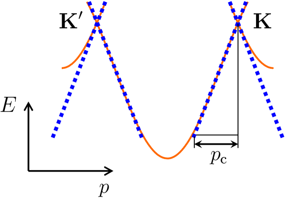
Figure 1: (Color online) Schematic tight-binding dispersion of filled single-electron states in electron-doped graphene (solid line) and its approximation in the Dirac model (dotted line). The electron states in the Dirac model are filled in both valleys $\mathbf{K}$ and $\mathbf{K}^{\prime}$ down to the cutoff momentum $p_{\mathrm{c}}$.

III Virial theorem for massless Dirac electrons

When the Fermi energy in graphene (or any other Dirac material) is close to the Dirac point, it is a reasonable approximation to switch from the tight-binding model of single-electron dynamics to the effective Dirac model CastroNeto ; Kotov ; Wehling (Fig. 1). In this model, the momentum cutoff $p_{\mathrm{c}}$ in the valence band should be introduced in order to ensure that the total density of electrons is equal to their actual density in the crystal.

The Hamiltonian of interacting massless Dirac electrons is $H=H_{\mathrm{D}}+H_{\mathrm{int}}+H_{\mathrm{ext}}$, where

$$H_{\mathrm{D}}=v_{\mathrm{F}}\sum_{ic}\left(\begin{array}[]{cc}0&cp_{x}-ip_{y}\\ cp_{x}+ip_{y}&0\end{array}\right)_{ic}$$ (14)

is the Dirac Hamiltonian of noninteracting electrons of chiralities $c=\pm 1$ and $v_{\mathrm{F}}=at\sqrt{3}/2\hbar$ is the Fermi velocity. In this approach, the total number $\tilde{N}=N_{0}+N$ of electrons that fill the energy band is a sum of the number $N_{0}\propto(R/a)^{D}$ of electrons, that fill the valence band from the cutoff momentum $p_{\mathrm{c}}$ at its bottom up to the Dirac point ($D$ is the space dimension), and the much smaller number $N$ of Dirac carriers (electrons at $N>0$ or holes at $N<0$). Similarly we can define the full energy of Dirac electrons

$$E(N)=\tilde{E}(\tilde{N})-\tilde{E}(N_{0})-\epsilon_{0}N$$ (15)

[the last term redefines the on-site energy in the Dirac single-electron Hamiltonian (14) to zero] and their interaction energy $E_{\mathrm{int}}(N)=\tilde{E}_{\mathrm{int}}(\tilde{N})-\tilde{E}_{\mathrm{int}}(N_{0})$. Note that these energies also include the energy of interaction between the $N$ Dirac electrons and the $N_{0}$ electrons of the filled valence band. Subtracting from (11) the same equation at $\tilde{N}=N_{0}$, we get:

$$-a\left(\frac{\partial{E}}{\partial a}\right)_{\tilde{N}}-E_{\mathrm{int}}-R\left(\frac{\partial E}{\partial R}\right)_{\tilde{N}}=0.$$ (16)

Hereafter we assume $\epsilon_{0},t=\mathrm{const}$ in all derivatives; we have also showed explicitly the condition $\tilde{N}=\mathrm{const}$ implied by the Hellmann-Feynman theorem for the $\tilde{N}$-particle ground state wave function.

In the Dirac model for massless electrons, the electron gas properties depend on the lattice constant $a$ indirectly via $v_{\mathrm{F}}\propto a$ and the cutoff momentum $p_{\mathrm{c}}\propto a^{-1}$ CastroNeto ; Kotov , so that the energy $E$ can be calculated as a function $E(N,v_{\mathrm{F}},p_{\mathrm{c}},R)$, where $N=\tilde{N}-N_{0}$. Consequently, the derivatives of $E$ in (16) with taking into account (15) are:

$$a\!\left(\frac{\partial{E}}{\partial a}\right)_{\!\!\tilde{N}}\!\!=-\!\left(\frac{\partial E}{\partial N}+\epsilon_{0}\right)\!a\frac{\partial N_{0}}{\partial a}+v_{\mathrm{F}}\frac{\partial E}{\partial v_{\mathrm{F}}}-p_{\mathrm{c}}\frac{\partial E}{\partial p_{\mathrm{c}}},$$ (17)

$$R\!\left(\frac{\partial{E}}{\partial R}\right)_{\!\!\tilde{N}}\!\!=-\!\left(\frac{\partial E}{\partial N}+\epsilon_{0}\right)\!R\frac{\partial N_{0}}{\partial R}+R\frac{\partial E}{\partial R}.$$ (18)

Since $N_{0}\propto(R/a)^{D}$, the first terms in right-hand sides of (17) and (18) cancel upon substituting to (16). Additionally, using the Hellmann-Feynman theorem for the kinetic energy $E_{\mathrm{kin}}=\langle\Psi|H_{\mathrm{D}}|\Psi\rangle=v_{\mathrm{F}}(\partial E/\partial v_{\mathrm{F}})$, we get the following form of GVT for massless Dirac particles:

$$-E-R\frac{\partial E}{\partial R}+p_{\mathrm{c}}\frac{\partial E}{\partial p_{\mathrm{c}}}=0,$$ (19)

where $N=\mathrm{const}$ during differentiations. The specific character of electrons with linear dispersion and Coulomb interaction is revealed in the fact that kinetic and interaction energies enter VT with the same coefficients, yielding the full energy $E=E_{\mathrm{kin}}+E_{\mathrm{int}}$ Footnote1 ; that reflects the absence of intrinsic length parameter in the system. The only length parameter is introduced by the crystal lattice via the cutoff momentum, $p_{\mathrm{c}}$, which provides the last term in GVT (19).

The second term in (19) can be related to the pressure $p=-(\partial E/\partial V)_{N}$ of the electron gas,

$$-R\frac{\partial E}{\partial R}=DpV,$$ (20)

where $V\propto R^{D}$ is the $D$-dimensional volume of the system.

In the case of a homogeneous electron gas, assuming extensiveness of the energy $E=R^{D}\epsilon(N/R^{D})$ with respect to the $D$-dimensional volume $V\propto R^{D}$, we have:

$$R\frac{\partial E}{\partial R}=DE-DN\frac{\partial E}{\partial N},$$ (21)

therefore GVT (19) takes the form:

$$-(D+1)E+DN\frac{\partial E}{\partial N}+p_{\mathrm{c}}\frac{\partial E}{\partial p_{\mathrm{c}}}=0,$$ (22)

where $R=\mathrm{const}$.

For some calculations in the limit $T\rightarrow 0$, it is more convenient to switch to the grand canonical ensemble, where the state of the system is characterized by the (zero-temperature) grand thermodynamic potential $\Omega=E-\mu N$. The Legendre transformation

$$E(N,p_{\mathrm{c}})=\Omega(\mu,p_{\mathrm{c}})+\mu N$$ (23)

implies the relations $\partial E/\partial N=\mu$, $\partial\Omega/\partial\mu=-N$, $\partial E/\partial p_{\mathrm{c}}=\partial\Omega/\partial p_{\mathrm{c}}$, that, upon substituting in (22), provide GVT in terms of $\Omega$:

$$-(D+1)\Omega+\mu\frac{\partial\Omega}{\partial\mu}+p_{\mathrm{c}}\frac{\partial\Omega}{\partial p_{\mathrm{c}}}=0.$$ (24)

Extensiveness of the thermodynamic potential allows to relate it to the pressure: $\Omega=-pV$.

The chemical potential $\mu$ in Dirac electron systems is usually measured from the Dirac point, which implies $\mu=0$ at $N=0$ (with regard to graphene it is a charge neutrality point). However, generally it is not the case for a system of interacting electrons, i.e. the “background” chemical potential

$$\mu_{0}=\left.\frac{\partial E}{\partial N}\right|_{N=0}$$ (25)

is not zero. For example, in the case of graphene,

$$\mu_{0}=-\frac{e^{2}p_{\mathrm{c}}}{2\varepsilon\hbar}$$ (26)

in the Hartree-Fock approximation Hwang .

In Appendix A, the energy $E$ and the thermodynamic potential $\Omega$ are regularized in order to remove the contributions of $\mu_{0}$. The virial theorems (48), (50), expressed in terms of these regularized quantities, are derived and shown to have the same form as (22), (24) due to the relation $\mu_{0}\propto p_{\mathrm{c}}$.

IV Restricted minimization

GVT for Dirac electrons (19) can be obtained directly by minimizing the energy with respect to dilatations of the ground state wave function, similarly to its original variational derivation in Fock ; Lowdin . Let

$$\Psi_{\lambda}(\mathbf{r}_{1}\ldots\mathbf{r}_{N})=\frac{1}{\lambda^{ND/2}}\Psi\left(\frac{\mathbf{r}_{1}}{\lambda}\ldots\frac{\mathbf{r}_{N}}{\lambda}\right)$$ (27)

be the ground state wave function $\Psi$, which is stretched by a factor of $\lambda$ uniformly in all directions. Without resorting to the coordinate representation, we can write $|\Psi_{\lambda}\rangle=D_{\lambda}|\Psi\rangle$, where

$$D_{\lambda}=\exp\left\{-\frac{i}{\hbar}G\ln\lambda\right\}$$ (28)

is the dilatation operator Abad ; Carinena and $G$ is given by (6).

Since the energies of Dirac particles are unbounded from below, we cannot minimize $\langle\Psi_{\lambda}|H|\Psi_{\lambda}\rangle$ to obtain the ground state. One of the possible ways to overcome this obstacle, which is most appropriate to the physical problem of a Dirac electron gas in a solid (Fig. 1), is to impose the momentum cutoff, requiring that all electron momenta in the many-body state $|\Psi\rangle$ do not exceed $p_{\mathrm{c}}$. This can be achieved by using the operator $P_{p_{\mathrm{c}}}$ which projects the many-body state vector on a subspace of Slater determinants, that consists of all possible single-particle plane-wave states with momenta $|\mathbf{p}|\leq p_{\mathrm{c}}$ (see Appendix B).

Although the ground state $|\Psi\rangle$ belongs to the subspace of $P_{p_{\mathrm{c}}}$, i.e. $P_{p_{\mathrm{c}}}|\Psi\rangle=|\Psi\rangle$, the dilated state $|\Psi_{\lambda}\rangle$ generally does not belong to this subspace. Therefore, in our restricted minimization procedure, we need to return $|\Psi_{\lambda}\rangle$ back into the subspace at every $\lambda$, acting on it by $P_{p_{\mathrm{c}}}$ and normalizing the resulting variational state vector. The variational energy

$$E_{\lambda}=\frac{\langle\Psi|D_{\lambda}^{-1}P_{p_{\mathrm{c}}}HP_{p_{\mathrm{c}}}D_{\lambda}|\Psi\rangle}{\langle\Psi|D_{\lambda}^{-1}P_{p_{\mathrm{c}}}D_{\lambda}|\Psi\rangle},$$ (29)

which is obtained via this restriction procedure, must have a minimum in the ground state, when $\lambda=1$, thus its derivative in $\lambda$ must vanish:

$$\left.\frac{\partial E_{\lambda}}{\partial\lambda}\right|_{\lambda=1}\!\!\!\!=-\frac{i}{\hbar}\langle\Psi|[P_{p_{\mathrm{c}}}HP_{p_{\mathrm{c}}},G]-E[P_{p_{\mathrm{c}}},G]|\Psi\rangle=0.$$ (30)

Here we used (28) and denoted $E=E_{\lambda=1}$.

The second term in (30) vanishes because $P_{p_{\mathrm{c}}}|\Psi\rangle=|\Psi\rangle$ for the ground state. The first term, with a help of (57), can be presented as

$$[P_{p_{\mathrm{c}}}HP_{p_{\mathrm{c}}},G]=P_{p_{\mathrm{c}}}[H,G]P_{p_{\mathrm{c}}}+i\hbar p_{\mathrm{c}}\frac{\partial}{\partial p_{\mathrm{c}}}(P_{p_{\mathrm{c}}}HP_{p_{\mathrm{c}}}).$$ (31)

Using the Hellmann-Feynman theorem, Eq. (30) will result in

$$\left.\frac{\partial E_{\lambda}}{\partial\lambda}\right|_{\lambda=1}\!\!\!\!=-\frac{i}{\hbar}\langle\Psi|[H,G]|\Psi\rangle+p_{\mathrm{c}}\frac{\partial E}{\partial p_{\mathrm{c}}}=0.$$ (32)

Comparing (32) with (5), we see that the restriction, which is imposed on the state vector during minimization, results in appearance of an additional term in GVT.

For Dirac electrons with the Hamiltonian $H=H_{\mathrm{D}}+H_{\mathrm{int}}+H_{\mathrm{ext}}$, similarly to (7), (10), we have

$$[H,G]=i\hbar\left(-H_{\mathrm{D}}-H_{\mathrm{int}}-R\frac{\partial H_{\mathrm{ext}}}{\partial R}\right).$$ (33)

Substituting (33) and neglecting $\langle\Psi|H_{\mathrm{ext}}|\Psi\rangle$ (see Footnote1 ), we get the same GVT for Dirac particles (19) as obtained in Sec. III from the tight-binding model.

Alternatively, instead of imposing the hard cutoff $|\mathbf{p}|<p_{\mathrm{c}}$, we can supplement the Hamiltonian with the term

$$\Delta H=(-H_{\mathrm{D}}+A)(1-P_{p_{\mathrm{c}}}),$$ (34)

which ensures that the electron states with $|\mathbf{p}|>p_{\mathrm{c}}$ have large positive energy $A$ and so pushes the ground state $|\Psi\rangle$ into the subspace of $P_{p_{\mathrm{c}}}$. In this case the system energy becomes bounded from below and the ground state $|\Psi\rangle$ becomes well-defined. Therefore we can apply the conventional VT (5) with $H+\Delta H$ instead of $H$. Using (33) and the property (57), we get:

$$\left\langle\Psi\left|-H_{\mathrm{D}}-H_{\mathrm{int}}-R\frac{\partial H_{\mathrm{ext}}}{\partial R}-Ap_{\mathrm{c}}\frac{\partial P_{p_{\mathrm{c}}}}{\partial p_{\mathrm{c}}}\right|\Psi\right\rangle$$

$$+\langle\Psi|H_{0}(1-P_{p_{\mathrm{c}}})|\Psi\rangle=0.$$ (35)

The last term is proportional to the part $(1-P_{p_{\mathrm{c}}})|\Psi\rangle$ of the ground state vector, which goes beyond the low-energy subspace of $|\Psi\rangle$ and thus behaves as $\sim 1/A$ at $A\rightarrow\infty$. Then if we apply the Hellmann-Feynman theorem to $\partial E/\partial R$ and $\partial E/\partial p_{\mathrm{c}}$, and tend to the limit $A\rightarrow\infty$, we again obtain GVT (19).

This last method does not require $P_{p_{\mathrm{c}}}|\Psi\rangle=|\Psi\rangle$ in the ground state, which is, generally, not the case in nonuniform systems where $H$ and $P_{p_{\mathrm{c}}}$ do not commute.

V Many-body calculations for graphene

In the case of graphene, we can illustrate GVT (19) with many-body calculations of the ground state energy $E$. Throughout Secs. V and VI we assume $D=2$ and use the symbol $S$ instead of $V$ for a two-dimensional volume (area).

As known, the interaction-induced correction $\delta\Omega=\Omega-\Omega_{0}$ to the grand thermodynamic potential $\Omega(\mu)$ at given chemical potential $\mu$ can be calculated as a sum of closed connected diagrams Abrikosov ; Mahan ; $\Omega_{0}(\mu)$ is the thermodynamic potential of the noninteracting electron gas. Summation of infinite diagrammatic series is usually carried out by means of Dyson equations, where bare Green functions are replaced with the dressed ones; thus the diagrammatic calculations become self-consistent. Analogous replacements in closed diagrams for $\delta\Omega$ produce excess terms, which, however, can be compensated by using the Luttinger-Ward functional Luttinger (see its application for graphene in Lozovik ).

Here we use another approach, also described in Luttinger : at $T=0$ in the spherically-symmetric system, self-consistent calculation of the ground state energy $E(N)$ at given electron number $N$ can be carried out according to the formula

$$E(N)=\Omega_{0}(\mu_{0}(N))+\mu_{0}(N)N+\delta\Omega_{\mathrm{BG}}(\mu_{0}(N)),$$ (36)

where $\mu_{0}(N)$ is the chemical potential of a noninteracting electron gas at given $N$ and $\delta\Omega_{\mathrm{BG}}(\mu)$ is the Brueckner-Goldstone sum of all closed connected diagrams except the “anomalous” ones Footnote2 calculated at given chemical potential $\mu$. This approach reduces the problem of self-consistent diagrammatic calculations of $\delta\Omega$ to a simpler problem of non-self-consistent calculations of the diagrammatic series $\delta\Omega_{\mathrm{BG}}$.

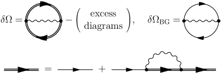
Figure 2: The diagrams presenting the interaction-induced correction $\delta\Omega$ to the thermodynamic potential and its Brueckner-Goldstone part $\delta\Omega_{\mathrm{BG}}$, which contains no “anomalous” diagrams, in the Hartree-Fock approximation. Thin and thick straight lines are bare and dressed electron Green functions, wiggly line is the Coulomb interaction.

We apply this approach to the Dirac electron gas in graphene to calculate $E$ in the Hartree-Fock and self-consistent random-phase approximations. In the Hartree-Fock approximation, the self-consistently evaluated thermodynamic potential (Fig. 2) can be calculated using (36), where the Brueckner-Goldstone perturbation series is reduced to a single first-order diagram. In the self-consistent random-phase approximation (Fig. 3), we take into account all possible diagrams without vertex corrections. The corresponding Brueckner-Goldstone perturbation series is presented by the sum of non-self-consistent random-phase approximation diagrams that can be calculated analytically Barlas .

Having analytical results for $\delta\Omega_{\mathrm{BG}}$ in both approximations (see Hwang ; Barlas and also Lozovik ), we can calculate the ground state energy (36) and substitute it into GVT (19). Following the lines of Appendix A, we omit the large constant term (26) in the chemical potential, which appears due to exchange with the filled valence band and thus actually work with the regularized energy (46) and GVT (48).

In our calculations, we use the following parameters: the bare Fermi velocity is $v_{\mathrm{F}}=0.9\times 10^{6}\,\mbox{m/s}$, as retrieved from the comparison of theory and experimental data on graphene quantum capacitance Lozovik . For the cutoff momentum, we assume the value $p_{\mathrm{c}}/\hbar=1.095\,\mbox{\AA}^{-1}$, found by equating the density of valence-band electrons $2/S_{0}$ to the same density in the Dirac model $gp_{\mathrm{c}}^{2}/4\pi\hbar^{2}$, where $S_{0}=a^{2}\sqrt{3}/2$ is the area of graphene elementary cell and $g=4$ is the degeneracy factor. For the dielectric constant $\varepsilon$ we take $\varepsilon=1$ (suspended graphene), $\varepsilon=4.5$ (encapsulation in hBN), and $\varepsilon=8$ (some medium with stronger screening).

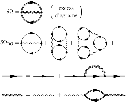
Figure 3: The same as Fig. 2, but in the self-consistent random-phase approximation. Thick wiggly line is the screened Coulomb interaction.

Our results for uniform Dirac electron gas of the density $n=N/S$ are presented in Fig. 4(a). The first term in GVT (19), i.e. the ground state energy $E$, is plotted with thick lines. In the absence of both scale-invariance breaking factors, namely, the system boundary and the momentum cutoff, we would obtain $E=0$. Thus the nonzero value of $E$ demonstrates the role of these factors. Adding the boundary term, we get the quantity $E+R(\partial E/\partial R)=p_{\mathrm{c}}(\partial E/\partial p_{\mathrm{c}})$, which would be zero in the absence of momentum cutoff, if conventional VT would have been applicable to graphene. Thus nonzero value of $p_{\mathrm{c}}(\partial E/\partial p_{\mathrm{c}})$ [shown in Fig. 4(a) with thin lines] demonstrates the degree of violation of conventional VT in graphene due to the momentum cutoff.

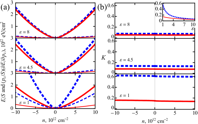
Figure 4: (Color online) (a) Ground state energy of electron gas in graphene per unit area $E/S$ (thick lines) and its derivative $(p_{\mathrm{c}}/S)(\partial E/\partial p_{\mathrm{c}})$ (thin lines), calculated as functions of carrier density $n$ at different values of $\varepsilon$. (b) The normalized derivative $K=(p_{\mathrm{c}}/E_{0})(\partial E/\partial p_{\mathrm{c}})$, as defined by (37). All curves present calculations in the Hartree-Fock (dashed lines) and self-consistent random-phase (solid line) approximations. Inset: $K$ at $n\rightarrow 0$ as a function of the dielectric constant $\varepsilon$.

As we can see, both approximations show similar results at large $\varepsilon$ and disagree at $\varepsilon\rightarrow 1$. The Hartree-Fock approximation always predicts stronger influence of the scale-invariance breaking terms. At moderate dielectric constants $\varepsilon\gtrsim 2$, the momentum cutoff provides much smaller contribution to GVT than the boundary of the system, as demonstrated in Fig. 4(a) where the thick curves pass much higher than the thin ones.

VI Cutoff-induced term in the case of graphene

Consider the ratio

$$K=\frac{p_{\mathrm{c}}}{E_{0}}\frac{\partial E}{\partial p_{\mathrm{c}}}$$ (37)

of the cutoff-induced term in GVT (19) to the energy

$$E_{0}=\frac{4}{3}\sqrt{\frac{\pi}{g}}S\hbar v_{\mathrm{F}}|n|^{3/2}$$ (38)

of the noninteracting Dirac electron gas. Explicit calculations of the ground state energy $E$ provide the following analytical forms of this ratio:

$$K=\frac{r_{\mathrm{s}}}{4}+\mathcal{O}\left(\frac{p_{\mathrm{F}}}{p_{\mathrm{c}}}\right)$$ (39)

in the Hartree-Fock approximation and

$$K=\frac{r_{\mathrm{s}}}{4}+\frac{3}{2\pi g}a(gr_{\mathrm{s}})+\mathcal{O}\left(\frac{p_{\mathrm{F}}}{p_{\mathrm{c}}}\right)$$ (40)

in the self-consistent random-phase approximation. Here $r_{\mathrm{s}}=e^{2}/\varepsilon\hbar v_{\mathrm{F}}$ is the effective fine-structure constant for graphene, $p_{\mathrm{F}}=\hbar\sqrt{4\pi|n|/g}$ is the Fermi momentum; the function $a(gr_{\mathrm{s}})$ was described in Lozovik .

The formulas (39)–(40) show that the cutoff-induced term $p_{\mathrm{c}}(\partial E/\partial p_{\mathrm{c}})$ in (19) becomes proportional to $E_{0}$ in the limit $p_{\mathrm{c}}\rightarrow\infty$ or $|n|\rightarrow 0$. In the range of carrier densities $|n|\lesssim 10^{13}\,\mbox{cm}^{-2}$, which is accessible in experiments using the electric field effect, their ratio $K$ indeed weakly depends on $n$, as shown in Fig. 4(b). The magnitude of $K$, ranging from 5 to 20% at typical values of $\varepsilon$ [see the inset in Fig. 4(b)], demonstrates the relative contribution of the scale-invariance breaking momentum cutoff to GVT in the case of graphene.

Moreover, the quantity $K$ can be related directly to observable characteristics of the electron gas. Differentiating GVT in the form (22) at $D=2$ with respect to $N$, assuming $\partial K/\partial N\approx 0$ and using (38), we get:

$$2n^{2}\frac{d\mu}{dn}-\mu n=\frac{3}{2}\frac{E_{0}}{S}K,$$ (41)

where $\partial E/\partial N=\mu$ and $K$ can be taken at $|n|\rightarrow 0$. Since $E_{0}\propto|n|^{3/2}$ according to (38), we get:

$$\lim_{|n|\rightarrow 0}\frac{2n^{2}(d\mu/dn)-\mu n}{|n|^{3/2}}=\sqrt{\frac{4\pi}{g}}\hbar v_{\mathrm{F}}K.$$ (42)

From this equation, using again (38), we can restore the cutoff-induced term:

$$p_{\mathrm{c}}\frac{\partial E}{\partial p_{\mathrm{c}}}\approx\frac{2}{3}S|n|^{3/2}\times\lim_{|n|\rightarrow 0}\frac{2n^{2}(d\mu/dn)-\mu n}{|n|^{3/2}}.$$ (43)

The quantities in the right hand side of this formula can be evaluated from experimentally observable characteristics: $d\mu/dn$ is related to compressibility and quantum capacitance (see Lozovik and references therein), while $\mu$ can be found by integrating $d\mu/dn$. Thus the cutoff-induced term in GVT (19) can be both extracted from experimental data [using (43)] and calculated theoretically [using diagrammatic approach or the approximate formulas (39)–(40)].

VII Conclusions

We have addressed the problem of quantum-mechanical many-body virial theorem for electrons in a periodic crystal lattice. First, we derive VT, which is applicable for electrons described by an arbitrary tight-binding model (11). Then we proceed to the model of massless Dirac particles with linear dispersion and a momentum cutoff imposed at the bottom of the valence band, and derive GVT (19) for this system as well as its grand canonical counterpart (24). GVT for massless Dirac electrons includes the additional term $p_{\mathrm{c}}(\partial E/\partial p_{\mathrm{c}})$, which is absent in the case of usual electron gas. The equations (11), (19), and (24) are the main results of our paper.

Alternative ways to obtain GVT, which start immediately from the Dirac model, were demonstrated. We considered the Dirac particles with the momentum cutoff $|\mathbf{p}|<p_{\mathrm{c}}$ imposed in order to bound the system energy from below. In this case GVT can be obtained by means of restricted minimization (29)–(30) of the variational energy with respect to dilatations of the ground state wave function. Another way is to add an additional term (34) to the Dirac Hamiltonian, which expels electrons from the states with momenta $|\mathbf{p}|>p_{\mathrm{c}}$. Note that GVT can also be deduced by means of diagrammatic or dimensional analysis, that will be considered elsewhere.

We analyzed GVT on the example of massless electrons in graphene, where the ground state energy was calculated by means of diagrammatic perturbation series. Using the method of Luttinger and Ward Luttinger , we calculated the ground state energy in the Hartree-Fock and self-consistent random-phase approximations. Our analysis shows that the relative contribution of the cutoff-induced term $p_{\mathrm{c}}(\partial E/\partial p_{\mathrm{c}})$, which enters GVT, is about 5–20% in the case of graphene. Note that our results for GVT for Dirac materisls are cardinally different from those in Stokes , where independence of $r_{\mathrm{s}}$ in graphene on electron density was not properly taken into account.

The obtained GVT demonstrates the role of two physical factors, which break the scale invariance of the system: its finite boundary and momentum cutoff. These factors restrict electron motion in coordinate and momentum spaces and manifest themselves through corresponding terms in GVT. In the case of graphene, GVT can be verified experimentally as described in Sec. VI. Possible applications of the obtained theorem can include checking the validity of “relativistic” density functional calculations of ground state properties of disordered graphene Rossi ; Polini ; Rodriguez-Vega . In addition, the tight-binding version of VT or its hypervirial generalizations can be applied to study the properties of interacting electrons in other crystals.

Appendix A Chemical potential at Dirac point $\mu_{0}$

First, let us take the derivative of (22) with respect to $N$ at $N=0$:

$$\left.\left(-\frac{\partial E}{\partial N}+p_{\mathrm{c}}\frac{\partial^{2}E}{\partial N\partial p_{\mathrm{c}}}\right)\right|_{N=0}=0.$$ (44)

Changing the order of derivatives and using (25), we get

$$p_{\mathrm{c}}\frac{\partial\mu_{0}}{\partial p_{\mathrm{c}}}=\mu_{0}$$ (45)

and thus $\mu_{0}\propto p_{\mathrm{c}}$.

Then we can regularize the energy of the Dirac electron gas in the following way:

$$E_{\mathrm{reg}}=E-\mu_{0}N.$$ (46)

According to (25),

$$\left.\frac{\partial E_{\mathrm{reg}}}{\partial N}\right|_{N=0}=0.$$ (47)

Substituting (46) to (22), we get GVT in terms of the regularized energy:

$$-(D+1)E_{\mathrm{reg}}+DN\frac{\partial E_{\mathrm{reg}}}{\partial N}+p_{\mathrm{c}}\frac{\partial E_{\mathrm{reg}}}{\partial p_{\mathrm{c}}}=0,$$ (48)

which has the same form as (22) due to the relation (45).

Finally, using the Legendre transformation

$$E_{\mathrm{reg}}(N,p_{\mathrm{c}})=\Omega_{\mathrm{reg}}(\mu_{\mathrm{reg}},p_{\mathrm{c}})+\mu_{\mathrm{reg}}N$$ (49)

we can convert (48) to GVT in terms of the regularized thermodynamic potential:

$$-(D+1)\Omega_{\mathrm{reg}}+\mu_{\mathrm{reg}}\frac{\partial\Omega_{\mathrm{reg}}}{\partial\mu_{\mathrm{reg}}}+p_{\mathrm{c}}\frac{\partial\Omega_{\mathrm{reg}}}{\partial p_{\mathrm{c}}}=0,$$ (50)

where

$$\mu_{\mathrm{reg}}=\frac{\partial E_{\mathrm{reg}}}{\partial N}$$ (51)

is the regularized chemical potential. According to (47), $\mu_{\mathrm{reg}}=0$ at $N=0$, as it should be when the chemical potential is measured from the Dirac point.

Appendix B Operator of momentum cutoff $P_{p_{\mathrm{c}}}$

Action of $P_{p_{\mathrm{c}}}$ on a many-body wave function can be represented as:

$$P_{p_{\mathrm{c}}}\Psi(\mathbf{r}_{1}\ldots\mathbf{r}_{N})=\int d\mathbf{r}_{1}^{\prime}\ldots\mathbf{r}_{N}^{\prime}K_{p_{\mathrm{c}}}(\mathbf{r}_{1}-\mathbf{r}_{1}^{\prime})$$ (52)

$$\times K_{p_{\mathrm{c}}}(\mathbf{r}_{2}-\mathbf{r}_{2}^{\prime})\ldots K_{p_{\mathrm{c}}}(\mathbf{r}_{N}-\mathbf{r}_{N}^{\prime})\Psi(\mathbf{r}_{1}^{\prime}\ldots\mathbf{r}_{N}^{\prime}).$$ (53)

An integral operator with the kernel

$$K_{p_{\mathrm{c}}}(\mathbf{r})=\int\limits_{|\mathbf{p}|<p_{\mathrm{c}}}\frac{d\mathbf{p}}{(2\pi\hbar)^{D}}\,e^{\frac{i}{\hbar}\mathbf{pr}}$$ (54)

projects a one-particle wave function onto a subspace of momenta $|\mathbf{p}|<p_{\mathrm{c}}$; this kernel has the scale property:

$$K_{p_{\mathrm{c}}}(\lambda\mathbf{r})=\frac{1}{\lambda^{D}}K_{\lambda p_{\mathrm{c}}}(\mathbf{r}).$$ (55)

Using it in (53), we get the following scale property of $P_{p_{\mathrm{c}}}$:

$$D_{\lambda}^{-1}P_{p_{\mathrm{c}}}D_{\lambda}=P_{\lambda p_{\mathrm{c}}}.$$ (56)

For infinitesimal dilatations ($\lambda\rightarrow 1$) we get, according to (28), that:

$$[P_{p_{\mathrm{c}}},G]=i\hbar p_{\mathrm{c}}\frac{\partial P_{p_{\mathrm{c}}}}{\partial p_{\mathrm{c}}}.$$ (57)

References

- (1) G. Marc and W.G. McMillan, The virial theorem, Adv. Chem. Phys. 58, 209 (1985).
- (2) E. Weislinger and G. Olivier, The classical and quantum mechanical virial theorem, Int. J. Quantum Chem. 8(S8), 389 (1974).
- (3) B.V. Vasil ev and V.L. Lyuboshits, Virial theorem and some properties of the electron gas in metals, Phys.-Usp. 37, 345 (1994).
- (4) M. Levy and J.P. Perdew, Hellmann-Feynman, virial, and scaling requisites for the exact universal density functionals. Shape of the correlation potential and diamagnetic susceptibility for atoms, Phys. Rev. A 32, 2010 (1985).
- (5) R.G. Parr and Y. Weitao, Density-functional theory of atoms and molecules (Oxford Univ. Press, New York, 1989).
- (6) J. Gaite, The relativistic virial theorem and scale invariance, Phys.-Usp. 56, 919 (2013).
- (7) V. Fock, Bemerkung zum Virialsatz, Z. Phys. 63, 855 (1930).
- (8) P.-O. Löwdin, Scaling problem, virial theorem, and connected relations in quantum mechanics, J. Mol. Spectrosc. 3, 46 (1959).
- (9) J. Abad and J.G. Esteve, Generalized virial theorem for compact problems, Phys. Rev. A 44, 4728 (1991).
- (10) J.G. Esteve, F. Falceto, and P.R. Giri, Boundary contributions to the hypervirial theorem, Phys. Rev. A 85, 022104 (2012).
- (11) N.H. March, Kinetic and potential energies of an electron gas, Phys. Rev. 110, 604 (1958).
- (12) P.N. Argyres, Virial theorem for the homogeneous electron gas, Phys. Rev. 154, 410 (1967).
- (13) A.H. Castro Neto, F. Guinea, N.M.R. Peres, K.S. Novoselov, and A.K. Geim, The electronic properties of graphene, Rev. Mod. Phys. 81, 109 (2009).
- (14) V.N. Kotov, B. Uchoa, V.M. Pereira, F. Guinea, and A.H. Castro Neto, Electron-electron interactions in graphene: Current status and perspectives, Rev. Mod. Phys. 84, 1067 (2012).
- (15) M.Z. Hasan and C.L. Kane, Colloquium: Topological insulators, Rev. Mod. Phys. 82, 3045 (2010).
- (16) X.L. Qu and S.-C. Zhang, Topological insulators and superconductors, Rev. Mod. Phys. 83, 1057 (2011).
- (17) T.O. Wehling, A.M. Black-Schaffer, and A.V. Balatsky, Dirac materials, Adv. Phys. 63, 1 (2014).
- (18) B.Q. Lv, H.M. Weng, B.B. Fu, X.P. Wang, H. Miao, J. Ma, P. Richard, X.C. Huang, L.X. Zhao, G.F. Chen et al., Experimental discovery of Weyl semimetal TaAs, Phys. Rev. X 5, 031013 (2015).
- (19) S.-Y. Xu, I. Belopolski, N. Alidoust, M. Neupane, G. Bian, C. Zhang, R. Sankar, G. Chang, Z. Yuan, C.-C. Lee et al., Discovery of a Weyl fermion semimetal and topological Fermi arcs, Science 7, 613 (2015).
- (20) L.X. Yang, Z.K. Liu, Y. Sun, H. Peng, H.F. Yang, T. Zhang, B. Zhou, Y. Zhang, Y.F. Guo, M. Rahn et al., Weyl semimetal phase in the non-centrosymmetric compound TaAs, Nature Phys. 11, 728 (2015).
- (21) M.E. Rose and T.A. Welton, The virial theorem for a Dirac particle, Phys. Rev. 86, 432 (1952).
- (22) N.H. March, The virial theorem for Dirac’s equation, Phys. Rev. 92, 481 (1953).
- (23) J.N. Bachall, Virial theorem for many-electron Dirac systems, Phys. Rev. 124, 923 (1961).
- (24) E. Weislinger and G. Olivier, Applications of a quantum virial theorem to Kronig and Penney’s model and to a diatomic molecule in static approximation, Int. J. Quan. Chem. 10, 225 (1976).
- (25) H. Mirhosseini, A. Cangi, T. Baldsiefen, A. Sanna, C.R. Proetto, and E.K.U. Gross, Virial theorem and exact properties of density functionals for periodic systems, Phys. Rev. B 89, 220102(R) (2014).
- (26) We omit the energy of electron interaction with the external potential because it vanishes in the bulk limit or when is approximated by potential walls, which height tends to infinity.
- (27) E.H. Hwang, B.Y.-K. Hu, and S. Das Sarma, Density dependent exchange contribution to and compressibility in graphene, Phys. Rev. Lett. 99, 226801 (2007).
- (28) J.F. Cariñena, F. Falceto, and M.F. Rañada, A geometric approach to a generalized virial theorem, J. Phys. A 45, 395210 (2012).
- (29) A.A. Abrikosov, L.P. Gor kov, and I.E. Dzyaloshinskii, Quantum field theoretical methods in statistical physics (Pergamon Press, Oxford, 1965), p. 128.
- (30) G.D. Mahan, Many-particle physics (Plenum Press, New York, 1990), p. 179.
- (31) J.M. Luttinger and J.C. Ward, Ground-state energy of a many-fermion system. II, Phys. Rev. 118, 1417 (1960).
- (32) Yu.E. Lozovik, A.A. Sokolik, and A.D. Zabolotskiy, Quantum capacitance and compressibility of graphene: The role of Coulomb interactions, Phys. Rev. B 91, 075416 (2015).
- (33) The “anomalous” diagrams, also called “rainbow” ones, contain at least two bare electron Green functions with the same momentum and frequency. When evaluated at , these diagrams seemingly vanish, but actually they provide delta-functional contributions at the Fermi surface Luttinger ; Kohn .
- (34) W. Kohn and J.M. Luttinger, Ground-state energy of a many-fermion system, Phys. Rev. 118, 41 (1960).
- (35) Y. Barlas, T. Pereg-Barnea, M. Polini, R. Asgari, and A.H. MacDonald, Chirality and correlations in graphene, Phys. Rev. Lett. 98, 236601 (2007).
- (36) J.D. Stokes, H.P. Dahal, A.V. Balatsky, and K.S. Bedell, The virial theorem in graphene and other Dirac materials, Phil. Mag. Lett. 93, 672 (2013).
- (37) E. Rossi and S. Das Sarma, Ground state of graphene in the presence of random charged impurities, Phys. Rev. Lett. 101, 166803 (2008).
- (38) M. Polini, A. Tomadin, R. Asgari, and A.H. MacDonald, Density functional theory of graphene sheets, Phys. Rev. B 78, 115426 (2008).
- (39) M. Rodriguez-Vega, J. Fischer, S. Das Sarma, and E. Rossi, Ground state of graphene heterostructures in the presence of random charged impurities, Phys. Rev. B 90, 035406 (2014).