Starobinsky-Type Inflation With Products
of Kähler Manifolds

C. Pallis & N. Toumbas Department of Physics, University of Cyprus,
P.O. Box 20537, CY-1678 Nicosia, CYPRUS
e-mail addresses:
cpallis, nick@ucy.ac.cy
Abstract

Abstract

We present a novel realization of Starobinsky-type inflation within Supergravity using two chiral superfields. The proposed superpotential is inspired by induced-gravity models. The Kähler potential contains two logarithmic terms, one for the inflaton $T$ and one for the matter-like field $S$, parameterizing the $SU(1,1)/U(1)\times SU(2)/U(1)$ Kähler manifold. The two factors have constant curvatures $-m/n$ and $2/n_{2}$, where $n$, $m$ are the exponents of $T$ in the superpotential and Kähler potential respectively, and $0<n_{2}\leq 6$. The inflationary observables depend on the ratio $2n/m$ only. Essentially they coincide with the observables of the original Starobinsky model. Moreover, the inflaton mass is predicted to be $3\cdot 10^{13}~{}{\mbox{\rm GeV}}$.

Keywords: Cosmology of Theories Beyond the Standard Model, Supergravity Models;
PACS codes: 98.80.Cq, 11.30.Qc, 12.60.Jv, 04.65.+e
\publishedinJ. Cosmol. Astropart. Phys. 05, no. 05, 015 (2016)


1 Introduction

The clarifications regarding the impact that the dust foreground has on the observations of the B-type polarization of the CMBR, offered by the recent joint analysis of the Bicep2/Keck Array and Planck data [2, 1], revitalizes the interest in the Starobinsky model [3] of inflation. This model predicts a (scalar) spectral index $n_{\rm s}\simeq 0.965$, which is in excellent agreement with observations, and a tensor-to-scalar ratio $r\simeq 0.0035$, which is significantly lower than the current upper bound. Indeed, the fitting of the data with the $\Lambda$CDM$+r$ model restricts [1] $n_{\rm s}$ and $r$ in the following ranges

$$n_{\rm s}=0.968\pm 0.0045\>\>\>\mbox{and}\>\>\>r\lesssim 0.12$$ (1.1)

at $95\%$ confidence level (c.l.), with negligible $n_{\rm s}$ running: $|a_{\rm s}|\ll 0.01$.

On the other hand, Supergravity (SUGRA) extensions of the Starobinsky-type inflation (STI), admit a plethora of incarnations [4, 6, 5, 7, 8, 9, 10, 11]. In most of them two chiral superfields, $T$ and $S$ are employed following the general strategy introduced in \crefreferee for the models of chaotic inflation. One prominent idea [5, 7] is, though, to parameterize with $S$ and $T$ the $SU(2,1)/(SU(2)\times U(1))$ Kähler manifold with constant curvature $-2/3$, as inspired by the no-scale models [13, 14]. In this context, a variety of models have been proposed in which the inflaton can be identified with either the matter-like field $S$ [5, 7, 6] or the modulus-like field $T$ [8, 7, 9, 10, 11]. We shall focus on the latter case since this implementation requires a simpler superpotential, and when connected with a MSSM version, ensures a low enough re-heating temperature, potentially consistent with the gravitino constraint [10, 16, 15].

A key issue in such SUGRA realizations of Starobinsky inflation is the stabilization of the field $S$ accompanying the inflaton. Indeed, when the symmetry of the aforementioned Kähler manifold is respected, the inflationary path turns out to be unstable against the fluctuations of $S$. The instabilities can be lifted if we add to the Kähler potential $K$ a sufficiently large quartic term $k_{S}|S|^{4}$, where $k_{S}>0$ and $|k_{S}|\sim 1$, as suggested in \creflee for models of non-minimal (chaotic) inflation [18] and applied extensively to this kind of models. This solution, however, deforms slightly the Kähler manifold [19] and is complicated to implement when more than two fields are present. In principle, all allowed quartic terms have to be considered, rendering the fluctuation analysis tedious – see e.g. \creftalk. Alternatively, we may utilize a nilpotent superfield $S$ [21], or a matter field $S$ charged under a gauged R-symmetry[19].

We propose a new solution to the stability problem that is compatible with a highly symmetric Kähler manifold. The Kähler potential involves a logarithmic function of the inflaton field $T$ with an overall negative prefactor, as required for establishing an asymptotic inflationary plateau [7, 8, 9, 10]. If the $|S|^{2}$ term is to appear in the argument of this logarithmic function, its coefficient must be negative in order to avoid negative kinetic terms. However such a negative coefficient leads to tachyonic instabilities. Therefore, we propose to split $K$ into a sum of two logarithmic functions, one involving the inflaton field $T$ and the other involving the field $S$, with negative and positive prefactors $(-{\rm NewA})$ and $n_{2}$, respectively. The term $|S|^{2}$ can now appear in the argument of the second logarithm with a positive coefficient. The prefactors $(-{\rm NewA})$ and $n_{2}$ are selected in order to establish STI, with the field $S$ acquiring a large enough, positive mass squared along the inflationary trajectory. The resulting Kähler potential gives rise to the product space $SU(1,1)/U(1)\times SU(2)/U(1)$.

We would like to comment on the possibility of realizing this type of Kähler metrics in the context of string theory. The non-compact coset factor, $SU(1,1)/U(1)$, appears in several string induced no-scale models [13, 19]. There are various classes of string inflationary models, namely D-brane inflation in warped (and unwarped) superstring compactifications, fluxbrane inflation, axion inflation, racetrack models, fibre inflation and others – see \crefliam for a thorough review and references therein. In models with a D-brane, there are moduli describing its position in the compactification manifold. Naively one would think that the full moduli space is a product space. The first factor, which is spanned by the brane position moduli, would be isomorphic to the internal compact manifold, and the second factor is a non-compact space spanned by the closed string moduli (such as the modulus controlling the size of the internal space). One could seek models in which the role of the inflaton is played by a closed string modulus, or as in \crefKKLMLT a brane position modulus. However, the stabilization of several closed string moduli requires the presence of non-trivial fluxes. And typically mixing arises between the brane position moduli with the closed string Kähler moduli – see \crefKKLMLT,liam for discussions. As a result, the closed string moduli space is fibered non-trivially over the space spanned by the brane position moduli, as exemplified by the DeWolfe-Giddings Kähler potential [24, 23]. If the internal, compactification manifold contains a spherical $SU(2)/U(1)$ factor, this must be supported by suitable 2-form flux, which might affect the brane worldvolume theory. Given this discussion, it may be difficult to realize a situation in which the field configuration manifold is globally isomorphic to the symmetric product space $SU(1,1)/U(1)\times SU(2)/U(1)$ in the context of string inflationary models. But at least locally in certain regions, the moduli space could be approximated by a product space of such form. This would require to turn on suitable fluxes in order to stabilize some of the moduli in these regions. As argued in \crefKKLMLT,liam, such a stabilization mechanism is likely to steepen the inflaton potential, halting inflation. It is thus challenging (and also interesting) to explicitly realize such a model in the context of string theory.

We implement our proposal within the framework [25, 26, 27, 28] of induced-gravity (IG) models, which are generalized to highlight the robustness of our approach. The key-ingredient of our construction is the presence of the two different exponents $n$ and $m$ of $T$ in the superpotential and the Kähler potential. We show that imposing a simple asymptotic condition on $n,m$ and ${\rm NewA}$, a Starobinsky-type inflationary potential gets generated, exhibiting an attractor behavior that depends only on the coefficient ${\rm NewA}$, which determines the curvature of the $SU(1,1)/U(1)$ Kähler manifold. Moreover, this model of inflation preserves a number of attractive features: (i) The superpotential and the Kähler potential may be fixed in the presence of an $R$-symmetry and a discrete symmetry; (ii) the initial value of the (non-canonically normalized) inflaton field can be subplanckian; (iii) the radiative corrections remain under control; and (iv) the perturbative unitarity is respected up to the reduced Planck scale [26, 29, 10, 28].

The paper is organized as follows: In Sec. 2 we generalize the formulation of STI within SUGRA IG models. In Sec. 3 we investigate totally symmetric Kähler potentials in order to find a viable inflationary scenario, which is confronted with observations in Sec. 4. Our conclusions are summarized in Sec. 5. Some mathematical notions related to the geometric structure of the Kähler manifolds encountered in our set-up are exhibited in Appendix A. Finally, Appendix B provides an analysis of the ultraviolet behavior of our models. Throughout, charge conjugation is denoted by a star (), the symbol $,z$ as subscript denotes derivation with respect to (w.r.t) $z$ and we use units where the reduced Planck scale $m_{\rm P}=2.43\cdot 10^{18}~{}{\mbox{\rm GeV}}$ is equal to unity.

2 Generalizing the Induced-Gravity Set-up in SUGRA

The realization of STI within IG models [7, 8, 10, 28, 27] requires the presence of two gauge singlet chiral superfields, the inflaton $T$ and a “stabilizer” superfield $S$, which we collectively denote by $z^{\alpha}$ ($z^{1}=T$ and $z^{2}=S$). The relevant part of the Einstein frame (EF) SUGRA action is given by [18]

$${\sf S}=\int d^{4}x\sqrt{-\widehat{\mathfrak{g}}}\left(-\frac{1}{2}\widehat{\mathcal{R}}+K_{{\alpha}{\bar{\beta}}}\widehat{g}^{\mu\nu}\partial_{\mu}z^{\alpha}\partial_{\nu}z^{*{\bar{\beta}}}-\widehat{V}\right)\,$$ (2.1a)
where the scalar field components of the superfields $z^{\alpha}$’s are denoted by the same superfield symbol, $K_{{\alpha}{\bar{\beta}}}=K_{,z^{\alpha}z^{*{\bar{\beta}}}}$ is the Kähler metric and $K^{{\alpha}{\bar{\beta}}}$ its inverse ($K^{{\alpha}{\bar{\beta}}}K_{{\bar{\beta}}\gamma}=\delta^{\alpha}_{\gamma}$). $\widehat{V}$ is the Einstein frame F–term SUGRA potential, given in terms of the Kähler potential and the superpotential $W$ by the following expression
$$\widehat{V}=e^{K}\left(K^{{\alpha}{\bar{\beta}}}D_{\alpha}WD^{*}_{\bar{\beta}}W^{*}-3{|W|^{2}}\right),$$ (2.1b)

where $D_{\alpha}W=W_{,z^{\alpha}}+K_{,z^{\alpha}}W$. Next we perform a conformal transformation [18, 32] and define the Jordan frame (JF) metric $g_{\mu\nu}$ via the relation

$$\widehat{g}_{\mu\nu}=-\left({\Omega}/{N}\right)g_{\mu\nu},$$ (2.2a)
where $\Omega$ is a frame function. In the JF, the action takes the form
$${\sf S}=\int d^{4}x\sqrt{-\mathfrak{g}}\left(\frac{\Omega}{2N}\mathcal{R}+\frac{3}{4N\Omega}\partial_{\mu}\Omega\partial^{\mu}\Omega-\frac{1}{N}\Omega K_{{\alpha}{{\bar{\beta}}}}\partial_{\mu}z^{\alpha}\partial^{\mu}z^{*{\bar{\beta}}}-V\right)\>\>\>\mbox{with}\>\>\>V=\frac{\Omega^{2}}{N^{2}}\widehat{V}\,.$$ (2.2b)

Here $\mathfrak{g}$ stands for the determinant of $g_{\mu\nu}$; $\mathcal{R}$ is the Ricci scalar curvature in JF, and $N$ is a dimensionless positive parameter that quantifies the deviation from the standard set-up [18]. Let the frame function $\Omega$ and $K$ be related by the equation

$$-\Omega/N=e^{-K/N}\>\Rightarrow\>K=-N\ln\left(-\Omega/N\right).$$ (2.3a)
Then using the on-shell expression [18] for the purely bosonic part of the auxiliary field
$${\cal A}_{\mu}=i\left(K_{\alpha}\partial_{\mu}z^{\alpha}-K_{\bar{\alpha}}\partial_{\mu}z^{*{\bar{\alpha}}}\right)/6,$$ (2.3b)
we arrive at the action
$${\sf S}=\int d^{4}x\sqrt{-\mathfrak{g}}\left(\frac{\Omega}{2N}\mathcal{R}+\left(\Omega_{{\alpha}{{\bar{\beta}}}}+\frac{3-N}{N}\frac{\Omega_{{\alpha}}\Omega_{{\bar{\beta}}}}{\Omega}\right)\partial_{\mu}z^{\alpha}\partial^{\mu}z^{*{\bar{\beta}}}-\frac{27}{N^{3}}\Omega{\cal A}_{\mu}{\cal A}^{\mu}-V\right).$$ (2.3c)
In terms of $\Omega$, the auxiliary field ${\cal A}_{\mu}$ is given by
$${\cal A}_{\mu}=-iN\left(\Omega_{\alpha}\partial_{\mu}z^{\alpha}-\Omega_{\bar{\alpha}}\partial_{\mu}z^{*{\bar{\alpha}}}\right)/6\Omega\,$$ (2.3d)

where $\Omega_{\alpha}=\Omega_{,z^{\alpha}}$ and $\Omega_{\bar{\alpha}}=\Omega_{,z^{*{\bar{\alpha}}}}$. This last form for the JF action exemplifies the non-minimal coupling to gravity, as $-\Omega/{N}$ multiplies the Ricci scalar $\mathcal{R}$. Conventional Einstein gravity is recovered at the vacuum when

$$-\langle{\Omega}\rangle/N\simeq 1.$$ (2.4)

Starting with the JF action in \ErefSfinal, we seek to realize STI, postulating the invariance of $\Omega$ under the action of a global $\mathbb{Z}_{m}$ discrete symmetry. When $S$ is stabilized at the origin, we write

$$-\Omega/N=\Omega_{\rm H}(T)+\Omega^{*}_{\rm H}(T^{*})\>\>\>\mbox{with}\>\>\>\Omega_{\rm H}(T)=c_{T}{T^{m}}+\sum_{k=2}^{\infty}\lambda_{k}{T^{km}},$$ (2.5)

where $k$ is a positive integer. If the values of $T$ during inflation are subplanckian and assuming relatively low $\lambda_{k}$’s, the contributions of the higher powers of $T$ in the expression above are very small, and so these can be dropped. As we will verify later, this can be achieved when the coefficient $c_{T}$ is large enough. Equivalently, we may rescale the inflaton setting $T\rightarrow\tilde{T}={c_{T}}^{1/m}T$. Then the coefficients $\lambda_{k}$ of the higher powers in the expression of $\Omega$ get suppressed by factors of $c_{T}^{-k}$. Thus $\mathbb{Z}_{m}$ and the requirement that the inflaton $T$ is subplanckian determine the form of $\Omega$, avoiding a severe tuning of the coefficients $\lambda_{k}$. Confining ourselves to such situations (and stabilizing $S$ at the origin), \ErefOmg1 implies that the Kähler potentials take the form

$$K_{0}=-N\ln\Big{(}f(T)+f^{*}(T^{*})\Big{)}\>\>\>\mbox{with}\>\>\>f(T)\simeq c_{T}T^{m}\,.$$ (2.6)

Eqs. (2.3a) and (2.4) require that $T$ and $S$ acquire the following vacuum expectation values

$$\langle{T}\rangle\simeq 1/(2c_{T})^{1/m},\>\>\>\mbox{and}\>\>\>\langle{S}\rangle=0\,.$$ (2.7)

These values can be obtained, if we choose the following superpotential [28, 27]:

$$W=\lambda S\left(T^{n}-1/(2c_{T})^{n/m}\right)\,,$$ (2.8)

since the corresponding F-term SUSY potential, $V_{\rm SUSY}$, is found to be

$$V_{\rm SUSY}=\lambda^{2}\left|T^{n}-1/(2c_{T})^{n/m}\right|^{2}+\lambda^{2}n^{2}\left|ST^{n-1}\right|^{2}$$ (2.9)

and is minimized by the field configuration in \Erefig1. Similarly to Refs. [10, 28], we argue that when the exponent $n$ takes integer values with $n>1$, the form of $W$ is constrained if we limit $T$ to subplanckian values, and if it respects two symmetries: (i) an $R$ symmetry under which $S$ and $T$ have charges $1$ and 00; (ii) a discrete symmetry $\mathbb{Z}_{n}$ under which only $T$ is charged. For $n=m$, $\mathbb{Z}_{m}$ becomes a symmetry of the theory and our scheme is essentially identical to those analyzed in Refs. [27, 28]. Generalizing these settings by allowing $n\neq m$, we find inflationary solutions for a variety of combinations of the parameters $n,m$ and $N$ – see \Srefres2 – including the choice $N=3$ which appears in the no-scale SUGRA models [13, 14, 5, 7]. Note, finally, that the selected $\Omega$ in \ErefOmdef does not contribute in the term involving $\Omega_{TT^{*}}$ in \ErefSfinal. We expect that our finding are essentially unaltered even if we include in the right-hand side of \ErefOmdef a term $-(T-T^{*})^{2}/2N$ [27] or $-|T|^{2}/N$ [28] which yields $\Omega_{TT^{*}}=1\ll c_{T}$. In those cases, however, the symmetry of the Kähler manifolds, studied in \Sreffhi1, regarding the $T$ sector of the models is violated.

The inflationary trajectory is determined by the constraints

$$S=T-T^{*}=0,\>\>\>\mbox{or}\>\>\>s=\bar{s}={\theta}=0,$$ (2.10)

with the last equation arising when we parameterize $T$ and $S$ as follows

$$T=\>{\phi\,e^{i{\theta}}}/{\sqrt{2}},\>\>\>\>\>\>S=\>(s+i\bar{s})/\sqrt{2}\,.$$ (2.11)

Using the superpotential in \ErefWn, we find via \ErefVsugra that, along the inflationary path, $\widehat{V}$ takes the following form:

$$\widehat{V}_{\rm I}=\widehat{V}({\theta}=s=\bar{s}=0)=e^{K}K^{SS^{*}}\,|W_{,S}|^{2}\,.$$ (2.12)

To identify the canonically normalized scalar fields, we cast their kinetic terms in \ErefSaction1 into the following diagonal form

$$K_{{\alpha}{\bar{\beta}}}\dot{z}^{\alpha}\dot{z}^{*{\bar{\beta}}}=\frac{1}{2}\left(\dot{\widehat{\phi}}^{2}+\dot{\widehat{\theta}}^{2}\right)+\frac{1}{2}\left(\dot{\widehat{s}}^{2}+\dot{\widehat{\overline{s}}}^{2}\right),$$ (2.13a)
where the dot denotes derivation w.r.t the cosmic time and the hatted fields are given by
$${d\widehat{}\phi/d\phi}=\sqrt{K_{TT^{*}}}=J,\>\>\>\widehat{{\theta}}=J\,{{\theta}}/{\phi},\>\>\>(\widehat{s},\widehat{\bar{s}})=\sqrt{K_{SS^{*}}}{(s,\bar{s})}.$$ (2.13b)

Note that the spinor components $\psi_{T}$ and $\psi_{S}$ of the $S$ and $T$ superfields must be normalized in a similar manner, i.e., $\widehat{\psi}_{S}=\sqrt{K_{SS^{*}}}\psi_{S}$ and $\widehat{\psi}_{T}=\sqrt{K_{TT^{*}}}\psi_{T}$.

It is obvious from the considerations above, that the stabilization of $S$ during and after inflation is of crucial importance for the realization of our scenario. This issue is addressed in the next section, where we specify the dependence of the Kähler potential on $S$.

3 Starobinsky-Type Inflation & Kähler Manifolds

We focus on Kähler potentials parameterizing totally symmetric manifolds consistent with the $R$ symmetry acting on $S$. In Sec. 3.1 we review the models based on the $SU(2,1)/(SU(2)\times U(1))$ coset space. Then we analyze Kähler potentials parameterizing specific product spaces: the $SU(1,1)/U(1)\times U(1)$ space in \Sref111 and the $SU(1,1)/U(1)\times SU(2)/U(1)$ space in \Sref112. Among these cases, only the last one yields a satisfactory scenario.

3.1 $SU(2,1)/(SU(2)\times U(1))$ Kähler  Manifold

A typical Kähler potential employed for implementing STI in SUGRA is

$$K_{1}=-n_{21}\ln\left(f(T)+f^{*}(T^{*})-{|S|^{2}\over n_{21}}\right),$$ (3.1)

with $n_{21}>0$. The Kähler metric $K_{{\alpha}{\bar{\beta}}}$ takes the form

$$\left(K_{{\alpha}{\bar{\beta}}}\right)=mc_{T}e^{2K_{1}/n_{21}}\mbox{ $\left\lgroup\begin{matrix}mn_{21}c_{T}|T|^{2(m-1)}&-ST^{m-1}\cr-S^{*}T^{*(m-1)}&\left(T^{m}+T^{*m}\right)/m\end{matrix}\right\rgroup$}.$$ (3.2)

Using this expression, the superpotential of \ErefWn and \ErefVsugra, we obtain:

$\displaystyle\widehat{V}$ $\displaystyle=$ $\displaystyle\frac{\lambda^{2}e^{K_{1}}}{(2c_{T})^{2n/m}m^{2}n_{21}^{2}c_{T}|T|^{2m}}\Bigg{(}m^{2}c_{T}^{2}n_{21}^{2}|T|^{2m}\left(T^{m}+T^{*m}\right)|f_{T}|^{2}$ (3.3)
$\displaystyle-$ $\displaystyle(2c_{T})^{n/m}|S|^{4}\left((2c_{T})^{n/m}n|T|^{2n}\left(T^{m}+T^{*m}\right)+m(n_{21}-1)\left(T^{m}T^{*n}f_{T}+T^{*m}T^{n}f_{T}^{*}\right)\right)$
$\displaystyle+$ $\displaystyle n_{21}c_{T}|S|^{2}\left((2c_{T})^{2n/m}n^{2}|T|^{2n}\left(T^{m}+T^{*m}\right)^{2}+m^{2}(n_{21}^{2}-3n_{21}-1)|T|^{2m}|f_{T}|^{2}\right.$
$\displaystyle+$ $\displaystyle\left.(2c_{T})^{n/m}nm(n_{21}-1)\left(T^{m}+T^{*m}\right)\left(T^{m}T^{*n}f_{T}+T^{*m}T^{n}f_{T}^{*}\right)\right)\Bigg{)}\,,$

where $f_{T}=1-\left(2c_{T}\right)^{n/m}T^{n}$. Along the inflationary track in \Erefinftr, $K_{{\alpha}{\bar{\beta}}}$ becomes diagonal

$$\left(K_{{\alpha}{\bar{\beta}}}\right)={\sf diag}\left({n_{21}m^{2}\over 2\phi^{2}},{2^{n/2}\over 2c_{T}\phi^{n}}\right),$$ (3.4)

while \ErefVe1 reduces to \Eref1Vhio, given explicitly by

$$\widehat{V}_{\rm I}=\frac{2^{-n+(m-2)(n_{21}-1)/2}\lambda^{2}f_{\phi}^{2}}{c_{T}^{2n/m+n_{21}-1}\phi^{m(n_{21}-1)}}\>\>\>\>\mbox{with}\>\>\>\>f_{\phi}=2^{-n/m+n/2}f_{T}\,.$$ (3.5)

The function $f_{T}$ becomes a function of $\phi$ along the inflationary trajectory – see \Erefcannor. When $c_{T}\gg 1$ and $\phi<1$, or $c_{T}=1$ and $\phi\gg 1$, $\widehat{V}_{\rm I}$ develops a plateau with almost constant potential energy density, if the exponents are related as follows

$$2n=m(n_{21}-1)\>\>\>\Rightarrow\>\>\>m=2n/(n_{21}-1)\,.$$ (3.6)

For $m=n$, \Erefcon1 yields $n_{21}=3$, which is the standard choice – cf. \crefnIG. Moreover, if we set $m=n=c_{T}=1$ and $n_{21}=3$, $W$ and $K_{1}$ in Eqs. (2.8) and (3.1) yield the model of \crefcec, which is widely employed in the literature [7, 9, 8] for implementing STI within SUGRA. As we verified numerically, the data on $n_{\rm s}$ – see \Erefdata – permit only tiny (of order $0.001$) deviations from \Erefcon1, in accordance with the findings of \creftamvakis. More pronounced (of order $0.01$) deviations have been found to be allowed in \crefnp1, where a higher order mixing term $|S|^{2}|T|^{2}$ is considered. In a such case, a sizable increase of $r$ can be achieved, but the symmetry of the Kähler manifold is violated. Since integers are considered as the most natural choices for $n_{21},n$ and $m$, we adopt throughout conditions like the above one as empirical criteria for obtaining observationally acceptable STI.

Eliminating $m$ via \Erefcon1, $\widehat{V}_{\rm I}$ and $f_{\phi}$ in \ErefVhi1 are written as – cf. \crefnIG:

$$\widehat{V}_{\rm I}=\frac{2^{1-n_{21}}\lambda^{2}f_{\phi}^{2}}{c_{T}^{2(n_{21}-1)}\phi^{2n}}\>\>\>\>\mbox{with}\>\>\>\>f_{\phi}=2^{(1+n-n_{21})/2}-c_{T}^{(n_{21}-1)/2}\phi^{n}\,.$$ (3.7)

Integrating the first equation in \Erefcanp, we can find the EF canonically normalized field $\widehat{\phi}$ as a function of $\phi$. We can then express $\widehat{V}_{\rm I}$ in terms of $\widehat{\phi}$ obtaining

$$\widehat{V}_{\rm I}(\widehat{\phi})=\frac{2^{1-n_{21}}\lambda^{2}}{c_{T}^{n_{21}-1}}\left(1-e^{-\frac{1-n_{21}}{\sqrt{2n_{21}}}\,\widehat{\phi}}\>\right)^{2}\>\>\>\mbox{with}\>\>\>\widehat{\phi}=\frac{\sqrt{2n_{21}}}{n_{21}-1}n\ln\left((2c_{T})^{(n_{21}-1)/2n}\frac{\phi}{\sqrt{2}}\right),$$ (3.8)

where the integration constant is evaluated so that $\widehat{V}_{\rm I}(\widehat{\phi}=0)=0$. When $n=c_{T}=1$ and $n_{21}=3$, $\widehat{V}_{\rm I}$ coincides with the potential extensively used in the realizations of STI. It is well-known, however, that the inflationary trajectory is unstable against the fluctuations of $S$ [18, 8]. In Table 1, we display the mass-squared spectrum along the trajectory in \Erefinftr for the various choices of $K$. When $K=K_{1}$, we find $\widehat{m}^{2}_{s}<0$, since the result is dominated by the negative term $-c_{T}^{n_{21}-1}\phi^{2n}$. This occurs even when $n_{21}=1$. Note that there are no instabilities along the $\theta$ direction, since $\widehat{m}^{2}_{\theta}/\widehat{H}_{\rm I}^{2}>1$, where $\widehat{H}_{\rm I}^{2}=\widehat{V}_{\rm I}/3$ is the Hubble parameter squared, and $\widehat{V}_{\rm I}$ is estimated by \ErefVhi1o. In Table 1, we also list the masses $\widehat{m}^{2}_{\psi^{\pm}}$ of the fermion mass-eigenstates $\widehat{\psi}_{\pm}=(\widehat{\psi}_{T}\pm\widehat{\psi}_{S})/\sqrt{2}$ given in terms of the canonically normalized spinors defined in \Sreffhi.

3.2 $SU(1,1)/U(1)\times U(1)$ Kähler  Manifold

As shown in \creflazarides, in a similar set-up, the situation regarding the stability along the $S$ direction can be improved if we choose a different Kähler potential:

$$K_{2}=-{\rm NewA}\ln\Big{(}f(T)+f^{*}(T^{*})\Big{)}+|S|^{2},$$ (3.9)

where ${\rm NewA}>0$. This Kähler potential parameterizes [11] the $SU(1,1)/U(1)\times U(1)$ manifold. The $S$ field has a positive mass squared $\widehat{m}^{2}_{s}$, but this turns out to be less than $\widehat{H}_{\rm I}^{2}$ – see Table 1.

Fields Eigen- Masses Squared
states $K=K_{1}$ $K=K_{2}$ $K=K_{3}$
1 real scalar $\widehat{\theta}$ $\widehat{m}_{\theta}^{2}/\widehat{H}_{\rm I}^{2}$ $6(n_{21}-1)\left(2^{1+n}+2^{n_{21}}c_{T}^{n_{21}-1}\phi^{2n}+\right.$ $\left(6/f_{\phi}^{2}\right)\left(2^{n-{\rm NewA}}+c_{T}^{\rm NewA}\phi^{2n}\right.$
$\left.2^{\frac{1}{2}(n+n_{21}-1)}(n_{21}-5)c_{T}^{\frac{1}{2}(n_{21}-1)}\phi^{n}\right)/2^{n_{21}}n_{21}f_{\phi}^{2}$ $+\left.2^{\frac{1}{2}(n-{\rm NewA})-1}({\rm NewA}-4)c_{T}^{{\rm NewA}/2}\phi^{n}\right)$
1 complex $\widehat{s},\widehat{\bar{s}}$ $\widehat{m}_{s}^{2}/\widehat{H}_{\rm I}^{2}$ $\left(6/n_{21}f_{\phi}^{2}\right)\left(2^{\frac{1}{2}(3-n_{21}+n)}c_{T}^{(n_{21}-1)/2}\phi^{n}\right.$ $3\cdot 2^{n-{\rm NewA}}{\rm NewA}/f_{\phi}^{2}$ $3\left(2/n_{2}+2^{n-{\rm NewA}}{\rm NewA}/f_{\phi}^{2}\right)$
scalar $\left.-c_{T}^{n_{21}-1}\phi^{2n}+2^{n-n_{21}}\left(n_{21}(n_{21}-2)-1\right)\right)$
$2$ Weyl spinors $\widehat{\psi}_{\pm}$ $\widehat{m}^{2}_{\psi\pm}$ $2^{n-2(n_{21}-1)}(n_{21}-1)^{2}\lambda^{2}/n_{21}c_{T}^{2(n_{21}-1)}\phi^{2n}$      $2^{n-2{\rm NewA}}{\rm NewA}\lambda^{2}/c_{T}^{2{\rm NewA}}\phi^{2n}$

Table 1: Mass-squared spectrum for $K=K_{1},K_{2}$ and $K_{3}$ along the direction in \Erefinftr.

In this model the Kähler metric is diagonal for any value of $T$ and $S$, i.e.,

$$\left(K_{{\alpha}{\bar{\beta}}}\right)={\sf diag}\left({{\rm NewA}m^{2}|T|^{2(m-1)}\over\left(T^{m}+T^{*m}\right)^{2}},1\right)\,.$$ (3.10)

Inserting the above result and $W$ in \ErefWn into \ErefVsugra, we arrive at

$\displaystyle\widehat{V}$ $\displaystyle=$ $\displaystyle\frac{\lambda^{2}e^{|S|^{2}}}{\left(2c_{T}\right)^{2n/m}c_{T}^{\rm NewA}\left(T^{m}+T^{*m}\right)^{\rm NewA}}\Bigg{(}\left(1+|S|^{2}\right)^{2}|f_{T}|^{2}-3|S|^{2}|f_{T}|^{2}$ (3.11)
$\displaystyle+$ $\displaystyle\frac{1}{m^{2}{\rm NewA}}|S|^{2}|T|^{-2m}\left|m{\rm NewA}T^{m}f_{T}+(2c_{T})^{n/m}nT^{n}\left(T^{m}+T^{*m}\right)\right|^{2}\Bigg{)}\,.$

Along the inflationary path, Eqs. (3.10) and (3.11) simplify as follows

$$\mbox{\small\sf(a)}\>\>\left(K_{{\alpha}{\bar{\beta}}}\right)={\sf diag}\left({{\rm NewA}\,m^{2}\over 2\phi^{2}},1\right)\>\>\>\mbox{and}\>\>\>\mbox{\small\sf(b)}\>\>\widehat{V}_{\rm I}=\frac{2^{-n+(m-2){\rm NewA}/2}\lambda^{2}f_{\phi}^{2}}{c_{T}^{2n/m+{\rm NewA}}\phi^{m{\rm NewA}}}\,,$$ (3.12)

where $f_{\phi}$ coincides with the function defined in \ErefVhi1, independently of ${\rm NewA}$. The asymptotic condition which ensures STI is now expressed as – cf. \Erefcon1:

$$m{\rm NewA}=2n\>\>\>\Rightarrow\>\>\>m=2n/{\rm NewA}\,.$$ (3.13)

As shown in Appendix A, this condition gives the ratio of the exponents $m$ and $n$ in terms of minus the curvature of the $SU(1,1)/U(1)$ Kähler manifold in Planck units. For $n=m$, we end up with the IG models considered in \crefnIG and \Erefcon2 yields ${\rm NewA}=2$. Setting ${\rm NewA}=2(1+\bar{n}_{1})$, we find that consistency with \Erefdata, regarding $n_{\rm s}$, restricts $\bar{n}_{1}$ in a very narrow region $-1/200\lesssim\bar{n}_{1}\lesssim 1/250$. Since this result indicates significant tuning, we do not pursue this possibility.

In terms of $n$ and ${\rm NewA}$, $\widehat{V}_{\rm I}$ in \ErefVhi2 takes the form

$$\widehat{V}_{\rm I}=\frac{\lambda^{2}f_{\phi}^{2}}{2^{{\rm NewA}}c_{T}^{2{\rm NewA}}\phi^{2n}}\>\>\>\mbox{with}\>\>\>f_{\phi}=2^{(n-{\rm NewA})/2}-c_{T}^{{\rm NewA}/2}\phi^{n}\cdot$$ (3.14)

As before we express $\phi$ and $\widehat{V}_{\rm I}$ in terms of the canonically normalized field $\widehat{\phi}$:

$$\widehat{V}_{\rm I}(\widehat{\phi})=\left(2c_{T}\right)^{-{\rm NewA}}\lambda^{2}\left(1-e^{-\sqrt{{{\rm NewA}/2}}\,\widehat{\phi}}\>\right)^{2}\>\>\>\mbox{with}\>\>\>\widehat{\phi}=\sqrt{\frac{2}{{\rm NewA}}}n\ln\left((2c_{T})^{{\rm NewA}/2n}\frac{\phi}{\sqrt{2}}\right)\,,$$ (3.15)

where the integration constant satisfies the same condition as in \ErefVhie. The resulting expressions share similar qualitative features with those expressions.

The relevant mass spectrum for the choice $K=K_{2}$ is shown in Table 1. Although $\widehat{m}^{2}_{\chi^{\alpha}}>0$ for $\chi^{\alpha}={\theta}$ and $s$, we observe that $\widehat{m}^{2}_{s}/\widehat{H}_{\rm I}^{2}<1$ since $f_{\phi}^{2}\gg 1$ for $c_{T}\gg 1$ and $\phi<1$ (or $\phi\gg 1$ and $c_{T}<1$). Here we take $\widehat{H}_{\rm I}^{2}=\widehat{V}_{\rm I}/3$ with $\widehat{V}_{\rm I}$ given by \ErefVhi2o. This result arises due to the fact that only the term in the second line of \ErefVe2 contributes to $\widehat{m}^{2}_{s}$. Since there is no observational hint [1] for large non-Gaussianity in the cosmic microwave background, we prefer to impose that $\widehat{m}^{2}_{s}\gg\widehat{H}_{\rm I}^{2}$ during the last $50-60$ e-foldings of inflation. This condition guarantees that the observed curvature perturbation is generated only by $\phi$, as assumed in \ErefProb below. Nonetheless, two-field inflationary models which interpolate between the Starobinsky and the quadratic model have been analyzed in \cref2field.

3.3 $SU(1,1)/U(1)\times SU(2)/U(1)$ Kähler  Manifold

To obtain a large mass for the fluctuations of $S$, we replace the second factor of the product manifold of \Sref111 with a compact coset space. Thus, we consider the following Kähler potential

$$K_{3}=-{\rm NewA}\ln\Big{(}f(T)+f^{*}(T^{*})\Big{)}+n_{2}\ln\left(1+\frac{|S|^{2}}{n_{2}}\right),$$ (3.16)

where $n_{2}>0$. \ErefK3 together with Eqs. (2.8) and (2.1b) imply that along the inflationary direction in \Erefinftr, $K_{{\alpha}{\bar{\beta}}}$ and $\widehat{V}_{\rm I}$ are given by the expressions in \ErefVhi2 and $\widehat{V}_{\rm I}(\widehat{\phi})$ by \ErefVhiee. Therefore, the inflationary plateau for STI is obtained by enforcing \Erefcon2. Contrary to the model of \Sref111, though, the fluctuations of $S$ turn out to be adequately heavy, as shown in Table 1 for the choice $K=K_{3}$ and $0<n_{2}\leq 6$.

Indeed, $K_{{\alpha}{\bar{\beta}}}$ now differs from that in \ErefKab2 w.r.t its second entry, i.e.,

$$\left(K_{{\alpha}{\bar{\beta}}}\right)={\sf diag}\left({{\rm NewA}m^{2}|T|^{2(m-1)}\over\left(T^{m}+T^{*m}\right)^{2}},\left(1+\frac{|S|^{2}}{n_{2}}\right)^{-2}\right)\,.$$ (3.17)

Substituting $K_{{\alpha}{\bar{\beta}}}$ and $W$ from \ErefWn into \ErefVsugra, we end up with

$\displaystyle\widehat{V}$ $\displaystyle=$ $\displaystyle\frac{\lambda^{2}\left(1+{|S|^{2}}/{n_{2}}\right)^{n_{2}}}{\left(2c_{T}\right)^{2n/m}c_{T}^{\rm NewA}\left(T^{m}+T^{*m}\right)^{\rm NewA}}\Bigg{(}\left(1+\left(1+\frac{1}{n_{2}}\right)|S|^{2}\right)^{2}|f_{T}|^{2}-3|S|^{2}|f_{T}|^{2}$ (3.18)
$\displaystyle+$ $\displaystyle\frac{1}{m^{2}{\rm NewA}}|S|^{2}|T|^{-2m}\left|m{\rm NewA}T^{m}f_{T}+(2c_{T})^{n/m}nT^{n}\left(T^{m}+T^{*m}\right)\right|^{2}\Bigg{)}\,.$

Comparing this last expression with that in \ErefVe2, we see that the first term in the parenthesis is enhanced by a factor $(1+1/n_{2})$. This is the origin of the additional $6/n_{2}$ term in the expression of $\widehat{m}^{2}_{s}$ – compare in Table 1 the mass expressions for the choices $K=K_{3}$ and $K=K_{2}$. This extra term dominates when $|n_{2}|\leq 6$, yielding $\widehat{m}^{2}_{s}>\widehat{H}_{\rm I}^{2}$ (for $n_{2}>0$). On the contrary, for $n_{2}<0$ – when the corresponding Kähler manifold is $(SU(1,1)/U(1))^{2}$ – taking values in the range $-6<n_{2}<0$, the instability occurring for the $K=K_{1}$ choice reappears. For $n_{2}<-6$, the mass squared may be positive but we obtain $\widehat{m}^{2}_{s}<\widehat{H}_{\rm I}^{2}$, as in the $K=K_{2}$ case. Note that the bounds on $n_{2}>0$ constrain the curvature of the $SU(2)/U(1)$ Kähler manifold – see Appendix A. Note also that, in contrast to \ErefKab1, the denominator of $K_{TT^{*}}$ in \ErefKab3 does not depend on $S$. As a consequence, no geometric destabilization [34] can be activated in our model, differently to the conventional case of STI realized by the $K=K_{1}$ choice.

4 Inflation Analysis

It is well known [27, 28] that STI based on $\widehat{V}_{\rm I}$ of \ErefVhie, with $n=m$ and $n_{21}=3$, exhibits an attractor behavior in that the inflationary observables and the inflaton mass at the vacuum are independent of $n$. It would be interesting to investigate if and how this nice feature gets translated in the extended versions of STI based on $\widehat{V}_{\rm I}$ of \ErefVhiee. In this section we examine this issue. We test our models against observations, first analytically in \Srefres1 and then numerically in \Srefres2.

4.1 Analytic Results

4.1.1 Duration of STI.

The number of e-foldings, ${\widehat{N}_{\star}}$, that the pivot scale $k_{\star}=0.05/{\rm Mpc}$ undergoes during inflation has to be large enough to solve the horizon and flatness problems of the standard Big Bag cosmology, i.e.,

$${\widehat{N}_{\star}}=\int_{\widehat{\phi}_{\rm f}}^{\widehat{\phi}_{\star}}\,d\widehat{\phi}\>\frac{\widehat{V}_{\rm I}}{\widehat{V}_{{\rm I},\widehat{\phi}}}=\int_{\phi_{\rm f}}^{\phi_{\star}}\,d\phi\>J^{2}\frac{\widehat{V}_{\rm I}}{\widehat{V}_{{\rm I},\phi}}\simeq(50-60).$$ (4.1)

The precise numerical value depends on the height of the inflationary plateau, the re-heating process and the cosmological evolution following the inflationary era [1]. Here $\phi_{\star}~{}[\widehat{\phi}_{\star}]$ is the value of $\phi~{}[\widehat{\phi}]$ when $k_{\star}$ crosses the inflationary horizon. The other integration limit, $\phi_{\rm f}~{}[\widehat{\phi}_{\rm f}]$, is set by the value of $\phi~{}[\widehat{\phi}]$ at the end of inflation. In the slow-roll approximation, this is determined by the condition:

$${\footnotesize\sf max}\{\widehat{\epsilon}(\phi_{\rm f}),\ |\widehat{\eta}(\phi_{\rm f})|\}=1,$$ (4.2a)
where the slow-roll parameters, for $\widehat{V}_{\rm I}$ given in \ErefVhi2o, are given by – cf. \crefnIG:
$$\widehat{\epsilon}={1\over 2}\left(\frac{\widehat{V}_{{\rm I},\widehat{\phi}}}{\widehat{V}_{\rm I}}\right)^{2}=\frac{2^{n-{\rm NewA}}{\rm NewA}}{f_{\phi}^{2}}\>\>\>\mbox{and}\>\>\>\widehat{\eta}=\frac{\widehat{V}_{{\rm I},\widehat{\phi}\widehat{\phi}}}{\widehat{V}_{\rm I}}={\frac{{\rm NewA}}{f_{\phi}^{2}}\left(2^{1+n-{\rm NewA}}-2^{\frac{1}{2}(n-{\rm NewA})}c_{T}^{\frac{1}{2}{\rm NewA}}\phi^{n}\right)}\,.$$ (4.2b)

Therefore, the end of inflation is triggered by the violation of \Erefsr12 at a value of $\phi$ given by the condition

$$\phi_{\rm f}={\footnotesize\sf max}\left\{\sqrt{2}\left(1+\sqrt{2}\over 2c_{T}\right)^{1/n},\ 2^{(n-{\rm NewA})/2n}\left(2-{\rm NewA}+\sqrt{{\rm NewA}({\rm NewA}+4)}\over 2c_{T}^{{\rm NewA}/2}\right)^{1/n}\right\}\,\cdot$$ (4.3)

The integral in \ErefNhi yields

$${\widehat{N}_{\star}}={2^{({\rm NewA}-n)/2}\over{\rm NewA}}\,c_{T}^{{\rm NewA}/2}\left({\phi_{\star}^{n}-\phi_{\rm f}^{n}}\right)-\frac{n}{{\rm NewA}}\ln\frac{\phi_{\star}}{\phi_{\rm f}}\,\cdot$$ (4.4a)
Ignoring the logarithmic term and taking into account that $\phi_{\rm f}\ll\phi_{\star}$, we obtain a relation between $\phi_{\star}$ and ${\widehat{N}_{\star}}$:
$$\phi_{\star}\simeq 2^{(n-{\rm NewA})/2n}c_{T}^{-{\rm NewA}/2n}\left({\rm NewA}{\widehat{N}_{\star}}\right)^{1/n}\,.$$ (4.4b)

When $c_{T}=1$ the requirement of \ErefNhi can be fulfilled only for $\phi_{\star}\gg 1$ – see e.g. Refs. [8, 7, 9]. On the contrary, letting $c_{T}$ vary, inflation can take place with subplanckian $\phi$’s, since

$$\phi_{\star}\leq 1\>\>\>\Rightarrow\>\>\>c_{T}\geq 2^{n/{\rm NewA}-1}\left({\rm NewA}{\widehat{N}_{\star}}\right)^{2/{\rm NewA}}\,.$$ (4.5)

Therefore, we need relatively large values for $c_{T}$, which increase with $n$ and $1/{\rm NewA}$. As shown in Appendix B, this feature of the models does not cause any problem with perturbative unitarity, since $\widehat{\phi}$ in \ErefVhiee does not coincide with $\phi$ at the vacuum of the theory – contrary to conventional non-minimal chaotic inflation [10, 29, 26, 28].

4.1.2 Normalization of the power spectrum.

The amplitude $A_{\rm s}$ of the power spectrum of the curvature perturbation generated by $\phi$ at the pivot scale $k_{\star}$ is to be confronted with the data [1]:

$$A^{1/2}_{s}=\>\frac{1}{2\sqrt{3}\,\pi^{3}}\;\frac{\widehat{V}_{\rm I}(\widehat{\phi}_{\star})^{3/2}}{|\widehat{V}_{{\rm I},\widehat{\phi}}(\widehat{\phi}_{\star})|}=\frac{\lambda(1-{\rm NewA}{\widehat{N}_{\star}})^{2}}{2^{(3+{\rm NewA})/2}\sqrt{3}\pi c_{T}^{{\rm NewA}/2}{\rm NewA}^{3/2}{\widehat{N}_{\star}}}\simeq 4.627\cdot 10^{-5}.$$ (4.6a)
Since the scalars listed in Table 1 for the choice $K=K_{3}$, with $0<n_{2}\leq 6$, are massive enough during inflation, the curvature perturbations generated by $\phi$ are solely responsible for generating $A_{\rm s}$. Substituting Eqs. (4.2b) and (4.4b) into the above relation, we obtain
$$\lambda\simeq 2^{(3+{\rm NewA})/2}\sqrt{3A_{\rm s}/{\rm NewA}}\pi c_{T}^{{\rm NewA}/2}/{\widehat{N}_{\star}}\>\>\Rightarrow\>\>c_{T}\simeq\left(5.965\cdot 10^{9}\lambda^{2}{\rm NewA}\right)^{1/{\rm NewA}}/2\,,$$ (4.6b)

for ${\widehat{N}_{\star}}\simeq 55$. Therefore, enforcing \ErefProb, we obtain a constraint on $\lambda/c_{T}^{{\rm NewA}/2}$ which, by virtue of \Erefcon2, depends exclusively on ${\rm NewA}$. Note, however, that $c_{T}$ inherits though \Erefsgx an $n$ depedence which is also propagated to $\lambda$ via \Ereflan.

4.1.3 Inflationary Observables.

The inflationary observables can be estimated through the relations – cf. \crefnIG:

$\displaystyle n_{\rm s}$ $\displaystyle=$  $\displaystyle\>1-6\widehat{\epsilon}_{\star}\ +\ 2\widehat{\eta}_{\star}=\frac{1+n^{2}_{11}({\widehat{N}_{\star}}-2){\widehat{N}_{\star}}-2{\rm NewA}(1+{\widehat{N}_{\star}})}{(1-{\rm NewA}{\widehat{N}_{\star}})^{2}}\simeq 1-{2\over{\widehat{N}_{\star}}}-{6\over{\rm NewA}{\widehat{N}_{\star}}^{2}},\>\>\>$ (4.7a)
$\displaystyle a_{\rm s}$ $\displaystyle=$ $\displaystyle\>{2\over 3}\left(4\widehat{\eta}_{\star}^{2}-(n_{\rm s}-1)^{2}\right)-2\widehat{\xi}_{\star}=-\frac{2n^{3}_{11}{\widehat{N}_{\star}}({\rm NewA}{\widehat{N}_{\star}}+3)}{(1-{\rm NewA}{\widehat{N}_{\star}})^{4}}\simeq-{2\over{\widehat{N}_{\star}}^{2}}-{14\over{\rm NewA}{\widehat{N}_{\star}}^{3}},\>\>\>$ (4.7b)
$\displaystyle r$ $\displaystyle=$ $\displaystyle 16\widehat{\epsilon}_{\star}=\frac{16{\rm NewA}}{(1-{\rm NewA}{\widehat{N}_{\star}})^{2}}\simeq{16\over{\rm NewA}{\widehat{N}_{\star}}^{2}}+{32\over n^{2}_{11}{\widehat{N}_{\star}}^{3}},$ (4.7c)

where $\widehat{\xi}={\widehat{V}_{{\rm I},\widehat{\phi}}\widehat{V}_{{\rm I},\widehat{\phi}\widehat{\phi}\widehat{\phi}}/\widehat{V}_{\rm I}^{2}}$, and the variables with subscript $\star$ are evaluated at $\phi=\phi_{\star}$. We observe that the analytic expressions for $n_{\rm s},a_{\rm s}$ and $r$ depend exclusively on ${\rm NewA}$, and therefore, they deviate from those obtained in \crefnIG for the choice $K=K_{1}$ and $n_{21}=3$. However, their numerical values – shown in \Treftab2 for ${\widehat{N}_{\star}}=55$ and various combinations of $n$ and ${\rm NewA}$ – are essentially the same with those findings. Indeed, the leading terms in the expansions in Eqs. (4.7a) and (4.7b) are identical with the corresponding ones in \crefnIG. Only $r$ turns out to be more sensitive to the change from $n_{21}$ to ${\rm NewA}$. In any case its value remains below $0.005$ for reasonable values of ${\rm NewA}$.

4.1.4 Mass of the inflaton.

The EF, canonically normalized, inflaton

$$\widehat{\delta\phi}=\langle{J}\rangle\delta\phi\>\>\>\mbox{with}\>\>\>\langle{J}\rangle=\sqrt{\frac{2}{{\rm NewA}}}\frac{n}{\langle{\phi}\rangle}=\frac{n}{\sqrt{{\rm NewA}}}\left(2c_{T}\right)^{{\rm NewA}/2n}\>\>\>\mbox{and}\>\>\>\delta\phi=\phi-\langle{\phi}\rangle$$ (4.8)

acquires a mass, at the SUSY vacuum – see \Erefig1 – given by

$$\widehat{m}_{\rm\delta\phi}=\left\langle\widehat{V}_{\rm I,\widehat{\phi}\widehat{\phi}}\right\rangle^{1/2}=\left\langle\widehat{V}_{\rm I,\phi\phi}/J^{2}\right\rangle^{1/2}=\frac{\lambda\sqrt{{\rm NewA}}}{\left(2c_{T}\right)^{{\rm NewA}/2}}\simeq\frac{2\sqrt{6A_{\rm s}}\pi}{{\widehat{N}_{\star}}}\,\cdot$$ (4.9)

Note that no SUSY breaking vacua, as those analyzed in \creffarakos, are present in our set-up. It is remarkable that $\widehat{m}_{\rm\delta\phi}$ is essentially independent of $n$ and ${\rm NewA}$ thanks to the relation between $\lambda$ and $c_{T}$ in \Ereflan. It is also interesting that even if we had followed the same analysis for $K=K_{1}$ in \ErefK1 we would have found essentially the same mass of the inflaton. In particular in that case we would have obtained

$$\widehat{m}_{\rm\delta\phi}=\frac{\lambda\left(n_{21}-1\right)}{\left(2c_{T}\right)^{\frac{1}{2}(n_{21}-1)}\sqrt{n_{21}}}=\frac{2\sqrt{6A_{\rm s}}\pi(n_{21}-1)^{4}{\widehat{N}_{\star}}}{(n_{21}-(n_{21}-1)^{2}{\widehat{N}_{\star}})^{2}}\simeq\frac{2\sqrt{6A_{\rm s}}\pi}{{\widehat{N}_{\star}}}\,\cdot$$ (4.10)

Therefore, our models are practically indistinguishable from other versions of STI as regards $\widehat{m}_{\rm\delta\phi}$. In other words, the condition in \Erefcon2 generates for every ${\rm NewA}$ a novel – cf. Refs. [27, 28] – class of attractors in the space of the Starobinsky-like inflationary models within SUGRA.

4.2 Numerical Results

The analytic results presented above can be verified numerically. Let us recall that the inflationary scenario depends on the following parameters – see Eqs. (2.8) and (3.16):

$$m,\>n,\>{\rm NewA},\>n_{2},\>c_{T},\>\mbox{and}\>\lambda.$$

The first three are constrained by \Erefcon2, whereas the fourth does not affect the inflationary outputs, provided that $\widehat{m}_{s}^{2}>\widehat{H}_{\rm I}^{2}$ for every allowed $n,{\rm NewA}$ and $c_{T}$. This is satisfied when $0<n_{2}\leq 6$, as explained in \Sref112. The remaining parameters together with $\phi_{\star}$ can be determined by imposing the observational constraints in Eqs. (4.1), for ${\widehat{N}_{\star}}=55$, and (4.6a). Note that in our code we find $\phi_{\star}$ numerically without the simplifying assumptions used for deriving \Erefsgx. Moreover, \Erefckmin bounds $c_{T}$ from below, whereas \ErefProb provides a relation between $c_{T}$ and $\lambda$, as derived in \Ereflan. Finally, we employ the definitions of $n_{\rm s},a_{\rm s}$ and $r$ in Eqs. (4.7a) – (4.7c) to extract the predictions of the models and \Erefmsn to find the inflaton mass.

In our numerical computation, we also take into account the one-loop radiative corrections, $\Delta\widehat{V}_{\rm I}$, to $\widehat{V}_{\rm I}$ obtained from the derived mass spectrum – see Table 1 – and the well-known Coleman-Weinberg formula. It can be verified that our results are insensitive to $\Delta\widehat{V}_{\rm I}$, provided that the renormalization group mass scale $\Lambda$ is determined by requiring $\Delta\widehat{V}_{\rm I}(\phi_{\star})=0$ or $\Delta\widehat{V}_{\rm I}(\phi_{\rm f})=0$. A possible dependence of the results on the choice of $\Lambda$ is totally avoided thanks to the smallness of $\Delta\widehat{V}_{\rm I}$ for any $n_{2}$ with $0<n_{2}\leq 6$, giving rise to $\Lambda\simeq(1-1.8)\cdot 10^{-5}$ – cf. \crefnIG. These conclusions hold even for $\phi>1$. Therefore, our results can be accurately reproduced by using exclusively $\widehat{V}_{\rm I}$ in \ErefVhi2o.

Model Input Parameters Output Parameters
$n$ $m$ ${\rm NewA}$ $c_{T}$ $\phi_{\star}$ $\lambda~{}(10^{-3})$ $\phi_{\rm f}$ $n_{\rm s}$ $a_{\rm s}(10^{-4})$ $r(10^{-3})$
Ceccoti-like $1$ $1$ $2$ $1$ $82$ $0.0018$ $1.7$ $0.965$ $-6.3$ $2.4$
Dilatonic $k/2$ $k$ $1$ $1$ $61$ $0.0017$ $2$ $0.966$ $-6.$ $4.4$
No-scale $3k/2$ $k$ $3$ $31$ $1$ $3.5$ $0.25$ $0.965$ $-6.3$ $1.6$
IG Model $k$ $k$ $2$ $116$ $1$ $2$ $0.14$ $0.965$ $-6.3$ $2.4$
With $\mathbb{Z}_{k}$
Table 2: Input and output parameters of the models which are compatible with \ErefNhi for ${\widehat{N}_{\star}}=55$ and \ErefProb. In cases that $n$ and $m$ are not specified numerically we take $k=2$ for the computation of the parameters $\lambda,c_{T},\phi_{\star}$ and $\phi_{\rm f}$.

Our numerical findings for some representative values of $n,m$ and $n_{21}$ are presented in \Treftab2. In the first row we present results associated to a Ceccoti-like model [30], which is defined by $c_{T}=n=m=1$. \Erefcon2 implies that ${\rm NewA}=2$ and not $3$ as in the original model [8, 7]. In the second and third rows we present a dilatonic and a no-scale model defined by ${\rm NewA}=1$ and $3$, respectively. Therefore, \Erefcon2 yields a relation between $n$ and $m$. In the last row we show results concerning the IG model [27, 28] with the inflaton raised to the same exponent $n$ in $W$ and $K_{3}$ in Eqs. (2.8) and (3.16). In this case, \Erefcon2 dictates that ${\rm NewA}=2$. The extended IG model described in \Sreffhi provides the necessary flexibility to obtain solutions to \Erefcon2, even with ${\rm NewA}\neq 2$, by selecting appropriately the values of $n$ and $m$, as in the dilatonic and no-scale cases.

In all cases shown in \Treftab2, our predictions for $n_{\rm s},a_{\rm s}$ and $r$ depend exclusively on ${\rm NewA}$, and they are in excellent agreement with the analytic findings of Eqs. (4.7a) – (4.7c). On the other hand, the presented $c_{T},\lambda,\phi_{\star}$ and $\phi_{\rm f}$ values depend on two of the three parameters $n,m$ and ${\rm NewA}$. For the values displayed, we take $k=2$. We remark that the resulting $n_{\rm s}\simeq 0.965$ is close to its observationally central value; $r$ is of the order $0.001$, and $|a_{\rm s}|$ is negligible. Although the values of $r$ lie one order of magnitude below the central value of the present combined Bicep2/Keck Array and Planck results [2], these are perfectly consistent with the $95\%$ c.l. margin in \Erefdata. In the first two models, we select $c_{T}=1$ and so inflation takes place for $\phi\geq 1$ whereas for the two other cases we choose a $c_{T}$ value so that $\phi_{\star}=1$. Therefore, the presented $c_{T}$ is the minimal one, in agreement with \Erefckmin. Finally in all cases, we obtain $\widehat{m}_{\rm\delta\phi}\simeq 1.25\cdot 10^{-5}$ as anticipated in \Erefmsn.

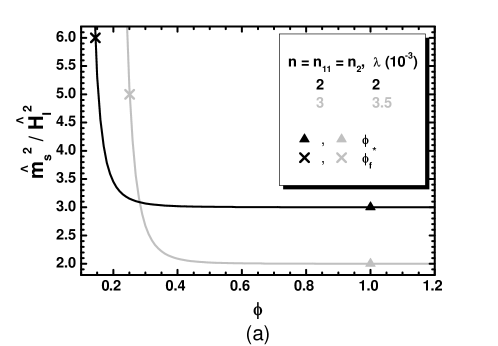
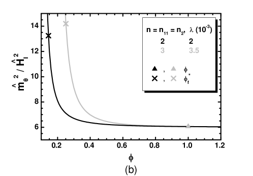
The most crucial output of our computation is the stabilization of $S$ (and $\theta$) during and after inflation. To highlight further this property, we present in \Freffig the variations of $\widehat{m}^{2}_{s}/\widehat{H}_{\rm I}^{2}$ and $\widehat{m}^{2}_{{\theta}}/\widehat{H}_{\rm I}^{2}$ as functions of $\phi$ for the inputs shown in the two last rows of \Treftab2, taking $n_{2}={\rm NewA}$ and $k=2$. It is evident that $\widehat{m}^{2}_{s}/\widehat{H}_{\rm I}^{2}$ and $\widehat{m}^{2}_{{\theta}}/\widehat{H}_{\rm I}^{2}$ remain larger than unity for $\phi_{\rm f}\leq\phi\leq\phi_{\star}$, where $\phi_{\star}$ and $\phi_{\rm f}$ are also depicted – the two $\phi_{\star}$’s are indistinguishable in Fig. 1-(b). For most $\phi$ values, $\widehat{m}^{2}_{s}/\widehat{H}_{\rm I}^{2}\simeq 2$ (light gray lines) or $3$ (black lines) for the no-scale or the IG model with a $\mathbb{Z}_{2}$ symmetry, respectively, whereas $\widehat{m}^{2}_{{\theta}}/\widehat{H}_{\rm I}^{2}\simeq 6$ for both cases. Note, finally, that both $\widehat{m}^{2}_{s}/\widehat{H}_{\rm I}^{2}$ and $\widehat{m}^{2}_{{\theta}}/\widehat{H}_{\rm I}^{2}$ are decreasing functions of $\phi$, and so if these are larger than unity for $\phi=\phi_{\star}$, they remain so for $\phi<\phi_{\star}$ too. This behavior is consistent with the formulae of Table 1, given that $f_{\phi}^{2}$ in the denominator of $\widehat{m}_{\chi^{\alpha}}^{2}$ decreases with $\phi$.

5 Conclusions

Refer to captionRefer to caption
Figure 1: The ratios $\widehat{m}^{2}_{s}/\widehat{H}_{\rm I}^{2}$ (a) and $\widehat{m}^{2}_{\theta}/\widehat{H}_{\rm I}^{2}$ (b) as functions of $\phi$ for $n=m={\rm NewA}=n_{2}=2$ and $\lambda=2\cdot 10^{-3}$ (black lines) or $m=2$, $n=n_{2}={\rm NewA}=3$ and $\lambda=3.5\cdot 10^{-3}$ (light gray lines). The values corresponding to $\phi_{\star}$ and $\phi_{\rm f}$ are also depicted.

We showed that Starobinsky-like inflation can be established in the context of SUGRA using the superpotential in \ErefWn and the Kähler potential in \ErefK3, which parameterizes the product space $SU(1,1)/U(1)\times SU(2)/U(1)$. Extending previous work [27, 28], based on induced gravity, we allow for the presence of different monomials (with exponents $n$ and $m$) of the inflaton superfield in $W$ and $K$. Observationally acceptable inflationary solutions are attained imposing the condition in \Erefcon2, which relates the exponents above with the curvature of the $SU(1,1)/U(1)$ space, $-2/{\rm NewA}$. As a consequence the inflationary predictions exhibit an attractor behavior depending exclusively on ${\rm NewA}$. Namely, we obtained $n_{\rm s}\simeq 0.965$ and $0.001\lesssim r\lesssim 0.005$ with negligible $a_{\rm s}$. Moreover, the mass of the inflaton turns out to be close to $1.25\cdot 10^{-5}$. The accompanying field $S$ is heavy enough and well stabilized during and after inflation, provided that the curvature of the $SU(2)/U(1)$ space is such that $0<n_{2}\leq 6$. Therefore, Starobinsky inflation realized within this SUGRA setting preserves its original predictive power. Furthermore it could be potentially embedded in string theory. If we adopt $c_{T}\gg 1$ and $n=m>1$, our models can be fixed if we impose two global symmetries – a continuous $R$ and a discrete $\mathbb{Z}_{n}$ symmetry – in conjunction with the requirement that the original inflaton takes subplanckian values. The one-loop radiative corrections remain subdominant and the corresponding effective theories can be trusted up to $m_{\rm P}$.

It is argued [35] that the models described by \ErefVhi1 for $n=m$ and $n_{21}=3$ develop one more attractor behavior towards the $(n_{\rm s},r)$’s encountered in the model of quadratic chaotic inflation. However, this result is achieved only for transplanckian inflaton values, without preserving the normalization of $A_{\rm s}$ in \ErefProb. For these reasons we did not pursue our investigation towards this direction. As a last remark, we would like to point out that the $S$-stabilization mechanism proposed in this paper has a much wider applicability. It can be employed to the models of ordinary [18] or kinetically modified [32, 37] non-minimal chaotic (and Higgs) inflation, without causing any essential alteration to their predictions. The necessary modifications are to split the relevant Kähler potential into two parts, replacing the $|S|^{2}$ depended part by the corresponding one included in $K_{3}$ – see \ErefK3 – and adjusting conveniently – as in \Erefcon2 – the prefactor of the logarithm including the inflaton in its argument. In those cases, though, it is not clear if the part of the Kähler potential for the inflaton sector parameterizes a symmetric Kähler manifold as in the case studied here.

Appendices

Appendix A Mathematical Supplement

In this Appendix we review some mathematical properties regarding the geometrical structure of the $SU(1,1)/U(1)\times SU(2)/U(1)$ Kähler manifold. For simplicity we present the case for which $c_{T}=n=m=1$ in Eqs. (3.16) and (2.8). The structure of the $SU(1,1)/U(1)$ coset space becomes more transparent if we define [14, 7]

$$T=\frac{1}{2}\frac{1-Z/\sqrt{{\rm NewA}}}{1+Z/\sqrt{{\rm NewA}}}\,\cdot$$ (A.1)

Upon the coordinate transformation above and a Kähler  transformation, the model described by the Kähler potential

$$\widetilde{K}_{3}=-{\rm NewA}\ln\left(1-\frac{|Z|^{2}}{{\rm NewA}}\right)+n_{2}\ln\left(1+\frac{|S|^{2}}{n_{2}}\right)$$ (A.2)

and the superpotential

$$\widetilde{W}=W(1+Z/\sqrt{{\rm NewA}})^{{\rm NewA}}$$ (A.3)

is equivalent to the model described by Eqs. (2.8) and (3.16). The Riemannian metric associated with $\widetilde{K}_{3}$ is given by

$$ds^{2}=g_{11}dZdZ^{*}+g_{2}dSdS^{*}\,,$$ (A.4)

having a diagonal structure with

$$g_{11}=\left(1-|Z|^{2}/{\rm NewA}\right)^{-2}\>\>\>\mbox{and}\>\>\>g_{2}=\left(1+|S|^{2}/n_{2}\right)^{-2}\,.$$ (A.5)

It is straightforward to show that the form of the line element in \Erefds remains invariant under the transformations

$$\frac{Z}{\sqrt{{\rm NewA}}}\rightarrow\frac{a_{1}Z/\sqrt{{\rm NewA}}+b_{1}}{b_{1}^{*}Z/\sqrt{{\rm NewA}}+a_{1}^{*}}\>\>\>\mbox{and}\>\>\>\frac{S}{\sqrt{n_{2}}}\rightarrow\frac{a_{2}S/\sqrt{n_{2}}+b_{2}}{-b_{2}^{*}S/\sqrt{n_{2}}+a_{2}^{*}}\,,$$ (A.6)

provided that $|a_{1}|^{2}-|b_{1}|^{2}=1$ and $|a_{2}|^{2}+|b_{2}|^{2}=1$. The Kähler potential $\widetilde{K}_{3}$ in \ErefK3t remains invariant under \Ereft12, up to a Kähler  transformation.

The transformations in \Ereft12 can be used to define transitive actions of the $2\times 2$ matrices

$$U_{1}=\mbox{ $\left\lgroup\begin{matrix}a_{1}&b_{1}\cr b_{1}^{*}&a_{1}^{*}\end{matrix}\right\rgroup$}\>\>\>\mbox{and}\>\>\>U_{2}=\mbox{ $\left\lgroup\begin{matrix}a_{2}&b_{2}\cr-b_{2}^{*}&a_{2}^{*}\end{matrix}\right\rgroup$}$$ (A.7)

on the scalar field manifolds parameterized by $Z$ and $S$ respectively. These matrices have the properties

$$U_{1}^{\dagger}\sigma_{3}U_{1}=\sigma_{3}\>\>\>\mbox{and}\>\>\>U_{2}^{\dagger}U_{2}=\leavevmode\hbox{\small 1\kern-3.8pt\normalsize 1}\>\>\>\mbox{with}\>\>\>\sigma_{3}={\sf diag}\left(1,-1\right)\>\>\>\mbox{and}\>\>\>\leavevmode\hbox{\small 1\kern-3.8pt\normalsize 1}={\sf diag}\left(1,1\right)\,,$$ (A.8)

and so, they provide representations of the $SU(1,1)$ and $SU(2)$ groups respectively. Now $U_{j}$ with $j=1,2$ can be written as $U_{j}=\widetilde{U}_{j}H_{j}$ (no summation over $j$ is applied), where the diagonal matrices $H_{j}={\sf diag}\left(e^{i{\theta}_{j}},e^{-i{\theta}_{j}}\right)$ stabilize the origins of the scalar field manifolds parameterized by $Z$ and $S$. Thus, the scalar field manifolds are isomorphic to the coset spaces $SU(1,1)/U(1)$ and $SU(2)/U(1)$. Notice that

$$\widetilde{U}_{1}=\mbox{ $\left\lgroup\begin{matrix}\alpha_{1}&c_{1}\cr c_{1}^{*}&\alpha_{1}\end{matrix}\right\rgroup$}\>\>\>\mbox{and}\>\>\>\widetilde{U}_{2}=\mbox{ $\left\lgroup\begin{matrix}\alpha_{2}&c_{2}\cr-c_{2}^{*}&\alpha_{2}\end{matrix}\right\rgroup$}$$ (A.9)

with $\alpha_{j}$ real and positive, $\alpha_{1}^{2}-|c_{1}|^{2}=1$ and $\alpha_{2}^{2}+|c_{2}|^{2}=1$. Therefore, $\widetilde{U}_{j}$ with $j=1$ and $2$ define equivalent parameterizations of the coset spaces $SU(1,1)/U(1)$ and $SU(2)/U(1)$ respectively.

Finally, applying the formula

$$R_{K}=g^{-3}\left(g_{,z}g_{,z^{*}}-gg_{,zz^{*}}\right)$$ (A.10)

for $g=g_{11}$ and $z=Z$ or $g=g_{2}$ and $z=S$, we find that the scalar curvatures of the spaces $SU(1,1)/U(1)$ and $SU(2)/U(1)$ are $-2/{\rm NewA}$ and $2/n_{2}$ respectively.

Appendix B The Effective Cut-off Scale

A characteristic feature of STI compared to conventional non-minimal chaotic inflation [18] is that perturbative unitarity is retained up to $m_{\rm P}$, despite the fact that its implementation with subplanckian $\phi$ values requires relatively large values of $c_{T}$ – see \Erefckmin. To show that this statement holds in the context of the generalization outlined in \Sreffhi, we extract the ultraviolet cut-off scale $\Lambda_{\rm UV}$ of the effective theory following the systematic approach of \crefriotto. We focus on the second term in the right-hand side of \ErefSaction1 for $\mu=\nu=0$ and ${\alpha}={\beta}=1$, and we expand it about $\langle{\phi}\rangle$, given by \Erefdphi, in terms of $\widehat{\delta\phi}$. Our result is written as

$$J^{2}\dot{\phi}^{2}\simeq\left(1-\frac{\sqrt{2{\rm NewA}}}{n}\widehat{\delta\phi}+\frac{3{\rm NewA}}{2n^{2}}\widehat{\delta\phi}^{2}-\frac{\sqrt{2}n^{3/2}_{11}}{n^{3}}\widehat{\delta\phi}^{3}+\cdots\right)\dot{}\widehat{\delta\phi}^{2},$$ (B.1a)
where we take into account \Erefcon2. Expanding similarly $\widehat{V}_{\rm I}$ in \ErefVhi2o we obtain
$$\widehat{V}_{\rm I}\simeq\frac{{\rm NewA}\lambda^{2}\widehat{\phi}^{2}}{2^{{\rm NewA}+1}c_{T}^{{\rm NewA}}}\left(1-\sqrt{\frac{{\rm NewA}}{2}}\frac{n+1}{n}\,\widehat{\delta\phi}+{\rm NewA}\left(1+n\right)\frac{11+7n}{24n^{2}}\,\widehat{\delta\phi}^{2}-\cdots\right).$$ (B.1b)

Since the coefficients in the series above are independent of $c_{T}$ and of order unity for reasonable $n$ and ${\rm NewA}$ values, we infer that our models do not face any problem with perturbative unitarity up to $m_{\rm P}$.

References

  • [1] P.A.R. Ade et al. [Planck Collaboration], \arxiv1502.02114.
  • [2] P.A.R. Ade et al. [Bicep2 and Planck Collaborations], Phys. Rev. Lett. 114, 101301 (2015) [\arxiv1502.00612].
  • [3] A.A. Starobinsky, Phys. Lett. B 91, 99 (1980).
  • [4] S.V. Ketov and A.A. Starobinsky, Phys. Rev. D 83, 063512 (2011) [\arxiv1011.0240];
    S.V. Ketov and N. Watanabe, J. Cosmology Astropart. Phys032011011 [\arxiv1101.0450];
    S.V. Ketov and A.A. Starobinsky, J. Cosmology Astropart. Phys082012022 [\arxiv1203.0805];
    S.V. Ketov and S. Tsujikawa, Phys. Rev. D 86, 023529 (2012) [\arxiv1205.2918];
    W. Buchmüller, V. Domcke and K. Kamada, Phys. Lett. B 726, 467 (2013) [\arxiv1306.3471];
    F. Farakos, A. Kehagias and A. Riotto, Nucl. Phys. B876 (2013) 187 [\arxiv1307.1137];
    J. Alexandre, N. Houston and N.E. Mavromatos, Phys. Rev. D 89, 027703 (2014) [\arxiv1312.5197];
    K. Kamada and J. Yokoyama, Phys. Rev. D 90, 103520 (2014) [\arxiv1405.6732];
    R. Blumenhagen et al., Phys. Lett. B 746, 217 (2015) [\arxiv1503.01607];
    T. Li, Z. Li and D.V. Nanopoulos, J. High Energy Phys. 10, 138 (2015) [\arxiv1507.04687];
    S. Basilakos, N.E. Mavromatos and J. Sola, \arxiv1505.04434.
  • [5] J. Ellis, D.V. Nanopoulos and K.A. Olive, Phys. Rev. Lett.  111, 111301 (2013);
    Erratum-ibid.  111, no. 12, 129902 (2013) [\arxiv1305.1247].
  • [6] J. Ellis, H.J. He and Z.Z. Xianyu, Phys. Rev. D 91, no. 2, 021302 (2015) [\arxiv1411.5537];
    I. Garg and S. Mohanty, Phys. Lett. B 751, 7 (2015) [\arxiv1504.07725].
  • [7] J. Ellis D. Nanopoulos and K. Olive, J. Cosmology Astropart. Phys102013009 [\arxiv1307.3537].
  • [8] R. Kallosh and A. Linde, J. Cosmology Astropart. Phys062013028 [\arxiv1306.3214].
  • [9] D. Roest, M. Scalisi and I. Zavala, J. Cosmology Astropart. Phys112013007 [\arxiv1307.4343].
  • [10] C. Pallis, J. Cosmology Astropart. Phys042014024 [\arxiv1312.3623].
  • [11] A.B. Lahanas and K. Tamvakis, Phys. Rev. D 91, no. 8, 085001 (2015) [\arxiv1501.06547].
  • [12] R. Kallosh, A. Linde and T. Rube, Phys. Rev. D 83, 043507 (2011) [\arxiv1011.5945].
  • [13] E. Cremmer, S. Ferrara, C. Kounnas and D.V. Nanopoulos, Phys. Lett. B 133, 61 (1983);
    J.R. Ellis, A.B. Lahanas, D.V. Nanopoulos and K. Tamvakis, Phys. Lett. B 134, 429 (1984).
  • [14] A.B. Lahanas and D.V. Nanopoulos, Phys. Rept. 145, 198 (1987).
  • [15] T. Terada, Y. Watanabe, Y. Yamada and J. Yokoyama, J. High Energy Phys. 02, 105 (2015) [\arxiv1411.6746].
  • [16] J. Ellis, M. Garcia, D. Nanopoulos and K. Olive, J. Cosmology Astropart. Phys102015003 [\arxiv1503.08867].
  • [17] H.M. Lee, J. Cosmology Astropart. Phys082010003 [\arxiv1005.2735].
  • [18] M.B. Einhorn and D.R.T. Jones, J. High Energy Phys. 03, 026 (2010) [\arxiv0912.2718];
    S. Ferrara et al., Phys. Rev. D 83, 025008 (2011) [\arxiv1008.2942];
    C. Pallis and N. Toumbas, J. Cosmology Astropart. Phys022011019 [\arxiv1101.0325];
    C. Pallis and N. Toumbas, J. Cosmology Astropart. Phys122011002 [\arxiv1108.1771];
    C. Pallis and Q. Shafi, Phys. Rev. D 86, 023523 (2012) [\arxiv1204.0252].
  • [19] C. Kounnas, D. Lüst and N. Toumbas, Fortsch. Phys. 63, 12 (2015) [\arxiv1409.7076].
  • [20] C. Pallis, PoS CORFU2012 (2013) 061 [\arxiv1307.7815].
  • [21] I. Antoniadis, E. Dudas, S. Ferrara and A. Sagnotti, Phys. Lett. B 733, 32 (2014) [\arxiv1403.3269].
  • [22] D. Baumann and L. McAllister, \arxiv1404.2601.
  • [23] S. Kachru et al., J. Cosmology Astropart. Phys102003013 [\hepth0308055].
  • [24] O. DeWolfe and S.B. Giddings, Phys. Rev. D 67, 066008 (2003) [\hepth0208123].
  • [25] D.S. Salopek, J.R. Bond and J.M. Bardeen, Phys. Rev. D 40, 1753 (1989);
    R. Fakir and W.G. Unruh, Phys. Rev. D 41, 1792 (1990).
  • [26] G.F. Giudice and H.M. Lee, Phys. Lett. B 733, 58 (2014) [\arxiv1402.2129].
  • [27] R. Kallosh, Phys. Rev. D 89, no. 8, 087703 (2014) [\arxiv1402.3286].
  • [28] C. Pallis, J. Cosmology Astropart. Phys082014057 [\arxiv1403.5486].
  • [29] A. Kehagias, A.M. Dizgah, and A. Riotto, Phys. Rev. D 89, 043527 (2014) [\arxiv1312.1155].
  • [30] S. Cecotti, Phys. Lett. B 190, 86 (1987).
  • [31] C. Pallis, J. Cosmology Astropart. Phys102014058 [\arxiv1407.8522];
    C. Pallis and Q. Shafi, J. Cosmology Astropart. Phys032015023 [\arxiv1412.3757];
    C. Pallis, PoS CORFU 2014, 156 (2015) [\arxiv1506.03731].
  • [32] G. Lazarides and C. Pallis, J. High Energy Phys. 11, 114 (2015) [\arxiv1508.06682].
  • [33] J. Ellis et al., J. Cosmology Astropart. Phys012015010 [\arxiv1409.8197];
    C. van de Bruck and L.E. Paduraru, Phys. Rev. D 92, no. 8, 083513 (2015) [\arxiv1505.01727];
    S. Kaneda and S.V. Ketov, Eur. Phys. J. C 76, no. 1, 26 (2016) [\arxiv1510.03524];
    G.K. Chakravarty, S. Das, G. Lambiase and S. Mohanty, \arxiv1511.03121.
  • [34] S. Renaux-Petel and K. Turzynski, \arxiv1510.01281.
  • [35] R. Kallosh, A. Linde and D. Roest, J. High Energy Phys. 09, 062 (2014) [\arxiv1407.4471];
    B. Mosk and J.P. van der Schaar, J. Cosmology Astropart. Phys122014022 [\arxiv1407.4686].
  • [36] A. Hindawi, B.A. Ovrut and D. Waldram, Nucl. Phys. B476, 175 (1996) [\hepth9511223];
    I. Dalianis et al., J. High Energy Phys. 01, 043 (2015) [\arxiv1409.8299].
  • [37] C. Pallis, Phys. Rev. D 91, no. 12, 123508 (2015) [\arxiv1503.05887];
    C. Pallis, PoS PLANCK 2015, 095 (2015) [\arxiv1510.02306];
    C. Pallis, Phys. Rev. D 92, no. 12, 121305(R) (2015) [\arxiv1511.01456].
  • [38]