Inspiralling, Non-Precessing, Spinning Black Hole Binary Spacetime
via Asymptotic Matching

Abstract

We construct a new global, fully analytic, approximate spacetime which accurately describes the dynamics of non-precessing, spinning black hole binaries during the inspiral phase of the relativistic merger process. This approximate solution of the vacuum Einstein’s equations can be obtained by asymptotically matching perturbed Kerr solutions near the two black holes to a post-Newtonian metric valid far from the two black holes. This metric is then matched to a post-Minkowskian metric even farther out in the wave zone. The procedure of asymptotic matching is generalized to be valid on all spatial hypersurfaces, instead of a small group of initial hypersurfaces discussed in previous works. This metric is well suited for long term dynamical simulations of spinning black hole binary spacetimes prior to merger, such as studies of circumbinary gas accretion which requires hundreds of binary orbits.

I INTRODUCTION

The recent announcement of GW150914 Abbott et al. (2016a) from the Laser Interferometer Gravitational wave Observatory (LIGO) Abbott et al. (2009) has provided the first strong evidence of a black hole binary (BHB) coalescence due to the emission of gravitational waves (GWs). This discovery kicks off the era of gravitational wave astronomy, and provides further justification to the study of the inspiral and merger of BHBs. The merger of stellar-mass black holes (BHs), such as GW150914 and other BHB potential LIGO sources, are not expected to have any electromagnetic (EM) counterparts Abbott et al. (2016b). However, Ref. Connaughton et al. (2016) reported a potential $\gamma$-ray EM counterpart observed by the Gamma-Ray Burst Monitor Meegan et al. (2009) on Fermi which is consistent with the sky localization of GW150914.

The existence of supermassive BHs residing in the centers of galaxies Gültekin et al. (2009) indicates another type of possible BHB, one for which EM counterparts are not only possible, but are also frequent. Galaxies will undergo mergers of both stars and gas as the Universe evolves Frenk et al. (1985); Bardeen et al. (1986). In the process of the galactic merger, the supermassive BHs will form a bound pair due to torques exerted by the surrounding gas and stars, dynamical friction, and gravitational slingshots that eject stars from the nucleus of the merging system. Gravitational radiation becomes the dominant energy loss mechanism as the BHBs become closely separated, eventually driving the two BHs to the full merger. The consequences for galactic evolution of these mergers are very deep, as strong correlations between galactic structure and central BH mass indicate tight feedback between BH and galaxy growth.

Future space-based GW missions, like the proposed European New Gravitational wave Observatory (NGO) Amaro-Seoane et al. (2013a, 2012, b) and the DECi-hertz Interferometer Gravitational wave Observatory (DECIGO) Seto et al. (2001), will be sensitive to such events, but are decades away from launch. Fortunately, in the case of supermassive BHBs, highly-relativistic magnetized gas could flow around the pair, as well as around each BH companion. Therefore, powerful EM signals should accompany the inspiral and merger of BHBs Roedig et al. (2014); Schnittman (2013).

The main research focus of the authors is to simulate the effects of spinning supermassive BHB mergers on nearby gas in sufficient detail to enable EM observations of these events. This paper represents a major step forward in achieving this goal by providing an analytic spacetime that can handle spinning BHBs. Since 2005 Pretorius (2005); Campanelli et al. (2006a); Baker et al. (2006), a handful of numerical relativity simulations of BHBs have been successfully carried on for nearly a hundred orbits Lousto and Healy (2015a); Szilagyi et al. (2015), providing the necessary waveforms for current and future GW detectors Aasi et al. (2014); Mroue et al. (2013).

However, in the case of BHBs in a gaseous environment, numerical magnetohydrodynamic (MHD) simulations are still very expensive to carry out Bode et al. (2010, 2012); Pahari and Pal (2010); Farris et al. (2010, 2011, 2012, 2014, 2015); Giacomazzo et al. (2012); Gold et al. (2013, 2014). This is because we need to resolve turbulences and shocks in the gas, as well as secular variations in the circumbinary disk on the time scale of hundreds to thousands of binary orbits (see Ref. Noble et al. (2012) for detailed discussion). In order to make long-term and accurate MHD simulations possible, we developed a complementary analytic approach to treat dynamical, nonspinning, BHB spacetimes Noble et al. (2012); Mundim et al. (2014); Zilhao et al. (2015); Zilhão and Noble (2014). This spacetime is a solution to the Einstein field equations in the approximation that the BHB is slowly inspiralling to merger. In this situation, gravity is weak [$r_{g}/r=GM/(rc^{2})\ll 1$] and motions are slow [$v/c\ll 1$], so the post-Newtonian (PN) approximation is a very good description of spacetime. Using a spacetime accurate to 2.5PN order (i.e., including terms up to $\sim(r_{g}/r)^{5/2}$), and using the 3.5PN equations of motion (EOM) to describe the GW driven inspiral of the orbital evolution Blanchet (2014), we demonstrated that circumbinary disks can track a supermassive BHB for hundreds of orbits until the binary practically reaches the relativistic merger regime Noble et al. (2012).

In a more recent paper Mundim et al. (2014), we extended the metric all the way down to the horizons of each BH. We did this by broadening the framework introduced in Refs. Yunes et al. (2006); Yunes and Tichy (2006); Johnson-McDaniel et al. (2009) for constructing a spacetime metric valid for initial data, to a full dynamical spacetime metric valid for arbitrary times. This metric is constructed by stitching together different spacetime metrics valid in different regions of the full BHB spacetime (see II). We extend this framework here to include the effects of spinning BHs.

There are important spin-based effects which affect the dynamics of the BHB that can also significantly alter the dynamic of the surrounding gas. The mechanisms associated with accretion at larger separations may drive the spins into alignment with both the binary orbital axis and the circumbinary disk axis Bogdanovic et al. (2007); Miller and Krolik (2013); Sorathia et al. (2013). In this case, another mechanism due to spin-orbit coupling can delay or prompts the merger of the BHB according to the sign of the spin-orbit coupling Campanelli et al. (2006b). This could have a significant effect on the total pre-merger light output and its time-dependence.

At closer BHB separations, little is know about the effectiveness of these accretion driven spin-alignment mechanisms. In this situation, spin-spin and spin-orbit interactions can also cause the spins to precess, leading to time-dependence in non-planar gas orbits Campanelli et al. (2006). Gravitomagnetic torques arising from the BH spins oblique to the orbital axis may then push the accretion streams onto the BHs out of the orbital plane and alter the tidal limitation of the mini-disks, particularly for relatively small binary separations. Another interesting spin effect is the recently discovered spin-flip-flop phenomenon Lousto and Healy (2015a, b), where the spin of one of the BHs completely reverses. This may cause the gas in the neighborhood of the binary to be continually disturbed in a manner that will produce a very distinct EM signature from the disk. Finally, highly spinning BHBs may recoil at thousands of km/s Campanelli et al. (2007a, b); Koppitz et al. (2007); González et al. (2007) due to asymmetrical emission of gravitational radiation induced by the BH spins Lousto et al. (2012); Lousto and Zlochower (2011). The resulting ejected BH may carry along part of the original accretion disk causing it to be bright enough to be observable (see Komossa (2012) for a review).

In this paper, we generalize Mundim et al. (2014) to spinning BHBs, with spins aligned and counteraligned with the orbital angular momentum of the binary, in a quasi circular inspiral. We will address the case of oblique spins and spin precession Thorne and Hartle (1985) in future work Nakano et al. . Our new spinning global metric must, of course, approximately satisfy the Einstein equations, if it is to be considered a true spacetime metric representing a BHB. For each zone, we check the validity of the spacetime analytically in the black hole perturbation, the PN and the post-Minkowski (PM) approximations by computing the deviations from Einstein’s equations. We can construct several curvature invariants to determine the overall accuracy of the approximations. One such invariant is the Ricci scalar, which can be compared against the exact vacuum solution quantity of $R=0$. Another quantity is the Hamiltonian constraint, which is used in the numerical relativity community to measure the amount of “fake” mass in the system caused by violations to the Einstein vacuum field equations. Finally, we introduce an invariant quantity related to the Kretschmann invariant $R_{\mu\nu\rho\delta}R^{\mu\nu\rho\delta}$, which has the benefit of being a normalized measure of the violation of the global metric to the Einstein equations.

This paper is organized as follows. Sec. II outlines the different approximate metrics, and details of their construction and matching to obtain the global metric. Sec. III discusses the numerical analysis of this global metric by the calculation of several spacetime invariants that impress upon us the validity of the global metric. Finally, Sec. IV contains useful discussion, conclusions, and future work. The appendices A, B, C and D describe the choice of transition functions that are utilized in the global metric, the details of the ingoing Kerr to Cook-Scheel coordinate transformation, the innermost stable circular orbit (ISCO) and an effective evaluation of the inner zone metric.

Throughout this paper, we follow the notation of Misner, Thorne and Wheeler Misner et al. (1973), specifically, greek letters ($\alpha,\beta,\gamma,\cdot\cdot\cdot$) used as indices are indicative of spacetime coordinates, and latin letters ($i,j,k,\cdot\cdot\cdot$) are used in discussions of spatial coordinates only. The covariant metric is then written as $g_{\mu\nu}$, and has a signature of $(-,+,+,+)$. We use the geometric unit system, where $G=c=1$, with the useful conversion factor $1M_{\odot}=1.477\;{\rm{km}}=4.926\times 10^{-6}\;{\rm{s}}$.

II CONSTRUCTION OF APPROXIMATE GLOBAL METRIC

We are concerned with the construction of the approximate global metric with spin for a BHB pair on a quasi circular inspiral, in the inspiral regime. To find this global metric for the BHBs, we first consider the individual regions where different approximations and assumptions hold (see Table 1); the inner zone (IZ) around BH1 (IZ1) and around BH2 (IZ2), the near zone (NZ) around the two BHs, and the far zone (FZ) or wave zone farthest out.

Table 1: Regions of validity for the different zones and BZ locations. Here $r_{1}$ and $r_{2}$ are the distances from the first or second BH with mass $m_{1}$ or $m_{2}$, $r$ is the distance from the center of mass to a field point, $r_{12}$ is the orbital separation, and $\lambda$ is the gravitational wavelength. For BZs to exist, the system must satisfy $m_{1,2}\ll r_{12}$, though we expect that the metric will break down before this condition is violated. (This was also presented in Refs. Gallouin et al. (2012); Mundim et al. (2014); Zlochower et al. (2015).)

Zone	Region of Validity
IZ1	$0$	$<$	$r_{1}$	$\ll$	$r_{12}$
IZ2	$0$	$<$	$r_{2}$	$\ll$	$r_{12}$
NZ	$m_{A}$	$\ll$	$r_{A}$	$\ll$	$\lambda$
FZ	$r_{12}$	$\ll$	$r$	$<$	$\infty$
IZ1-NZ BZ	$m_{1}$	$\ll$	$r_{1}$	$\ll$	$r_{12}$
IZ2-NZ BZ	$m_{2}$	$\ll$	$r_{2}$	$\ll$	$r_{12}$
NZ-FZ BZ	$r_{12}$	$\ll$	$r$	$\ll$	$\lambda$

II.1 Subdividing spacetime

In the inner region very close to the individual BHs, we treat the spacetime as a vacuum Kerr solution with linear perturbations as in Ref. Yunes and González (2006). The PN metric subdivision that was briefly discussed above is known as the NZ. This metric is valid in the slow motion, weak field limit. The addition of spins to the NZ will add terms to the PN expansion which, to lowest order, are the 1.5PN  leading order spin-orbit coupling and 2PN leading order spin-spin terms. The NZ is defined to be valid in a region far away from the individual BHs (to not violate the weak field approximation), but not farther away than a gravitational wavelength ($\lambda\sim 2\pi/\omega_{\rm GW}\sim\pi/\omega_{\rm orb}\sim\pi(r_{12}^{3}/M)^{1/2}$, where $M=m_{1}+m_{2}$ is the total mass) from the center of mass of the binary system. The region even farther out than a gravitational wavelength from the center of mass can be described as the FZ, in which the metric takes the form of flat (Minkowski) space, with outgoing GWs perturbing the spacetime. The FZ is modeled with a PM (or multipolar) formalism Will and Wiseman (1996). Unlike in PN formalism, PM expansions correctly treat the retardation of the gravitational field, which is essential for understanding the FZ. This subdivision of the spacetime into different regions will only be valid as long as the slow motion approximation holds, and will break down around an orbital separation $r_{12}\approx 10M$ Yunes and Berti (2008); Zhang et al. (2011).

Once we have the individual metrics for the different zones, we need to stitch them all together into a global metric, asymptotically matching the IZ, NZ, and FZ to each other in BZs. The procedure of matching adjacent metrics to one another requires the metrics to be in the same coordinate system. In other words, one of the metrics (and its parameters) will be related to the next door metric via some coordinate transformations, constructed such that the transformed metric asymptotes to the adjacent metric in the BZ. Asymptotic matching in GR has been successfully done in Refs. Yunes et al. (2006); Alvi (2000); Pati and Will (2002); Alvi (2003); Yunes and Tichy (2006); Yunes (2007); Johnson-McDaniel et al. (2009); Gallouin et al. (2012), but in all of these papers, the authors asymptotically matched in the context of initial data for BHB simulations, which implies that their focuses were on a particular spatial hypersurface. However, in the context of this work, this restriction must be lifted if there is to be any hope of dynamic, long time evolutions of BHBs. Ref. Mundim et al. (2014) successfully removed this restriction in the context of nonspinning BHs. The task now is to do this in the context of spinning BHs. The extension to spinning BHs should be more astrophysically relevant than the non spinning BHB case covered in Ref. Mundim et al. (2014), because it is thought that most astrophysical BHs have spin Bardeen (1970).

Once the metrics have been asymptotically matched, we construct a global metric by introducing transition functions that take us from one metric to the next in the BZs without introducing artificial errors Yunes (2007) into the metric that are larger than the errors already incurred in the approximations used in construction of the individual metrics.

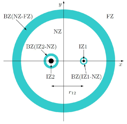
Figure 1: A schematic diagram detailing the different zones for the approximate analytic spacetime looking down the $z$-axis at a particular instant in time. The black dots on the $x$-axis represent the two BHs, with an orbital separation of $r_{12}$. The cyan shells indicate the BZs – regions where two adjacent metrics have overlapping regions of validity. The outermost shell is the NZ-FZ BZ, with both the IZ1-NZ and IZ2-NZ BZs labeled around the individual BHs. The IZ, NZ, and FZ are denoted as the regions contained by the BZs. Note that the circular nature of the BZs is not physical, only schematic, and in general it is expected that they will have some distortions. (This was also presented in Refs. Gallouin et al. (2012); Mundim et al. (2014); Zlochower et al. (2015).)

The different zones and their associated BZs are summarized in Fig. 1 and Table 1. The cyan shells indicate the BZs between the individual subdivided metrics, where both of the adjacent metrics are valid. We note that the figure is purely schematic; in general, there is no inherent symmetry that would cause the BZs to be like the spherical shells depicted, so in reality these BZs would be distorted. It is in these BZs that asymptotic matching of the individual metrics takes place. Finally, the resulting matched metrics are stitched together with the proper transition functions satisfying the Frankenstein theorems Yunes (2007), yielding a global analytic approximate spacetime. The construction of the asymptotically matched global metric has been calculated in Ref. Gallouin et al. (2012), but only in the context of initial data and not for long time evolutions of the BHB system.

II.2 Inner Zone

The IZs in Fig. 1 and Table 1 are constructed following the work laid out in Ref. Yunes and González (2006), and applied to BHB initial data on a single spatial hypersurface in Ref. Gallouin et al. (2012). The IZ metric is approximately described by the Kerr metric $g_{\mu\nu}^{\rm Kerr}$ plus a linearized vacuum perturbation $h_{\mu\nu}^{\rm IZ}$:

$$g_{\mu\nu}^{\rm IZ}=g_{\mu\nu}^{\rm Kerr}+h_{\mu\nu}^{\rm IZ}\,.$$ (1)

Here the Kerr metric is given by the mass of the Kerr BH $m_{\rm Kerr}$, and the dimensional spin parameter $a$, which can be related to the dimensionless spin parameter $\chi$ by $a=\chi m_{\rm Kerr}$ and the dimensional spin $S=\chi m_{\rm Kerr}^{2}$. It is convenient to work with $\chi$ in our calculations because it is a normalized quantity ($0\leq|\chi|\leq 1$), with zero being a non spinning (Schwarzschild) BH, and one being a maximally spinning Kerr BH.

The metric perturbation $h_{\mu\nu}^{\rm IZ}$ has been studied and applied for Schwarzschild BHs, where we can use the Regge-Wheeler-Zerilli-Moncrief formalism Regge and Wheeler (1957); Zerilli (1970); Moncrief (1974); Nagar and Rezzolla (2005), which is generally valid for static spherically symmetric spacetimes. However, when looking at the case of the Kerr background, this formalism is not applicable, because Kerr is not spherically symmetric, and so there is not a multipole decomposition of metric perturbations, and the Einstein equations cannot be uncoupled into wave equations. A reformulation due to Newman and Penrose Newman and Penrose (1962) (from here out referred to as the NP formalism) of the Einstein equations and Bianchi identities projected along a null tetrad coinciding with the null symmetries of the spacetime (Kerr BHs are a type D algebraically special solution) allowed Teukolsky Teukolsky (1973) to write down a single master wave equation for the perturbations of Kerr in terms of the Weyl scalars (constructed from contracting the Weyl tensor with the same conveniently chosen null tetrad, called the Kinnersley tetrad) $\psi_{0}$ or $\psi_{4}$. Solutions to the Teukolsky equation yield the perturbed Weyl scalars.

To obtain the metric perturbation from the Weyl scalar, we must use the Chrzanowski procedure Chrzanowski (1975), which takes the Weyl scalar $\psi_{0}$ and acts a differential operator on it to yield a valid metric perturbation. This was later amended by Wald Wald (1978), and Kegles and Cohen Kegeles and Cohen (1979) to use a Hertz potential $\Psi$ instead of a Weyl scalar ($\psi_{0}$ for ingoing radiation, suitable for studying perturbations, or $\psi_{4}$ for outgoing radiation, suitable for GW studies Campanelli and Lousto (1999)). A brief description of the metric perturbation construction via the Chrzanowski procedure is summarized in the following.

The metric perturbation $h_{\mu\nu}$ is constructed via the Chrzanowski procedure by applying a certain differential operator to the so-called Hertz potential. The Hertz potential must satisfy a certain differential equation with a source given by the NP scalar $\psi_{0}$, and the differential equation can be inverted to yield the potential $\Psi$ totally in terms of $\psi_{0}$ Wald (1978); Ori (2003). Therefore, the construction of the metric perturbation $h_{\mu\nu}$ boils down to finding an appropriate solution for the NP scalar $\psi_{0}$. The metric perturbation is in the ingoing radiation gauge, given by the perturbation contracted along the tetrad components, $h_{\ell\ell}=h_{\ell n}=h_{\ell m}=h_{\ell\overline{m}}=h_{m\overline{m}}=0$ where $\ell_{\mu}$ and $m_{\mu}$ are components of the Kinnersley null tetrad, and $\overline{m}_{\mu}$ is the complex conjugate of $m_{\mu}$.

This NP scalar must, of course, satisfy the Teukolsky equation Teukolsky (1973). However, when the external universe (the source of the perturbation) is slowly-varying (as is the case of most interest to this work, when the external universe is a second BH on a quasi-circular inspiral with a large separation), it is possible to solve this equation perturbatively Yunes and González (2006). Thus, we can write $\psi_{0}$ in terms of the spin-2 weighted spherical harmonics ${}_{2}Y_{lm}$ as

$$\psi_{0}=\sum_{\ell,m}R_{\ell m}(r)z_{\ell m}(v)\;{}_{2}Y_{\ell m}(\theta,\phi)\,,$$ (2)

where the radial and time dependence are product decomposed into terms of unknown real functions $R_{\ell m}(r)$, and complex functions $z_{\ell m}(v)$. Here, $v$ is the advanced Kerr-Schild time coordinate. $z_{\ell m}$ can be written in terms of electric and magnetic tidal tensors, which to leading order in BH perturbation theory Poisson (2004) can be truncated at the $\ell=2$ quadrupolar deformation. The radial functions $R_{\ell m}$ must then satisfy the (time-independent) Teukolsky equation, and can be solved in terms of hypergeometric functions. Solving the time-independent Teukolsky equation implies that the $z_{\ell m}$ functions are slowly varying or constant in time. This can then be reconstructed into a functional form for $\psi_{0}$.

With this NP scalar under control, it is possible to compute the Hertz potential, and from that, the full metric perturbation $h_{\mu\nu}$. Ref. Yunes and González (2006) provides the full form of $h_{\mu\nu}$ in Eddington-Finkelstein (ingoing Kerr) coordinates.

The final form of the IZ metric needs to have several desirable features to be of use. One of which is horizon penetrating, Cook-Scheel harmonic (CS-H) coordinates ($T,\,X,\,Y,\,Z$) Cook and Scheel (1997). The details of taking the IZ from the IK coordinates to the more useful CS-H coordinates is left to Appendix B. From the CS-H coordinates, it is simply a matter of applying yet another transformation to take the metric from the IZ coordinates to the coordinates used in the NZ, the PN harmonic (PNH) coordinates.

II.3 Near Zone

The NZ in Fig. 1 and Table 1 is the region sufficiently distant from either BH that the metric can be described through the PN metric:

$$g_{\mu\nu}^{\rm NZ}=\eta_{\mu\nu}+h_{\mu\nu}^{\rm NZ}\,,$$ (3)

where $\eta_{\mu\nu}$ is the Minkowski (flat space) metric, and $h_{\mu\nu}$ is a PN metric perturbation Gallouin et al. (2012). In the PN approximation, the Einstein equations are solved in an expansion of both $v/c\ll 1$ (slow motion) and $GM/(Rc^{2})\ll 1$ (weak fields), where $M$ is the total mass of the BHs, $R$ is the orbital separation ($r_{12}$) or the center of mass to one BH ($r_{1,2}$), and the $G$’s and $c$’s have been replaced for convenience. By construction, the PN approximation models the BHs as point particles.

The metric perturbation we use is specified in Ref. Blanchet et al. (1998) for the spin independent terms and the first non-vanishing spin terms are outlined in Refs. Tagoshi et al. (2001); Faye et al. (2006), giving us a 1.5PN metric in PNH coordinates (which are a Cartesian-like, rectangular coordinate system) to match the IZ to as

$$g_{00}^{\rm NZ}+1= \frac{2m_{1}}{r_{1}}+\frac{m_{1}}{r_{1}}\left[4\mathbf{v}_{1}^{2}-(\mathbf{n}_{1}\cdot\mathbf{v}_{1})^{2}\right]-2\frac{m_{1}^{2}}{r_{1}^{2}}$$ (4)

$$-m_{1}m_{2}\Biggl{[}\frac{2}{r_{1}r_{2}}+\frac{r_{1}}{2r_{12}^{3}}-\frac{r_{1}^{2}}{2r_{2}r_{12}^{3}}+\frac{5}{2r_{2}r_{12}}\Biggr{]}$$ (5)

$$+\frac{4m_{1}m_{2}}{3r_{12}^{2}}(\mathbf{n}_{12}\cdot\mathbf{v}_{12})$$ (6)

$$+\frac{4}{r_{1}^{2}}\epsilon_{ijk}v_{1}^{i}s_{1}^{j}n_{1}^{k}+(1\leftrightarrow 2)+{\cal{O}}(v^{6})\,,$$ (7)

$$g_{0i}^{\rm NZ}= -\frac{4m_{1}}{r_{1}}v_{1}^{i}-\frac{2}{r_{1}^{2}}\epsilon_{ijk}s_{1}^{j}n_{1}^{k}+(1\leftrightarrow 2)+{\cal{O}}(v^{5})\,,$$ (8)

$$g_{ij}^{\rm NZ}-\delta_{ij}= \frac{2m_{1}}{r_{1}}\delta_{ij}+(1\leftrightarrow 2)+{\cal{O}}(v^{4})\,,$$ (9)

where $m_{A}$, $s_{A}^{i}$, $y_{A}^{i}$ and $v_{A}^{i}$ denote the mass, spin angular momentum, location and velocity of the $A$th PN particle, respectively. Other notations that have been introduced above are $r_{12}=|\mathbf{y}_{1}-\mathbf{y}_{2}|$, $\mathbf{n}_{12}=(\mathbf{y}_{1}-\mathbf{y}_{2})/b$, $\mathbf{v}_{12}=\mathbf{v}_{1}-\mathbf{v}_{2}$, $r_{A}=|\mathbf{x}-\mathbf{y}_{A}|$, $n_{A}^{i}=(x^{i}-y_{A}^{i})/r_{A}$ and $\epsilon_{ijk}$ is the Levi-Civita symbol.

In practice, we use higher order PN EOM than is strictly allowed by matching. Since the IZ metric is a first order BH perturbation theory, we cannot use any higher order than linear for the NZ metric in the matching calculation. We can, however, use a higher order PN EOM outside of the matching to have more accurate PN dynamics in the NZ for long time evolutions of BHB systems. The higher order formulas are summarized in the appendix of Ref. Ajith et al. (2012), and also in Ref. Blanchet (2014) (see also Sec. III.6). More specifically, we may use the energy function in Eq. (A.11), flux function in Eq. (A.13), and mass loss in Eq. (A.14) given in Ref. Ajith et al. (2007) and follow the procedure to derive the orbital phase evolution presented in Sec. 9.3 of Ref. Blanchet (2014). This gives the aligned spinning version of Eq. (317) in Ref. Blanchet (2014) which is for the nonspinning case.

II.4 Asymptotic Matching

The IZ metric is described by the CS-H coordinates $X^{\alpha}$ and the parameters $\Lambda^{\alpha}=(m_{\rm Kerr},\,a,\,z_{R,m},\,z_{I,m})$, where $z_{R,m}$ and $z_{I,m}$ are the real and imaginary parts of $z_{2m}$ respectively. On the other hand, the NZ metric is written in PNH coordinates $x^{\alpha}$ with the parameters $\lambda^{\alpha}=(m_{1},\,m_{2},\,b,\,s_{1}^{i},\,s_{2}^{i})$. We require that these two expressions be diffeomorphic to each other, leading us to a set of equations that relate the coordinates of the two metrics

$$g^{\rm NZ}_{\alpha\beta}=\frac{\partial X^{\gamma}}{\partial x_{\alpha}}\frac{\partial X^{\delta}}{\partial x_{\beta}}g^{\rm IZ}_{\gamma\delta}\,,$$ (10)

and expressions that relate the parameters used in each zone. We consider $b=r_{12}$ a constant in the matching calculation here and recover the time dependence in the final expression.

In the BZ in Fig. 1 and Table 1, we use series expansions with respect to $(m_{2}/b)^{1/2}={\cal{O}}(v)$. The IZ coordinates and parameters are expanded as

$$X^{\alpha}\left(x^{\beta}\right)= \sum_{i=0}^{n}\left(\frac{m_{2}}{b}\right)^{i/2}\left(X^{\alpha}\right)_{i}\left(x^{\beta}\right)+{\cal{O}}(v^{n+1})\,,$$

$$\Lambda^{\alpha}\left(\lambda^{\beta}\right)= \sum_{i=0}^{n}\left(\frac{m_{2}}{b}\right)^{i/2}\left(\Lambda^{\alpha}\right)_{i}\left(\lambda^{\beta}\right)+{\cal{O}}(v^{n+1})\,,$$ (11)

where $(X^{\alpha})_{i}$ and $(\Lambda^{\alpha})_{i}$ denote $i$th expansion functions of the NZ coordinates $x^{\beta}$ and those of the NZ parameters $\lambda^{\beta}$, respectively.

In the asymptotic matching between the IZ1 and NZ metrics to $O[(m_{2}/b)^{1}]$, i.e., $n=2$ in the above equations, we have already discussed in Ref. Gallouin et al. (2012) that the non-spinning matching transformation is sufficient, even if we consider the matching of the spinning case. This is because the spinning body effect arises from the $n=3$ matching. Obtaining the mass $m_{\rm Kerr}=m_{1}$ (also the dimensional spin parameter $a=s_{1}^{z}/m_{1}$ for non-precessing, spinning BHBs), the quadrupolar field is

$$z_{R,0} =\frac{2m_{2}}{b^{3}}\,,$$ (12)

$$z_{R,2} =\frac{6m_{2}}{b^{3}}\cos 2\omega t\,,\quad z_{R,-2}=\frac{6m_{2}}{b^{3}}\cos 2\omega t\,,$$ (13)

$$z_{I,2} =-\frac{6m_{2}}{b^{3}}\sin 2\omega t\,,\quad z_{I,-2}=\frac{6m_{2}}{b^{3}}\sin 2\omega t\,,$$ (14)

where $\omega\sim\sqrt{M/b^{3}}$ to lowest PN order, and the other components vanish.

II.5 Expansion of the Nonspinning Part of the IZ and NZ Metrics

Using $m_{1}\ll r_{1}\ll b$ in the BZ in Fig. 1 and Table 1, we expand the NZ and IZ metrics. First, the NZ metric is expanded as in Ref. Johnson-McDaniel et al. (2009)

$$g_{\alpha\beta}= (g_{\alpha\beta})_{0}+\sqrt{\frac{m_{2}}{b}}(g_{\alpha\beta})_{1}+\left(\frac{m_{2}}{b}\right)(g_{\alpha\beta})_{2}+{\cal{O}}(v^{3})\,,$$ (15)

where

$$(g^{\rm NZ}_{\alpha\beta})_{0}= \eta_{\alpha\beta}\,,\quad(g^{\rm NZ}_{\alpha\beta})_{1}=0\,,$$ (16)

$$(g^{\rm NZ}_{\alpha\beta})_{2}= \biggl{[}\frac{2m_{1}}{m_{2}}\frac{b}{(r_{1})_{0}}+2-\frac{2}{b}\left\{(\mathbf{r}_{1})_{0}\cdot(\mathbf{\hat{b}})_{0}\right\}$$ (17)

$$+\frac{1}{b^{2}}\left\{3[(\mathbf{r}_{1})_{0}\cdot(\mathbf{\hat{b}})_{0}]^{2}-[(r_{1})_{0}]^{2}\right\}\biggr{]}\Delta_{\alpha\beta}\,.$$ (18)

Here, $\Delta_{\alpha\beta}=\mbox{diag}(1,\,1,\,1,\,1)$, and $(\hat{b}^{k})_{0}=\hat{\beta}^{k}=\{\cos\omega t,\,\sin\omega t,\,0\}$ is a unit vector. Note that there is no spin contribution which is 1.5PN order.

Next, we treat the IZ metric in the BZ. The IZ metric up to the second order is derived as

$$(g^{\rm IZ}_{\alpha\beta})_{0}= \eta_{\alpha\beta}\,\quad(g^{\rm IZ}_{\alpha\beta})_{1}=0\,,$$ (19)

$$(g^{\rm IZ}_{00})_{2}= \frac{2(m_{\rm Kerr})_{0}}{m_{2}}\frac{b}{(R)_{0}}-\frac{1}{b^{2}}(\bar{\cal E}_{kl})_{0}(X^{k})_{0}(X^{l})_{0}\,,$$ (20)

$$(g^{\rm IZ}_{0i})_{2}= \frac{1}{3b^{2}}\frac{(X_{i})_{0}}{(R)_{0}}(\bar{\cal E}_{kl})_{0}(X^{k})_{0}(X^{l})_{0}$$ (21)

$$+\frac{2}{3b^{2}}(R)_{0}(\bar{\cal E}_{ik})_{0}(X^{k})_{0}\,,$$ (22)

$$(g^{\rm IZ}_{ij})_{2}= \biggl{(}\frac{2(m_{\rm Kerr})_{0}}{m_{2}}\frac{b}{(R)_{0}}-\frac{1}{3b^{2}}(\bar{\cal E}_{kl})_{0}(X^{k})_{0}(X^{l})_{0}\biggr{)}\delta_{ij}$$ (23)

$$-\frac{2}{3b^{2}}(\bar{\cal E}_{ij})_{0}(R)_{0}^{2}\,.$$ (24)

Here, the electric ${\cal E}_{kl}$ tidal tensor components are related to the parameters $z_{R,m}$ and $z_{I,m}$ as

$${\cal E}_{XX} =-\frac{1}{8}z_{R,-2}-\frac{1}{4}z_{R,0}-\frac{1}{8}z_{R,2}\,,$$ (25)

$${\cal E}_{XY} =-\frac{1}{8}z_{I,-2}+\frac{1}{8}z_{I,2}\,,$$ (26)

$${\cal E}_{XZ} =-\frac{1}{4}z_{R,-1}-\frac{1}{4}z_{R,1}\,,$$ (27)

$${\cal E}_{YY} =\frac{1}{8}z_{R,-2}-\frac{1}{4}z_{R,0}+\frac{1}{8}z_{R,2}\,,$$ (28)

$${\cal E}_{YZ} =-\frac{1}{4}z_{I,-1}+\frac{1}{4}z_{I,1}\,,$$ (29)

$${\cal E}_{ZZ} =\frac{1}{2}z_{R,0}\,,$$ (30)

where ${\cal E}_{XX}+{\cal E}_{YY}+{\cal E}_{ZZ}=0$, and ${\cal E}_{kl}$ is expanded as

$${\cal E}_{kl} =\frac{m_{2}}{b^{3}}(\bar{\cal E}_{kl})_{0}+{\cal{O}}(v^{3})\,.$$ (31)

Since the magnetic tidal tensor components, ${\cal B}_{kl}$, is higher order than ${\cal E}_{kl}$, we ignore them when we discuss the matching up to $O[(m_{2}/b)^{1}]$, and $(\bar{\cal E}_{ij})_{0}$ is written as

$$(\bar{\cal E}_{ij})_{0} =\delta_{ij}-3\hat{\beta}_{i}\hat{\beta}_{j}\,.$$ (32)

We are using the notation $\hat{\beta}^{\alpha}=\{0,\,\cos\omega t,\,\sin\omega t,\,0\}$ above.

II.6 Matching Calculation

We presented the formal expression of the asymptotic matching in Sec. II.4, then the IZ and NZ metrics in the BZ in Sec. II.5. Using the results from Sec. II.5, we calculate the coordinate transformation for the asymptotic matching. This consists of solving Eq. (10) order by order to $O[(m_{2}/b)^{1}]$ with respect to $(m_{2}/b)^{1/2}$.

II.6.1 Zeroth-order matching: $O[(m_{2}/b)^{0}]$

At zeroth order, we have the matching equation

$$(g^{\rm NZ}_{\alpha\beta})_{0} =(A_{\alpha}{}^{\gamma})_{0}(A_{\beta}{}^{\delta})_{0}(g^{\rm IZ}_{\gamma\delta})_{0}\,,$$ (33)

with $A_{\alpha}{}^{\beta}=\partial_{\alpha}X^{\beta}$. Using $(g^{\rm NZ}_{\alpha\beta})_{0}=(g^{\rm IZ}_{\alpha\beta})_{0}=\eta_{\alpha\beta}$, and taking into account the position of BH1, the zeroth order coordinate transformation is given by

$$(X^{\alpha})_{0}=x^{\alpha}-\frac{m_{2}}{M}b\,\hat{\beta}^{\alpha}=\tilde{x}^{\alpha}\,.$$ (34)

We also understand $(r_{1}^{i})_{0}=\tilde{x}^{i}$. Here, it is noted that $\hat{\beta}^{\alpha}$ has a time dependence, i.e.,

$$\partial_{t}(X^{\alpha})_{0}=\hat{t}^{\alpha}-\frac{m_{2}}{M}b\,\omega\,\hat{\nu}^{\alpha}=\hat{t}^{\alpha}-\sqrt{\frac{m_{2}}{b}}\sqrt{\frac{m_{2}}{M}}\,\hat{\nu}^{\alpha}\,,$$ (35)

where $\hat{t}^{\alpha}=\{1,\,0,\,0,\,0\}$ and $\hat{\nu}^{\alpha}=\{0,\,-\sin\omega t,\,\cos\omega t,\,0\}$. The last term in the above equation creates the difference between Ref. Gallouin et al. (2012) and this paper.

II.6.2 First-order matching: $O[(m_{2}/b)^{1/2}]$

At first order, the matching equation becomes

$$(g^{\rm NZ}_{\alpha\beta})_{1}= (A_{\alpha}{}^{\gamma})_{0}(A_{\beta}{}^{\delta})_{0}(g^{\rm IZ}_{\gamma\delta})_{1}$$ (36)

$$+2\,(A_{(\alpha}{}^{\gamma})_{1}(A_{\beta)}{}^{\delta})_{0}(g^{\rm IZ}_{\gamma\delta})_{0}\,,$$ (37)

where $T_{(\alpha\beta)}$ denotes symmetrization about two indices. Using $(g^{\rm NZ}_{\alpha\beta})_{1}=(g^{\rm IZ}_{\alpha\beta})_{1}=0$, $(g^{\rm IZ}_{\gamma\delta})_{0}=\eta_{\alpha\beta}$, $\partial_{i}(X^{\alpha})_{0}=\delta_{i}{}^{\alpha}$ and Eq. (35), the above equation is written as

$$(A_{(\alpha\beta)})_{1}+\sqrt{\frac{m_{2}}{M}}\,\hat{t}_{(\alpha}\hat{\nu}_{\beta)}=0\,.$$ (38)

One of the solutions can be obtained as

$$(X^{\alpha})_{1} =-\sqrt{\frac{m_{2}}{M}}\tilde{y}_{\rm C}\,\hat{t}^{\alpha}\,,$$ (39)

where $\tilde{y}_{\rm C}=\hat{\nu}_{i}\tilde{x}^{i}=\hat{\nu}_{\alpha}\tilde{x}^{\alpha}$. We also use the notation $\tilde{x}_{\rm C}=\hat{\beta}_{i}\tilde{x}^{i}=\hat{\beta}_{\alpha}\tilde{x}^{\alpha}$ in the following analysis. $\tilde{x}_{\rm C}$ and $\tilde{y}_{\rm C}$ are the coordinates centered on BH1 that are co-rotating with the binary.

II.6.3 Second-order matching: $O[(m_{2}/b)^{1}]$

In the above leading and first order analysis, we have derived

$$(X^{\alpha})_{\{1\}} =\tilde{x}^{\alpha}-\sqrt{\frac{m_{2}}{b}}\sqrt{\frac{m_{2}}{M}}\,\tilde{y}_{\rm C}\,\hat{t}^{\alpha}\,,$$ (40)

where $\{1\}$ denotes the leading $+$ first order quantity. At second order, we have a formal expression for the matching as

$$(g^{\rm NZ}_{\alpha\beta})_{\{2\}}= (A_{\alpha}{}^{\gamma})_{\{2\}}(A_{\beta}{}^{\delta})_{\{2\}}(g^{\rm IZ}_{\gamma\delta})_{\{2\}}\,.$$ (41)

Again, $\{2\}$ means the leading $+$ first order $+$ second order quantity, and $(A_{\alpha}{}^{\gamma})_{\{2\}}$ is written by

$$(A_{\alpha}{}^{\gamma})_{\{2\}}= \delta_{\alpha}{}^{\gamma}+\sqrt{\frac{m_{2}}{b}}\biggl{[}\sqrt{\frac{m_{2}}{M}}\,\hat{t}_{\alpha}\hat{\nu}^{\gamma}-\sqrt{\frac{m_{2}}{M}}\,\hat{\nu}_{\alpha}\hat{t}^{\gamma}\biggr{]}$$ (42)

$$+\frac{m_{2}}{b}\biggl{[}-\frac{1}{b}\left(\tilde{x}_{\rm C}+\frac{m_{2}}{M}b\right)\,\hat{t}_{\alpha}\hat{t}^{\gamma}+(\partial_{\alpha}X^{\gamma})_{2}\biggr{]}\,.$$ (43)

Finding the solution for $(X^{\gamma})_{2}$ is the remaining task to complete.

Using the explicit expression of

$$[(A_{\alpha}{}^{\gamma})_{(2)}(A_{\beta}{}^{\delta})_{(2)}\eta_{\gamma\delta}]_{(2)}=\eta_{\alpha\beta}+\frac{m_{2}}{b}\biggl{[}-\frac{2}{b}\tilde{x}_{\rm C}\hat{t}_{\alpha}\hat{t}_{\beta}-\frac{m_{2}}{M}\hat{t}_{\alpha}\hat{t}_{\beta}-\frac{m_{2}}{M}\hat{\nu}_{\alpha}\hat{\nu}_{\beta}+2(A_{(\alpha\beta)})_{2}\biggr{]}\,,$$ (44)

and Eq. (32) for $(\bar{\cal E}_{kj})_{0}$, we may solve

$$2(A_{(\alpha\beta)})_{2}= \biggl{[}\biggl{(}2-\frac{2}{b}\tilde{x}_{\rm C}\biggr{)}\Delta_{\alpha\beta}+\frac{2}{b}\tilde{x}_{\rm C}\hat{t}_{\alpha}\hat{t}_{\beta}+\frac{m_{2}}{M}\hat{t}_{\alpha}\hat{t}_{\beta}+\frac{m_{2}}{M}\hat{\nu}_{\alpha}\hat{\nu}_{\beta}\biggr{]}+\biggl{[}\delta_{\alpha}^{i}\delta_{\beta}^{j}\frac{2}{b^{2}}\Bigl{(}\tilde{x}_{\rm C}^{2}\delta_{ij}-(r_{1})_{0}^{2}\hat{\beta}_{i}\hat{\beta}_{j}\Bigr{)}\biggr{]}$$ (45)

$$+\biggl{[}(\delta_{\alpha}^{i}\hat{t}_{\beta}+\delta_{\beta}^{i}\hat{t}_{\alpha})\frac{1}{3b^{2}}\Bigl{(}3(r_{1})_{0}\tilde{x}_{i}-\frac{3}{(r_{1})_{0}}\tilde{x}_{\rm C}^{2}\tilde{x}_{i}-6(r_{1})_{0}\tilde{x}_{\rm C}\hat{\beta}_{i}\Bigr{)}\biggr{]}\,.$$ (46)

The second order coordinate transformation $(X_{\alpha})_{2}$ is derived as follows. From the first bracket in Eq. (46), we obtain a particular solution,

$$(X_{\alpha})_{2,p1}= \left(1+\frac{m_{2}}{2M}\right)(\tilde{x}^{\beta}\hat{t}_{\beta})\hat{t}_{\alpha}+\left(1-\frac{\tilde{x}_{\rm C}}{b}\right)\Delta_{\alpha i}\tilde{x}^{i}$$ (47)

$$+\frac{\Delta_{ij}\tilde{x}^{i}\tilde{x}^{j}}{2b}\hat{\beta}_{\alpha}+\frac{m_{2}}{2M}\tilde{y}_{\rm C}\hat{\nu}_{\alpha}\,,$$ (48)

and from the second bracket, a particular solution is

$$(X_{\alpha})_{2,p2} =-\frac{1}{b^{2}}\left((r_{1})_{0}^{2}\tilde{x}_{\rm C}\hat{\beta}_{i}-\tilde{x}_{\rm C}^{2}\tilde{x}_{i}\right)\delta_{\alpha}^{i}\,.$$ (49)

The third bracket gives a particular solution,

$$(X_{\alpha})_{2,p3} =\frac{1}{3b^{2}}\left((r_{1})_{0}^{3}-3\tilde{x}_{\rm C}^{2}(r_{1})_{0}\right)\hat{t}_{\alpha}\,.$$ (50)

Finally, combining the above three particular solutions, the coordinate transformation is written as

$$(X_{\alpha})_{2}= (X_{\alpha})_{2,p1}+(X_{\alpha})_{2,p2}+(X_{\alpha})_{2,p3}\,,$$ (51)

where we have ignored the homogeneous solution which is required in higher order matching. This means that the resultant coordinate transformation is not unique. The series expansion of $(X^{\alpha})_{0}+\sqrt{m_{2}/b}(X^{\alpha})_{1}+(m_{2}/b)(X^{\alpha})_{2}$ with respect to $t/b\ll 1$ gives the same coordinate transformation as obtained in Ref. Gallouin et al. (2012).

In practice, we use the following explicit expressions for the coordinate transformation. Using the PN orbital phase evolution $\omega t=\phi=\phi(t)$ and the PN evolution of the orbital separation $b=r_{12}=r_{12}(t)$, and introducing the notations $\tilde{x}^{\alpha}=\{t,\,\tilde{x},\,\tilde{y},\,z\}$ and $\tilde{r}_{1}=\sqrt{\tilde{x}^{i}\tilde{x}_{i}}(=(r_{1})_{0})$,

$$T =t-\sqrt{{\frac{m_{2}}{r_{12}}}}\sqrt{{\frac{m_{2}}{M}}}{\tilde{y}_{\rm C}}+\frac{m_{2}}{{r_{12}}}\,\left(\frac{1}{3}\,{\frac{{{\tilde{r}_{1}}}^{3}-3\,{{\tilde{x}_{\rm C}}}^{2}{\tilde{r}_{1}}}{{r_{12}}^{2}}}-\left(1+\frac{1}{2}\,{\frac{m_{2}}{M}}\right)t\right)$$ (52)

$$=t-\sqrt{{\frac{m_{2}}{r_{12}}}}\sqrt{{\frac{m_{2}}{M}}}{\tilde{y}_{\rm C}}+\frac{m_{2}}{{r_{12}}}\,\left(\frac{1}{3}\,{\frac{{{\tilde{r}_{1}}}^{3}-3\,{{\tilde{x}_{\rm C}}}^{2}{\tilde{r}_{1}}}{{r_{12}}^{2}}}\right)+\frac{5}{384}\frac{(2M+m_{2})(r_{12}^{3}-r_{12}(0)^{3})}{M^{2}m_{1}}\,,$$ (53)

$$X ={\tilde{x}}+\frac{m_{2}}{{r_{12}}}\,\left(-{\frac{{{\tilde{r}_{1}}}^{2}{\tilde{x}_{\rm C}}\,\cos\phi-{{\tilde{x}_{\rm C}}}^{2}{\tilde{x}}}{{r_{12}}^{2}}}+{\tilde{x}}\,\left(1-{\frac{{\tilde{x}_{\rm C}}}{r_{12}}}\right)+\frac{1}{2}\,{\frac{{{\tilde{r}_{1}}}^{2}\cos\phi}{r_{12}}}-\frac{1}{2}\,{\frac{m_{2}\,{\tilde{y}_{\rm C}}\,\sin\phi}{M}}\right)\,,$$ (54)

$$Y ={\tilde{y}}+\frac{m_{2}}{{r_{12}}}\,\left(-{\frac{{{\tilde{r}_{1}}}^{2}{\tilde{x}_{\rm C}}\,\sin\phi-{{\tilde{x}_{\rm C}}}^{2}{\tilde{y}}}{{r_{12}}^{2}}}+{\tilde{y}}\,\left(1-{\frac{{\tilde{x}_{\rm C}}}{r_{12}}}\right)+\frac{1}{2}\,{\frac{{{\tilde{r}_{1}}}^{2}\sin\phi}{r_{12}}}+\frac{1}{2}\,{\frac{m_{2}\,{\tilde{y}_{\rm C}}\,\cos\phi}{M}}\right)\,,$$ (55)

$$Z =z+\frac{m_{2}}{{r_{12}}}\,\left({\frac{{{\tilde{x}_{\rm C}}}^{2}z}{{r_{12}}^{2}}}+z\left(1-{\frac{{\tilde{x}_{\rm C}}}{r_{12}}}\right)\right)\,.$$ (56)

Here, some terms with $t$ in the $T$-component have been rewritten via the rate of change of the orbital separation as in Ref. Mundim et al. (2014),

$$\frac{t}{r_{12}} =\int_{0}^{t}\frac{dt}{r_{12}}=\int_{r_{12}(0)}^{r_{12}}dr_{12}\left(\frac{dr_{12}}{dt}\right)^{-1}\frac{1}{r_{12}}$$ (57)

$$=-\int_{r_{12}(0)}^{r_{12}}dr_{12}\frac{5r_{12}^{2}}{64M^{3}\eta}$$ (58)

$$=-\frac{5(r_{12}^{3}-r_{12}(0)^{3})}{192M^{3}\eta}\,,$$ (59)

where $r_{12}(0)$ is the initial orbital separation which we set in the numerical calculation.

II.7 Global Metric

With the asymptotic matching of IZA (A$=1,\,2$) to the NZ in hand, we can stitch the IZ metric to the NZ metric (and similarly with the NZ to FZ) together via the proper transition functions in the BZ in Fig. 1 and Table 1. These transition functions are specially selected to obey the Frankenstein theorems of Ref. Yunes (2007), and therefore will not introduce any error into the metric calculation that is larger than the error already generated in the individual zones. The global metric is then a weighted average

$$g_{\mu\nu}= (1-f_{\rm far})\Bigl{\{}f_{\rm near}\bigl{[}f_{{\rm inner},1}\,g_{\mu\nu}^{\rm NZ}+(1-f_{{\rm inner},1})\,g_{\mu\nu}^{\rm IZ1}\bigr{]}$$

$$+(1-f_{\rm near})\bigl{[}f_{{\rm inner},2}\,g_{\mu\nu}^{\rm NZ}+(1-f_{{\rm inner},2})\,g_{\mu\nu}^{\rm IZ2}\bigr{]}\Bigr{\}}$$

$$+f_{\rm far}\,g_{\mu\nu}^{\rm FZ}\,,$$ (60)

where the transition functions $f_{\rm far}$, $f_{\rm near}$, $f_{{\rm inner},1}$, and $f_{{\rm inner},2}$ are summarized in Appendix A.

Here, it is noted that we have used various different type/order approximations in the IZ, NZ, and FZ metrics, and the EOM. Therefore, to choose the BZs, we need to take into account for the largest possible error which arises from the finite order truncation in the approximations, for example, $O[(m_{2}/b)^{3/2}]$ in the IZ1-NZ BZ. Using these BZs, we can obey the Frankenstein theorems of Ref. Yunes (2007), and avoid any unphysical behavior due to different approximations.

To demonstrate that the matching and the construction of the global metric do not introduce any pathological behavior in the coordinate choice outside the horizon, we show here the volume element, $\sqrt{-g}$, for the global metric, which encodes, for example, the IZ metric in the PN harmonic coordinates, after the coordinate transformation and transition function have been carried out.

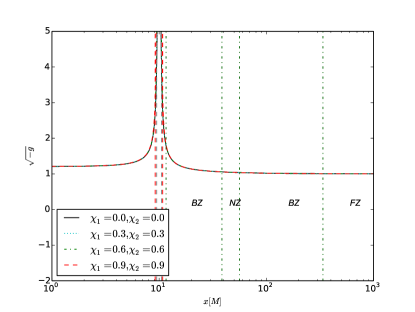
Figure 2: Comparison of the volume element, $\sqrt{-g}$, for the global metric for differing values of the spin parameter $\chi$, where both black holes have spin aligned with the orbital angular momentum of the binary.

III NUMERICAL ANALYSIS

To verify the correctness of the analytic metric approximating a spinning BHB spacetime, we developed a battery of different and independent tests to judge the quality of the analytic approximation as in Ref Mundim et al. (2014). We are mainly interested in identifying how much this analytic approximation deviates from the true solution to the Einstein’s equations. In order to achieve a reasonable, independent analysis of this approximation we resort then to the computation of spacetime scalar invariants and their comparison against their expected values for vacuum spacetimes. While these analysis might not be sufficient to judge all aspects of this new metric it is definitely necessary to assess its overall quality especially when compared against other analytic, approximative metrics.

We summarize in the following subsections which scalar invariants we have used in our analysis. We then present the results for this analytic metric. Discussion on how these scalar invariants are computed in our codes is left to the end of this section III.5.

III.1 Ricci Scalar

Using this global approximate metric, we calculate the Einstein tensor $G_{\mu\nu}$, the Ricci tensor $R_{\mu\nu}$, the Ricci Scalar $R$ and the relative Kretschmann invariant $K$ (see below) to test the validity of the approximate metric. If the BHB spacetime constructed is a valid vacuum solution, then it naturally must satisfy the ten Einstein equations in vacuum, $R_{\mu\nu}=0$. Therefore, any deviations from $R=g_{\mu\nu}R^{\mu\nu}=0$ can be interpreted as a measure of the violation to the Einstein equations that the global metric has incurred by the approximate construction. In the following analysis, we use the sign conventions laid out in Ref. Misner et al. (1973) (see also Wald’s “General Relativity” Wald (1984)) for all different geometric quantities entering the computation of Ricci scalar. Note also that we have used projections of the Ricci tensor along the hyperspace normal and into the time slices to compute the Hamiltonian and Momentum constraints, which are consistent with the Ricci scalar analysis we present.

III.2 Relative Kretschmann

In principle, it is possible to construct many invariants for the BHB problem. Here we present a new concept that we can use to evaluate the validity of the approximate, analytic metric. One of the pitfalls of using a quantity such as the Ricci scalar in analysis of the violation to the Einstein equations is that it is not a normalized quantity. The Ricci scalar can be large without bound, and it is therefore difficult to assign meaning to a numerical quantity in the Ricci scalar without a scale to compare our results with. The only scale that the Ricci scalar provides in vacuum is how far it deviates from zero. A Ricci scalar value of $10^{-9}$ is better than a value of $10^{-6}$, but that is all that we can really say about it. If we wish to use this as an assessment of the error, it becomes difficult to assign meaning to the results if they are far from zero.

It would therefore be desirable to have a quantity that both measured the violation of the Einstein equations and provides a scale, so values could be compared directly and we can easily interpret them.

For this purpose, we introduce an invariant that can still give us a measure of the violation to the Einstein equations and has the added benefit of being normalized: the relative Kretschmann curvature scalar.

We start with the definition of the Weyl tensor $C_{\mu\nu\rho\delta}$ from Ref. Wald (1978),

$$R_{\mu\nu\rho\delta}= C_{\mu\nu\rho\delta}+(g_{\mu[\rho}R_{\delta]\nu}-g_{\nu[\rho}R_{\delta]\mu})-\frac{1}{3}Rg_{\mu[\rho}g_{\delta]\nu}\,.$$ (61)

From here, we contract the Weyl tensor with itself, eventually yielding Kretschmann curvature scalar:

$$R_{\mu\nu\rho\delta}R^{\mu\nu\rho\delta}=C_{\mu\nu\rho\delta}C^{\mu\nu\rho\delta}+2R_{\mu\nu}R^{\mu\nu}-\frac{1}{3}R^{2}\,.$$ (62)

We now can say that if the solution is exact, we know that this contraction of the Riemann tensor should be equal exactly to the contraction of the Weyl tensor. In exact solutions to Einstein’s equations, contraction of the Riemann tensor and the Ricci scalar are both zero. Therefore, we can define a relative Kretschmann from the remainder:

$$K_{\rm rel}=\bigg{|}\frac{2R_{\mu\nu}R^{\mu\nu}-R^{2}/3}{R_{\mu\nu\rho\delta}R^{\mu\nu\rho\delta}}\bigg{|}\,,$$ (63)

which is the remainder from the exact vacuum solution normalized by the Kretschmann invariant $R_{\mu\nu\rho\delta}R^{\mu\nu\rho\delta}$. We expect that this value will be less than one anywhere in the global spacetime for small violations from the vacuum spacetime. For larger violations, it may be possible to have $K_{\rm rel}>1$. This is because there is no constraint for the energy-momentum tensor which is converted from the Ricci violation. We can now use this as a measure of the exactness of the solution, and plot the residual that we obtain to get an idea what the relative violation is to the true (exact) solution. Essentially this normalization introduces a scale to which we can compare the errors our approximation produces, giving us the desirable feature of having a direct way achieve this task in our spacetime.

III.3 Accuracy of the Global Metric: the Ricci Scalar

In Ref. Mundim et al. (2014), we showed how the violations of the Ricci scalar change as we increase the order of approximation for an equal mass non-spinning BHB spacetime. Fortunately as expected from the analytical point of view, those violations became smaller everywhere as we went from a first order metric (with the quadrupole (IZ)-1PN (NZ) matching) to a second order metric (with the octupole (IZ)-2PN (NZ) matching). We reproduce that result here in Fig. 3. Our work in this paper is the first step towards higher order of approximation for spinning BHBs. As shown in Sec. II.4, the matching for the spacetime construction is first order with the quadrupole order for the IZ and 1PN order for the NZ. Since we do not have at the moment a higher order spinning BHB spacetime to compare to, we use the first and second order metrics for non-spinning BHB as a reference for the spinning metric. The idea is make sure that the spinning BHB metric does not introduce any larger violations of the Ricci scalar than what we have already seen in the non-spinning case. As we can see in Fig. 3 this is fortunately the case. The first order matched spinning BHB metric results into Ricci violations that follow most closely the second order violations of the non-spinning metric for regions far away from the BHs and lies in between first and second order cases for regions closer to the BHs. The reason we obtain much better results for the first order spinning BHB metric than for the first order non-spinning BHB metric is that we are indeed using higher order spinning metric components here while keeping the matching to first order only. The rationale is that while we would like to have a consistent order counting in this work and a future one for second order one, we can already take advantage of higher order metric pieces with smaller Ricci violations right now for our upcoming gas and MHD simulations.

Figure 3: The absolute value of the Ricci scalar along the $x$ coordinate, at an initial separation of $20M$. We compare here the violations of the Ricci scalar for the spinning BHB metric against the non-spinning (NS) BHB first and second order metrics Mundim et al. (2014). It is interesting to note that the new spinning BHB metric has violations of the same order of magnitude as the previous non-spinning BHB metric. In this plot and the following plots, the horizon is denoted by the grey dashed vertical line, discussed in more detail in Fig. 5. The ISCO is the orange dashed vertical line (see Appendix C for details). The green dash-dotted vertical lines indicate the boundaries of the different zones, and are consistent for all of the subsequent plots. It is good to note here that the zone boundaries do change for differing spins, though not by much, so here we picked the fiducial zone boundary for the $\chi_{i}=0.9$ (highly spinning) and aligned case.

As we increase the spin parameter value, $\chi_{i}$, from its non-spinning value, $\chi_{i}=0$, to a very large spinning configuration, $\chi_{i}=0.9$, we observe very little variations in the Ricci violations in the NZ and FZ. That indicates the perturbation by spin addition to the system is small (see Fig. 4). As we zoom into the NZ, Fig. 5, the differences in violation amongst all spinning cases become more evident. Only at a small spacetime volume between the horizon location and a radius set by an ISCO for an individual BH do these violation differences span more than one order of magnitude. While of great importance to accurately describe the spacetime in the vicinity of a BH, it is not so crucial in determining particle or gas dynamics since they are expected to follow unstable circular orbits and accrete into the BH. We hope in a future work to improve on these violation differences between the spinning cases by introducing a second order asymptotic matching between the IZ and NZ.

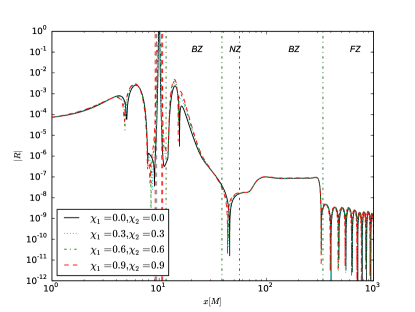
Figure 4: The absolute value of the Ricci scalar along $x$, at an initial separation of $20M$. The spin parameter is varied in this plot. We see that there is little qualitative variation in changing $\chi_{i}$.

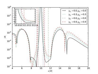
Figure 5: The absolute value of the Ricci scalar along $x$, for aligned spins, zoomed in on the inner region near the horizon. The horizon is denoted by the grey dashed vertical line, roughly at a position of $x_{h}=x_{\rm BH,1}\pm M/2$ on the $x$-axis, and is easier to distinguish here than in the previous plots. The ISCO is the orange dashed vertical line (see Appendix C for details). The inset shows the behavior close to the horizon.

Next we exploit the effects of spin anti-alignment with the orbital angular momentum. We fix our attention to the large spinning case, $|\chi_{i}|=0.9$. Again very little variation amongst the aligned, anti-aligned and the zero-sum cases is observed in the NZ and FZ (see Fig. 6). As we zoom into the IZ, Fig. 7, we can distinguish better among the cases, but none of them differ from each other more than two orders of magnitude at ISCO locus.

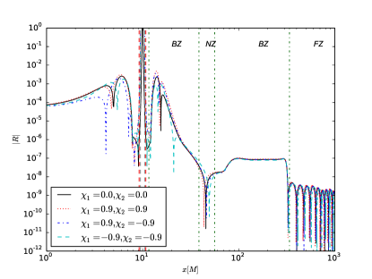
Figure 6: The absolute value of the Ricci scalar along $x$, at an initial separation of $20M$. This plot shows the spin parameter $\chi_{i}$ varied for anti-aligned spins.

Figure 7: The absolute value of the Ricci scalar along $x$, zoomed in near the BH to show the violation near the horizon. This plot shows the spin parameter $\chi_{i}$ varied for anti-aligned spins. The inset shows the behavior close to the horizon.

Finally we show snapshots of the Ricci scalar as the binary evolves in time, starting from a separation of $r_{12}=20M$ up until $r_{12}=8M$ roughly. We were careful to pick the instants of time when the BHs cross the x axis so that a comparison would be meaningful. As the separation decreases, the perturbation parameters become larger and larger leading to a poorer approximation of the spacetime. As expected then, the violations of the Ricci scalar increases with evolution time or decreasing binary separation as Fig. 8 shows for the aligned $\chi_{i}=0.9$ case. The take home lesson from that figure is that the violations do increase with time, but in a orderly and smooth fashion.

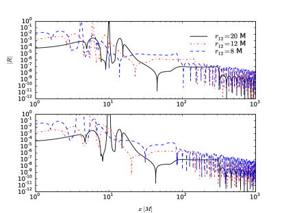
Figure 8: The absolute value of the Ricci scalar along $x$, at an initial separation of $20M$, $12M$, and $8M$, for spins $\chi_{1}=\chi_{2}=0.0$ (top) and $\chi_{1}=\chi_{2}=0.9$ aligned (bottom). Note that the violation increases smoothly as we decrease in orbital separation. This gives good indication that the dynamics is not introducing any spurious error into the metric.

III.4 Accuracy of the Global Metric: the Relative Kretschmann

Here we plot the accuracy of the metric with respect to the relative Kretschmann invariant, to contrast the Ricci analysis above.

As we can see from Fig. 9, the Kretschmann invariant becomes large near the BHs, and falls off as $1/r^{6}$ as we move away from the BHs. This means that any error in the FZ will be divided by a very small number, and so the relative Kretschmann will be large in the FZ. Therefore, in the weak gravitational field, the relative Kretschmann cannot be used to meaningfully measure the accuracy. On the other hand, it will be extremely small in the IZ where it is being divided by a very big number. Thus, when the true gravitational field is strong, the relative Kretschmann can be used as a meaningful measure of the spacetime accuracy.

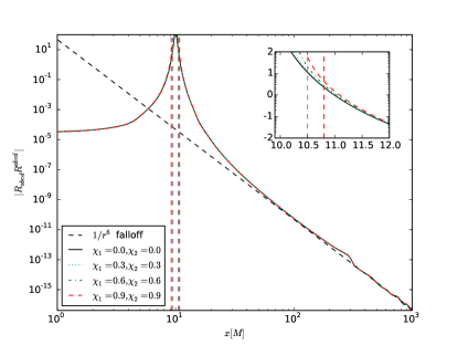
Figure 9: The Kretschmann invariant calculated for the BHB spacetime for differing values of spin, all of which are aligned with the orbital angular momentum of the binary, at an initial separation of $r_{12}=20M$. The $1/r^{6}$ behavior seen far from the two BHs ($\sim 40M$) is consistent with the value of the Kretschmann in the single Schwarzschild BH case: $K=48M^{2}/r^{6}$, where $M$ is the total mass of the binary centered on the origin. The inset shows the behavior close to the horizon, where the spin effects become noticeable. The Kretschmann becomes large as it approaches a BH, because the invariant blows up at a true singularity.

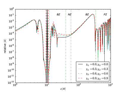
Figure 10: The relative Kretschmann for an initial separation of $r_{12}=20M$, with a grid resolution of $0.0125$. In this plot, we are plotting aligned spinning BHs, and increasing the dimensionless spin parameter $\chi_{i}$ from non spinning to highly spinning. Observe the normalized behavior that these plots exhibit. The violation to this invariant is very good close to the horizon due to the way that we are normalizing. See Fig. 9 for the normalization function.

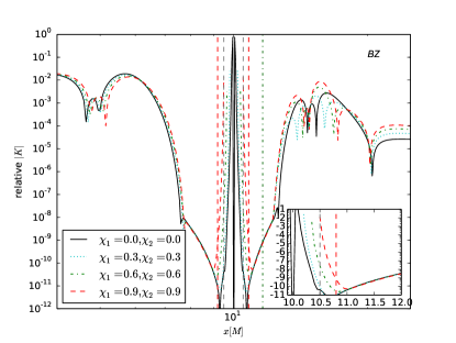
Figure 11: Zoomed in view of Fig. 10 around the IZ. The inset shows the behavior close to the horizon.

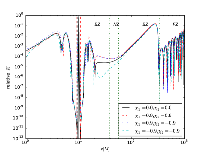
Figure 12: The relative Kretschmann for an initial separation of $r_{12}=20M$, with a grid resolution of $0.0125$ for varying values of the dimensionless spin parameter $\chi_{i}$. In this plot, we are looking at what the relative Kretschmann does for anti-aligned BHs with high $\chi_{i}$ values. Observe the normalized behavior that these plots exhibit. The violation to this invariant is very good close to the horizon, due to the way that we are normalizing. See Fig. 9 for the normalization function.

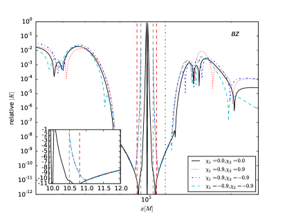
Figure 13: Zoomed in view of Fig. 12 around the IZ. The inset shows the behavior close to the horizon.

We briefly discuss the FZ behavior in Figs. 10 and 12. In the FZ, the solution does not follow the $1/r$ behavior that is expected. This is because the coefficients are calculated in the PN approximation. We can show this schematically as follows. Imagine a schematic expression of the FZ metric,

$$h_{\mu\nu}^{\rm FZ}\sim\frac{H_{\mu\nu}}{r}\exp(-i\omega(t-r))+O(1/r^{2})\,,$$ (64)

where $H_{\mu\nu}$ is evaluated from the PN multipole sources. When we plot the Ricci scalar in the FZ, we have a $1/r$ factor that will act as a damping term. However, in the relative Kretschmann calculation, this $1/r$ dependence cancels out due to the $r$ dependence in the Kretschmann invariant. Therefore, any error accumulated in the PN expression for $H_{\mu\nu}$ will become an important contribution to the overall error in the FZ, leading to some large finite amplitude of the Kretschmann at large $r$.

The Kretschmann invariant is not an independent measure of the error in the approximations, just another way to look at the violation of the spacetime. The Ricci scalar contains information about the spacetime violation, and since the behavior of the Ricci scalar in the FZ is damped as expected, the observed behavior in the relative Kretschmann is not necessarily a concern given the issues with this diagnostic discussed earlier due to the finite PN expression being divided by a small value of the Kretschmann. This is by no means a proof that the error in the FZ is not dominated by noise that could be suppressed by taking the code to a higher precision, however, because the Ricci scalar shows good behavior in the FZ, it is not worth the analysis that would be required since other complementary invariants have shown excellent small violations in the FZ.

For these reasons, although the relative Kretschmann is a good way to measure errors in the IZ, where the fields are strong and dynamical, it is a poor way to measure the overall accuracy of the global metric in the weak field limit far from the compact sources.

III.5 Numerical methods

In order to compute the several geometric quantities needed for our analysis partial derivatives of the metric components are needed. One could try to obtain these derivatives analytically, in a closed form, for each piece of the metric used when composing the global metric, however this would result into extremely large expressions which could potentially defeat the goal of obtaining analytic approximations of BHB spacetimes that are cheaper to compute than a full general relativistic numerical computation. In addition this fully analytic approach to the computation of the derivatives would be extremely tricky to implement in the BZs where not only we need to worry about the metric matching but also the matching of its derivatives. These analytic complications give us incentive to compute these derivatives numerically. In all computations showed in this paper we have discretized the partial derivatives using a centered, fourth order finite difference stencil. In Fig. 14 we show the Ricci scalar convergence factor ($Q(t=0,x)=(R^{4h}-R^{2h})/(R^{2h}-R^{h})=2^{p}+O(h)$, where $h$ is the mesh spacing and $p=4$ in our case. See Ref. Mundim et al. (2014) for more details) for several different resolutions demonstrating convergence to the continuum solution to the $4th$ order of approximation. Since the solution spans several scales of length, different requirements in terms of mesh spacings is needed to resolve the solution. For example, on the top panel the highest resolutions used to compute the convergence factor, $h_{H}/M=\{0.025,\,0.0125,\,0.00625\}$, does resolve well the solution features in the vicinity of the BH location, $x_{{\rm BH},1}/M=10$ in this case. In addition we can see clearly the convergence factor tending to $16.0$ around $x/M=9$ or $x/M=11$ as we increase the resolution used in $Q_{L}$ to the ones in $Q_{M}$ and $Q_{H}$, a clear indication of $4th$ order convergence. However it is interesting to note that the high resolution mesh spacing set drives the convergence factor outside the convergence regime approximately outside the interval $[7M,\,13M]$. This is mainly due to the limited precision to represent numbers in these computations (double precision in our case). Subtractions of very similar numbers results in catastrophic loss of precision which in turn results in poor convergence order computation. A quadruple precision version of the code was used in the past to evaluate and confirm this loss of precision, however its general use for our current simulations is prohibitively expensive and we do not report its results here.

One interesting reading from Fig. 14 concerns identifying the mesh spacing requirement for each of the zones describing our metric. For example, in the vicinity of the BH location, $[10.5M,\,11.5M]$ we can safely say that the set of mesh spacings $h/M=\{0.00625,\,0.0125,\,0.025,\,0.05\}$ lies within the convergence radius of the $4th$ order scheme. As this $x$ interval extends beyond, roughly $[11.5M,\,20.0M]$, the requirement changes to the set of $h/M=\{0.0125,\,0.025,\,0.05,\,0.1\}$. As we increase the interval farther away, $[20.0M,\,50.0M]$, the set of $h/M=\{0.1,\,0.2,\,0.4,\,0.8\}$ seem reasonable. As we go farther away the BH location the resolution, $[50M,\,200M]$, the resolution requirement drops for $h=\{0.8,\,1.6,\,3.2,\,6.4\}$ approximately. Finally as we extend to intervals of $[200M,\,1000M]$ and beyond, mesh spacings of $h/M=\{3.2,\,6.4,\,12.8,\,25.6\}$ seem reasonable to obtain converging solutions. From these studies it is clear then that we are able to obtain $4th$ order converging solutions from the IZ to the FZ if we are careful in selecting the appropriate mesh spacings.

Figure 14: Convergence factor along $x$. Each of the above panels show the Ricci scalar convergence factor $Q$ at $t=0$ along the coordinate $x$-axis for different intervals in $x$, depending on the set of mesh spacing used in the convergence factor computation. On all panels the red dotted line represents the convergence factor for the low resolution mesh spacing set used in that panel, while the blue dashed and black solid lines the medium and high resolution mesh spacing set, respectively. The green horizontal dashed line at $Q=16.0$ is the theoretical solution at infinite resolution $h=0$. On the top panel, the low resolution mesh set, $h_{L}/M=\{0.1,\,0.05,\,0.025\}$, is used to compute $Q_{L}$, while the medium and high resolution ones are $h_{M}/M=\{0.05,\,0.025,\,0.0125\}$ and $h_{H}/M=\{0.025,\,0.0125,\,0.00625\}$, respectively. We masked out $Q_{H}$ outside the interval $[7M,\,13M]$ to avoid noise due to round-off precision errors. On the second panel from above, the low resolution set is $h_{L}/M=\{0.8,\,0.4,\,0.2\}$, while the medium and high ones are $h_{M}/M=\{0.4,\,0.2,\,0.1\}$ and $h_{H}/M=\{0.2,\,0.1,\,0.05\}$, respectively. We also mask out $Q_{H}$ and $Q_{M}$ for $x>25M$ and $x>35M$, respectively, to avoid round-off noise. On the third panel, we use $h_{L}/M=\{6.4,\,3.2,\,1.6\}$, $h_{M}/M=\{3.2,\,1.6,\,0.8\}$ and $h_{L}/M=\{1.6,\,0.8,\,0.4\}$. We mask out $Q_{H}$ and $Q_{M}$ for $x>90M$ and $x>140M$, respectively. Finally on the bottom panel, we use $h_{L}/M=\{51.2,\,25.6,\,12.8\}$, $h_{M}/M=\{25.6,\,12.8,\,6.4\}$ and $h_{L}/M=\{12.8,\,6.4,\,3.2\}$. These different sets of resolutions were used here to emphasize the mesh spacings required to be in the convergence regime for different zones.

III.6 Orbital hang-up effect, and long time evolutions of the BHB

In Ref. Gallouin et al. (2012) the Ricci violation was shown for an initial spatial hypersurface. This work has presented figures for the Ricci violation and relative Kretschmann by using Eq. (52) as the coordinate transformation for long time evolutions of our dynamic spacetime, these figures just capture a snapshot at an instant in time which is basically the same procedure that was used for the initial data. This means that we just need the EOM at an instant in time, and it is not necessary to solve the EOM. Therefore, it is not clear that we have introduced an appropriate EOM for long time evolutions of the BHB system, and thus to confirm our results we present the orbital evolutions.

A natural way to test this implementation of the EOM is to see if this work can reproduce any of the known effects of spin dynamics in aligned non-precessing systems, such as the orbital hang-up effect discovered in Ref. Campanelli et al. (2006b). Recovering the hang up effect is an easy way to show the correctness in the implementation of the EOM for the binary. The orbital hang-up effect is an effect where the spin of the individual BHs add to the orbital angular momentum of the binary, causing the orbit to inspiral more slowly, as it has to dissipate more angular momentum. This leads to a pile up of the orbits, causing the “hang-up”. For the following plot, we will be considering equal mass BHs in quasi circular orbits, with dimensions in terms of the total mass $M=m_{1}+m_{2}$ of the binary. This effect was shown to be the strongest at merger in Ref. Campanelli et al. (2006b), but as we show here it also has an effect in the PN regime.

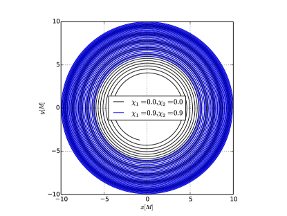
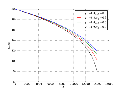
Figure 15: The top panel is the orbital hang-up effect shown by plotting the individual trajectories of BH1. Note that the orbits get bunched up as the spin is increased from $\chi_{1}=\chi_{2}=0.0$ to $0.9$. Both of the BH spins are aligned with the orbital angular momentum of the binary. The bottom panel shows the orbital hang-up effect as a decrease in the orbital separation as a function of time for varying aligned spin parameters, with the fiducial spin values chosen to coincide with the spins used in the Ricci and relative Kretschmann analyzes. For both the top and bottom panels, the evolution was terminated at $14000M$ in time.

This effect can be seen clearly in Fig. 15. Had the spins been anti-aligned, the reverse would be seen, with the highly spinning BHs plunging quickly compared to the non spinning case. Comparisons to the orbital dynamics in Refs. Noble et al. (2012) and Scheel et al. (2015) yield good confirmation between the trajectory plotted and the non spinning trajectory here, offering reassurance that the correct dynamics are being calculated in the PN approximation, and thus that our results are valid for long time evolutions.

IV DISCUSSION

We have constructed a globally analytic, approximate BHB spacetime via asymptotically matching BH perturbation theory to PN formalism farther out to a PM spacetime even further away. The procedure of asymptotic matching had to be generalized from Ref. Gallouin et al. (2012) to be valid on all spatial hypersurfaces, instead of a small group of initial hypersurfaces near $t-t_{0}$. Matching the metrics in this way allows us to construct a global metric, which is correct until the PN approximation breaks down, around $10M$ in orbital separation.

The validity of this global metric was extensively tested using several different techniques. We first calculated the absolute value of the Ricci scalar and plotted it along a particular axis and compared it with the exact solution value $R=0$. Then the evolution of the Ricci scalar was explored, to ensure that there were no sporadic errors in the evolution that would contribute unduly to the overall error. Fortunately, the behavior observed in this evolution was a smooth increase in the violation to the Einstein field equations due to the slow motion assumption breaking down as the BHs inspiral.

To contrast with the Ricci scalar analysis, we performed an analysis by using the relative Kretschmann $K_{\rm rel}$ in Eq. (63). However, it was noticed that this measure of the error in the global metric is not the best in the FZ, since the FZ behavior is not damped, and indeed appears to be the largest contributor of error. As a result of this analysis, though the relative Kretschmann has the attractive feature of being an invariant with a natural scale of comparison, we will be using the Ricci scalar as the measure of the accuracy of the global metric out to the FZ, electing to use the Kretschmann for studies of the violation close to either BH.

This metric is valid dynamically and for long time evolutions, which makes it an ideal metric to use when studying effects happening in the relativistic regime of BHBs. The immediate application of this metric is to implement it into the Harm3d code, which can then be used to study MHD in the context of the BHB problem with spins. This will allow new studies of accretion physics, giving us the theoretical tools to make predictions for the EM signatures of BHBs with spin.

Certain practical considerations are required when talking about this global metric construction. In this paper, we have considered only one choice of transition function, which is summarized in Appendix A. The transition functions’ arguments were chosen by pragmatic considerations; experimentally shown to give a lower violation to the Einstein field equations, and not necessarily by any mathematical arguments, such as the Frankenstein theorems of Ref. Yunes (2007).

A study which will be important for the future is an in depth analysis of the transition region near the IZ-NZ BZ. From preliminary hydrodynamic simulations, the mini disks around the individual BHs fall entirely in the BZ, and the choice of transition function may have a significant impact on the spacetime, and thus the gas dynamics will be impacted. Practical choices of the free parameters need to be explored further and will be highly valued for upcoming MHD runs.

Another test that can be done is to explore test particle trajectories in the spacetime. This powerful tool will give us a good idea of how the spacetime is doing complementary to the violation of the Ricci scalar and relative Kretschmann invariant. This is being developed currently, and will be explored in detail in a future paper.

A final step for this project is to generalize this to arbitrarily aligned spins, which will lead to precession. This has the added benefit of being able to study even more interesting spin effects such as transitional precession and spin flips. This will require refinement in our techniques. The IZ metric will have to take into account that the tidal fields are no longer solely along the $r$ direction, but shifted so that the spin axis is arbitrarily aligned with the orbital angular momentum. The EOM need to be updated to take into account the higher order spin dynamics, and the metric will need to be modified to generate spins along any direction. Though this process will be arduous, a fully analytic spacetime describing a precessing, arbitrarily aligned, spinning BHB spacetime will allow for GRMHD simulations to explore completely new territory of gas dynamics in the context of precessing BH spins.

Appendix A Transition functions

When constructing the global metric, we must introduce appropriate transition functions in the BZs to avoid erroneous behaviors Yunes (2007). In this analysis, we follow Ref. Mundim et al. (2014), and use the following transition function:

$$f(r,\,r_{0},\,w,\,q,\,s)=\left\{\begin{array}[]{lr}0\,,&r\leq r_{0}\,,\\ \displaystyle{\frac{1}{2}}\left\{1+\tanh\left[\frac{s}{\pi}\left(\chi(r,\,r_{0},\,w)-\frac{q^{2}}{\chi(r,\,r_{0},\,w)}\right)\right]\right\}\,,&\hskip 25.60747ptr_{0}<r<r_{0}+w\,,\\ 1\,,&r\geq r_{0}+w\,,\end{array}\right.$$ (68)

where $\chi(r,r_{0},w)=\tan[\pi(r-r_{0})/(2w)]$, and $r_{0}$, $w$, $q$ and $s$ are parameters. Great detail on this transition function can be found in Refs. Johnson-McDaniel et al. (2009); Yunes et al. (2006); Yunes and Tichy (2006). This transition function uses different parameters in each of the BZs, that are modified from Ref. Johnson-McDaniel et al. (2009).

In the analysis, we started by using the parameters from Ref. Mundim et al. (2014):

$$f_{\rm near}=f(x,\,2.2m_{2}-m_{1}r_{12}/M,\,r_{12}-2.2M,\,1,\,1.4),$$ (69)

$$f_{\rm inner,\,A}=f(r_{A},\,0.256r^{T}_{A},\,3.17(M^{2}r^{5}_{12})^{1/7},\,0.2,\,r_{12}/M).$$ (70)

Here $r^{T}_{A}$ is the transition function radius, derived by requiring the uncontrolled remainders of the IZ and NZ approximations be roughly equal. The NZ-FZ transition function is unchanged with respect to Ref. Mundim et al. (2014), and the details of this choice of transition function can be explored in that paper. It should be noted that although we should formally use the transition functions given in Ref. Gallouin et al. (2012) due to the matching order according to the Frankenstein theorems of Ref. Yunes (2007), we have used the above transition functions because it was found by experiment that they give overall better results in the Ricci calculation. While this is not mathematically rigorous, it is a practical choice that we made to minimize the violation to the Einstein field equations represented by the Ricci scalar and the relative Kretschmann invariant.

It is also noted here that in practice we use the value $s=b/M$ where $b$ is a (constant) initial orbital separation, as opposed to $r_{12}/M$ which is time dependent. This choice was made in Ref. Mundim et al. (2014), so to compare as directly as possible, we use the same $s$ parameter as is used there.

In the course of doing large separation runs ($\approx 100M$) with the non spinning global metric, a problem was found with the IZ-NZ transition function. At large separation, the value of $s=r_{12}/M$ becomes large. As discussed in Ref. Yunes and Tichy (2006), $q$ determines the location where the transition function equals $1/2$, and $s$ sets the slope, given by $s(1+q^{2})/(2w)$. When we discuss the Ricci scalar of the spacetime, $s$ becomes more sensitive than $q$ in setting the slope for fixed $r_{0}$ and $w$. Due to the value of $r_{12}$ setting the slope, in large separation runs with $m_{1}=m_{2}=m/2$, the second derivative of the transition function $f_{\rm inner,\,A}$ can become very large. Because of this, a new value of $s$ is suggested to minimize the absolute value of the second derivative of this transition function. Due to analytic testing of the transition function, this $s$ parameter was set to $12$ for our future work and implementation into Harm3d.

Of course, there are many other parameters that set the transition function, all of which can have wildly different values. In future work, it would be nice to have a way of optimizing the parameters to give the minimum violation to the Ricci scalar. This could be achieved by using a Monte Carlo simulation to explore this parameter space and pinpoint the ideal values of the different parameters, while still being a valid transition function (i.e. obeying the Frankenstein theorems Yunes (2007)). This will be reserved for future work.

Appendix B Ingoing Kerr Coordinates to Cook-Scheel Harmonic Coordinates

The NZ metric is calculated in the PN harmonic coordinates, but to accurately describe gas dynamics close to the event horizons, it is desirable to have the horizon penetrating property. Therefore, the Cook-Scheel harmonic (CS-H) coordinates Cook and Scheel (1997) are ideal for the Kerr spacetime, which describes the background IZ metric.

Here we change the notation used throughout the paper slightly because this coordinate transformation is for a single BH. Therefore, in this appendix only, we will take $M$ to be the mass of the individual Kerr BH, and not the total mass.

The IZ metric presented in Ref. Yunes and González (2006), however, is in the ingoing Kerr (IK) coordinates. Noting the similarities between the more familiar Boyer-Lindquist (BL) coordinates, $r_{\rm IK}=r_{\rm BL}$ and $\theta_{\rm IK}=\theta_{\rm BL}$, we can rewrite the coordinate transformation from the IK ($v_{\rm IK},\,r_{\rm IK},\,\theta_{\rm IK},\phi_{\rm IK}$) coordinates to CS-H ($t_{\rm H},\,x_{\rm H},\,y_{\rm H},\,z_{\rm H}$) coordinates :

$$t_{\rm H} =v_{\rm IK}-r_{\rm IK}+2\,M\,\ln\left|\frac{2\,M}{r_{\rm IK}-r_{-}}\right|\,,$$

$$x_{\rm H}+i\,y_{\rm H} =(r_{\rm IK}-M+i\,a)e^{i\,\phi_{\rm IK}}\,\sin\theta_{\rm IK}\,,$$

$$z_{\rm H} =(r_{\rm IK}-M)\cos\theta_{\rm IK}\,.$$ (71)

It is noted that the following calculations are similar to to the summary in the appendix of Ref. Yunes and González (2006) for the coordinate transformation between the IK and Kerr-Schild coordinates. To calculate the Jacobian to transform tensors, we rewrite the above relations as

$$x_{\rm H} =\left[(r_{\rm IK}-M)\,\cos\phi_{\rm IK}-a\,\sin\phi_{\rm IK}\right]\sin\theta_{\rm IK}\,,$$

$$y_{\rm H} =\left[(r_{\rm IK}-M)\,\sin\phi_{\rm IK}+a\,\cos\phi_{\rm IK}\right]\sin\theta_{\rm IK}\,,$$

$$z_{\rm H} =(r_{\rm IK}-M)\cos\theta_{\rm IK}\,.$$ (72)

Here, we calculate the radial coordinate in the CS-H as

$$r_{\rm H}^{2} =x_{\rm H}^{2}+y_{\rm H}^{2}+z_{\rm H}^{2}$$ (73)

$$=r_{\rm IK}^{2}-2Mr_{\rm IK}+M^{2}+a^{2}-a^{2}\cos^{2}\theta_{\rm IK}\,.$$ (74)

When we solve the above equation with respect to $r_{\rm IK}$, there are four solutions, and one of the solutions,

$$r_{\rm IK}= \frac{1}{2}\biggl{[}2\sqrt{r_{\rm H}^{4}-2a^{2}r_{\rm H}^{2}+a^{4}+4a^{2}z_{\rm H}^{2}}$$ (75)

$$+2r_{\rm H}^{2}-2a^{2}\biggr{]}^{1/2}+M\,,$$ (76)

gives the appropriate radial coordinate for large $r_{\rm H}$. Therefore, the inverse transformation is summarized as

$$r_{\rm IK} =\sqrt{\frac{r_{\rm H}^{2}-a^{2}+W}{2}}+M\,,$$

$$\theta_{\rm IK} =\arccos\frac{z_{\rm H}}{(r_{\rm IK}-M)}\,,$$

$$\phi_{\rm IK} =\arctan{\frac{(r_{\rm IK}-M)\,y_{\rm H}-a\,x_{\rm H}}{(r_{\rm IK}-M)\,x_{\rm H}+a\,y_{\rm H}}}\,,$$ (77)

and

$$v_{\rm IK} =t_{\rm H}+r_{\rm IK}-2\,M\,\ln\left|\frac{2\,M}{r_{\rm IK}-r_{-}}\right|\,,$$ (78)

where

$$W =\sqrt{(r_{\rm H}^{2}-a^{2})^{2}+4\,a^{2}\,z_{\rm H}^{2}}\,.$$ (79)

We have the useful relations,

$$\sin\theta_{\rm IK} =\sqrt{\frac{x_{\rm H}^{2}+y_{\rm H}^{2}}{(r_{\rm IK}-M)^{2}+a^{2}}}\,,$$

$$\sin\phi_{\rm IK} =\frac{(r_{\rm IK}-M)\,y_{\rm H}-a\,x_{\rm H}}{[((r_{\rm IK}-M)^{2}+a^{2})(x_{\rm H}^{2}+y_{\rm H}^{2})]^{1/2}}\,,$$

$$\cos\phi_{\rm IK} =\frac{(r_{\rm IK}-M)\,x_{\rm H}+a\,y_{\rm H}}{[((r_{\rm IK}-M)^{2}+a^{2})(x_{\rm H}^{2}+y_{\rm H}^{2})]^{1/2}}\,.$$ (80)

Using the above inverse transformation, the Jacobian for this coordinate transformation, $\partial x^{a}_{\rm IK}/\partial x^{b}_{\rm H}$ is calculated as

$$\frac{\partial v_{\rm IK}}{\partial t_{\rm H}}= 1\,,$$

$$\frac{\partial v_{\rm IK}}{\partial x_{\rm H}}= \frac{x_{\rm H}}{2\,(r_{\rm IK}-M)}\left(1+\frac{r_{\rm H}^{2}-a^{2}}{W}\right)\left(1+\frac{2\,M}{r_{\rm IK}-r_{-}}\right)\,,$$

$$\frac{\partial v_{\rm IK}}{\partial y_{\rm H}}= \frac{y_{\rm H}}{2\,(r_{\rm IK}-M)}\left(1+\frac{r_{\rm H}^{2}-a^{2}}{W}\right)\left(1+\frac{2\,M}{r_{\rm IK}-r_{-}}\right)\,,$$

$$\frac{\partial v_{\rm IK}}{\partial z_{\rm H}}= \frac{z_{\rm H}}{2\,(r_{\rm IK}-M)}\left(1+\frac{r_{\rm H}^{2}+a^{2}}{W}\right)\left(1+\frac{2\,M}{r_{\rm IK}-r_{-}}\right)\,,$$

$$\frac{\partial r_{\rm IK}}{\partial t_{\rm H}}= 0\,,$$

$$\frac{\partial r_{\rm IK}}{\partial x_{\rm H}}= \frac{x_{\rm H}}{2\,(r_{\rm IK}-M)}\left(1+\frac{r_{\rm H}^{2}-a^{2}}{W}\right)\,,$$

$$\frac{\partial r_{\rm IK}}{\partial y_{\rm H}}= \frac{y_{\rm H}}{2\,(r_{\rm IK}-M)}\left(1+\frac{r_{\rm H}^{2}-a^{2}}{W}\right)\,,$$

$$\frac{\partial r_{\rm IK}}{\partial z_{\rm H}}= \frac{z_{\rm H}}{2\,(r_{\rm IK}-M)}\left(1+\frac{r_{\rm H}^{2}+a^{2}}{W}\right)\,,$$

$$\frac{\partial\theta_{\rm IK}}{\partial t_{\rm H}}= 0\,,$$

$$\frac{\partial\theta_{\rm IK}}{\partial x_{\rm H}}= \frac{x_{\rm H}\,z_{\rm H}}{2\,(r_{\rm IK}-M)^{2}}\left(1+\frac{r_{\rm H}^{2}-a^{2}}{W}\right)$$ (81)

$$\times\left((r_{\rm IK}-M)^{2}-z_{\rm H}^{2}\right)^{-1/2}\,,$$

$$\frac{\partial\theta_{\rm IK}}{\partial y_{\rm H}}= \frac{y_{\rm H}\,z_{\rm H}}{2\,(r_{\rm IK}-M)^{2}}\left(1+\frac{r_{\rm H}^{2}-a^{2}}{W}\right)$$ (82)

$$\times\left((r_{\rm IK}-M)^{2}-z_{\rm H}^{2}\right)^{-1/2}\,,$$

$$\frac{\partial\theta_{\rm IK}}{\partial z_{\rm H}}= -\left[1-\frac{z_{\rm H}^{2}}{2\,(r_{\rm IK}-M)^{2}}\left(1+\frac{r_{\rm H}^{2}+a^{2}}{W}\right)\right]$$ (83)

$$\times\left((r_{\rm IK}-M)^{2}-z_{\rm H}^{2}\right)^{-1/2}\,,$$

$$\frac{\partial\phi_{\rm IK}}{\partial t_{\rm H}}= 0\,,$$

$$\frac{\partial\phi_{\rm IK}}{\partial x_{\rm H}}= -\frac{y_{\rm H}}{x_{\rm H}^{2}+y_{\rm H}^{2}}+\frac{a\,x_{\rm H}}{2\,(r_{\rm IK}-M)((r_{\rm IK}-M)^{2}+a^{2})}$$ (84)

$$\times\left(1+\frac{r_{\rm H}^{2}-a^{2}}{W}\right)\,,$$

$$\frac{\partial\phi_{\rm IK}}{\partial y_{\rm H}}= \frac{x_{\rm H}}{x_{\rm H}^{2}+y_{\rm H}^{2}}+\frac{a\,y_{\rm H}}{2\,(r_{\rm IK}-M)((r_{\rm IK}-M)^{2}+a^{2})}$$ (85)

$$\times\left(1+\frac{r_{\rm H}^{2}-a^{2}}{W}\right)\,,$$ (86)

$$\frac{\partial\phi_{\rm IK}}{\partial z_{\rm H}}= \frac{a\,z_{\rm H}}{2\,(r_{\rm IK}-M)((r_{\rm IK}-M)^{2}+a^{2})}$$ (87)

$$\times\left(1+\frac{r_{\rm H}^{2}+a^{2}}{W}\right)\,.$$ (88)

The right hand side of the above equations includes the IK and CS-H coordinates because the expressions give a compact form. Although there is a apparent divergent behavior at $r_{\rm IK}=M$, this can be removed by using

$$r_{\rm IK}-M= \sqrt{\frac{r_{\rm H}^{2}-a^{2}+W}{2}}\,.$$ (89)

Finally, the perturbed metric in the IK coordinates is transformed to the CS-H coordinates as

$$g_{\mu\nu}^{\rm H}=\frac{\partial x^{\mu^{\prime}}_{\rm IK}}{\partial x^{\mu}_{\rm H}}\frac{\partial x^{\nu^{\prime}}_{\rm IK}}{\partial x^{\nu}_{\rm H}}g_{\mu^{\prime}\nu^{\prime}}^{\rm IK}\,.$$ (90)

This IZ metric in the CS-H coordinates will then be matched to the NZ metric.

Appendix C Details about the horizon and the innermost stable circular orbit

In our analysis of the validity of the spacetime, it is helpful to understand the location of the BH horizon and the ISCO in the PNH coordinates. We discuss the coordinate transformation from the BL to the CS-H coordinates again, because various useful results have been derived in the BL coordinates.

The coordinate transformation from the BL coordinates ($t_{\rm BL},\,r_{\rm BL},\,\theta_{\rm BL},\,\phi_{\rm BL}$) to the CS-H coordinates ($t_{\rm H},\,x_{\rm H},\,y_{\rm H},\,z_{\rm H}$) is given by

$$t_{\rm H} =t_{\rm BL}+\frac{r_{+}^{2}+a^{2}}{r_{+}-r_{-}}\,\ln\left|\frac{r_{\rm BL}-r_{+}}{r_{\rm BL}-r_{-}}\right|\,,$$

$$x_{\rm H}+i\,y_{\rm H} =(r_{\rm BL}-M+i\,a)e^{i\,\varphi}\,\sin\theta_{\rm BL}\,,$$

$$\qquad\varphi =\phi_{\rm BL}+\frac{a}{r_{+}-r_{-}}\,\ln\left|\frac{r_{\rm BL}-r_{+}}{r_{\rm BL}-r_{-}}\right|\,,$$

$$z_{\rm H} =(r_{\rm BL}-M)\cos\theta_{\rm BL}\,,$$ (91)

where $r_{\pm}=M\pm\sqrt{M^{2}-a^{2}}$ denote the event horizon ($r_{+}$) and Cauchy horizon ($r_{-}$) in the BL coordinates, and $\varphi$ is same as $\phi_{\rm IK}$ in Appendix B.

The following equations are useful to understand the CS-H coordinates.

$$x_{\rm H}^{2}+y_{\rm H}^{2} =[(r_{\rm BL}-M)^{2}+a^{2}]\,\sin^{2}\theta_{\rm BL}$$ (92)

$$=[(r_{\rm BL}-M)^{2}+a^{2}]\left(1-\frac{z_{\rm H}^{2}}{(r_{\rm BL}-M)^{2}}\right)\,,$$ (93)

$$r_{\rm H}^{2} =(r_{\rm BL}-M)^{2}+a^{2}\,\sin^{2}\theta_{\rm BL}\,,$$ (94)

$$r_{\rm H}\,\cos\theta_{\rm H} =z_{\rm H}=(r_{\rm BL}-M)\cos\theta_{\rm BL}\,,$$ (95)

$$\phi_{\rm H} =\arctan\frac{y_{\rm H}}{x_{\rm H}}=\phi_{\rm a}+\varphi\,;$$ (96)

$$\phi_{\rm a} =\arctan\frac{a}{r_{\rm BL}-M}\,.$$ (97)

The event horizon ($r_{\rm BL}=r_{+}$) is located at $r_{\rm H}=\sqrt{M^{2}-a^{2}\cos^{2}\theta_{\rm BL}}$ in the CS-H coordinates from the transformations above. We also will use this location in the PNH coordinates as a rough estimation of the event horizon because the transformation from the CS-H to the PNH coordinates is treated perturbatively, so the location of the horizon will not change much. On the equatorial plane ($\theta_{\rm BL}=\theta_{\rm H}=\pi/2$), we have the event horizon at

$$r_{\rm H}=M\,,$$ (98)

which is independent of the spin parameter, $a$. It is noted that there is a coordinate singularity at $r_{\rm BL}=M$, i.e., $r_{\rm H}=|a|\sin\theta_{\rm BL}$ ($x_{\rm H}^{2}+y_{\rm H}^{2}\leq a^{2}$) and $z_{\rm H}=0$ Cook and Scheel (1997).

The inverse transformation is obtained as

$$r_{\rm BL}= \frac{1}{\sqrt{2}}[r_{\rm H}^{2}-a^{2}+((r_{\rm H}^{2}-a^{2})^{2}+4\,a^{2}\,z_{\rm H}^{2})^{1/2}]^{1/2}+M$$ (99)

$$= R_{\rm H}+M\,,$$ (100)

$$t_{\rm BL}= t_{\rm H}-\frac{(M+\sqrt{M^{2}-a^{2}})^{2}+a^{2}}{2\,\sqrt{M^{2}-a^{2}}}$$ (101)

$$\times\ln\left|\frac{R_{\rm H}-\sqrt{M^{2}-a^{2}}}{R_{\rm H}+\sqrt{M^{2}-a^{2}}}\right|\,,$$ (102)

$$\theta_{\rm BL}= \arccos\frac{z_{\rm H}}{r_{\rm BL}-M}=\arccos\frac{z_{\rm H}}{R_{\rm H}}\,,$$ (103)

$$\phi_{\rm BL}= \phi_{\rm H}-\phi_{\rm a}-\frac{a}{r_{+}-r_{-}}\,\ln\left|\frac{r_{\rm BL}-r_{+}}{r_{\rm BL}-r_{-}}\right|$$ (104)

$$= \arctan\frac{y_{\rm H}}{x_{\rm H}}-\arctan\frac{a}{R_{\rm H}}$$ (105)

$$-\frac{a}{2\,\sqrt{M^{2}-a^{2}}}\,\ln\left|\frac{R_{\rm H}-\sqrt{M^{2}-a^{2}}}{R_{\rm H}+\sqrt{M^{2}-a^{2}}}\right|\,.$$ (106)

Note here that $r_{\rm H}$ and $R_{\rm H}$ are different. The Taylor expansion with respect to small $a$ and $M$ of the above relation gives the same equations as in Ref. Hergt and Schaefer (2008). But in Ref. Hergt and Schaefer (2008), we find the time coordinate transformation as $t_{\rm H}=t_{\rm BL}$ because the harmonic coordinates are not unique. The other transformations remain unchanged from the above equations.

For the evaluation of the ISCO, we turn to Ref. Bardeen et al. (1972) and have the last stable circular orbit (sometimes referred to as the marginally stable orbit) at

$$r_{\rm ms,BL}= M\{3+Z_{2}\mp[(3-Z_{1})(3+Z_{1}+2Z_{2})]^{1/2}\}\,;$$ (107)

$$Z_{1}\equiv 1+(1-a^{2}/M^{2})^{1/3}$$ (108)

$$\times[(1+a/M)^{1/3}+(1-a/M)^{1/3}]\,,$$ (109)

$$Z_{2}\equiv (3a^{2}/M^{2}+Z_{1}^{2})^{1/2}\,,$$ (110)

for the BL radial coordinate. Plugging this radius into the transformation for the CS-H coordinates, we obtain Table 2.

Table 2: Radius of the marginally stable orbit for various spins in harmonic coordinates.

a/M	$r_{\rm ms,H}/M$
0.9	1.59836
0.6	2.89200
0.3	3.98982
0.0	5.00000

Appendix D Computationally effective IZ metric

The metric perturbation in the IZ metric is described under the ingoing radiation gauge, $h_{\mu\nu}^{\rm IZ}\ell^{\nu}=0$ and $h_{\mu}^{{\rm IZ}\mu}=0$. Here, $\ell^{\nu}$ is the Kinnersley null tetrad Yunes and González (2006). We can use these five gauge conditions to reduce the computational cost for the calculation of the IZ metric. It is noted that all conditions are not independent and the existence of the gauge condition has been discussed in Ref. Price et al. (2007).

In practice, when we calculate $h_{22}^{\rm IZ}$, $h_{23}^{\rm IZ}$, $h_{24}^{\rm IZ}$, $h_{33}^{\rm IZ}$ and $h_{34}^{\rm IZ}$, the other metric perturbations are derived as

$${h_{11}^{\rm IZ}}= \frac{1}{4}\,{\frac{\left({r}^{2}-{a}^{2}+2\,{a}^{2}\cos^{2}\theta\right)\left({r}^{2}-2\,Mr+{a}^{2}\right)^{2}{h_{22}^{\rm IZ}}}{\left({r}^{2}+{a}^{2}\right)\left({r}^{2}+{a}^{2}\cos^{2}\theta\right)^{2}}}+{\frac{a\left({r}^{2}-2\,Mr+{a}^{2}\right){h_{24}^{\rm IZ}}}{\left({r}^{2}+{a}^{2}\right)\left({r}^{2}+{a}^{2}\cos^{2}\theta\right)}}-{\frac{{a}^{2}\sin^{2}\theta{h_{33}^{\rm IZ}}}{\left({r}^{2}+{a}^{2}\cos^{2}\theta\right)^{2}}}\,,$$ (111)

$${h_{12}^{\rm IZ}}= -\frac{1}{2}\,{\frac{\left({r}^{2}-2\,Mr+{a}^{2}\right){h_{22}^{\rm IZ}}}{{r}^{2}+{a}^{2}}}-{\frac{a{h_{24}^{\rm IZ}}}{{r}^{2}+{a}^{2}}}\,,\quad{h_{13}^{\rm IZ}}=-\frac{1}{2}\,{\frac{\left({r}^{2}-2\,Mr+{a}^{2}\right){h_{23}^{\rm IZ}}}{{r}^{2}+{a}^{2}}}-{\frac{a{h_{34}^{\rm IZ}}}{{r}^{2}+{a}^{2}}}\,,$$ (112)

$${h_{14}^{\rm IZ}}= -\frac{1}{4}\,{\frac{\sin^{4}\theta{a}^{3}\left({r}^{2}+{a}^{2}-2\,Mr\right)^{2}{h_{22}^{\rm IZ}}}{\left({r}^{2}+{a}^{2}\right)\left({r}^{2}+{a}^{2}\cos^{2}\theta\right)^{2}}}-\frac{1}{2}\,{\frac{\left({r}^{2}-{a}^{2}\cos^{2}\theta+2\,{a}^{2}\right)\left({r}^{2}+{a}^{2}-2\,Mr\right){h_{24}^{\rm IZ}}}{\left({r}^{2}+{a}^{2}\cos^{2}\theta\right)\left({r}^{2}+{a}^{2}\right)}}+{\frac{a\sin^{2}\theta\left({r}^{2}+{a}^{2}\right){h_{33}^{\rm IZ}}}{\left({r}^{2}+{a}^{2}\cos^{2}\theta\right)^{2}}}\,,$$ (113)

$${h_{44}^{\rm IZ}}= {\frac{a\sin^{2}\theta\left({r}^{2}-2\,Mr+{a}^{2}\right){h_{24}^{\rm IZ}}}{{r}^{2}+{a}^{2}\cos^{2}\theta}}-\frac{1}{4}\,{\frac{{a}^{2}\sin^{4}\theta\left({r}^{2}-2\,Mr+{a}^{2}\right)^{2}{h_{22}^{\rm IZ}}}{\left({r}^{2}+{a}^{2}\cos^{2}\theta\right)^{2}}}-{\frac{\sin^{2}\theta\left({r}^{2}+{a}^{2}\right)^{2}{h_{33}^{\rm IZ}}}{\left({r}^{2}+{a}^{2}\cos^{2}\theta\right)^{2}}}\,.$$ (114)

References

- Abbott et al. (2016a) B. P. Abbott, R. Abbott, T. D. Abbott, M. R. Abernathy, F. Acernese, K. Ackley, C. Adams, T. Adams, P. Addesso, R. X. Adhikari, and et al., Physical Review Letters 116, 061102 (2016a), arXiv:1602.03837 [gr-qc] .
- Abbott et al. (2009) B. P. Abbott et al. (LIGO Scientific), Rept. Prog. Phys. 72, 076901 (2009), arXiv:0711.3041 [gr-qc] .
- Abbott et al. (2016b) B. P. Abbott, R. Abbott, T. D. Abbott, M. R. Abernathy, F. Acernese, K. Ackley, C. Adams, T. Adams, P. Addesso, R. X. Adhikari, and et al., ApJ Letters 818, L22 (2016b), arXiv:1602.03846 [astro-ph.HE] .
- Connaughton et al. (2016) V. Connaughton, E. Burns, A. Goldstein, M. S. Briggs, B.-B. Zhang, C. M. Hui, P. Jenke, J. Racusin, C. A. Wilson-Hodge, P. N. Bhat, W. Cleveland, G. Fitzpatrick, M. M. Giles, M. H. Gibby, J. Greiner, A. von Kienlin, R. M. Kippen, S. McBreen, B. Mailyan, C. A. Meegan, W. S. Paciesas, R. D. Preece, O. Roberts, L. Sparke, M. Stanbro, K. Toelge, P. Veres, H.-F. Yu, and o. authors, ArXiv e-prints (2016), arXiv:1602.03920 [astro-ph.HE] .
- Meegan et al. (2009) C. Meegan, G. Lichti, P. N. Bhat, E. Bissaldi, M. S. Briggs, V. Connaughton, R. Diehl, G. Fishman, J. Greiner, A. S. Hoover, A. J. van der Horst, A. von Kienlin, R. M. Kippen, C. Kouveliotou, S. McBreen, W. S. Paciesas, R. Preece, H. Steinle, M. S. Wallace, R. B. Wilson, and C. Wilson-Hodge, The Astrophysical Journal 702, 791 (2009).
- Gültekin et al. (2009) K. Gültekin, D. O. Richstone, K. Gebhardt, T. R. Lauer, S. Tremaine, M. C. Aller, R. Bender, A. Dressler, S. M. Faber, A. V. Filippenko, R. Green, L. C. Ho, J. Kormendy, J. Magorrian, J. Pinkney, and C. Siopis, Astrophys. J. 698, 198 (2009), arXiv:0903.4897 [astro-ph.GA] .
- Frenk et al. (1985) C. S. Frenk, S. D. M. White, G. Efstathiou, and M. Davis, Nature (London) 317, 595 (1985).
- Bardeen et al. (1986) J. M. Bardeen, J. R. Bond, N. Kaiser, and A. S. Szalay, Astrophys. J. 304, 15 (1986).
- Amaro-Seoane et al. (2013a) P. Amaro-Seoane et al., GW Notes 6, 4 (2013a), arXiv:1201.3621 [astro-ph.CO] .
- Amaro-Seoane et al. (2012) P. Amaro-Seoane et al., Class. Quant. Grav. 29, 124016 (2012), arXiv:1202.0839 [gr-qc] .
- Amaro-Seoane et al. (2013b) P. Amaro-Seoane et al., ArXiv e-prints (2013b), arXiv:1305.5720 [astro-ph.CO] .
- Seto et al. (2001) N. Seto, S. Kawamura, and T. Nakamura, Phys. Rev. Lett. 87, 221103 (2001), arXiv:astro-ph/0108011 [astro-ph] .
- Roedig et al. (2014) C. Roedig, J. H. Krolik, and M. Coleman Miller, Astrophys. J. 785, 115 (2014), arXiv:1402.7098 [astro-ph.HE] .
- Schnittman (2013) J. D. Schnittman, Class. Quant. Grav. 30, 244007 (2013), arXiv:1307.3542 [gr-qc] .
- Pretorius (2005) F. Pretorius, Phys. Rev. Lett. 95, 121101 (2005), arXiv:gr-qc/0507014 [gr-qc] .
- Campanelli et al. (2006a) M. Campanelli, C. O. Lousto, P. Marronetti, and Y. Zlochower, Phys. Rev. Lett. 96, 111101 (2006a), arXiv:gr-qc/0511048 [gr-qc] .
- Baker et al. (2006) J. G. Baker, J. Centrella, D.-I. Choi, M. Koppitz, and J. van Meter, Phys. Rev. Lett. 96, 111102 (2006), arXiv:gr-qc/0511103 [gr-qc] .
- Lousto and Healy (2015a) C. O. Lousto and J. Healy, Phys. Rev. Lett. 114, 141101 (2015a).
- Szilagyi et al. (2015) B. Szilagyi, J. Blackman, A. Buonanno, A. Taracchini, H. P. Pfeiffer, M. A. Scheel, T. Chu, L. E. Kidder, and Y. Pan, Phys. Rev. Lett. 115, 031102 (2015), arXiv:1502.04953 [gr-qc] .
- Aasi et al. (2014) J. Aasi et al. (LIGO Scientific Collaboration, Virgo Collaboration, NINJA-2 Collaboration), Class. Quant. Grav. 31, 115004 (2014), arXiv:1401.0939 [gr-qc] .
- Mroue et al. (2013) A. H. Mroue, M. A. Scheel, B. Szilagyi, H. P. Pfeiffer, M. Boyle, et al., Phys. Rev. Lett. 111, 241104 (2013), arXiv:1304.6077 [gr-qc] .
- Bode et al. (2010) T. Bode, R. Haas, T. Bogdanović, P. Laguna, and D. Shoemaker, Astrophys. J. 715, 1117 (2010), arXiv:0912.0087 [gr-qc] .
- Bode et al. (2012) T. Bode, T. Bogdanović, R. Haas, J. Healy, P. Laguna, and D. Shoemaker, Astrophys. J. 744, 45 (2012), arXiv:1101.4684 [gr-qc] .
- Pahari and Pal (2010) M. Pahari and S. Pal, Mon. Not. Roy. Astron. Soc. 409, 903 (2010).
- Farris et al. (2010) B. D. Farris, Y. T. Liu, and S. L. Shapiro, Phys. Rev. D 81, 084008 (2010), arXiv:0912.2096 [astro-ph.HE] .
- Farris et al. (2011) B. D. Farris, Y. T. Liu, and S. L. Shapiro, Phys. Rev. D 84, 024024 (2011), arXiv:1105.2821 [astro-ph.HE] .
- Farris et al. (2012) B. D. Farris, R. Gold, V. Paschalidis, Z. B. Etienne, and S. L. Shapiro, Phys. Rev. Lett. 109, 221102 (2012), arXiv:1207.3354 [astro-ph.HE] .
- Farris et al. (2014) B. D. Farris, P. Duffell, A. I. MacFadyen, and Z. Haiman, Astrophys. J. 783, 134 (2014), arXiv:1310.0492 [astro-ph.HE] .
- Farris et al. (2015) B. D. Farris, P. Duffell, A. I. MacFadyen, and Z. Haiman, Mon. Not. Roy. Astron. Soc. 447, L80 (2015), arXiv:1409.5124 [astro-ph.HE] .
- Giacomazzo et al. (2012) B. Giacomazzo, J. G. Baker, M. C. Miller, C. S. Reynolds, and J. R. van Meter, Astrophys. J. 752, L15 (2012), arXiv:1203.6108 [astro-ph.HE] .
- Gold et al. (2013) R. Gold, B. Farris, V. Paschalidis, Z. Etienne, and S. Shapiro, in APS April Meeting Abstracts (2013) p. H8002.
- Gold et al. (2014) R. Gold, V. Paschalidis, M. Ruiz, S. L. Shapiro, Z. B. Etienne, and H. P. Pfeiffer, Phys. Rev. D 90, 104030 (2014), arXiv:1410.1543 .
- Noble et al. (2012) S. C. Noble, B. C. Mundim, H. Nakano, J. H. Krolik, M. Campanelli, Y. Zlochower, and N. Yunes, Astrophys. J. 755, 51 (2012), arXiv:1204.1073 [astro-ph.HE] .
- Mundim et al. (2014) B. C. Mundim, H. Nakano, N. Yunes, M. Campanelli, S. C. Noble, and Y. Zlochower, Phys. Rev. D89, 084008 (2014), arXiv:1312.6731 [gr-qc] .
- Zilhao et al. (2015) M. Zilhao, S. C. Noble, M. Campanelli, and Y. Zlochower, Phys. Rev. D91, 024034 (2015), arXiv:1409.4787 [gr-qc] .
- Zilhão and Noble (2014) M. Zilhão and S. C. Noble, Class. Quant. Grav. 31, 065013 (2014), arXiv:1309.2960 [gr-qc] .
- Blanchet (2014) L. Blanchet, Living Rev. Rel. 17, 2 (2014), arXiv:1310.1528 [gr-qc] .
- Yunes et al. (2006) N. Yunes, W. Tichy, B. J. Owen, and B. Bruegmann, Phys. Rev. D74, 104011 (2006), arXiv:gr-qc/0503011 [gr-qc] .
- Yunes and Tichy (2006) N. Yunes and W. Tichy, Phys. Rev. D74, 064013 (2006), arXiv:gr-qc/0601046 [gr-qc] .
- Johnson-McDaniel et al. (2009) N. K. Johnson-McDaniel, N. Yunes, W. Tichy, and B. J. Owen, Phys. Rev. D80, 124039 (2009), arXiv:0907.0891 [gr-qc] .
- Bogdanovic et al. (2007) T. Bogdanovic, C. S. Reynolds, and M. C. Miller, Astrophys. J. 661, L147 (2007), arXiv:astro-ph/0703054 [astro-ph] .
- Miller and Krolik (2013) M. C. Miller and J. H. Krolik, Astrophys. J. 774, 43 (2013), arXiv:1307.6569 [astro-ph.HE] .
- Sorathia et al. (2013) K. A. Sorathia, J. H. Krolik, and J. F. Hawley, Astrophys. J. 777, 21 (2013), arXiv:1309.0290 [astro-ph.HE] .
- Campanelli et al. (2006b) M. Campanelli, C. O. Lousto, and Y. Zlochower, Phys. Rev. D74, 041501 (2006b), arXiv:gr-qc/0604012 [gr-qc] .
- Campanelli et al. (2006) M. Campanelli, C. O. Lousto, and Y. Zlochower, Phys. Rev. D 74, 084023 (2006), astro-ph/0608275 .
- Lousto and Healy (2015b) C. O. Lousto and J. Healy, (2015b), arXiv:1506.04768 [gr-qc] .
- Campanelli et al. (2007a) M. Campanelli, C. O. Lousto, Y. Zlochower, and D. Merritt, Phys. Rev. Lett. 98, 231102 (2007a), arXiv:gr-qc/0702133 [gr-qc] .
- Campanelli et al. (2007b) M. Campanelli, C. O. Lousto, Y. Zlochower, and D. Merritt, Astrophys. J. 659, L5 (2007b), arXiv:gr-qc/0701164 [gr-qc] .
- Koppitz et al. (2007) M. Koppitz, D. Pollney, C. Reisswig, L. Rezzolla, J. Thornburg, P. Diener, and E. Schnetter, Physical Review Letters 99, 041102 (2007), gr-qc/0701163 .
- González et al. (2007) J. A. González, M. Hannam, U. Sperhake, B. Brügmann, and S. Husa, Physical Review Letters 98, 231101 (2007), gr-qc/0702052 .
- Lousto et al. (2012) C. O. Lousto, Y. Zlochower, M. Dotti, and M. Volonteri, Phys. Rev. D 85, 084015 (2012), arXiv:1201.1923 [gr-qc] .
- Lousto and Zlochower (2011) C. O. Lousto and Y. Zlochower, Phys. Rev. Lett. 107, 231102 (2011), arXiv:1108.2009 [gr-qc] .
- Komossa (2012) S. Komossa, Adv. Astron. 2012, 364973 (2012), arXiv:1202.1977 [astro-ph.CO] .
- Thorne and Hartle (1985) K. S. Thorne and J. B. Hartle, Phys. Rev. D 31, 1815 (1985).
- (55) H. Nakano et al., In preparation.
- Misner et al. (1973) C. W. Misner, K. S. Thorne, and J. A. Wheeler, Gravitation (W. H. Freeman, San Francisco, 1973).
- Gallouin et al. (2012) L. Gallouin, H. Nakano, N. Yunes, and M. Campanelli, Class. Quant. Grav. 29, 235013 (2012), arXiv:1208.6489 [gr-qc] .
- Zlochower et al. (2015) Y. Zlochower, H. Nakano, B. C. Mundim, M. Campanelli, S. Noble, and M. Zilhao, (2015), arXiv:1504.00286 [gr-qc] .
- Yunes and González (2006) N. Yunes and J. A. González, Phys. Rev. D73, 024010 (2006), arXiv:gr-qc/0510076 [gr-qc] .
- Will and Wiseman (1996) C. M. Will and A. G. Wiseman, Phys. Rev. D54, 4813 (1996), arXiv:gr-qc/9608012 [gr-qc] .
- Yunes and Berti (2008) N. Yunes and E. Berti, Phys. Rev. D77, 124006 (2008), [Erratum: Phys. Rev. D83, 109901 (2011)], arXiv:0803.1853 [gr-qc] .
- Zhang et al. (2011) Z. Zhang, N. Yunes, and E. Berti, Phys. Rev. D84, 024029 (2011), arXiv:1103.6041 [gr-qc] .
- Alvi (2000) K. Alvi, Phys. Rev. D61, 124013 (2000), arXiv:gr-qc/9912113 [gr-qc] .
- Pati and Will (2002) M. E. Pati and C. M. Will, Phys. Rev. D65, 104008 (2002), arXiv:gr-qc/0201001 [gr-qc] .
- Alvi (2003) K. Alvi, Phys. Rev. D67, 104006 (2003), arXiv:gr-qc/0302061 [gr-qc] .
- Yunes (2007) N. Yunes, Class. Quant. Grav. 24, 4313 (2007), arXiv:gr-qc/0611128 [gr-qc] .
- Bardeen (1970) J. M. Bardeen, Nature (London) 226, 64 (1970).
- Regge and Wheeler (1957) T. Regge and J. A. Wheeler, Phys. Rev. 108, 1063 (1957).
- Zerilli (1970) F. J. Zerilli, Phys. Rev. D2, 2141 (1970).
- Moncrief (1974) V. Moncrief, Annals Phys. 88, 323 (1974).
- Nagar and Rezzolla (2005) A. Nagar and L. Rezzolla, Classical and Quantum Gravity 22, R167 (2005), gr-qc/0502064 .
- Newman and Penrose (1962) E. Newman and R. Penrose, J. Math. Phys. 3, 566 (1962).
- Teukolsky (1973) S. A. Teukolsky, Astrophys. J. 185, 635 (1973).
- Chrzanowski (1975) P. L. Chrzanowski, Phys. Rev. D11, 2042 (1975).
- Wald (1978) R. M. Wald, Phys. Rev. Lett. 41, 203 (1978).
- Kegeles and Cohen (1979) L. S. Kegeles and J. M. Cohen, Phys. Rev. D19, 1641 (1979).
- Campanelli and Lousto (1999) M. Campanelli and C. O. Lousto, Phys. Rev. D59, 124022 (1999), arXiv:gr-qc/9811019 [gr-qc] .
- Ori (2003) A. Ori, Phys. Rev. D67, 124010 (2003), arXiv:gr-qc/0207045 [gr-qc] .
- Poisson (2004) E. Poisson, Phys. Rev. D70, 084044 (2004), arXiv:gr-qc/0407050 [gr-qc] .
- Cook and Scheel (1997) G. B. Cook and M. A. Scheel, Phys. Rev. D56, 4775 (1997).
- Blanchet et al. (1998) L. Blanchet, G. Faye, and B. Ponsot, Phys. Rev. D58, 124002 (1998), arXiv:gr-qc/9804079 [gr-qc] .
- Tagoshi et al. (2001) H. Tagoshi, A. Ohashi, and B. J. Owen, Phys. Rev. D63, 044006 (2001), arXiv:gr-qc/0010014 [gr-qc] .
- Faye et al. (2006) G. Faye, L. Blanchet, and A. Buonanno, Phys. Rev. D74, 104033 (2006), arXiv:gr-qc/0605139 [gr-qc] .
- Ajith et al. (2012) P. Ajith, M. Boyle, D. A. Brown, B. Brugmann, L. T. Buchman, et al., Class. Quant. Grav. 29, 124001 (2012), arXiv:1201.5319 [gr-qc] .
- Ajith et al. (2007) P. Ajith, M. Boyle, D. A. Brown, S. Fairhurst, M. Hannam, I. Hinder, S. Husa, B. Krishnan, R. A. Mercer, F. Ohme, C. D. Ott, J. S. Read, L. Santamaria, and J. T. Whelan, (2007), arXiv:0709.0093 [gr-qc] .
- Wald (1984) R. M. Wald, General Relativity (The University of Chicago Press, Chicago, 1984).
- Scheel et al. (2015) M. A. Scheel, M. Giesler, D. A. Hemberger, G. Lovelace, K. Kuper, M. Boyle, B. Szilágyi, and L. E. Kidder, Classical and Quantum Gravity 32, 105009 (2015), arXiv:1412.1803 [gr-qc] .
- Hergt and Schaefer (2008) S. Hergt and G. Schaefer, Phys. Rev. D77, 104001 (2008), arXiv:0712.1515 [gr-qc] .
- Bardeen et al. (1972) J. M. Bardeen, W. H. Press, and S. A. Teukolsky, Astrophys. J. 178, 347 (1972).
- Price et al. (2007) L. R. Price, K. Shankar, and B. F. Whiting, Class. Quant. Grav. 24, 2367 (2007), arXiv:gr-qc/0611070 [gr-qc] .