Effect of small floating disks on the propagation of gravity waves

Abstract

A dispersion relation for gravity waves in water covered by disk-like impurities embedded in a viscous matrix is derived. The macroscopic equations are obtained by ensemble-averaging the fluid equations at the disk scale in the asymptotic limit of long waves and low disk surface fraction. Various regimes are identified depending on the disk radii and the thickness and viscosity of the top layer. Semi-quantitative analysis in the close-packing regime suggests dramatic modification of the dynamics, with orders of magnitude increase in wave damping and wave dispersion. A simplified model working in this regime is proposed. Possible applications to wave propagation in ice-covered ocean is discussed and comparison with field data is provided. Key words: surface gravity waves, complex fluids, sea ice.

1 Introduction

Materials floating on the surface of the ocean affect the propagation of gravity waves: oil slicks have long been known to produce wave attenuation. Larger objects, such as floating debris, buoys, ice floes, have a more complicated effect, but attenuation is usually dominant.

Analogous effects are commonly observed in polar regions when sea ice is present. Remote sensing of wave propagation modifications has been used as a proxy for the thickness of newly formed ice (Wadhams et al., 2002, 2004, Squire and Williams, 2008, Doble et al., 2015). The matter is of great interest in climate modelling, as sea ice contributes in important ways to moderate the global climate. It is conceivable that similar approaches find application in oil spill detection (Brekke and Solberg, 2005).

Over the years, several models of wave propagation in ice covered waters have been proposed (Squire et al., 1995, Squire, 2007). Such models depend crucially on the properties of the ice, which in turn depend on its age. The initial phase of ice formation is characterized by so called grease ice, that is a a thick suspension of ice crystals (frazil ice). The crystals coalesce to form cake-shaped objects (pancake ice), which initially have diameter 30–100 cm and thickness 10–30 cm, and later evolve into floes several meters wide.

In the case of grease ice, one of the first theories of wave propagation was derived by Weber (1987), where the suspension was treated as a very viscous medium in creeping flow conditions. Keller (1998) extended the theory to generic values of the viscosity. Various generalizations have been proposed to include the effect of an eddy viscosity in the otherwise inviscid bottom region (De Carolis and Desiderio, 2002), the possibility of a viscoelastic component in the ice (Wang and Shen, 2010a) and spatial inhomogeneities (Wang and Shen, 2011). For additional references and a comparison of different viscoelastic models (see Mosig et al. (2015)).

In the case of large floes, the floe-wave and floe-floe interaction could be modelled as a wave scattering process (Foldy, 1945, Bennetts and Squire, 2009), with the flexural dynamics of the individual floes expected to play a dominant role (Meylan, 2002, Kohout and Meylan, 2008, Wadhams, 1973). In the opposite limit of pancakes, which are much smaller than a wavelength, scattering and elastic properties are not expected to be important. Rather, viscous forces from the grease ice and collisions should dominate. A macroscopic model, in which the ice layer is treated as a continuum with assigned rheological properties, seems therefore natural.

Macroscopic models, unfortunately, depend on rheological parameters such as effective viscosities and elastic moduli, which must be supplied either from experiments or by fitting field data. Moreover, there is no guarantee that such parameterizations properly account for the physics of the problem.

A first attempt to derive rheological properties from the microscopic dynamics was presented, in the case of grease ice, by de Carolis et al. (2005). One wonders whether a similar approach could be used with pancake ice, by treating the pancakes as microscopic on the scale of the waves. As in the case of grease ice, the main difficulty lies in the fact that one is dealing with a concentrated suspension, as pancakes typically form a closely packed assembly at the ocean surface.

A possible strategy in analysis of the problem is to consider first the dilute limit, and to use the information gathered in this way to get some insight of the behavior of the system in a concentrated condition. This is precisely the approach that will be followed in the present paper.

We consider first the simpler problem of the dynamics of a monodisperse two-dimensional suspension of non-interacting thin disks in the field of a gravity wave. To mimick real pancake ice, we assume the disks to be embedded in a viscous matrix (the grease ice layer) lying on top of an inviscid fluid column. The stress modifications at the water surface are determined as an average effect from the flow perturbation by the individual pancakes. At a macroscopic scale, this takes the form of modified boundary conditions on the wave field at the water surface. Such boundary conditions may be interpreted equivalently as a spatially uniform three-layer model, with an infinitely thin top layer accounting for the effect of the pancakes.

We shall use this information to derive a semiquantitative model of the disk dynamics in the close-packing regime. The reduced relative mobility of the disks with respect to the dilute case is expected to cause a sharp increase of the friction forces on the grease ice matrix. We shall provide order of magnitude estimates of such forces and incorporate them in the wave dispersion relation. The resulting modification in wave propagation will be compared with the prediction by the dilute theory.

This paper is organized as follows. In Sec. 2, the flow perturbation by the wave field around an isolated disk is considered. In Sec. 3, a coarse graining operation is carried out to evaluate the average stress generated locally in the wave field. In Sec. 4, the resulting modification to the dispersion relation is determined. In Sec. 5, some qualitative considerations on the close-packing limit is presented. In Sec. 6 the results are discussed and compared with other models. Section 7 is devoted to conclusions. Calculation details are confined to the Appendices.

2 Flow perturbation by a single disk

Consider a random distribution of disks of radius $R$ and thickness $\delta\ll R$, floating on top of an infinitely deep column of fluid of viscosity $\nu$ and density $\varrho$. We postpone analysis of the case in which only the top part of the column is viscous to Sec. 3.1. We assume that a small amplitude gravity wave of frequency $\omega$ is propagating in the fluid. We want to determine the response of the disks to the wave field in the dilute limit, in which no interaction among the disks is present.

The problem is characterized by two relevant space scales. One is induced by the wavenumber in the case of an infinitely deep inviscid fluid (without the disks), $k_{\scriptscriptstyle\infty}=\omega^{2}/g$, with $g\simeq 9.8\ {\rm m^{2}/s}$ the gravitational acceleration. The other is the thickness of the viscous boundary layer at the water surface,

$$\lambda_{\alpha}=(\nu/\omega)^{1/2},$$ (2.1)

that is the momentum diffusion length in a wave period (Longuet-Higgins, 1953). For waves of unperturbed wavelength $\lambda\approx 100$ m, we would have $\omega\approx 0.78$ rad/s. A typical estimate for the grease ice viscosity is $\nu\approx 0.01\ {\rm m^{2}/s}$ (Newyear and Martin, 1999, Wadhams et al., 2004). This would produce a boundary layer of thickness $\lambda_{\alpha}\approx 0.1$ m. Shorter waves would produce even thinner boundary layers. Smallness of this parameter is an illustration that creeping flow assumptions, characteristic of standard suspension theory do not apply at the disk scale.

We assume the ordering

$$\delta,\lambda_{\alpha}\ll R\ll k_{\scriptscriptstyle\infty}^{-1}$$ (2.2)

and introduce expansion parameters

$$\epsilon_{k}=k_{\scriptscriptstyle\infty}R\quad{\rm and}\quad\epsilon_{\alpha}=\lambda_{\alpha}/R.$$ (2.3)

Presence of an isolated disk will affect the wave in substantially two ways:

• Possible relative motion of the disk with respect to the fluid.

• Fluid stress at the disk surface due to the rigid structure of the body.

The first is basically an inertia effect, which is going to be negligible for very thin disks. To evaluate the second effect, we must calculate the flow perturbation generated by interaction of the disk with the wave field.

Let us put our reference frame with origin at the disk center, with the $z$-axis pointing upward and the $x$-axis in the direction of propagation of the wave. For small amplitude waves, the velocity field at the water surface can be approximated with that at the unperturbed water surface $z=0$. For small $kx$, we can Taylor expand the velocity field in the absence of the disk,

$${\bf U}({\bf r},t)={\bf U}(0,t)+x\partial_{x}{\bf U}(0,t)+\frac{1}{2}x^{2}\partial_{x}^{2}{\bf U}(0,t)+\ldots$$ (2.4)

The disk will experience a tangential stress proportional to $\partial_{x}U_{x}$ associated with extension and compression in the $x$ direction, and a normal stress proportional to $\partial_{x}^{2}U_{z}$ associated with bending. If $\delta/R\ll 1$, the disk will have very low inertia so that its relative motion with respect to the fluid will be negligible. For small $\epsilon_{k}$, the disk will thus translate with velocity $U_{disk,x}(t)\simeq U_{x}(0,t)$ and rotate with angular frequency ${\boldsymbol{\Omega}}_{disk}(t)\simeq-\partial_{x}U_{z}(0,t)\,{\bf e}_{y}$. The difference $U_{disk,z}(t)-U_{z}(0,t)$ must be determined explicitly by equating to zero the total normal force on the disk. Analysis carried out in Sect. 2.2 will demonstrate that $U_{disk,z}(t)-U_{z}(0,t)$ is small.

We consider rigid disks. No-slip and impermeability condition must be imposed. For small $\delta/R$, the boundary conditions need to be enforced only at the disk bottom, $z=0$, $\rho=\sqrt{x^{2}+y^{2}}<R$. The velocity perturbation at the disk surface will be

$${\bf u}({\bf r},t)={\bf U}_{disk}(t)+\Omega_{disk}\ x\,{\bf e}_{z}-{\bf U}({\bf r},t).$$ (2.5)

Exploiting Eq. (2.4), we obtain

$${\bf u}({\bf r},t)=2a(x/R){\bf e}_{x}+[b+2c(x/R)^{2}]{\bf e}_{z},\quad z=0,\ \rho<R,$$ (2.6)

where $a=-(R/2)\partial_{x}U_{x}(0,t)$, $c=-(R/4)\partial_{x}^{2}U_{z}(0,t)$, and $b$ gives the relative vertical motion of the disk with respect to the fluid.

It is convenient to shift to cylindrical coordinates and express the velocity as a sum over angular harmonics. We write for the generic quantity ${\cal Q}$,

$${\cal Q}({\bf r},t)=\sum_{m=-\infty}^{+\infty}{\cal Q}_{m}(\rho,z;t){\rm e}^{{\rm i}m\phi}.$$ (2.7)

The boundary condition for $\rho<R$, Eq. (2.6), will read in cylindrical coordinates

$${\bf u}_{0}(\rho,0)=a(\rho/R){\bf e}_{\rho}+\Big{[}b+c(\rho/R)^{2}\Big{]}{\bf e}_{z};$$

$${\bf u}_{\pm 2}(\rho,0)=(1/2)\Big{[}a(\rho/R){\bf e}_{\rho}\pm{\rm i}a(\rho/R){\bf e}_{\phi}+c(\rho/R)^{2}{\bf e}_{z}\Big{]}.$$ (2.8)

For $\rho>R$, we have to impose zero stress at the free water surface,

$$\tau_{z\phi}=\mu(\partial_{z}u_{\rho}+\partial_{\rho}u_{z})=0,\qquad\tau_{z\rho}=\mu(\partial_{z}u_{\phi}+\frac{1}{\rho}\partial_{\phi}u_{z})=0,$$

$$\tau_{zz}=2\mu\partial_{z}u_{z}-P=0,\quad z=0,\ \rho>R,$$ (2.9)

where $P$ is the pressure perturbation and $\mu=\varrho\nu$ is the dynamic viscosity of the fluid.

The velocity perturbation ${\bf u}$ obeys, for small-amplitude waves, the time-dependent Stokes equation

$$\partial_{t}{\bf u}+\varrho^{-1}\nabla(P+V)=\nu\nabla^{2}{\bf u},\qquad\nabla\cdot{\bf u}=0,$$ (2.10)

where $V=-\varrho gz$ is the gravitational potential. We can express ${\bf u}$ in terms of scalar and vector potentials

$${\bf u}=-\nabla\Phi+\nabla\times{\bf A}.$$ (2.11)

In angular components:

$${\bf u}_{m} = \Big{(}-\partial_{\rho}\Phi_{m}+\frac{{\rm i}m}{\rho}A_{m,z}-\partial_{z}A_{m,\phi}\Big{)}{\bf e}_{\rho}$$ (2.12)

$$+ \Big{(}-\frac{{\rm i}m}{\rho}\Phi_{m}+\partial_{z}A_{m,\rho}-\partial_{\rho}A_{m,z}\Big{)}{\bf e}_{\phi}$$

$$+ \Big{(}-\partial_{z}\Phi_{m}+\partial_{\rho}A_{m,\phi}+\frac{1}{\rho}(A_{m,\phi}-{\rm i}mA_{m,\rho})\Big{)}{\bf e}_{z}.$$

Note that for $m=0$ we can take ${\bf A}_{0}=A_{0}{\bf e}_{\phi}$ (the flow component for $m=0$ is in essence two-dimensional).

The scalar and vector potentials $\Phi$ and ${\bf A}$ can be taken to obey, from Eq. (2.10),

$$\varrho\partial_{t}\Phi=P+V,\qquad\nabla^{2}\Phi=0$$ (2.13)

and

$$\partial_{t}{\bf A}=\nu\nabla^{2}{\bf A},\qquad\nabla\cdot{\bf A}=0$$ (2.14)

(see Appendix A). The first of Eq. (2.13) can be used to rewrite the condition of zero normal stress at $\rho>R$, Eq. (2.9), in the form

$$2\nu\partial_{z}u_{z}+g\eta_{z}-\partial_{t}\Phi=0,$$ (2.15)

where $\eta_{z}$ is the vertical displacement of the water surface induced by ${\bf u}$. We have the kinematic relation

$$\dot{\eta}_{z}(\rho,\phi;t)=u_{z}(\rho,\phi,0;t).$$ (2.16)

The system of equations formed by the second of Eq. (2.13) and (2.14), with the definition Eq. (2.11) and the boundary conditions Eqs. (2.9) and (2.15), describes the dynamics of the flow perturbation induced by the disk. For $\nu\to 0$, the velocity field ${\bf u}({\bf r},t)$ describes the flow that would be produced (in the absence of the wave) by a radius $R$ membrane whose surface oscillates vertically with the law $u_{z}({\bf r},t)=b+2c(x/R)^{2}$. For $k_{\scriptscriptstyle\infty}R\to 0$, the effect would be that of a point force quadrupole. Inclusion of viscosity induces local dissipation, which we shall evaluate perturbatively in the limit of small $\epsilon_{\alpha}$ and $\epsilon_{k}$.

2.1 Boundary layer structure

The small $\epsilon_{\alpha}$ limit is associated with a viscous boundary layer asymptotically thin on the scale of the disk. This suggests a multiscale approach to calculate the vector potential

$${\bf A}({\bf r})={\bf A}_{+}({\bf r}){\rm e}^{\alpha z},$$ (2.17)

with

$$\alpha=(-{\rm i}\omega/\nu)^{1/2}$$ (2.18)

identifying the fast scale and ${\bf A}_{+}$ slowly dependent on $z$. We set up the perturbation expansion

$$\Phi=\sum_{n=0}^{+\infty}\Phi^{\scriptscriptstyle(n)}\epsilon_{\alpha}^{n},\qquad{\bf A}=\sum_{n=1}^{+\infty}{\bf A}^{\scriptscriptstyle(n)}\epsilon_{\alpha}^{n},$$ (2.19)

and use Eq. (2.12) to write the boundary conditions (2.9) and (2.15) in terms of potentials. For $\epsilon_{\alpha}\ll 1$, we expect distinct behaviours of ${\bf A}$ for $\rho<R$ and $\rho>R$, separated by a transition region of thickness $\lambda_{\alpha}\ll R$. Keeping only leading order terms, we have in the inner region $\rho<R$, from Eq. (2.12):

$$\partial_{z}\Phi^{\scriptscriptstyle(0)}_{m}=-u^{\scriptscriptstyle(0)}_{m,z},\qquad\bar{\alpha}A^{\scriptscriptstyle(1)}_{m,\phi}=-u_{m,\rho}-\partial_{\rho}\Phi^{\scriptscriptstyle(0)}_{m},$$

$$\bar{\alpha}A^{\scriptscriptstyle(1)}_{m,\rho}=u_{m,\phi}+\frac{{\rm i}m}{\rho}\Phi_{m}^{\scriptscriptstyle(0)},\qquad\bar{\alpha}=\alpha/\epsilon_{\alpha}$$ (2.20)

(note that $u_{m,z}$ depends on $b$ and must be determined within perturbation theory). The zero divergence condition for ${\bf A}$ becomes, for $r<R$:

$$A^{\scriptscriptstyle(1)}_{m,z}=0;\qquad\frac{{\rm i}m}{\rho}A^{\scriptscriptstyle(1)}_{m,\phi}+\partial_{\rho}A^{\scriptscriptstyle(1)}_{m,\rho}+\frac{1}{\rho}A^{\scriptscriptstyle(1)}_{m,\rho}+\bar{\alpha}A^{\scriptscriptstyle(2)}_{m,z}=0.$$ (2.21)

In the outer region $r>R$, we get, from Eqs. (2.9) and (2.15), $A^{\scriptscriptstyle(1)}_{m,\rho}=A^{\scriptscriptstyle(1)}_{m,\phi}=0$, which gives to leading order:

$$-\partial_{\rho}\partial_{z}\Phi^{\scriptscriptstyle(0)}_{m}+\frac{{\rm i}m\bar{\alpha}}{\rho}A_{m,z}^{\scriptscriptstyle(1)}-\bar{\alpha}^{2}A_{m,\phi}^{\scriptscriptstyle(2)}=0,$$

$$-\frac{2{\rm i}m}{\rho}\partial_{z}\Phi_{m}^{\scriptscriptstyle(0)}-\bar{\alpha}\partial_{\rho}A_{m,z}^{\scriptscriptstyle(1)}+\bar{\alpha}^{2}A_{m,\rho}^{\scriptscriptstyle(2)}=0,$$

$$-g\eta_{z,m}^{\scriptscriptstyle(0)}+\partial_{t}\Phi_{m}^{\scriptscriptstyle(0)}=0$$ (2.22)

(it is easy to see that $\nu\partial_{z}u_{z}/\partial_{t}\Phi=O(\epsilon_{\alpha}^{2})$, while $V_{m}$ and $\partial_{t}\Phi$ are of the same order in $\epsilon_{\alpha}$). The zero divergence condition for ${\bf A}$ becomes, for $\rho>R$:

$$A_{m,z}^{\scriptscriptstyle(1)}=0;\qquad\frac{{\rm i}m}{\rho}A^{\scriptscriptstyle(2)}_{m,\phi}+\partial_{\rho}A^{\scriptscriptstyle(2)}_{m,\rho}+\frac{1}{\rho}A^{\scriptscriptstyle(2)}_{m,\rho}+\bar{\alpha}A^{\scriptscriptstyle(3)}_{m,z}=0.$$ (2.23)

Putting together Eqs. (2.20) to (2.23), we get to lowest order in $\epsilon_{\alpha}$ the boundary conditions at $z=0$:

$$\partial_{z}\Phi^{\scriptscriptstyle(0)}_{m}=-u^{\scriptscriptstyle(0)}_{m,z},\qquad\bar{\alpha}A^{\scriptscriptstyle(1)}_{m,\phi}=-u_{m,\rho}-\partial_{\rho}\Phi^{\scriptscriptstyle(0)}_{m},$$

$$\bar{\alpha}A^{\scriptscriptstyle(1)}_{m,\rho}=u_{m,\phi}+\frac{{\rm i}m}{\rho}\Phi^{\scriptscriptstyle(0)}_{m},\quad A^{\scriptscriptstyle(1)}_{m,z}=0,\qquad\rho<R,$$ (2.24)

and

$${\bf A}_{m}^{\scriptscriptstyle(1)}=0,\qquad-g\eta^{\scriptscriptstyle(0)}_{z,m}+\partial_{t}\Phi^{\scriptscriptstyle(0)}_{m}=0,\qquad\rho>R,$$ (2.25)

The divergenceless condition Eq. (2.21) ceases to be necessary (it would provide us with the second order term $A^{\scriptscriptstyle(2)}_{m,z}$ that we do not need at the order considered). Similarly, the zero tangential stress conditions at $\rho>R$ is also automatically satisfied at the order considered.

2.2 Potential component

The potential component of the flow is fully accounted for by the part of the velocity field due to the scalar potential $\Phi$. This obeys the Laplace equation $\nabla^{2}\Phi=0$, with the boundary conditions established by the first of Eq. (2.24) and the second of Eq. (2.25). The boundary condition $g\eta^{\scriptscriptstyle(0)}_{z,m}+\partial_{t}\Phi^{\scriptscriptstyle(0)}_{m}=0$ in the outer region $\rho>R$, can be rewritten in terms of potentials using Eqs. (2.15) and (2.16). From Eqs. (2.12) and the first of Eq. (2.25), we have in the external region $\rho>R$, to lowest order in $\epsilon_{\alpha}$, $u_{z}=-\partial_{z}\Phi^{\scriptscriptstyle(0)}$. Putting together with the first of Eq. (2.24), we get the boundary conditions for the scalar potential:

$$\partial_{z}\Phi^{\scriptscriptstyle(0)}=-u^{\scriptscriptstyle(0)}_{z},\qquad\qquad\rho<R,$$

$$\partial_{z}\Phi^{\scriptscriptstyle(0)}-\frac{\omega^{2}}{g}\Phi^{\scriptscriptstyle(0)}=0,\qquad\rho>R,$$ (2.26)

i.e. mixed Neumann and Robin boundary conditions. These must be compounded with the condition of zero vertical force on the disk, required to fix the parameter $b$ in Eq. (2.6). This is

$$\int_{\rho<R}{\rm d}S\ \Big{[}u^{\scriptscriptstyle(0)}_{z}({\bf r})-\frac{\omega^{2}}{g}\Phi^{\scriptscriptstyle(0)}({\bf r})\Big{]}=0,$$ (2.27)

where the integral is carried out on the disk surface at $z=0$.

We solve the boundary value problem defined by Eqs. (2.26) and (2.27) perturbatively in $\epsilon_{k}$ and to lowest order in $\epsilon_{\alpha}$. We write

$$\Phi^{\scriptscriptstyle(0)}=\sum_{n=0}^{+\infty}\Phi^{\scriptscriptstyle(0,n)}\epsilon_{k}^{n},$$ (2.28)

and similarly for $b$ and $u_{z}$. It is easy to see that small $\epsilon_{k}$ corresponds to a condition of slow dynamics for the potential component of the flow. This means again that inertia is negligible at the disk scale, which converts the Robin boundary condition at $\rho>R$ in Eq. (2.26), to lowest order in $\epsilon_{k}$, to a Neumann boundary condition $\partial_{z}\Phi^{\scriptscriptstyle(0,0)}=0$.

We recall the expression for the Neumann Green function for the Laplace equation (see e.g. Jackson (1999)):

$$G^{N}({\bf r},\hat{\bf r})=\frac{1}{|{\bf r}-\hat{\bf r}|}+\frac{1}{|{\bf r}-\hat{\bf r}^{\prime}|},\qquad\hat{\bf r}^{\prime}=(\hat{x},\hat{y},-\hat{z}),$$ (2.29)

which allows us to write

$$\Phi^{\scriptscriptstyle(0,0)}({\bf r})=-\frac{1}{2\pi}\int_{\rho_{0}<R}{\rm d}S_{0}\ \frac{u^{\scriptscriptstyle(0,0)}_{z}(\rho_{0})}{|{\bf r}-{\bf r}_{0}|}.$$ (2.30)

In similar way, the total vertical force in Eq. (2.27) will receive contribution, to lowest order, only from the vertical velocity. In other words, the condition of zero vertical force on the disk coincides with that of zero average vertical component of the velocity perturbation. This gives in Eq. (2.6)

$$b^{\scriptscriptstyle(0,0)}=-c.$$ (2.31)

The next orders in the expansion are obtained in iterative fashion from the expression for $\Phi^{\scriptscriptstyle(0,1)}$

$$\partial_{z}\Phi^{\scriptscriptstyle(0,1)}=-b^{\scriptscriptstyle(0,1)},\qquad\ \ \rho<R,$$

$$\partial_{z}\Phi^{\scriptscriptstyle(0,1)}=-\frac{1}{R}\Phi^{\scriptscriptstyle(0,0)},\qquad\rho>R,$$ (2.32)

where $b^{\scriptscriptstyle(0,1)}$ is obtained from the next order in the condition of zero average normal force, Eq. (2.27):

$$b^{\scriptscriptstyle(0,1)}=\frac{1}{\pi R^{2}}\int_{\rho<R}{\rm d}S\ \Phi^{\scriptscriptstyle(0,0)}({\bf r}).$$ (2.33)

The coefficient $b^{\scriptscriptstyle(0,1)}$ gives the first contribution to the relative vertical motion of the disk with respect to the fluid. From now on we shall neglect subscripts on $\Phi$ and ${\bf A}$, and indicate $\Phi\simeq\Phi^{\scriptscriptstyle(0,0)}$, ${\bf A}\simeq\epsilon_{k}{\bf A}^{\scriptscriptstyle(1)}=(A_{\rho},A_{\phi},0)$.

3 The stress perturbation

We want to determine the stress generated on the water surface by the disks. In the dilute limit, this is the sum of the stresses generated by the disks individually, neglecting their mutual interaction. By construction, the only place where the surface stress is non-zero is under a disk. From Eq. (2.12), the stress under a disk will be, working to lowest order in $\epsilon_{k}$ and $\epsilon_{\alpha}$:

$$\tau_{m,z\rho} = \mu\Big{(}\partial_{z}u_{m,\rho}+\partial_{\rho}u_{m,z}\Big{)}\simeq-\mu\alpha^{2}A_{m,\phi},$$ (3.1)

$$\tau_{m,z\phi} = \mu\Big{(}\partial_{z}u_{m,\phi}+\frac{1}{\rho}\partial_{\phi}u_{m,z}\Big{)}\simeq\mu\alpha^{2}A_{m,\rho},$$ (3.2)

$$\tau_{m,zz} = 2\mu\partial_{z}u_{m,z}+V_{m}-\varrho\partial_{t}\Phi_{m}\simeq\frac{{\rm i}\varrho g}{\omega}u_{m,z}.$$ (3.3)

We note that the vector potential in the tangential components can be expressed by means of Eq. (2.24), as a function of the velocity ${\bf u}$ and of derivatives of the scalar potential $\Phi$. Thus, the only field whose spatial structure we actually need to know is the scalar potential $\Phi$.

At macroscopic scale, the cumulative effects of the disks is evaluated by means of a local spatial average, which is carried out by summing over all the possible positions of a disk, relative to a hypothetical fixed sensor.

If the disks are distributed randomly, uniformly on the water surface, the only stress components surviving the average will be, by symmetry, the ones along $xz$ and $zz$. We find from Eqs. (3.1) and (3.2),

$$\langle\tau_{zx}\rangle=-\frac{f\alpha^{2}\mu}{\pi R^{2}}\int_{0}^{2\pi}{\rm d}\phi\int_{0}^{R}\rho\,{\rm d}\rho\ \Big{[}A_{\phi}\cos\phi+A_{\rho}\sin\phi\Big{]},$$ (3.4)

while, from Eq. (3.3),

$$\langle\tau_{zz}\rangle=\frac{{\rm i}f\varrho g}{\pi R^{2}\omega}\int_{0}^{2\pi}{\rm d}\phi\int_{0}^{R}\rho\,{\rm d}\rho\ u_{z};$$ (3.5)

$f$ is the surface fraction of the disks, which represents the probability that a disk actually lies over the sensor.

It is clear that the integrals in Eqs. (3.4) and (3.5) can be carried out equivalently in the disk reference frame, by summing over the sensor positions. This allows us to use the expressions for the integrands in the previous sections. Care must be taken, however, of the fact that the expansion in Eq. (2.6) is now carried out with respect to different positions in the wave field.

Let us indicate with $\bar{\bf r}=(\bar{x},\bar{y},0)=(\bar{\rho},\bar{\phi},0)$ the position of the disk in the laboratory reference frame, and place the sensor at $\bar{\bf r}=0$ (see Fig. 1).

Figure 1: Laboratory and floating disk reference frames.

In the disk reference frame, the sensor will be at ${\bf r}=-\bar{\bf r}$, where ${\bf r}=(\rho,\phi,0)=(\bar{r},\bar{\phi}-\pi,0)$, and the velocity ${\bf U}({\bf r},t)$ at the sensor position will be related to the corresponding expression in the laboratory frame, $\bar{\bf U}(0,t)$, by

$$\bar{\bf U}(0,t)={\bf U}({\bf r},t)=\bar{\bf U}(\bar{\bf r},t)+x\partial_{\bar{x}}\bar{\bf U}(\bar{\bf r},t)+\frac{1}{2}x^{2}\partial^{2}_{\bar{x}}\bar{\bf U}(\bar{\bf r},t)+\ldots$$ (3.6)

This gives us the dependence of the coefficients $a$ and $c$ in Eq. (2.6), on the sensor position ${\bf r}=-\bar{\bf r}$:

$$a({\bf r},t) = a(0,t)+\frac{Rx}{2}\partial_{\bar{x}}^{2}\bar{U}_{x}(\bar{\bf r},t)|_{\bar{\bf r}=0}+\ldots,$$

$$c({\bf r},t) = c(0,t)+\frac{R^{2}x}{4}\partial_{\bar{x}}^{3}\bar{U}_{z}(\bar{\bf r},t)|_{\bar{\bf r}=0}-\frac{R^{2}x^{2}}{8}\partial_{\bar{x}}^{4}\bar{U}_{z}(\bar{\bf r},t)|_{\bar{\bf r}=0}+\ldots,$$ (3.7)

where $a(0,t)$ and $c(0,t)$ are the values of $a$ and $c$ when the disk center is at the sensor position. It is important to note that neglecting the corrections in Eq. (3.7) would give zero in Eqs. (3.4) and (3.5), as the lowest order contribution to the average stress is just the total force on the disk—which is zero, divided by the disk area.

We are now in the position to calculate the average stress. Let us start with the tangential stress. Working to lowest order in $\epsilon_{k}$ and $\epsilon_{\alpha}$, we have, from Eqs. (3.4), (2.24) and (2.6):

$$\langle\tau_{xz}\rangle = \frac{f\mu\alpha}{\pi R^{2}}\int_{0}^{2\pi}{\rm d}\phi\int_{0}^{R}\rho\,{\rm d}\rho\ \Big{[}\Big{(}u_{\rho}+\partial_{\rho}\Phi\Big{)}\cos\phi-\Big{(}u_{\phi}+\frac{1}{\rho}\partial_{\phi}\Phi\Big{)}\sin\phi\Big{]}.$$ (3.8)

$$= \frac{f\mu\alpha}{\pi R^{2}}\int_{0}^{2\pi}{\rm d}\phi\int_{0}^{R}\rho\,{\rm d}\rho\ \Big{[}\Big{(}a\frac{\rho}{R}+\partial_{\rho}\Phi_{0}\Big{)}\cos\phi$$

$$+ \Big{(}a\frac{\rho}{R}+2\partial_{\rho}\Phi_{2}\Big{)}\cos 2\phi\cos\phi+\Big{(}a\frac{\rho}{R}+\frac{4}{\rho}\Phi_{2}\Big{)}\sin 2\phi\sin\phi\Big{]}.$$

We stress that the coefficient $a$ (and $c$ through $\Phi_{0,2}$) depend on ${\bf r}$ through Eq. (3.7).

Calculations, detailed in Appendix B, allow to write the potential harmonics $\Phi_{0}$ and $\Phi_{2}$ in terms of the corresponding harmonics of the Green function $G^{N}$ appearing in Eq. (2.29). Substituting the expansion in Eq. (3.7) into Eq. (3.8), gives, after additional algebra:

$$\langle\tau_{xz}\rangle=\frac{11f\mu R^{2}\alpha}{64}\frac{\partial^{2}\bar{U}_{x}}{\partial\bar{x}^{2}}-\frac{Bf\mu\alpha R^{3}}{2}\frac{\partial^{3}\bar{U}_{z}}{\partial\bar{x}^{3}},$$ (3.9)

where $B\simeq 0.16$ (see Eq. (B.7)). From comparison of Eqs. (2.24), (3.7) and (3.8), it is clear that the first term to RHS of Eq. (3.9) accounts for the $u_{r,\phi}$ contributions to $\langle\tau_{xz}\rangle$ while the second accounts for the one by $\Phi_{0,2}$.

Passing to analysis of the normal stress, substituting Eqs. (2.12) and (3.7) into Eq. (3.5) will give

$$\langle\tau_{zz}\rangle=\frac{{\rm i}f\varrho gR^{4}}{64\omega}\frac{\partial^{4}\bar{U}_{z}}{\partial\bar{x}^{4}}.$$ (3.10)

Despite the higher derivatives with respect to $\bar{x}$ in $\tau_{zz}$, the two stress component are of the same order,

$$\frac{\langle\tau_{zz}\rangle}{\langle\tau_{xz}\rangle}\sim\frac{\epsilon_{k}}{\epsilon_{\alpha}}.$$ (3.11)

On the contrary, the second term to RHS of Eq. (3.9) is smaller than the first by a factor $\epsilon_{k}$ and should be disregarded to the order considered. In the end, to lowest order in $\epsilon_{k}$ and $\epsilon_{\alpha}$, neither component of the stress depends on the spatial structure of $\Phi$.

3.1 The case of a finite thickness viscous layer

We can extend the analysis to the case in which only a top layer of thickness $h$ of the water column is viscous, and the whole basin (including the viscous layer on top) has finite depth $H$. We assume

$$H\gg R,\qquad k_{\scriptscriptstyle\infty}h\ll 1,$$ (3.12)

and take the difference $\varrho_{w}-\varrho$ between the densities in the inviscid and viscous regions to be small and positive.

Let us consider the modification to the flow perturbation by a single disk. Viscous stresses are generated only in the top part of the column at $-h<z<0$, while the flow remains potential in the bottom part $-H<z<-h$. The vector potential, which is now confined to the top viscous layer, in order to insure continuity of tangential stress at $z=-h$, will thus acquire an additional component

$${\bf A}({\bf r})=\hat{\bf A}^{+}({\bf r}){\rm e}^{\alpha z}+\hat{\bf A}^{-}({\bf r}){\rm e}^{-\alpha z}.$$ (3.13)

The spatial structure of $\Phi$ will similarly be modified by the the solid boundary at $z=-H$ and by the discontinuities in $\tau_{zz}$ and $(\nabla\times{\bf A})_{z}$ at $z=-h$.

We want to understand how all this affects the boundary conditions at $z=0$.

Consider first the normal stress. Inspection of Eq. (3.3) tells us that, to lowest order in $\epsilon_{\alpha,k}$, the normal stress is determined solely by the velocity condition on $u_{z}$, and is insensitive to the spatial structure of $\Phi$ (the only place in which the $\epsilon_{k}\ll 1$ assumption plays a role is the Taylor expansion in Eqs. (2.4) and (2.6)). The normal stress at the surface thus remains unaffected by presence of a rigid bottom at $z=-H$ and of a viscous-inviscid transition at $z=-h$.

Let us shift our attention to the tangential stress. We can decompose $\hat{\bf A}^{-}=-\hat{\bf A}^{+}{\rm e}^{-2\alpha h}+\tilde{\bf A}$, where $-\hat{\bf A}^{+}{\rm e}^{-2\alpha h}$ cancels the tangential stress contribution from $\hat{\bf A}^{+}$, and $\tilde{\bf A}$ cancels the one from $\Phi$. To evaluate $\tilde{\bf A}$, we must determine the two contributions to stress from $\Phi$ and ${\bf A}$, that we indicate with $\tau_{\Phi,A}$. From Eq. (2.12) we obtain $\tau_{\Phi}|_{z=0}\approx\mu\Phi|_{z=0}/R^{2}$ and $\tau_{A}|_{z=0}\approx\mu\alpha^{2}A|_{z=0}$, which gives $\tau_{\Phi}|_{z=0}\approx\epsilon_{\alpha}^{2}\tau_{A}|_{z=0}$. We have at most $\tau_{\Phi}|_{z=-h}\approx\epsilon_{\alpha}^{2}\tau_{A}|_{z=0}$, so that $\tilde{\bf A}\lesssim\epsilon_{\alpha}^{2}A|_{z=0}{\rm e}^{-\alpha h}\approx\epsilon_{\alpha}^{2}\hat{A}^{+}{\rm e}^{-\alpha h}$.

When $h\gg\lambda_{\alpha}$, both $\hat{A}^{-}$ and the corresponding modification to the boundary condition at $z=0$ are exponentially small. When $h\approx\lambda_{\alpha}$, the contribution from $\tilde{A}$ to $\hat{A}^{-}$ is $O(\epsilon_{\alpha}^{2})$ and can be disregarded. We can thus write in general

$$\hat{\bf A}^{-}=-\hat{\bf A}^{+}{\rm e}^{-2\alpha h}.$$ (3.14)

From here we obtain for the tangential stress at $z=0$, exploiting Eq. (2.24):

$$\tau_{z\rho}=\mu\alpha u_{m,\rho}\tanh(\hat{\alpha}\psi)\quad{\rm and}\quad\tau_{z\phi}=\mu\alpha u_{m,\phi}\tanh(\hat{\alpha}\psi),$$ (3.15)

where we have introduced dimensionless quantities

$$\psi=\frac{h}{\lambda_{\alpha}}=\frac{hk_{\scriptscriptstyle\infty}^{1/4}g^{1/4}}{\nu^{1/2}}\qquad{\rm and}\qquad\hat{\alpha}=\alpha\lambda_{\alpha}=\sqrt{-{\rm i}}.$$ (3.16)

We arrive at the general expression for the average stress at the surface, working to lowest order in $\epsilon_{k}$ and $\epsilon_{\alpha}$:

$$\langle\tau_{xz}\rangle=\zeta\alpha\partial_{\bar{x}}^{2}\bar{U}_{x},\qquad\langle\tau_{zz}\rangle=\frac{{\rm i}\sigma}{\omega}\partial_{\bar{x}}^{4}\bar{U}_{z},$$ (3.17)

where, from Eqs. (3.9) and (3.10),

$$\zeta=\frac{11f\mu R^{2}}{64}\tanh(\hat{\alpha}\psi)\quad{\rm and}\quad\sigma=\frac{fg\varrho R^{4}}{64}.$$ (3.18)

We see that the disk layer acts as a membrane with bending rigidity $\sigma$ and extensional viscosity $\alpha\zeta$. We note the dependence of $\sigma$ on an exogenous variable such as $g$, and the complex nature and frequency dependence of $\zeta$, which cannot be easily interpreted in terms of a viscoelastic dynamics such as the one described by Wang and Shen (2010a).

4 Dispersion relation

The procedure to derive a dispersion relation for gravity waves in the presence of a viscous layer at the surface is analogous to the one described in (Keller, 1998, De Carolis and Desiderio, 2002, Wang and Shen, 2011). We have to enforce four boundary conditions: continuity of tangential and normal stress at the water surface, $z=0$; zero tangential stress at the bottom of the viscous layer, $z=-h$; continuity of normal stress again at $z=-h$. Addition of the disks generates non-zero surface stresses, as accounted for by Eqs. (3.17) and (3.18). Imposing continuity between the fluid and the surface stresses gives us:

$$\mu(\partial_{x}U_{z}+\partial_{z}U_{x})=\zeta\alpha\partial_{x}^{2}U_{x},$$ (4.1)

$$2\mu\partial_{z}U_{z}-P=\frac{{\rm i}\sigma}{\omega}\partial_{x}^{4}U_{z}$$ (4.2)

(we omit from now on overbars on vectors in the laboratory frame). We write the velocity field of the wave in terms of potentials: $U_{x}=-\partial_{x}\Phi^{\scriptscriptstyle U}-\partial_{z}A^{\scriptscriptstyle U}$, $U_{z}=-\partial_{z}\Phi^{\scriptscriptstyle U}+\partial_{x}A^{\scriptscriptstyle U}$. In the top viscous layer $-h<z<0$, we have from Eq. (2.10):

$$\Phi^{\scriptscriptstyle U}=\Phi^{\scriptscriptstyle U}_{+}{\rm e}^{kz+{\rm i}(kx-\omega t)}+\Phi^{\scriptscriptstyle U}_{-}{\rm e}^{-kz+{\rm i}(kx-\omega t)},$$

$$A^{\scriptscriptstyle U}=A^{\scriptscriptstyle U}_{+}{\rm e}^{\alpha_{k}z+{\rm i}(kx-\omega t)}+A^{\scriptscriptstyle U}_{-}{\rm e}^{-\alpha_{k}z+{\rm i}(kx-\omega t)},$$ (4.3)

where $\alpha_{k}=(-{\rm i}\omega/\nu+k^{2})^{1/2}$. In the inviscid region $-H<z<-h$, only the scalar potential survives:

$$\Phi^{\scriptscriptstyle U}=\Phi^{\scriptscriptstyle U}_{w}\cosh[k(z+H)]{\rm e}^{{\rm i}(kx-\omega t)},$$ (4.4)

where we have enforced the zero vertical velocity condition at the bottom of the column, $z=-H$.

It is convenient to introduce dimensionless quantities

$$\hat{k}=\frac{k}{k_{\scriptscriptstyle\infty}};\quad\hat{\nu}=\frac{k_{\scriptscriptstyle\infty}^{3/2}\nu}{g^{1/2}};\quad\hat{\alpha}_{k}=\sqrt{-{\rm i}+\hat{\nu}\hat{k}^{2}};\quad\quad\hat{h}=k_{\scriptscriptstyle\infty}h;\quad\hat{H}=k_{\scriptscriptstyle\infty}H;$$

$${\hat{\varrho}}=\frac{\varrho}{\varrho_{w}};\quad\xi=\frac{\epsilon_{k}}{\epsilon_{\alpha}}=\frac{k_{\scriptscriptstyle\infty}^{5/4}g^{1/4}R^{2}}{\nu^{1/2}};\quad\hat{\zeta}=\frac{11\xi f}{64}\tanh(\hat{\alpha}\psi);\quad\hat{\sigma}=\frac{\xi^{2}f}{64}.$$ (4.5)

Dependence on the two small parameters $\epsilon_{k}$ and $\epsilon_{\alpha}$ has been replaced by one on $\hat{\nu}\equiv(\epsilon_{k}\epsilon_{\alpha})^{2}$ and $\hat{h}$. For wavelength $\approx 100$ m, effective viscosity $\nu\approx 0.01\ {\rm m^{2}/s}$ and thickness of the viscous layer $h\approx 0.5$ m, we would have $\psi\approx 4.4$, corresponding to $\hat{\nu}\approx 5\cdot 10^{-5}$ and $\hat{h}\approx 0.03$. Note that we can write $\hat{h}=\hat{\nu}^{1/2}\psi$, and since $\psi$ is $O(1)$ in most situations of interest, we end up with a single small parameter $\hat{\nu}=(k_{\scriptscriptstyle\infty}\lambda_{\alpha})^{2}$, which is independent of $R$. The relevant parameter accounting for the disk radius is now $\xi$, that in the case of pancake ice tends to be rather small (with the same wave parameters as before, taking $R\approx 0.5$ m would give $\xi\approx 0.14$), but could become larger than one for lower viscosity and shorter waves.

In terms of potentials, the continuity condition for the tangential stress at the surface, Eq. (4.1), becomes

$$\hat{\nu}\hat{k}^{2}[(2+\hat{\zeta}\hat{\alpha}\hat{k})\Phi^{\scriptscriptstyle U}_{+}+(-2+\hat{\zeta}\hat{\alpha}\hat{k})\Phi^{\scriptscriptstyle U}_{-}]-(1+\hat{\nu}^{1/2}\hat{\zeta}\hat{k}^{2}+2{\rm i}\hat{\nu}\hat{k}^{2})A^{\scriptscriptstyle U}_{+}$$

$$-(1-\hat{\nu}^{1/2}\hat{\zeta}\hat{k}^{2}+2{\rm i}\hat{\nu}\hat{k}^{2})A^{\scriptscriptstyle U}_{-}=0.$$ (4.6)

In similar way, the continuity condition on the surface normal stress, Eq. (4.2), becomes, using Eqs. (2.13), (2.15) and (2.16) to express pressure in terms of potentials:

$$[\hat{k}-1-\hat{\nu}\hat{k}^{2}(2{\rm i}+\hat{\sigma}\hat{k}^{3})]\Phi^{\scriptscriptstyle U}_{+}+[-\hat{k}-1-\hat{\nu}\hat{k}^{2}(2{\rm i}-\hat{\sigma}\hat{k}^{3})]\Phi^{\scriptscriptstyle U}_{-}$$

$$-{\rm i}\hat{k}(1-2{\rm i}\hat{\nu}^{1/2}\hat{\alpha}_{k}-\hat{\nu}\hat{\sigma}\hat{k}^{4})A^{\scriptscriptstyle U}_{+}-{\rm i}\hat{k}(1+2{\rm i}\hat{\nu}^{1/2}\hat{\alpha}_{k}-\hat{\nu}\hat{\sigma}\hat{k}^{4})A^{\scriptscriptstyle U}_{-}=0.$$ (4.7)

We see that for $\xi$ fixed, sending $\hat{\nu}$ to zero corresponds to sending to zero also the contribution from the disks (the $\hat{\nu}\to 0$ limit at fixed $\xi$ coincides with an $R\to 0$ limit at fixed $k_{\scriptscriptstyle\infty}$ and $\nu$).

Calculations analogous to those leading to Eqs. (4.6) and (4.7) allow us to write continuity conditions at the interface for the tangential stress:

$$2\hat{\nu}\hat{k}^{2}(\Phi^{\scriptscriptstyle U}_{+}{\rm e}^{-\hat{k}\hat{h}}-\Phi^{\scriptscriptstyle U}_{-}{\rm e}^{\hat{k}\hat{h}})-(1+2{\rm i}\hat{\nu}\hat{k}^{2})(A^{\scriptscriptstyle U}_{+}{\rm e}^{-\hat{\alpha}_{k}\psi}+A^{\scriptscriptstyle U}_{-}{\rm e}^{\hat{\alpha}_{k}\psi})=0,$$ (4.8)

and for the normal stress (see Appendix C):

$$\{{\rm i}[{\hat{\varrho}}-q_{\scriptscriptstyle H-h}+(1-{\hat{\varrho}})\hat{k}]-2{\hat{\varrho}}\hat{\nu}\hat{k}^{2}\}\Phi^{\scriptscriptstyle U}_{+}{\rm e}^{-\hat{k}\hat{h}}+\{{\rm i}[{\hat{\varrho}}+q_{\scriptscriptstyle H-h}-(1-{\hat{\varrho}})\hat{k}]-2{\hat{\varrho}}\hat{\nu}\hat{k}^{2}\}\Phi^{\scriptscriptstyle U}_{-}{\rm e}^{\hat{k}\hat{h}}$$

$$+[(1-{\hat{\varrho}})\hat{k}-q_{\scriptscriptstyle H-h}+2{\rm i}{\hat{\varrho}}\hat{\nu}^{1/2}\hat{\alpha}_{k}\hat{k}]A^{\scriptscriptstyle U}_{+}{\rm e}^{-\hat{\alpha}_{k}\psi}$$

$$+[(1-{\hat{\varrho}})\hat{k}-q_{\scriptscriptstyle H-h}-2{\rm i}{\hat{\varrho}}\hat{\nu}^{1/2}\hat{\alpha}_{k}\hat{k}]A^{\scriptscriptstyle U}_{-}{\rm e}^{\hat{\alpha}_{k}\psi}=0,$$ (4.9)

where

$$q_{\scriptscriptstyle H}(\hat{k})=\frac{1}{\tanh(\hat{k}\hat{H})}.$$ (4.10)

We have a system of four equations (4.6), (4.7), (4.8) and (4.9), in the four variables $\Phi^{\scriptscriptstyle U}_{\pm}$ and $A^{\scriptscriptstyle U}_{\pm}$, which, for $\hat{\zeta}=\hat{\sigma}=0$, reduce to Eqs. (15-18) in Keller (1998). From here, a dispersion relation can be extracted equating to zero the secular determinant. We proceed perturbatively in $\hat{\nu}^{1/2}$ or equivalently, for $\psi$ not large and fixed, in powers of $\hat{h}$. We write

$$\hat{k}=\sum_{n=0}^{+\infty}\hat{k}^{\scriptscriptstyle(n)}\hat{h}^{n}$$ (4.11)

and likewise expand the secular determinant

$$S(\hat{k},\hat{h})=\Big{[}S+\hat{h}(\hat{k}^{\scriptscriptstyle(1)}\partial_{\hat{k}}+\partial_{\hat{h}})S+\ldots\Big{]}_{\hat{k}=\hat{k}^{\scriptscriptstyle(0)},\hat{h}=0}.$$ (4.12)

The dispersion relation $S(\hat{k},\hat{h})=0$ is solved equating to zero order by order the coefficients in the expansion in Eq. (4.12). The operation is sped-up with the help of a symbolic manipulation program.

Let us focus for the moment on the case of an infinitely deep basin, $H\to\infty$, for which $\hat{k}^{\scriptscriptstyle(0)}=1$. Stopping the perturbative expansion at $O(\hat{\nu}^{3/2})$, we obtain

$$\hat{k}\simeq 1+\hat{\nu}{\hat{\varrho}}[{\rm i}\hat{\alpha}\hat{\zeta}+\hat{\sigma}]+\hat{\nu}^{3/2}\psi\Big{\{}8{\hat{\varrho}}\Big{[}{\rm i}+\frac{\hat{\alpha}}{\psi}\frac{\cosh\hat{\alpha}\psi-1}{\sinh\hat{\alpha}\psi}\Big{]}$$

$$+2{\hat{\varrho}}(1-{\hat{\varrho}})\hat{\sigma}+\Big{[}2\hat{\alpha}{\hat{\varrho}}(1-{\hat{\varrho}})-\frac{4{\hat{\varrho}}}{\psi}\frac{\cosh\hat{\alpha}\psi-1}{\sinh\hat{\alpha}\psi}\Big{]}{\rm i}\hat{\zeta}-\frac{{\hat{\varrho}}\hat{\alpha}\cosh\hat{\alpha}\psi}{\psi\sinh\hat{\alpha}\psi}\hat{\zeta}^{2}\Big{\}},$$ (4.13)

which has a number of relevant limit regimes.

4.1 Limit regimes

If the surface fraction of the disks is not too small and the viscous layer is not too thin,

$$\hat{k}\simeq 1+{\hat{\varrho}}\hat{\nu}[{\rm i}\hat{\alpha}\hat{\zeta}+\hat{\sigma}],\qquad f,\psi,\xi\quad{\rm finite.}$$ (4.14)

Writing ${\rm i}\hat{\alpha}=2^{-1/2}(1+{\rm i})$, we see that disks produce a frequency-dependent response consisting of both wave damping and decreased wave propagation speed. The viscous layer contributes only a correction at $O(\hat{\nu}^{3/2})$. The information on the layer depth is buried in the dependence on $\psi$ of the tangential stress $\hat{\zeta}$.

The limit of a very thin viscous layer, $h\ll\lambda_{\alpha}$, which corresponds to putting $\psi\ll 1$ in Eq. (4.13), gives the result, from the first of Eq. (3.18):

$$\hat{k}\simeq 1+{\hat{\varrho}}\hat{\nu}\hat{\sigma},\qquad\psi\quad{\rm small}.$$ (4.15)

Also in this case, the leading contribution comes from the disks.

The viscous layer will play a role in the absence of disks, i.e. for $f\to 0$, or when the disks are small, i.e. for $\xi\to 0$. We get in this case

$$\hat{k}\simeq 1+8{\hat{\varrho}}\hat{\nu}^{3/2}\Big{[}{\rm i}\psi+\hat{\alpha}\frac{\cosh\hat{\alpha}\psi-1}{\sinh\hat{\alpha}\psi}\Big{]},\quad f\ {\rm or}\ \xi\ \ {\rm small},$$ (4.16)

which can be brought back to the small $\hat{h}$ deep-water limit of the dispersion relation, Eq. (45) in Wang and Shen (2010a); see also (Keller, 1998).

Finally, the limit of an infinitely deep viscous layer could be obtained converting the perturbation expansion in powers of $\hat{\nu}$ at fixed $\psi$, to one in powers of $\hat{\nu}$ at fixed $\hat{h}$. The result, stopping at $O(\hat{\nu})$, is

$$\hat{k}\simeq 1+\hat{\nu}\frac{[4(1-{\rm e}^{-2\hat{h}})+\hat{\alpha}\hat{\zeta}]{\rm i}+\hat{\sigma}}{1+(1/{\hat{\varrho}}-1){\rm e}^{-2\hat{h}}},\qquad\hat{h}\ {\rm finite},$$ (4.17)

which, for large $\hat{h}$, becomes

$$\hat{k}=1+\hat{\nu}[4{\rm i}+{\rm i}\hat{\alpha}\hat{\zeta}+\hat{\sigma}],\qquad\hat{h}\to\infty,$$ (4.18)

and we recognize, in the disk-free case $f=0$, the dispersion relation for waves in a viscous fluid derived by Lamb (1932). The transition from a shallow to a deep layer regime occurs in two stages. For $\psi\ll 1$, the disks see the viscous layer as shallow, corresponding to the dispersion relation in Eq. (4.15). They will see the layer as deep for $\psi\gg 1$, which would correspond to setting $\tanh(\hat{\alpha}\psi)=1$ in the first of Eq. (3.18) and then in Eq. (4.14). Only for $\hat{h}\gg 1$, will Eq. (4.17) converge to the infinite depth solution Eq. (4.18), and will the waves see the viscous layer infinitely deep.

5 Close-packing effects

Moving away from the dilute limit requires taking into consideration the mutual interaction of the disks. A microscopic theory generalizing Eqs. (3.17) and (3.18) is going to be difficult. Some progress can be made if we assume that the disks interaction is produced by contact forces. To fix the ideas let us imagine that the disks are arranged in a regular lattice, as illustrated in Fig. 2.

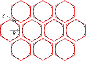
Figure 2: Sketch of close-packing arrangement. The maximum area fraction $f_{max}$ is obtained for $S=0$, and coincides with the ratio of the circle to hexagon area: $f_{max}=\pi/(2\sqrt{3})\simeq 0.91$. The deviation $f_{max}-f$ is the surface fraction of the interstices among the hexagons, which, for $S\ll R$, is $\propto S/R$.

The wave velocity field at the surface, $U_{x}(x,t)$, is horizontally compressible. The disk separation $S$ will thus oscillate in space and time, and, if $S$ is initially small, collisions will occur. Such collisions take place in the compression regions where $\partial_{x}U_{x}(x,t)<0$. If rafting is neglected, the disks will remain locked in their position relative to neighbours until $\partial_{x}U_{x}(x,t)$ becomes positive again. In such compression regions the wave will not see the disks as individual entities, rather as horizontally rigid agglomerates (“islands”) whose extension $\Delta$ scales with the wavelength $\lambda$.

We can try to be more quantitative on this.

The wave field at $z=0$,

$$U_{x}(x,t)=\frac{\mathcal{A}g}{\omega}\cos(kx-\omega t+\varphi),$$ (5.1)

where $2\mathcal{A}g/\omega^{2}$ is the crest to trough wave height, determines the motion of the disks. The relative motion of a pair of points separated by $X\ll\lambda$ in the $x$ direction obeys $\dot{X}\simeq X\partial_{x}U_{x}(x,t)$, which can be integrated to give

$$X(t)\simeq X(0)[1+\mathcal{A}\cos(kx-\omega t+\varphi)].$$ (5.2)

Consider two disks aligned along $x$, whose centers are separated initially by $X(0)\approx 2R$. The maximum relative displacement in a wave period will be $\approx R\mathcal{A}$ and the minimum rim to rim separation between neighboring disks, compatible with horizontal free motion in the wave field, will thus be $S\approx R\mathcal{A}$ (see Fig. 2).

Collisions among disks will take place in the regions of the wave in which

$$\mathcal{A}\cos(kx-\omega t+\varphi)>S/R$$ (5.3)

(see Eq. (5.2)). These regions are centered at the coordinates of instantaneous maximum compression $x_{l}=k^{-1}[\omega t-\varphi+(2l+1)\pi]$. Since in Eq. (5.3) $S/R\approx f_{max}-f$, the extension of these regions is independent of $R$ and scales with $\lambda$ as claimed,

$$\Delta=\frac{4}{\pi}\sqrt{\frac{\gamma}{11}}\lambda,\qquad\gamma=\gamma\Big{(}\frac{f_{max}-f}{\cal{A}}\Big{)},$$ (5.4)

where the proportionality coefficient is chosen to simplify the dispersion relation to be derived below. In the limit $f\to f_{max}$, we can imagine that islands coalesce to form a uniform layer, $\Delta/\lambda\to\infty$, corresponding to a peristaltic regime $U_{x}(x,t)=0$.

Arguments similar to those leading to Eqs. (3.17) and (3.18) can be used to estimate the stress perturbation under an island. The island’s structure can be likened to that of a lamellar armor, in which small metallic plates are laced into rows allowing flexibility in the normal direction. Of course this flexibility is lost when the length scale of the deformation (i.e. $\lambda$) is of the same order of the size of the lamellae (i.e. the disks, $R$).

For the tangential stress, the role of $R$ is replaced by $\Delta$:

$$\langle\tau_{xz}\rangle=\frac{11\mu\alpha\Delta^{2}}{64}\partial_{x}^{2}U_{x}\tanh(\hat{\alpha}\psi).$$ (5.5)

From Eq. (5.4), the expression for $\langle\tau_{xz}\rangle$ in Eq. (5.5) is $O(\epsilon_{k}^{-2})$ larger than the one in the first of Eq. (3.17).

If we assume that the disks remain free to move vertically as in the dilute case, the normal stress will continue to be generated by the resistance of the disks to bending. Thus, even if $\langle\pi_{zz}\rangle$ is going to be modified with respect to Eq. (3.17), its magnitude will be fixed by $R$ and will go to zero in the $\epsilon_{k},\delta/R\to 0$ limit of a continuous, horizontally homogeneous, but immaterial surface layer. This means that to leading order in $\epsilon_{k}$ the normal stress at the surface can be neglected.

It is interesting to note that in the present situation, the condition $\epsilon_{\alpha}\ll 1$ in Eq. (2.2) loses meaning and should be replaced by $\lambda_{\alpha}\ll\Delta$, which, for $\Delta\approx\lambda$, is always going to be satisfied.

We are now in the position to derive a dispersion relation in the close-packing regime, along the line of the procedure which leads to Eq. (4.13) in the dilute case. To allow comparison, at least in principle, with data from wave tank experiments, we allow $\hat{H}<\infty$.

Equation (4.6) for the tangential stress balance is then replaced by

$$(\gamma_{\psi}\hat{\nu}^{1/2}\hat{\alpha}\hat{k}+2\hat{\nu}\hat{k}^{2})\Phi^{\scriptscriptstyle U}_{+}+(\gamma_{\psi}\hat{\nu}^{1/2}\hat{\alpha}\hat{k}-2\hat{\nu}\hat{k}^{2})\Phi^{\scriptscriptstyle U}_{-}$$

$$-(1+2\hat{\nu}\hat{k}^{2})(A^{\scriptscriptstyle U}_{+}+A^{\scriptscriptstyle U}_{-})-\gamma_{\psi}\ (1-{\rm i}\hat{\nu}\hat{k}^{2})^{1/2}\ (A^{\scriptscriptstyle U}_{+}-A^{\scriptscriptstyle U}_{-})=0,$$ (5.6)

where $\gamma_{\psi}=\gamma\tanh\hat{\alpha}\psi$. We note that the disks contribute to the dynamics at $O(\hat{\nu}^{1/2})$ while in the dilute limit, they contribute only at $O(\hat{\nu})$.

Considering a finite depth regime implies that we must expand around $\hat{k}^{\scriptscriptstyle(0)}=\hat{k}_{\scriptscriptstyle H}$, that is the solution to the dispersion relation of gravity waves in a basin of depth $H$:

$$\hat{k}_{\scriptscriptstyle H}=q_{\scriptscriptstyle H}(\hat{k}_{\scriptscriptstyle H}).$$ (5.7)

This means that we must expand in Eq. (4.9)

$$q_{\scriptscriptstyle H-h}(\hat{k})=\hat{k}_{\scriptscriptstyle H}+(\hat{k}_{\scriptscriptstyle H}-\hat{k}^{\scriptscriptstyle(1)}\hat{H})(\hat{k}_{\scriptscriptstyle H}^{2}-1)\psi\hat{\nu}^{1/2}+\ldots$$ (5.8)

Putting to system Eq. (5.6) with Eqs. (4.7) to (4.9), and expanding the resulting secular equation to $O(\hat{\nu}^{1/2})$ gives the dispersion relation

$$\frac{\hat{k}}{\hat{k}_{\scriptscriptstyle H}}\simeq 1+\hat{\nu}^{1/2}\left\{\frac{{\rm i}\hat{\alpha}\gamma{\hat{\varrho}}\hat{k}_{\scriptscriptstyle H}^{2}\tanh(\hat{\alpha}\psi)}{(1+\gamma)[1+(\hat{k}_{\scriptscriptstyle H}^{2}-1)\hat{H}]}+\frac{(1-{\hat{\varrho}})(\hat{k}_{\scriptscriptstyle H}^{2}-1)\psi}{1+(\hat{k}_{\scriptscriptstyle H}^{2}-1)\hat{H}}\right\},$$ (5.9)

where the normal stress from the disks, that is $O(\hat{\nu})$, is disregarded. The second term in braces in Eq. (5.9) is the correction that would be produced by an inviscid layer of density different from the rest of the column, which is just a mass-loading effect (recall that $\psi\hat{\nu}^{1/2}=\hat{h}$, which is independent of $\nu$). The disks are accounted for by the first term in braces.

6 Discussion

6.1 The dilute theory

The theory has been derived for small $f$, $\epsilon_{\alpha}$, $\epsilon_{k}$ and $\delta/R$. The dispersion relation Eq. (4.13) accounts for the stresses by the viscous layer and by the disks, but not for the disks mutual interaction. In most situations involving pancake ice, such conditions are not fully satisfied. The dilute model can nevertheless be used in intermediate regimes, provided the pancake concentration is not too high and the locking mechanism described in the previous section does not set in. The situation as regards the other expansion parameters $\epsilon_{k}$ and $\epsilon_{\alpha}$ is not as dramatic and we expect that the theory is able to provide order of magnitude estimates also when the condition $\epsilon_{k,\alpha}\ll 1$ is not strictly satisfied.

An aspect that is worthwhile studying is the relative contribution by the viscous layer and by the disks to the wave dynamics. The two relevant limits Eqs. (4.14) and (4.16) of the dispersion relation Eq. (4.13) correspond to situations in which the stress by the disks and by the viscous layer, respectively, are dominant.

The magnitude of the contribution to the dispersion relation Eq. (4.13) from the stress by the viscous layer and from the tangential and normal stress components by the disks can be estimated as

$$O(\epsilon_{\alpha}^{3}\epsilon_{k}^{3}),\quad O(f\epsilon_{\alpha}\epsilon_{k}^{3})\quad{\rm and}\quad O(f\epsilon_{k}^{4}),$$ (6.1)

respectively.

Parameters typical of pancake ice in the ocean are $\nu=0.01\,{\rm m^{2}/s},\ R<1\,{\rm m}\ k_{\scriptscriptstyle\infty}=0.06\,{\rm m^{-1}}$), corresponding to $\epsilon_{\alpha}\approx 0.2$. To maximize the effect of the disks we set nominally $f=1$ in the analysis that follows.

As shown in Fig. 3, there are situations in which, even though $f=1$, the viscous layer dominates over the effect of the disks. This corresponds to the $\xi\to 0$ limit of Eq. (4.13), which is Eq. (4.16).

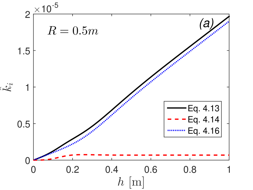
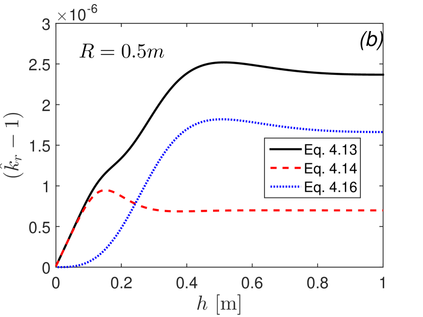
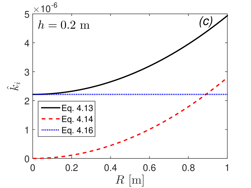
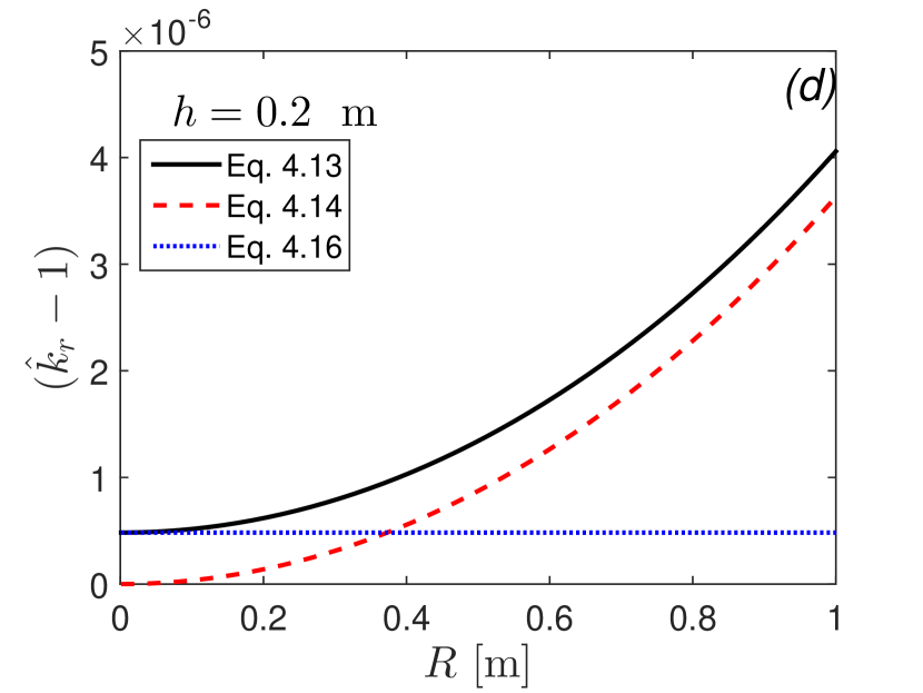
Figure 3: Plots of wave damping (panels (a) and (c)), and wave dispersion (panels (b) and (d)), in a typical pancake ice scenario. Values of the parameters: $\nu=10^{-2}\,{\rm m^{2}/s}$, $k_{\scriptscriptstyle\infty}=0.06\,{\rm m^{-1}}$, ${\hat{\varrho}}=0.917$, corresponding to $\lambda_{\alpha}=0.1142\,$m and $\hat{\nu}=4.69\cdot 10^{-5}$’. The choice $R=0.5$ m in panels ($a$) and ($b$) leads to $\xi=0.13$. The choice $h=0.2$ m in in panels $(c)$ and ($d$) leads to $\psi=1.75$. In all panels $f=1$.

The effect is more pronounced for damping than for dispersion. Inspection of Eq. (4.13) and of its limit forms tells us that the viscous layer’s effect is mainly damping of the waves, while the disks produce damping and dispersion that are of the same order. The damping by the viscous layer turns out to be larger than that by the disks ($\epsilon_{\alpha}$ is not small enough compared to the numerical coefficients in Eq. (4.13)). This implies that damping dominates over dispersion in most of the parameter range considered, and that the effect of the disks on wave damping is small. The effect decreases at larger $h$ and smaller $R$.

The situation is different as regards wave dispersion, as the viscous layer contribution to $\hat{k}_{r}-1$ is much smaller than to $\hat{k}_{i}$. This has the consequence that when the viscous layer is thin enough (less than $\approx\lambda_{\alpha}$ in thickness), the disks dominate dispersion.

The dispersion relation is drastically modified when $\epsilon_{k}$ and $\epsilon_{\alpha}$ are both small and $\xi=\epsilon_{k}/\epsilon_{\alpha}=O(1)$. Such a condition could be realized, in the range of $h$ and $R$ of Fig. 3, using a smaller viscosity. In the context of pancake ice, examples in which a smaller viscosity could be considered are generally related to the presence of oil: situations include oil spilling under pancake ice and oil incorporated into the ice as grease ice is formed (Fingas and Hollebone, 2003). We repeat in Fig. 4 the analysis in Fig. 3 adopting $\nu=10^{-4}\,{\rm m^{2}/s}$.

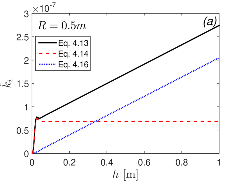
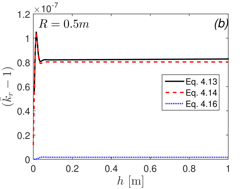
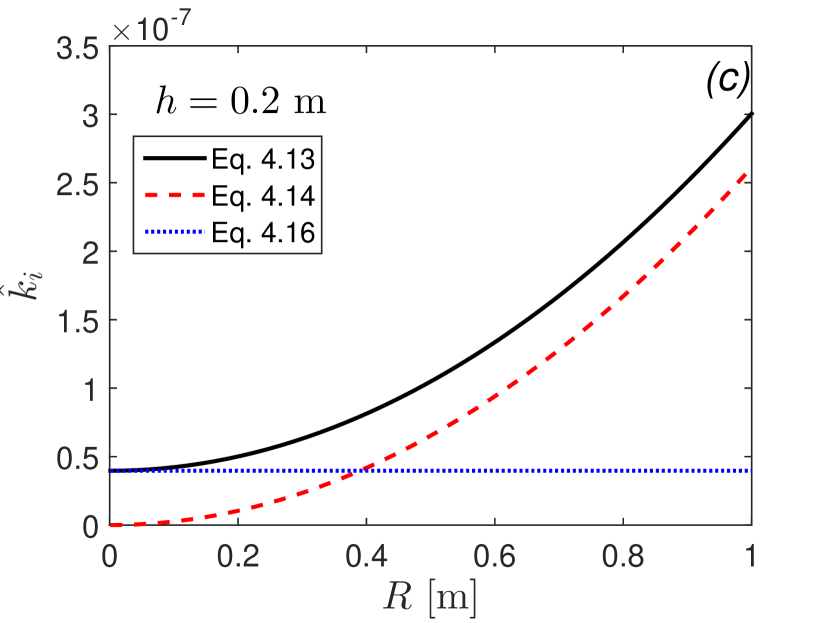
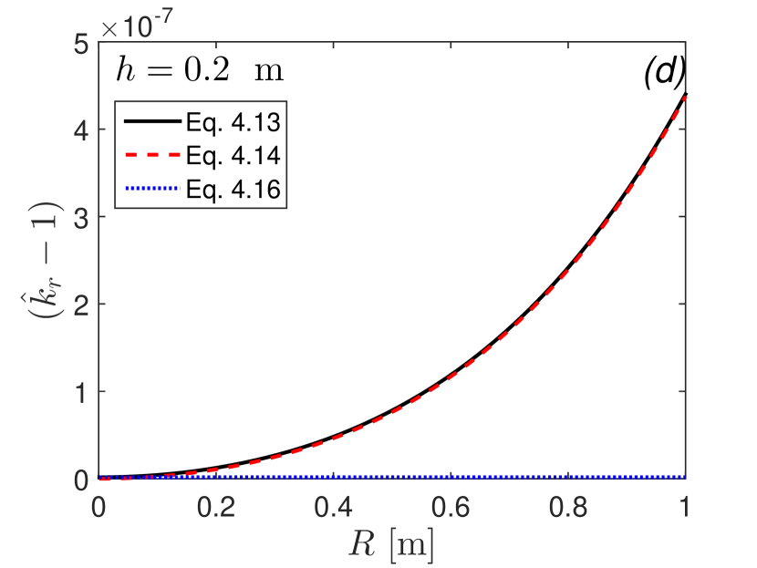
Figure 4: Plots of wave damping (panels (a) and (c)), and wave dispersion (panels (b) and (d)), in a possible pancake ice - mixed oil scenario. Effective viscosity $\nu=10^{-4}\,{\rm m^{2}/s}$; values of $k_{\scriptscriptstyle\infty}$, ${\hat{\varrho}}$ and $f$ as in Fig. 3.

In this case, we see that wave dispersion is dominated by the disks, while damping is dominated by the disks only for small $h$ and large $R$. In this parameter range, damping and dispersion are of the same order of magnitude. The slow dependence of the disk stress on $h$ is due to the fact that for small $\nu$, $\lambda_{\alpha}$ is small as well, $\psi$ is consequently large, and the tangential stress in Eqs. (3.17) and (3.18) reaches a plateau.

It is to be noted that the wave damping does not grow without bound for $\nu\to\infty$, instead, it first reaches a maximum for $h\sim\lambda_{\alpha}$, and then goes to zero for $\nu\to\infty$ (the first term in braces to RHS of Eq. (5.9) becomes purely real in the limit, with ${\rm i}\hat{\alpha}\tanh(\hat{\alpha}\psi)\simeq-\psi$). The limit corresponds to the viscous layer behaving as a rigid lid with the shape of the wave, which is transported by the wave itself. From analysis of Eq. (4.16), we see that the same limit cannot be achieved—within perturbation theory at least—in the case of a simple viscous layer.

6.2 The close-packing model

The model has been introduced to take into account the reduced relative mobility of the disks for $f\approx 1$. The dispersion relation Eq. (5.9), which is valid in the limit

$$R\ll\Delta,\lambda,$$ (6.2)

describes a situation in which both wave damping and dispersion are greatly increased with respect to the prediction of the dilute theory, for comparable values of the surface fraction $f$.

The dispersion relation Eq. (5.9) neglects normal stress contributions. Such contributions can be taken into account by an extended version of the model in which Eqs. (5.6) and (4.7) to (4.9) are solved without approximations. This reveals that the simplified model works well as long as $\Delta/R\gtrsim 4$ (see Fig. 5).

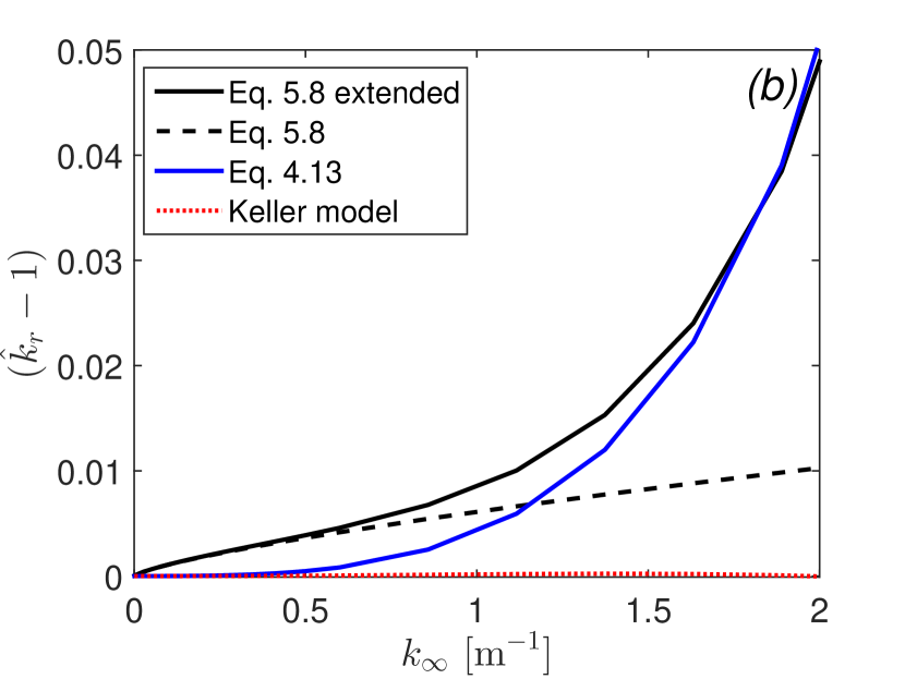
Figure 5: Comparison of the the predictions by the close-packing model and its extended version, the dilute theory and the Keller theory, in a typical pancake ice scenario. Values of the parameters: $\nu=10^{-2}\,{\rm m^{2}/s}$, ${\hat{\varrho}}=0.917$, $h=0.2\,$m, $R=0.5\,$m, $f=1$ and $\gamma=0.2$. Panel (a) wave damping; panel (b) dispersion.

For $\Delta\sim R$, the “extended” close-packing model merges with the dilute theory Eq. (4.13). As regards wave damping, we see in Fig. 5a that for a typical pancake ice scenario, with $\nu=0.01\ {\rm m^{2}/s}$, $R=0.5$ m and fixed $\gamma=O(1)$, this merging occurs for very short waves.

As regards wave dispersion, Fig. 5b illustrates that both Eqs. (4.13) and (5.9), and the extension of the second to $\epsilon_{k}\approx 1$, lead to a decrease of the phase velocity. As in the case of damping, the close-packing model gives a result that is orders of magnitude larger than that of the dilute theory at large wavelengths. We have included for reference the prediction by the Keller theory (Keller, 1998), which, for all values of $k_{\scriptscriptstyle\infty}$, disappears in front of the contribution from the pancakes in close packing conditions.

We can compare the results of the close-packing model with those of a viscoelastic model such as the one by Wang and Shen (2010a). The composite pancake-grease-ice layer is treated as a homogeneous Voigt medium with complex viscosity

$$\nu_{e}=\nu+\frac{{\rm i}G}{\varrho\omega}.$$ (6.3)

We take for the elastic modulus $G=10^{3}$ Pa (a value in the range of gels, but still much less than what would be observed in solid ice), and keep considering a shear viscosity typical of grease ice, $\nu=10^{-2}\ {\rm m^{2}/s}$. This choice guarantees that, in the small to moderate $k_{\scriptscriptstyle\infty}$ range considered, $\hat{\nu}_{e}=k_{\scriptscriptstyle\infty}^{3/2}g^{-1/2}\nu_{e}$ is small. The full dispersion relation, Eq. (45) in Wang and Shen (2010a), can then be approximated with our Eq. (4.16) by setting $H\to\infty$ and substituting $\hat{\nu}\to\hat{\nu}_{e}$.

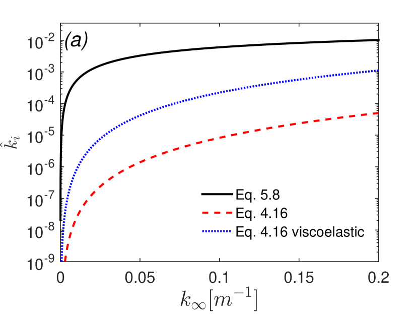
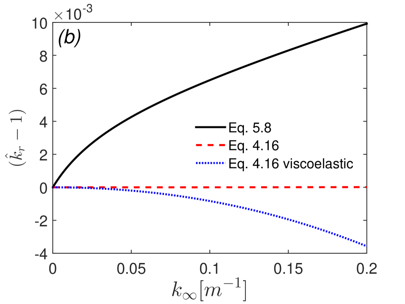
Figure 6: Comparison of the the predictions by the close-packing model, the viscous layer model and the viscoelastic layer model. Values of the parameters: $\nu=10^{-2}\,{\rm m^{2}/s}$, ${\hat{\varrho}}=0.917$, $h=0.2\,$m, $R=0.5\,$m, $\gamma=6$, $G=10^{3}\,{\rm Pa}$. Panel (a) wave damping; panel (b) dispersion.

As shown in Fig. 6, the viscoelastic model predicts a wave damping much smaller than the close-packing model, Eq. (5.9). Even smaller values of $\hat{k}_{i}$ are predicted in the purely viscous model, that is Eq. (4.16) in its original form with $\nu=0.01\ {\rm m^{2}/s}$ and $G=0$. The value of $\gamma$ adopted is close to the inextensible membrane limit; however, different choices do not produce dramatic modifications (see Fig. 5). The viscoelastic and close-packing model lead to values of the dispersion modification $\hat{k}_{r}-1$ of the same order of magnitude, although with opposite sign. Comparison with data from synthetic aperture radar imaginery by Wadhams and Holt (1991) (see Table 1 in that reference), suggest that $\hat{k}_{r}-1>0$ as in the close-packing model, even though it must be mentioned that such data referred to an inhomogeneous situation, in which regions with just grease ice and regions with grease and pancake ice were both present.

We have checked the validity of the close-packing model against some real field data on sea ice. We have considered the Bering Sea data of 7th February 1983 on wave damping reported by Wadhams et al. (1988). The data refer to waves propagating in ocean covered with ice floes of radius $R\approx 10$ m.

A fit of the data by Eq. (5.9) has been obtained for the reference value of the viscosity in the top layer $\nu=0.01\ {\rm m^{2}/s}$. The top layer viscosity may be due to the presence of grease ice, but in principle an eddy viscosity contribution may also be present due to the underwater stresses generated by the wind.

Best fit of Eq. (5.9) by least squares gives $h=0.14$ m, while $\gamma$ can take any value $\gtrsim 10$, corresponding to a peristaltic regime. Least square fit by the Keller model (Keller, 1998) varying $\nu$ and $h$, gives $\nu=10\ {\rm m^{2}/s}$ and $h=0.28$ m. In order for such a model to generate a wave damping of the same order of magnitude, a much larger value of the viscosity in the top layer must be adopted, which seems rather unrealistic.

Both models fail to predict the apparent rollover in the spectrum at $k_{\scriptscriptstyle\infty}>0.06\ {\rm m^{-1}}$.

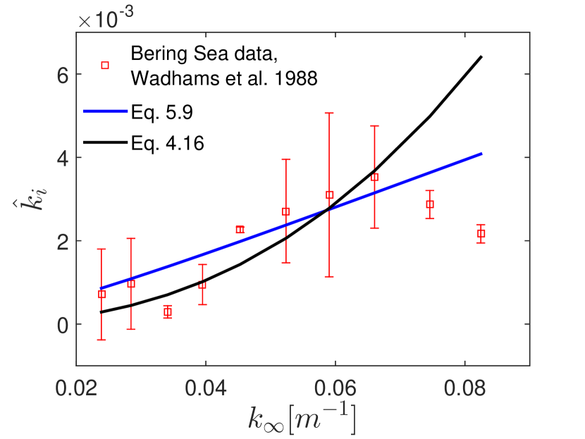
Figure 7: Comparison of field data on wave damping by ice floes ($R=10\,$m) (Wadhams et al., 1988) and prediction by the Keller model and close-packing model Eqs. (4.16) and (5.9). Values of the parameters: $\nu=0.01\,{\rm m^{2}/s}$, $h=0.14\,$m, $\gamma\to\infty$ (close-packing model); $\nu=10\,{\rm m^{2}/s}$, $h=0.21\,$m (Keller model).

7 Conclusion

We have studied the propagation of gravity waves in a water body covered by a distribution of thin disks embedded in a viscous layer. We have described the wave dynamics as a function of the surface fraction of the disks $f$, and of the relevant scales of the problem: the disk radius $R$; the wavelength $\lambda$; the depth $h$ of the viscous layer; the thickness $\lambda_{\alpha}$ of the viscous boundary layer at the surface (see Eq. (2.1)).

We have provided an analytical theory valid in the limit $\lambda_{\alpha}\ll R\ll\lambda$, $f\ll 1$. In such dilute limit, the interaction among disks is disregarded. In the range $\lambda_{\alpha}\lesssim h$, the role of control parameter is played by the quantity $\xi\sim R^{2}/(\lambda\lambda_{\alpha})$ defined in Eq. (4.5). In particular, the ratio of the normal and tangential stresses by the disks, and the ratio of the contribution from the disks and from the viscous layer to wave damping, are both proportional to $\xi$. It is interesting to note that, for values of the parameters compatible with pancake ice in the ocean (for which the dilute theory, however, would not work), the contribution to wave damping from the viscous layer would exceed that from the disks.

We have used the dilute theory as a groundwork for the development of a macroscopic model valid in a close-packing regime $f\approx 1$.

While in the dilute case, the surface stress is associated with surface strain rate on the scale of the individual disks, in the close-packing case it is the whole disk layer that resists horizontal compression. The result is a dramatic increase of the friction forces by the disks on the viscous layer, with wave damping and dispersion corrections larger by orders of magnitude than predicted by the dilute theory.

An interesting point in the close-packing model is the appearance of a new characteristic length $\Delta$, which represents the extension of the regions in which disks are so closely packed to form a horizontally rigid structure, and where tangential stress is maximum.

We have used the close-packing model to fit field data of wave propagation in ocean covered with ice floes (Wadhams et al., 1988, Wadhams and Holt, 1991). We have compared the performance of the model with that of the theory by Keller (1998). Using values of the parameters compatible with presence of a grease ice layer or possibly a turbulent boundary layer (effective viscosity $\nu=0.01\,{\rm m^{2}/s}$), we have observed that the data on wave damping reported by Wadhams et al. (1988) can be fitted reasonably well with the close-packing model. In comparison, the Keller theory would require much larger (and difficult to justify) values of the effective viscosity.

As far as wave dispersion is concerned, the close-packing model predicts a decrease of phase velocity, which seems to agree with the data by Wadhams and Holt (1991).

The close packing model fails to account for any rollover effect, which are predicted instead by nonlinear models such as the one by Shen and Squire (1998). In principle, nonlinear effects could be made to sneak in the close-packing model, by taking seriously the interpretation of $\Delta$ as the extension of the high compression regions of the wave field (the parameter $\gamma$ in Eq. (5.4) would become a function of ${\bf U}$). It is to be mentioned that rollover effects typically take place when the size of the disks is comparable to the wavelength, in which case our theory ceases to be meaningful. This prevents comparison with wave-tank data such as the ones in Wang and Shen (2010b). Similar limitations exist also with field data on wave damping in ice covered ocean, when large floes are present (Kohout et al., 2014).

Acknowledgements We wish to thank Peter Wadhams for suggestions in the initial phase of the work and Siddhanta Sabyasachi for helpfuld discussion. This research was supported by FP7 EU project ICE-ARC (Grant agreement No. 603887) and by MIUR-PNRA, PANACEA project (Grant No. 2013/AN2.02).

Appendix A Potential representation of time-dependent Stokes flows

We decompose the fluid velocity as

$${\bf u}=-\nabla\Phi+\nabla\times{\bf A}.$$ (A.1)

Assuming incompressibility, we have that $\Phi$ is potential

$$\nabla\cdot{\bf u}=0\Rightarrow\nabla^{2}\Phi=0.$$ (A.2)

The time-dependent Stokes equation is

$$\partial_{t}{\bf u}+\frac{1}{\varrho}\nabla P=\nu\nabla^{2}{\bf u}+\frac{1}{\varrho}{\bf f},$$ (A.3)

from which we get the vorticity equation

$$\partial_{t}[\nabla\times{\bf u}]=\nu\nabla^{2}[\nabla\times{\bf u}]$$ (A.4)

(we consider for simplicity the case in which the force field is of gradient type); in terms of potentials:

$$\partial_{t}[\nabla\nabla\cdot{\bf A}-\nabla^{2}{\bf A}]=\nu\nabla^{2}[\nabla\nabla\cdot{\bf A}-\nabla^{2}{\bf A}],$$ (A.5)

and, if we assume ${\bf A}$ divergenceless,

$$\partial_{t}\nabla^{2}{\bf A}=\nu\nabla^{2}\nabla^{2}{\bf A}.$$ (A.6)

Equation (A.6) has general solution ${\bf A}=\bar{\bf A}+{\bf A}^{\prime}$, where

$$\partial_{t}\bar{\bf A}=\nu\nabla^{2}\bar{\bf A},\qquad\nabla^{2}{\bf A}^{\prime}=0.$$ (A.7)

If we continue to assume that ${\bf A}$ is divergenceless, we see that ${\bf A}^{\prime}$ does not contribute to vorticity

$$\nabla\times[\nabla\times{\bf A}^{\prime}]=-\nabla^{2}{\bf A}^{\prime}=0.$$ (A.8)

We could decompose

$${\bf A}^{\prime}=\nabla q+\nabla\times{\bf C},\qquad\nabla^{2}q=0.$$ (A.9)

We have

$$\nabla^{2}{\bf A}^{\prime}=\nabla\times\nabla^{2}{\bf C}=0\Rightarrow\nabla^{2}{\bf C}=\nabla g,$$ (A.10)

which allows us to write the contribution of ${\bf A}^{\prime}$ to the velocity in the form

$$\nabla\times{\bf A}^{\prime}=\nabla(\nabla\cdot{\bf C}-g).$$ (A.11)

We see that adding a potential term ${\bf A}^{\prime}$ to the vector potential has the same effect as renormalizing the scalar potential:

$$\Phi\to\Phi+g-\nabla\cdot{\bf C}.$$ (A.12)

In general, the equation for the scalar potential will be

$$-\partial_{t}\nabla(\Phi+g-\nabla\cdot{\bf C})+\frac{1}{\varrho}\nabla P=\frac{1}{\varrho}{\bf f}.$$ (A.13)

The equation will simplify if ${\bf A}^{\prime}=0$, i.e. if we assume that ${\bf A}$ obeys the first of Eq. (A.7). In this case we shall have, taking ${\bf f}=-\nabla V$:

$$\partial_{t}\Phi=\frac{P+V}{\varrho}\quad{\rm and}\quad\partial_{t}{\bf A}=\nu\nabla^{2}{\bf A},$$ (A.14)

that are Eqs. (2.13) and (2.14).

Appendix B Green function of the potential component

It is convenient to expand the Neumann Green function, Eq. (2.29), in angular harmonics:

$$G^{N}({\bf r},\rho_{0})=\frac{2}{\sqrt{\rho^{2}+\rho_{0}^{2}}}\sum_{m=-\infty}^{+\infty}g_{m}^{N}\Big{(}\frac{r\rho_{0}}{\rho^{2}+\rho_{0}^{2}}\Big{)}{\rm e}^{{\rm i}m(\phi_{0}-\phi_{0}^{\prime})},$$ (B.1)

with

$$g^{N}_{m}(x)=\frac{1}{2\pi}\int_{0}^{2\pi}{\rm d}\phi\frac{{\rm e}^{-{\rm i}m\phi}}{\sqrt{1+x\cos\phi}}.$$ (B.2)

Thus

$$\Phi^{\scriptscriptstyle(0)}({\bf r})|_{z=0}=\sum_{m=-\infty}^{+\infty}\Phi^{\scriptscriptstyle(0)}_{m}(\rho,0){\rm e}^{{\rm i}m\phi_{0}},$$ (B.3)

where

$$\Phi^{\scriptscriptstyle(0)}_{m}(\rho,0)=-\int_{0}^{R}\rho_{0}\,{\rm d}\rho_{0}\ \frac{u^{\scriptscriptstyle(0)}_{m,z}(\rho_{0},0)}{\sqrt{\rho^{2}+\rho_{0}^{2}}}g^{N}_{m}\Big{(}\frac{\rho\rho_{0}}{\rho^{2}+\rho_{0}^{2}}\Big{)},$$ (B.4)

and similar expressions holding at higher orders. This allows to rewrite Eq. (3.8) as

$$\langle\pi_{xz}\rangle \simeq \frac{f\mu\alpha}{2\pi R}\frac{\partial^{2}\bar{U}_{x}}{\partial\bar{x}^{2}}\int_{0}^{2\pi}{\rm d}\phi\int_{0}^{R}\rho^{2}\,{\rm d}\rho\ \Big{[}\frac{\rho}{2R}(\cos^{4}\phi+\sin^{2}2\phi)\Big{]}$$ (B.5)

$$- \frac{f\mu\alpha}{4\pi}\frac{\partial^{3}\bar{U}_{z}}{\partial\bar{x}^{3}}\int_{0}^{2\pi}{\rm d}\phi\int_{0}^{R}\rho^{2}\,{\rm d}\rho\ \Big{\{}\cos^{2}\phi$$

$$\times \partial_{\rho}\int_{0}^{R}\rho_{0}{\rm d}\rho_{0}\ \frac{(\rho_{0}/R)^{2}-1}{\sqrt{\rho^{2}+\rho_{0}^{2}}}g^{N}_{0}\Big{(}\frac{\rho\rho_{0}}{\rho^{2}+\rho_{0}^{2}}\Big{)}+2\Big{(}\cos 2\phi\cos^{2}\phi\partial_{\rho}$$

$$+ \frac{\sin^{2}2\phi}{\rho}\Big{)}\int_{0}^{R}\rho_{0}\,{\rm d}\rho_{0}\ \frac{(\rho_{0}/R)^{2}-1}{\sqrt{\rho^{2}+\rho_{0}^{2}}}g^{N}_{2}\Big{(}\frac{\rho\rho_{0}}{\rho^{2}+\rho_{0}^{2}}\Big{)}\Big{\}}.$$

Carrying out the polar integrals and integrating by part in $R$ where necessary, we find

$$\langle\pi_{xz}\rangle \simeq \frac{11f\mu R^{2}\alpha}{64}\frac{\partial^{2}\bar{U}_{x}}{\partial\bar{x}^{2}}$$ (B.6)

$$- \frac{f\mu\alpha}{4}\frac{\partial^{3}\bar{U}_{z}}{\partial\bar{x}^{3}}\int_{0}^{R}\rho^{2}\,{\rm d}\rho\ \Big{\{}\partial_{\rho}\int_{0}^{R}\rho_{0}\,{\rm d}\rho_{0}\ \frac{(\rho_{0}/R)^{2}-1}{\sqrt{\rho^{2}+\rho_{0}^{2}}}g^{N}_{0}\Big{(}\frac{\rho\rho_{0}}{\rho^{2}+\rho_{0}^{2}}\Big{)}$$

$$+ \Big{(}\partial_{\rho}+\frac{2}{\rho}\Big{)}\int_{0}^{R}\rho_{0}{\rm d}\rho_{0}\ \frac{(\rho_{0}/R)^{2}-1}{\sqrt{\rho^{2}+\rho_{0}^{2}}}g^{N}_{2}\Big{(}\frac{\rho\rho_{0}}{\rho^{2}+\rho_{0}^{2}}\Big{)}\Big{\}}$$

$$= \frac{11f\mu R^{2}\alpha}{64}\frac{\partial^{2}\bar{U}_{x}}{\partial\bar{x}^{2}}-\frac{Bf\mu\alpha R^{3}}{2}\frac{\partial^{3}\bar{U}_{z}}{\partial\bar{x}^{3}},$$

with

$$B=\int_{0}^{1}\rho\,{\rm d}\rho\ \int_{0}^{1}\rho_{0}{\rm d}\rho_{0}\ \frac{1-\rho_{0}^{2}}{\sqrt{\rho^{2}+\rho_{0}^{2}}}g^{N}_{0}\Big{(}\frac{\rho\rho_{0}}{\rho^{2}+\rho_{0}^{2}}\Big{)}\simeq 0.16.$$ (B.7)

Appendix C Boundary conditions at the bottom of the viscous layer

The derivation of Eq. (4.8) is straightforward and is omitted. We concentrate on continuity of normal stress. We need first to enforce continuity of the normal velocity:

$$\Phi^{\scriptscriptstyle U}_{+}{\rm e}^{-kh}-\Phi^{\scriptscriptstyle U}_{-}{\rm e}^{kh}-{\rm i}(A^{\scriptscriptstyle U}_{+}{\rm e}^{-\alpha_{k}h}+A^{\scriptscriptstyle U}_{-}{\rm e}^{\alpha_{k}h})=\Phi^{\scriptscriptstyle U}_{w}\sinh[k(H-h)].$$ (C.1)

Continuity of normal stress gives

$$2\nu\partial_{z}U_{z}|_{z=-h^{+}}-P/\varrho=-P_{w}/\varrho.$$ (C.2)

The first of Eq. (2.13) allows us to write

$$P=\varrho\{-{\rm i}\omega(\Phi^{\scriptscriptstyle U}_{+}{\rm e}^{-kh}+\Phi^{\scriptscriptstyle U}_{-}{\rm e}^{kh})+\frac{{\rm i}gk}{\omega}\Phi^{\scriptscriptstyle U}_{w}\sinh[k(H-h)]\}$$ (C.3)

and

$$P_{w}=\varrho_{w}\Phi^{\scriptscriptstyle U}_{w}\{-{\rm i}\omega\cosh(k(H-h))+\frac{{\rm i}gk}{\omega}\sinh[k(H-h)]\}.$$ (C.4)

Substituting Eqs. (C.3) and (C.4) into Eq. (C.2), and passing to dimensionless variables, we get

$${\hat{\varrho}}({\rm i}-2\hat{\nu}\hat{k}^{2})(\Phi^{\scriptscriptstyle U}_{+}{\rm e}^{-\hat{k}\hat{h}}+\Phi^{\scriptscriptstyle U}_{-}{\rm e}^{\hat{k}\hat{h}})+2{\rm i}{\hat{\varrho}}\hat{\nu}^{1/2}\hat{\alpha}\hat{k}(A^{\scriptscriptstyle U}_{+}{\rm e}^{-\hat{\alpha}_{k}\psi}-A^{\scriptscriptstyle U}_{-}{\rm e}^{\hat{\alpha}_{k}\psi})$$

$$-{\rm i}\{q_{\scriptscriptstyle H-h}-(1-{\hat{\varrho}})\hat{k}\}\Phi^{\scriptscriptstyle U}_{w}\sinh[\hat{k}(\hat{H}-\hat{h})]=0,$$ (C.5)

where $q_{\scriptscriptstyle H-h}=1/\tanh[k(H-h)]$. We can eliminate $\Phi^{\scriptscriptstyle U}_{w}$ using Eq. (C.1), to obtain

$$\{{\rm i}[{\hat{\varrho}}-q_{\scriptscriptstyle H-h}+(1-{\hat{\varrho}})\hat{k}]-2{\hat{\varrho}}\hat{\nu}\hat{k}^{2}\}\Phi^{\scriptscriptstyle U}_{+}{\rm e}^{-\hat{k}\hat{h}}+\{{\rm i}[{\hat{\varrho}}+q_{\scriptscriptstyle H-h}-(1-{\hat{\varrho}})\hat{k}]-2{\hat{\varrho}}\hat{\nu}\hat{k}^{2}\}\Phi^{\scriptscriptstyle U}_{-}{\rm e}^{\hat{k}\hat{h}}$$

$$+[(1-{\hat{\varrho}})\hat{k}-q_{\scriptscriptstyle H-h}+2{\rm i}{\hat{\varrho}}\hat{\nu}^{1/2}\hat{\alpha}\hat{k}]A^{\scriptscriptstyle U}_{+}{\rm e}^{-\hat{\alpha}_{k}\psi}$$

$$+[(1-{\hat{\varrho}})\hat{k}-q_{\scriptscriptstyle H-h}-2{\rm i}{\hat{\varrho}}\hat{\nu}^{1/2}\hat{\alpha}\hat{k}]A^{\scriptscriptstyle U}_{-}{\rm e}^{\hat{\alpha}_{k}\psi}=0,$$ (C.6)

that is Eq. (4.9).

References

- Bennetts and Squire (2009) LG Bennetts and VA Squire. Wave scattering by multiple rows of circular ice floes. Journal of Fluid Mechanics, 639:213–238, 2009.
- Brekke and Solberg (2005) Camilla Brekke and Anne HS Solberg. Oil spill detection by satellite remote sensing. Remote sensing of environment, 95:1–13, 2005.
- De Carolis and Desiderio (2002) Giacomo De Carolis and Daniela Desiderio. Dispersion and attenuation of gravity waves in ice: a two-layer viscous fluid model with experimental data validation. Physics Letters A, 305:399–412, 2002.
- de Carolis et al. (2005) Giacomo de Carolis, Piero Olla, and Luca Pignagnoli. Effective viscosity of grease ice in linearized gravity waves. Journal of Fluid Mechanics, 535:369–381, 2005.
- Doble et al. (2015) Martin J Doble, Giacomo De Carolis, Michael H Meylan, Jean-Raymond Bidlot, and Peter Wadhams. Relating wave attenuation to pancake ice thickness, using field measurements and model results. Geophysical Research Letters, 42:4473–4481, 2015.
- Fingas and Hollebone (2003) MF Fingas and BP Hollebone. Review of behaviour of oil in freezing environments. Marine Pollution Bulletin, 47:333–340, 2003.
- Foldy (1945) Leslie L Foldy. The multiple scattering of waves. i. general theory of isotropic scattering by randomly distributed scatterers. Physical Review, 67:107, 1945.
- Jackson (1999) John David Jackson. Classical electrodynamics. Wiley, 1999.
- Keller (1998) Joseph B Keller. Gravity waves on ice-covered water. Journal of Geophysical Research: Oceans, 103:7663–7669, 1998.
- Kohout and Meylan (2008) AL Kohout and MH Meylan. An elastic plate model for wave attenuation and ice floe breaking in the marginal ice zone. Journal of Geophysical Research: Oceans, 113:C09016, 2008.
- Kohout et al. (2014) AL Kohout, MJM Williams, SM Dean, and MH Meylan. Storm-induced sea-ice breakup and the implications for ice extent. Nature, 509:604–607, 2014.
- Lamb (1932) Horace Lamb. Hydrodynamics. Cambridge university press, 1932.
- Longuet-Higgins (1953) Michael S Longuet-Higgins. Mass transport in water waves. Philosophical Transactions of the Royal Society of London A: Mathematical, Physical and Engineering Sciences, 245:535–581, 1953.
- Meylan (2002) Michael H Meylan. Wave response of an ice floe of arbitrary geometry. Journal of Geophysical Research: Oceans, 107:3005, 2002.
- Mosig et al. (2015) Johannes EM Mosig, Fabien Montiel, and Vernon A Squire. Comparison of viscoelastic-type models for ocean wave attenuation in ice-covered seas. Journal of Geophysical Research: Oceans, 120:6072–6090, 2015.
- Newyear and Martin (1999) Karl Newyear and Seelye Martin. Comparison of laboratory data with a viscous two-layer model of wave propagation in grease ice. Journal of Geophysical Research: Oceans, 104:7837–7840, 1999.
- Shen and Squire (1998) Hayley H Shen and Vernon A Squire. Wave damping in compact pancake ice fields due to interactions between pancakes, volume 74 of Antarctic Science Series, pages 343–351. American Geophysical Union, 1998.
- Squire (2007) VA Squire. Of ocean waves and sea-ice revisited. Cold Regions Science and Technology, 49:110–133, 2007.
- Squire and Williams (2008) VA Squire and TD Williams. Wave propagation across sea-ice thickness changes. Ocean Modelling, 21:1–11, 2008.
- Squire et al. (1995) Vernon A Squire, John P Dugan, Peter Wadhams, Philip J Rottier, and Antony K Liu. Of ocean waves and sea ice. Annual Review of Fluid Mechanics, 27:115–168, 1995.
- Wadhams et al. (2002) P Wadhams, F Parmiggiani, and G De Carolis. The use of sar to measure ocean wave dispersion in frazil-pancake icefields. Journal of physical oceanography, 32:1721–1746, 2002.
- Wadhams et al. (2004) P Wadhams, FF Parmiggiani, G De Carolis, D Desiderio, and MJ Doble. Sar imaging of wave dispersion in antarctic pancake ice and its use in measuring ice thickness. Geophysical research letters, 31:L15305, 2004.
- Wadhams (1973) Peter Wadhams. Attenuation of swell by sea ice. Journal of Geophysical Research, 78:3552–3563, 1973.
- Wadhams and Holt (1991) Peter Wadhams and Benjamin Holt. Waves in frazil and pancake ice and their detection in seasat synthetic aperture radar imagery. Journal of Geophysical Research: Oceans, 96:8835–8852, 1991.
- Wadhams et al. (1988) Peter Wadhams, Vernon A Squire, Dougal J Goodman, Andrew M Cowan, and Stuart C Moore. The attenuation rates of ocean waves in the marginal ice zone. Journal of Geophysical Research: Oceans, 93:6799–6818, 1988.
- Wang and Shen (2010a) Ruixue Wang and Hayley H Shen. Gravity waves propagating into an ice-covered ocean: A viscoelastic model. Journal of Geophysical Research: Oceans, 115:C06024, 2010a.
- Wang and Shen (2010b) Ruixue Wang and Hayley H Shen. Experimental study on surface wave propagating through a grease–pancake ice mixture. Cold Regions Science and Technology, 61:90–96, 2010b.
- Wang and Shen (2011) Ruixue Wang and Hayley H Shen. A continuum model for the linear wave propagation in ice-covered oceans: An approximate solution. Ocean Modelling, 38:244–250, 2011.
- Weber (1987) Jan Erik Weber. Wave attenuation and wave drift in the marginal ice zone. Journal of physical oceanography, 17:2351–2361, 1987.