The CHIANTI Atomic Database

Abstract

The CHIANTI atomic database was first released in 1996 and has had a huge impact on the analysis and modeling of emissions from astrophysical plasmas. The database has continued to be updated, with version 8 released in 2015. Atomic data for modeling the emissivities of 246 ions and neutrals are contained in CHIANTI, together with data for deriving the ionization fractions of all elements up to zinc. The different types of atomic data are summarized here and their formats discussed. Statistics on the impact of CHIANTI to the astrophysical community are given and examples of the diverse range of applications are presented.

1 Introduction

The CHIANTI atomic database was first released in 1996 [1] in time for the launch of the Solar and Heliospheric Observatory (SOHO; Domingo et al. [2]). This mission contained three ultraviolet spectrometers, and there was a community need for a freely-available atomic database and software package that would enable researchers to apply the latest atomic data-sets to analyze these data. The solar vacuum ultraviolet spectrum (roughly 100–2000 Å) is rich in emission lines formed over the temperature range $10^{4}$–$10^{7}$ K, and much activity took place from the 1960’s through to the 1980’s in first identifying these lines and then calculating atomic data that could be used to interpret the lines. By the early 1990’s atomic data were available for most of the abundant ions, yet the data and software to compute emissivities were not easily accessible to most researchers. K. Dere (Naval Research Laboratory, USA), H. Mason (Cambridge University, UK) and B. Monsignori-Fossi (Arcetri Observatory, Italy) devised an atomic database that would be freely-available to the community with software written in the Interactive Data Language (IDL) that was, and still is, widely used in Solar Physics. Since 1996 the CHIANTI database has continued to expand, including detailed coverage of the X-ray wavelength region (1–100 Å), atomic data for computing the ionization balance of electron-ionized plasmas, and a new Python-based software package. Version 8 of CHIANTI was released in September 2015 [3] and features many new data-sets that have resulted from recent large-scale atomic calculations, with particular focus on the coronal iron ions.

The present article describes the database and demonstrates the scope and impact of the project. A summary of each of the data-sets currently in CHIANTI is given, and examples of applications are discussed.

2 Scope and impact

CHIANTI contains atomic data for positively-charged ions and neutrals and Figure 1 shows the species currently found in the database. Successive versions of CHIANTI have both expanded the coverage of the database and increased the sizes of the atomic models. As illustrated by the pink boxes in Figure 1 a significant amount of effort has been expended in providing large atomic models for the coronal iron ions (Fe viii–xxiv) that are critical for many studies in astrophysics.

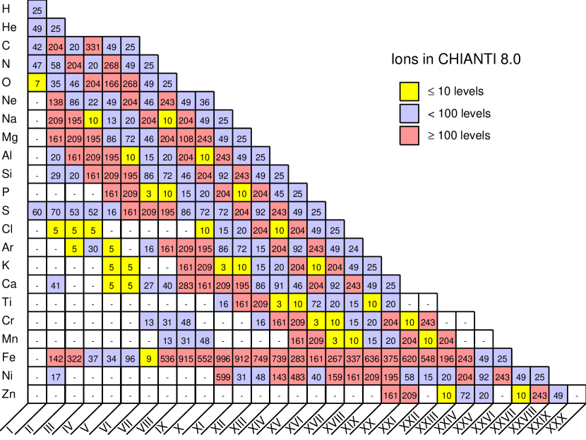
Figure 1: A table showing the elements and ions in CHIANTI 8. The number in each box indicates the number of atomic levels in the CHIANTI model for that ion. CHIANTI contains elements up to zinc, and low abundance elements such as Li, Be and B are not included.

The need for detailed atomic models for the iron ions is illustrated in Figure 2, which shows an observed quiet Sun spectrum from Manson [4] in the wavelength region 70–106 Å. Following the addition of new atomic data for the $n=4$ levels of the coronal iron ions and new line identifications by Del Zanna [5] in CHIANTI 8 [3] there is now much improved agreement with the observed spectrum. This wavelength region is now mostly complete in terms of atomic transitions, however many of the emission lines only have theoretical wavelengths.

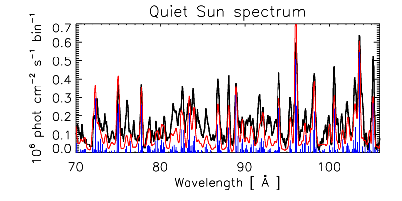
Figure 2: The black line shows an observed quiet Sun spectrum [4], and the red line shows the synthetic CHIANTI spectrum. Blue lines show the locations of the strongest transitions.

2.1 Data assessment

The CHIANTI team provide a single atomic model for each species in the database, with the best atomic data selected from the published literature. The assessment process is therefore a crucial component of the team’s work, and we identify three key elements:

1. graphical assessment of electron excitation collision strengths;

2. comparisons of new data-sets with previous data-sets; and

3. benchmark comparisons of emission line emissivities against observed spectra.

The electron collision strengths are the most important data-set in CHIANTI and a graphical procedure is applied to each atomic transition in order to identify anomalies such as typographic errors, discontinuities and, most critically, that the data points tend to the high temperature limit (see Sect. 4.2 and Dere et al. [1]). Where multiple data-sets are available, or a new data-set is being considered, then parameters are compared with a particular focus on the most important transitions for the ion.

The CHIANTI team have performed many benchmark studies to assess the accuracy of the atomic models, which serve both to validate the models and also to identify areas where improved data are required. The assessments include detailed analyses of specific solar spectra, such as those performed by Young et al. [6], Landi et al. [7], Landi & Phillips [8], Landi & Young [9], Young & Landi [10] and Del Zanna [11]. In addition benchmark studies for the coronal iron ions have been performed by Del Zanna [12], Del Zanna [13], Del Zanna et al. [14], Del Zanna [15], Del Zanna & Mason [16], and Del Zanna [17] for ions Fe vii–xiii, respectively.

2.2 Impact of CHIANTI

One measure of the success of CHIANTI is the number of citations the CHIANTI papers have received. There are 14 papers in all, nine of which describe the database and its updates, and the remaining papers present comparisons of CHIANTI with observed spectra. As of 2015 September 11, the CHIANTI papers had received 2091 citations from 1606 unique papers, and the number of citations with time is shown in Figure 3. An indication of the range of applications of CHIANTI can be made by identifying the most commonly-used keywords used by papers citing the CHIANTI papers, and these are shown in Figure 4. “Sun” is the most common, reflecting CHIANTI’s origins in the Solar Physics community, but “Stars” and “Astrophysics” are also prominent. We also highlight the large number of occurrences for both “X-rays” and “Gamma rays” reflecting the importance of CHIANTI for these areas even though CHIANTI was originally developed for modeling ultraviolet spectra.

Figure 3: The number of citations the CHIANTI papers have received as a function of time. The value for 2015 is an extrapolated value based on citations up to September.

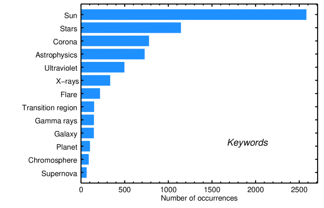
Figure 4: A histogram showing the most commonly-used keywords for papers citing the CHIANTI papers.

CHIANTI was originally designed for the needs of spectroscopists and it is now a widely-used tool for both solar and astrophysical spectroscopists. However CHIANTI is also used by many researchers in the plasma modeling community who need to be able to predict the radiative emissions from the plasma they model. Examples include the Hydrodynamic Radiation code (HYDRAD; [18, 19]) for modeling solar coronal loops, the Corona-Heliosphere code (CORHEL; [20]) and Alfven-Wave Solar Model (AWSoM; [21]) for modeling the global solar coronal emission, and the Radiative Transfer and Hydrodynamics code (RADYN; [22]) code for modeling solar and stellar flares. Astrophysics modeling codes that use CHIANTI include TARDIS for modeling emission from supernovae [23], the Monte Carlo Simulations of Ionised Nebulae (MOCASSIN) photoionization code [24], and the code of Richings et al. [25] for modeling the chemistry of the interstellar medium in galaxy simulations. The quality of the atomic data in CHIANTI has been recognised by other plasma codes that often choose to directly ingest the CHIANTI atomic data. Examples, include Cloudy [26], XSTAR [27] and ATOMDB [28].

Another use of CHIANTI is by space instrument teams who use it for deriving instrument response functions or for calibrating their instruments. An example is the Atmospheric Imaging Assembly (AIA; [29]) on board the Solar Dynamics Observatory (SDO; [30]) which obtains high resolution images of the Sun at ultraviolet and extreme ultraviolet wavelengths through narrow-band imaging. The response of the instrument’s filters to the plasma temperature depends on the spectral content of the bandpasses and for these CHIANTI is used [31]. The radiometric calibration of spectrometers can be checked by using the spectra themselves, for example certain ratios are known to be insensitive to plasma conditions. Revisions to the calibration of the EUV Imaging Spectrometer (EIS; [32]) on board the Hinode spacecraft [33] were made by Del Zanna [34] and Warren et al. [35] by making use of the CHIANTI database.

3 Level balance within an ion

Ions in low-density astrophysical plasmas are mostly in their ground electronic state and they are occasionally excited through collisions with free electrons. The excited states decay almost immediately back towards the ground through spontaneous radiative decay with the emission of photons. The situation is complicated by metastable levels and cascading. Metastable levels are mostly found within the ion’s ground configuration and they gain significant population with increasing density, providing additional excitation routes. Cascading is the process by which a level decays towards the ground level not in a single jump, but via other excited states. As two distinct atomic processes are at work in the excitation-decay process then the system is not in thermodynamic equilibrium and so the level populations of the ion have to be modeled by detailed balance of all the levels together, with atomic rates required for all levels in the model.

An important simplification is that ionization and recombination processes are generally much less frequent that the excitation and decay processes, and so the ionization balance equations are treated separately from the level balance equations. So, although we need the quantity $N_{j}$, the number density of ions in a certain atomic state $j$, to compute an emission line’s intensity, we separately compute the quantity $n_{j}=N_{j}/\left(\sum_{j}N_{j}\right)$ from level balance equations that consider only processes affecting levels within the ion. The full quantity $N_{j}$ is computed later by including the results of the separate ionization balance equations.

The level balance equations are considerably more complex than the ionization balance equations, and the principal purpose of CHIANTI is to provide the atomic data for accurately solving these level balance equations. Electron excitation rates and spontaneous radiative decay rates are the principal data-sets, but there are additional processes that need to be included for many ions and these are described in later sections.

Collisionless processes are described by rates (units: s^-1) while collision processes are described by rate coefficients (units: cm³ s^-1) so, for example, the total number of transitions leaving a state $j$ to enter a lower state $i$ through radiative decays and electron de-excitations is $N_{j}A_{ji}+N_{j}N_{\rm e}C_{ji}$ where $N_{j}$ is the number density of particles in the atomic state $j$, $A_{ji}$ is the radiative decay rate, $N_{\rm e}$ is the electron number density and $C_{ji}$ is the electron rate coefficient. The level balance equation for the level $j$, assuming only radiative decay and electron excitation are the important processes, is:

$$\sum_{k>j}N_{k}A_{kj}+N_{\rm e}\sum_{i\neq j}N_{i}C_{ij} = \sum_{i<j}N_{j}A_{ji}+\sum_{k\neq j}N_{j}N_{\rm e}C_{jk}$$ (1)

$${\rm[population~{}into~{}level}~{}j = {\rm population~{}out~{}of~{}level}~{}j]$$ (2)

In practice, for any specific level many of the terms in this equation will be zero or negligible. For example, an excited, non-metastable level will have radiative decay rates orders of magnitude larger than upwards or downwards electron excitation rates and so the latter will be negligible. For an excited metastable level in the ground configuration, however, many of the rates will be comparable in size and so all processes have to be included.

Solving the level balance equations yields the set of $n_{j}$ values for a specified electron number density and temperature ($T$), and the emissivity of an emission line resulting from a $j\rightarrow i$ decay occuring within an ion X^+q of element X is written as

$$\epsilon_{ij}(N_{\rm e},T)={N({\rm X})\over N_{\rm H}}{N_{\rm H}\over N_{\rm e}}{N({\rm X}^{+q})\over N({\rm X})}E_{ij}N_{\rm e}n_{j}A_{ji}\quad\quad{\rm erg~{}cm}^{-3}~{}{\rm s}^{-1}$$ (3)

where $N$ denotes the number density of the relevant species and $E_{ij}$ is the energy separation of the two atomic levels. This equation is often rewritten as:

$$\epsilon_{ij}(N_{\rm e},T)=G(N_{\rm e},T)N_{\rm e}^{2}$$ (4)

where $G$ is the contribution function. Tables of the element abundance relative to hydrogen, $N(X)/N_{\rm H}$, from various sources are provided in CHIANTI. The ionization fractions, $N({\rm X}^{+q})/N({\rm X})$, often written as $F(T)$, are computed from ionization and recombination rates stored in CHIANTI and a table of values for a wide range of temperatures is distributed in the database (see Sect. 6 for more details). The hydrogen to electron ratio, $N_{\rm H}/N_{\rm e}$, is calculated in a self-consistent manner using the abundance and ion fraction tables in CHIANTI. From the emissivities, synthetic spectra can be computed by assuming a model of the density and temperature structure of the plasma. See Phillips et al. [36] and the CHIANTI User Guide for more details.

In addition to the atomic data, CHIANTI contains a comprehensive software package for computing the quantities described above. For the original database the software was written in the Interactive Data Language (IDL), and this continues to be maintained to the present. In 2010 a version of the software written in the Python language was introduced and called ChiantiPy and this is maintained alongside the IDL version. Brief descriptions of each software package are given below.

3.1 IDL software

The CHIANTI IDL software routine pop_solver solves the matrix equations describing the level balance processes yielding the $n_{j}$ values discussed above. The contribution function is computed using the routine gofnt. Synthetic spectra are created with the graphic user interface routine ch_ss, which calls the lower level routines ch_synthetic and make_chianti_spec. Line ratio diagnostics are a crucial component of UV spectroscopy and these can be studied with the routines dens_plotter and temp_plotter for density and temperature diagnostics, respectively. For multi-thermal plasmas a differential emission measure describes the distribution of plasma with temperature, and the CHIANTI routine chianti_dem enables this to be computed. Further information about the IDL software is available in the CHIANTI user guide.

3.2 Python software

The ChiantiPy software package is written in Python (https://www.python.org), a free, modern, object-oriented computer language. ChiantiPy provides the ability to use the CHIANTI database to calculate the emission properties of coronal plasmas. It does this largely through an object-oriented approach. The most basic class/object is the “ion”, and an example of how to create the object for C iv is

> import chianti.core as ch
> myC_4ion = ch.ion(’c_4’,temperature, density)

where the user has already specified the temperature and electron density. The “ion” object has methods such as populate, popPlot, intensity, intensityRatio, freeFree, freeBound, and spectrum, among others. One can calculate the level populations of the ion and plot them:

> myC_4ion.populate()
> myC_4ion.popPlot()

The values of the population are then stored in a dictionary myC_4ion.Population which is directly available to the user. Until the user deletes the object, it and all of its methods remain for further calculations.

There are three spectrum classes: “spectrum”, “mspectrum”, and “ipymspectrum”. These all calculate the emission spectrum as a function of temperature and density for a given wavelength and line shape filter. This is done through a collection of “ion” objects. “spectrum” is a single processor version and “mspectrum” and “ipymspectrum” are multiprocessor versions. “ipymspectrum” can run inside a Jupyter/IPython (http://ipython.org/) notebook or qtconsole. “mspectrum” can run in a Python script or in a simple Jupyter/IPython console.

Further documentation on ChiantiPy can be found at http://chiantipy.sourceforge.net and the software package can be downloaded from https://sourceforge.net/projects/chiantipy. In the near future, ChiantiPy will be moving to GitHub (https://github.com).

4 Database structure

The CHIANTI atomic data files are all plain ascii files lying under a top directory called dbase. The data files for ions are stored in directories such as dbase/o/o_6 for O vi. Each file has a name of the form o_6.[ext] and the complete list of possible file extensions, [ext], are given in Table 1.

Additional data-sets distributed with CHIANTI include: tables of commonly-used element abundance data-sets; a table of equilibrium ionization fractions; and data-sets for computing continuum emission. These are stored in the sub-directories abundance, ioneq and continuum of dbase.

The following sections discuss the different types of atomic data-set contained in CHIANTI.

Table 1: CHIANTI file types.

	Extension	Purpose
Level balance files
	ELVLC	Level identifications and energies
	SCUPS	Scaled effective collision strengths and dielectronic capture rates (for “d” files)
	WGFA	Decay rates, 2-photon rates, autoionization rates
	FBLVL	Configuration energies for free-bound continuum calculation
	PSPLUPS	Spline fits to proton rate coefficients
	RECLVL	Level-resolved radiative recombination rates
	CILVL	Level-resolved ionization rates
Ion balance files
	DIPARAMS	Spline fits to direct ionization cross-sections
	EASPLOM	Spline fits to excitation-autoionization cross-sections
	EASPLUPS	Spline fits to excitation-autoionization rates
	RRPARAMS	Fit parameters for radiative recombination rates
	DRPARAMS	Fit parameters for dielectronic recombination rates

4.1 Energy levels

The ELVLC files contain a list of fine structure levels for each ion, giving transition information and the observed and/or theoretical energy. Each level is assigned an integer index, with the ground level assigned 1, and these indices are used to identify the levels in other data files. A level is only included in the file if there exist excitation and decay data to enable the level’s population to be modeled.

There are two energy columns in the files: one for experimental energies and the other for theoretical energies. Both are given in units of cm^-1. The NIST database is the principal source of experimental energy values, although other values are used where necessary. There are often energy levels for which no experimental values are available and so for these theoretical values are used from published calculations. In some cases the theoretical values can be improved, e.g., if another level in the same multiplet has a known energy, and the CHIANTI team will compute a “best-guess” energy and insert this into the theoretical energy column.

The format of the ELVLC files was changed in CHIANTI 8 [3], giving a simpler structure to the files but retaining the same information.

4.2 Electron excitation rates

The electron excitation rates form the single most significant data-set in CHIANTI and it is the one to which the most effort is applied. The data are stored as effective collision strengths, $\Upsilon$, (often referred to simply as “upsilons”) a dimensionless number derived from the integral of the collision cross-section with the Maxwellian distribution. Sect. 4.2.1 of Phillips et al. [36] gives further details, including the expression that relates the $\Upsilon$ to the electron excitation rate coefficient, $C$, discussed earlier.

The effective collision strengths are not stored directly but instead a scaling is applied, converting $\Upsilon(T)$ to $\Upsilon_{\rm s}(T_{\rm s})$, where $T_{\rm s}$ is a scaled temperature taking values between 0 and 1, with 1 corresponding to $T=\infty$. The scaling formulae vary according to the type of the transition, and the types are identified in Table 2. Types 1–4 were introduced by Burgess & Tully [37], Type 5 was introduced in CHIANTI 3 [38], and Type 6 in CHIANTI 4 [39].

Table 2: SCUPS file transition types.

Index	Type
1	Allowed transitions
2	Forbidden transitions
3	Intercombination transitions
4	Allowed transitions with a small $gf$ value
5	Dielectronic recombination transitions
6	Proton rates

The scaled temperatures and upsilons are stored in the SCUPS files, and they include the values $\Upsilon_{\rm s}(0)$ and $\Upsilon_{\rm s}(1)$. The former are obtained by performing a backwards extrapolation in $T_{\rm s},\Upsilon_{\rm s}$ space. The infinite temperature point for dipole-allowed transitions has a well-defined value based on the transition energy and $gf$ value [37], and this is used for most ions. The high temperature limit for non-dipole allowed transitions can be calculated using the method of Burgess et al. [40] (see also Whiteford et al. [41]), but most electron collision calculations do not provide these data. Exceptions are the recent calculations performed for the Atomic Processes for Astrophysical Plasmas (APAP) network, e.g., Liang et al. [42].

Prior to CHIANTI 8 [3], 5-point or 9-point splines were fit to the scaled upsilon data but this method was abandoned as the splines could not reproduce the complete set of upsilons for some transitions, and so it was necessary to remove some data points in order to obtain a good fit. Usually the removed points were in the low temperature regime, and so did not affect rates for electron-ionized plasmas but they could be significant for photoionized plasmas. This change has resulted in the scaled upsilons being stored in new SCUPS files, replacing the older SPLUPS files.

Most of the electron excitation rates are for levels below the ionization threshold of the ion, but for many ions we also include a set of levels above the ionization threshold, corresponding to inner shell excitation. For example, for the lithium-like ions with ground configuration $1s^{2}2s$, we include levels of the form $1s2s2l$ ($l=s,p$) corresponding to an excitation of a $1s$ orbital. These excitations are important in generating X-ray satellite lines (see also Sect. 4.5).

For most modern data-sets atomic physicists provide collision cross-sections in the form of effective collision strengths that are directly input to CHIANTI after scaling. In some cases the collision strengths, $\Omega$ (often referred to as “omegas”), are provided as a function of energy, and these are integrated over a Maxwellian distribution by the CHIANTI team to yield the upsilons that are then input to CHIANTI.

4.3 Radiative decay rates, two-photon rates and autoionization rates

The second key data-set for CHIANTI are the spontaneous radiative decay rates (often referred to as “$A$-values”), which are essential for solving the level balance equations. The rates are stored in the CHIANTI WGFA files together with the weighted oscillator strengths ($gf$) and the wavelengths for the transitions. The wavelengths are computed using the energies from the ELVLC file. If either or both of the two levels involved in a transition have theoretical energies, then the wavelength is given as a negative number, which serves as a flag to the software to indicate that the wavelength may not be accurate.

In addition to the spontaneous radiative decay rates, the WGFA files are also used to store two other types of rate: two-photon decay rates for hydrogen and helium-like ions, and autoionization rates. The two-photon decays are discussed in Sect. 5.3 and enable two states in the hydrogen and helium-like ions to decay that otherwise would be strictly forbidden, or decay very weakly. They result in a continuum of emission discussed in Sect. 5.3, and they also need to be included in the level balance of the ions. The critical difference in terms of the entries in the WGFA file is that the two-photon decays are assigned a zero wavelength so that a spectral line emissivity does not arise from the transition, instead the emission is separately modeled via the two-photon continuum emissivity calculation (Sect. 5.3).

For many ions in CHIANTI we include atomic levels that lie above the ionization threshold of the ion as these are needed for modeling dielectronic recombination lines (principally for X-ray spectra modeling). These levels can decay by regular spontaneous radiative decay, but they can also decay through autoionization, i.e., spontaneous ejection of the outermost electron. In terms of the emissivity calculation of the ion, the autoionizations serve to reduce the population decaying to lower levels in the ion. As for the two-photon decays, an autoionization is represented with a zero wavelength for the transition. The autoionization rate is inserted in the same column as the $A$-value and identified as a transition direct to the ground state. The transition of an autoionizing level to the ground state may thus be represented twice in the WGFA file: once for the radiative decay, and again for the autoionization rate. For solving the level balance equations the two rates are summed, but only the radiative decay yields an emissivity value.

4.4 Proton excitation rates

Atomic levels can be excited by collisions with protons, but only if the energy separation of the levels is small, as first demonstrated for the ground transition of Fe xiv [43]. Even for cases where the proton rates are larger than the electron rates, the dominant excitation process will usually be cascading from higher levels and so proton rates generally do not have a critical importance for the level balance equations. Most proton rate calculations were performed in the 1970’s through to the 1990’s, and rates for CHIANTI were assessed and added in version 4 of the database [39].

The proton rates are stored in PSPLUPS files, which contain 5 or 9-point spline fits to the rate coefficients. Where possible the transitions were fit with one of the electron excitation fitting formulae (types 1–4 in Table 2), but for many it was necessary to perform a fit to the logarithm of the rates corresponding to a type 6 transition [39]. For any single ion the PSPLUPS files contain at most a handful of transitions.

4.5 Dielectronic capture

CHIANTI 3 [38] extended CHIANTI to the X-ray wavelength range and a particular focus was on the addition of satellite lines. As an example, consider the strong $1s^{2}$ ${}^{1}S_{0}$ – $1s2p$ ${}^{1}P_{1}$ transition of helium-like ions, and the transition $1s^{2}3d$ – $1s2p(^{1}P)3d$ in lithium-like ions. The latter is essentially the same transition as for the helium-like ion, only it takes place in the presence of a high-lying $3d$ electron. The $3d$ electron serves to make a perturbation to the wavefunctions of the two states, meaning the wavelength of the lithium-like transition will be close to the helium-like transition, hence it is referred to as a satellite line of the helium-like transition.

Continuing this example, the $1s2p(^{1}P)3d$ level lies above the ionization threshold and it is excited either by excitation of the inner $1s$ shell or by dielectronic capture of a free electron onto the helium-like system. The former case is a regular electron excitation and is included in the SCUPS file (Sect. 4.2). The latter is a different process and is treated in the following way.

A completely new set of ion models were introduced with CHIANTI 3 [38] that were identified by adding a “d” to the ion names. For example, “o_6d” for the dielectronic files of O vi. For each dielectronic ion model there is a ELVLC, WGFA and SCUPS file. The excitations in the SCUPS files are actually dielectronic excitations coming from the recombining ion and are fit as Type 5 transitions (Table 2 and [38]). They are considered as excitations from the ground level of the recombined ion, and only excitations to the doubly-excited states are included in the file. The WGFA file contains radiative decay rates and autoionization rates for de-populating the doubly-excited levels. Note that a full set of decay rates is needed in order to track the cascading through the ion’s level structure.

The dielectronic model produces a “second spectrum” for the ion containing both new lines and duplicates of lines in the main ion model. When computing the complete synthetic spectrum from a plasma, the CHIANTI software sums the two spectra, thus potentially enhancing lines from the original model.

4.6 Level-resolved ionization and radiative recombination rates

The processes of ionization and radiative recombination can leave the final ion in an excited state, thus providing an additional population component to the excited levels that enhances the intensities of emission lines from these levels. To model these processes correctly it would be necessary to develop models for the entire sequence of ions of an element and allow transitions between states in neighboring ions, rather than just within a single ion. This would be a significant change to the structure of CHIANTI, greatly increasing processing time for the CHIANTI software.

A convenient solution can be made in the case where the population of the ground state of an ion is much greater ($\sim$ a factor 100) than the population of any other state, and this was introduced in CHIANTI 5 [44] for the iron ions Fe xvii–xxiii and selected ions of the hydrogen and helium-like sequences.

Rather than include the ionization and recombination rates when computing the level balance equations, the rates are introduced as part of a correction factor applied to populations computed using the regular CHIANTI calculation. For the ions considered, the method is accurate up to densities of $\approx$ $10^{13}$ cm^-3.

The rate coefficients for the processes are stored in RECLVL and CILVL files for recombination and ionization, respectively, as a function of $\log\,T$. They are considered as “excitations” from the ground level.

We highlight that the recombination data stored in the RECLVL file are for radiative recombinations into bound levels of the ion. Recombinations into doubly-excited states of the ion are modeled through the dielectronic models of the ions (Sect. 4.5).

4.7 Photoexcitation and stimulated emission

In the presence of a radiation field the additional radiative processes of photoexcitation and stimulated emission can take place, however these do not require additional atomic data: the rates are computed using the radiative decay rates (Sect. 4.3) and a function representing the energy density distribution of the radiation field. CHIANTI 4 [39] introduced modifications to the CHIANTI software to allow the processes to be modeled assuming a blackbody radiation field. A further modification was introduced in CHIANTI 5 [44] to allow an arbitrary radiation field to be input.

5 Continuum emission

Continuum emission is important for high temperature astrophysical plasmas and for many years the standard reference for astronomers was the work of Mewe et al. [45], which is implemented in the IDL routine CONFLX. The three components to the continuum are free-free, free-bound and two-photon, although the latter is a minor contributor. The current CHIANTI implementations were introduced in CHIANTI 4 [39], and comparisons with Mewe et al. [45] were presented by Landi [46]. Data files for the continuum processes are stored in dbase/continuum.

5.1 Free-free

Free-free or bremsstrahlung emission occurs when a free electron is decelerated during a collision with a positively-charged ion, and it is typically implemented in spectral codes through tabulations of the free-free Gaunt factor. For CHIANTI we use the relativistic Gaunt factor tabulation of Itoh et al. [47], supplemented by the non-relativistic Gaunt factors of Sutherland [48] for parameter ranges not covered by Itoh et al. [47].

5.2 Free-bound

The free-bound emission results from the capture of a free electron by an atom or ion and the capture can take place into any bound level of the ion. The critical atomic parameter is the capture cross-section into a bound state $i$, although in practice the cross-section for the inverse process, photoionization, is computed with the two cross-sections related by the principle of detailed balance (the Milne relation). The expression relating the photoionization cross-sections to the free-bound emissivity is given in Eq. 12 of Young et al. [39].

For CHIANTI the photoionization cross-sections from the ground state are taken from Verner et al. [49], and for excited levels (i.e., excited levels in the recombined ion) the Gaunt factor expression of Karzas & Latter [50] is used. For this expression levels are treated as configurations, thus if the ground configuration is $3s^{2}3p^{2}$, then the excited configurations are $3s^{2}3pnl$ and Gaunt factors are available for $n$ up to 6 and $l$ up to 5. Energies for these configurations are stored in the CHIANTI .FBLVL files, which are available for each ion. See Young et al. [39] for more details.

The data files for the Verner et al. and Karzas & Latter data-sets are stored in dbase/continuum and IDL routines (verner_xs and karzas_xs) are available for deriving the photoionization cross-sections from these two data-sets.

5.3 Two-photon

The two-photon continuum arises from the decays of the $1s$ ${}^{2}S_{1/2}$ state in hydrogen-like ions, and the $1s2s$ ${}^{1}S_{0}$ state in helium-like ions. The transition from the helium-like state to the ground is strictly forbidden and so the two-photon decay is the only decay route, whereas the hydrogen-like state has a weak magnetic dipole decay to the ground but this is weaker than the two-photon decay rate for most ions.

The decay route in both cases is the simultaneous emission of two photons for which the summed energies correspond to the energy difference between the excited state and the ground. Other than this restriction, the photons can take any energy and thus a continuum results. The key atomic parameters are the decay rate and the spectral distribution function, which describes the distribution of photon energies for an ensemble of particles. These parameters are stored in data-files in the dbase/continuum directory of CHIANTI. More details are given in Young et al. [39].

The decay rates are also stored in the WGFA files as they are necessary for solving the level balance equations for the hydrogen and helium-like ions (see Sect. 4.3).

6 Ionization balance

The major additions to CHIANTI 6 were total ionization and recombination rates for all ions, allowing the equilibrium ionization balance of the plasma to be computed for any temperature. These equations simply need total rates between neighbouring ions along an element’s ionization sequence, and they yield the ionization fractions, $F(T)$, for each ion. Since ionization and recombination are electron collision processes then, to first order, there is no density dependence to the ionization fractions. However, as density increases then metastable level populations can become significant and give different routes for ionization and recombination to take place, modifying the total ionization and recombination rate coefficients. In addition, dielectronic recombination is known to be suppressed at high densities (e.g., Nikolić et al. [51]). For CHIANTI we assume the zero density approximation, and use total, density-independent ionization and recombination rates for determining the ion balance. Prior to the CHIANTI 6 update astrophysicists relied on occasional updates to the zero-density ionization balance calculations, the most well-known being those of Arnaud & Rothenflug [52], Arnaud & Raymond [53] and Mazzotta et al. [54]. The addition to CHIANTI allows the ionization fractions to be updated on the typical $\approx$ 2 year update schedule of the database, and researchers are recommended to use the CHIANTI calculations as these contain improved atomic data compared to the earlier calculations.

The formats for storing the recombination and ionization rates are described below.

6.1 Ionization rates

Ionization includes both direct ionization and excitation-autoionization. The parameters for calculating the direct ionization cross-sections are contained in the DIPARAMS file. Dere [55] developed a Burgess & Tully [37] type of scaling for direct ionization cross-sections. The data in these files are fits to the scaled energies and ionization cross-sections. These may be either experimental cross-sections or calculated cross-sections. The direct ionization from several shells can be important and this is reflected by fits to more than a single cross-section. For example, Fe xiii has a ground configuration of $2p^{6}3s^{2}3p^{2}$ and the DIPARAMS file contains fits to the three sets of cross-sections for ionizations of the $3p$, $3s$ and $2p$ orbitals. The total cross-section is obtained by summing these cross-sections. The direct ionization rate coefficients are obtained by a 12 point Gauss-Laguerre integration over a Maxwellian electron distribution. Full details are given by Dere [55].

Excitation-autoionization occurs when an electron collides with an ion and excites it into a state above the ionization potential. The ion in this state can undergo a stabilizing radiative transition, leaving it in a stable state of the original ion. If the excited ion undergoes autoionization then it is left in a stable state of the higher ionization stage. The parameters for calculating the ionization cross-section by excitation-autoionization are in the EASPLOM files. These contain Burgess-Tully fits to the excitation cross-sections multiplied by the branching ratio of the autoionization process appropriate for the excited state. The parameters for calculating the excitation-autoionization rate coefficients are developed by an integration over a Maxwellian velocity distribution. The results are stored as Burgess-Tully fits to the scaled rate coefficients. The parameters for calculating the ionization rate coefficients by excitation-autoionization are in the EASPLUPS files. Considering ionization of Fe xiii again, the excitation routes considered by Dere [55] are $n=2$ to $n=3$, 4 and 5, and so there are three entries in the EASPLOMS and EASPLUPS files.

6.2 Recombination rates

Recombination is the capture of an electron into a bound state of the recombined ion. The capture can take place either directly, or indirectly by capture to an unstable doubly-excited state of the recombined ion, followed by a radiative decay to a bound state. The two types are referred to as radiative and dielectronic recombination, respectively, and in terms of theoretical calculations they are usually computed separately. One exception is the method of Nahar & Pradhan [56] which computes the total recombination coefficient in a single calculation, however Pindzola et al. [57] have demonstrated that interference between the RR and DR processes is negligible, justifying the independent processes approach.

6.2.1 Radiative recombination

Radiative recombination (RR) data are stored in the RRPARAMS files, which contain a single set of fit parameters for the total RR rate coefficient. There are three types of fitting formulae used for RR rates which were introduced by Aldrovandi & Pequignot [58], Verner & Ferland [59], and Gu [60].

The bulk of the RR data used in CHIANTI are from recent calculations of N.R. Badnell and collaborators. Badnell [61] performed calculations for all elements up to zinc for all ions from bare nucleus to sodium-like. Further work for the magnesium, aluminium and argon sequences were performed by Altun et al. [62], Abdel-Nagy et al. [63] and Nikolić et al. [64], and data for additional iron ions were presented by Badnell [65] and Schmidt et al. [66]. Data for the remaining ions are mostly from older calculations and are summarized in Dere et al. [67].

6.2.2 Dielectronic recombination

Dielectronic recombination (DR) was described previously (Sect. 4.5) in regard to modeling the strength of satellite lines at X-ray wavelengths. For modeling the ionization balance the total DR rate coefficients are required and a recent project described by Badnell et al. [68] produced complete sets of rates for all ions up to zinc for all sequences from hydrogen-like to aluminium-like. Beyond these sequences there are few calculations in the literature and rates are mostly calculated with variants of the Burgess General Formula [69] or interpolation – see Dere et al. [67] for more details.

All DR rates are fit with a standard formula first given by Arnaud & Raymond [53], and the CHIANTI DRPARAMS file contains the fit parameters.

7 Applications

The previous sections described the contents of the CHIANTI database, and in this section we present five examples of the varied uses of CHIANTI within the solar physics community.

7.1 Density diagnostics

For many ions one can find pairs of emission lines that are sensitive to the electron density, a famous example being the O ii $\lambda$3729/$\lambda$3726 ratio (Seaton & Osterbrock [70]). Density diagnostics are among the most important applications of CHIANTI, and two examples are illustrated here from the Hinode/EIS and Interface Region Imaging Spectrometer (IRIS; [71]) missions.

One of the most important density diagnostics for the Hinode/EIS mission is Fe xii $\lambda$186.9/$\lambda$195.1 ($\lambda$186.9 is actually a blend of two close transitions) that is formed at 1.5 MK. The ratio yields very precise density measurements (Young et al. [72]) enabling high quality density maps of active regions, such as shown in Figure 5. Comparisons of densities in this active region with a typical quiet Sun data-set show that coronal loops in the periphery of the active region have a density $\approx$0.5 dex larger than quiet Sun, whereas bright “knots” of emission in the active region core can be 1.5–2.0 dex higher. Atomic data from CHIANTI 8 were used to derive the densities and the EIS calibration of Del Zanna [34] was used.

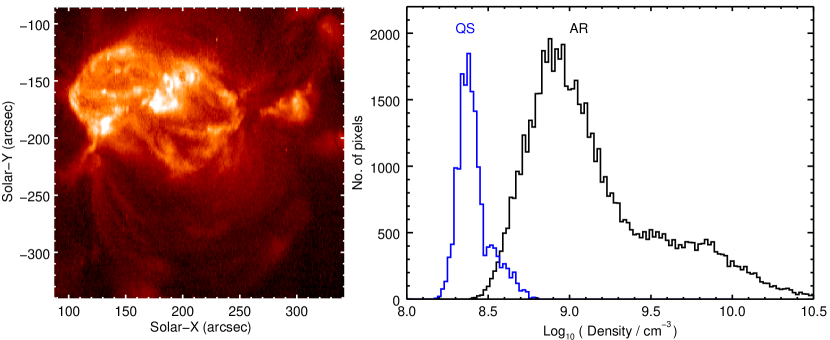
Figure 5: The left panel shows a density map with logarithmic scaling derived from an EIS raster beginning at 10:33 UT on 2006 December 2. The map is derived from Fe xii $\lambda$186.9/$\lambda$195.1. The right panel shows a histogram of the derived densities from the active region (AR). The blue histogram shows densities derived from the same ratio from a quiet Sun (QS) raster beginning at 12:15 UT on 2010 October 8.

O iv yields a set of five intercombination transitions between 1397 and 1407 Å that are widely used in both solar physics and astrophysics (e.g., Hayes & Shine [73]; Keenan et al. [74]). IRIS is the most recent UV instrument to measure these lines, and Figure 6 shows the theoretical variation of the O iv $\lambda$1399.8/$\lambda$1401.2 ratio obtained from CHIANTI 8 with observed ratio values from IRIS over-plotted. The measurements were obtained from a range of solar features (Young [75]), and the largest values are obtained from bright flare kernels, while the lowest value is obtained from a coronal hole. This plot demonstrates both that the diagnostic is very useful in a wide range of conditions, but also that the atomic data in CHIANTI allows accurate measurements of the density.

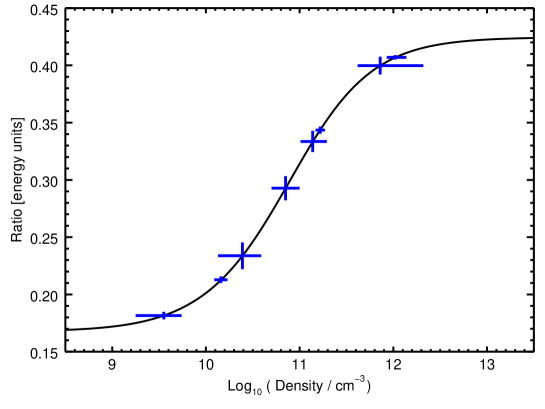
Figure 6: The solid line shows the theoretical variation of the O iv $\lambda$1399.8/$\lambda$1401.2 ratio as a function of density computed at $\log\,T=5.15$ using CHIANTI 8. The blue crosses show the measured ratios and densities with 2-$\sigma$ error bars. Figure adapted from Young [75].

7.2 Reponse functions for the SDO/AIA instrument

The AIA instrument on board the SDO satellite has seven EUV filters that pick out different wavelength regions in the solar spectrum, giving the instrument a wide temperature coverage (O’Dwyer et al. [76]). One of the filters is centered at 131 Å and CHIANTI is used by the AIA team to model the response of the filter to different solar conditions, as illustrated in Fig. 7. Panel a shows an image recorded from a solar flare that occurred at the solar limb. In these conditions the underlying solar spectrum, as modeled with CHIANTI, is shown in panel b. Although the strongest transition is Fe xxiii $\lambda$132.91, the instrument response function (shown in green) is low at this wavelength and the dominant transition is actually Fe xxi $\lambda$128.75, formed at 11 MK.

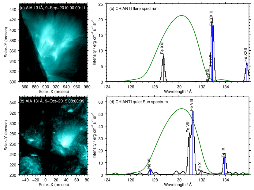
Figure 7: Panels a and c show images obtained with the AIA 131 Å filter, both displayed with a logarithmic intensity scaling. Panel a shows a flare at the solar limb, and panel c shows a bright plume within a low latitude coronal hole. Panels b and d show synthetic CHIANTI spectra for flare and quiet Sun conditions, respectively, with the AIA 131 Å response function over-plotted in green. The five strongest lines in each spectrum are indicated.

Fig. 7c shows an image obtained in a coronal hole, showing a number of plume structures. In these conditions the CHIANTI spectrum is as shown in Fig. 7d, with all of the hot flare lines absent and instead the dominant transitions come from Fe viii, formed at 0.8 MK.

7.3 Modeling of the solar corona

Modern computing power enables 3D magnetohydrodynamic (MHD) models of the solar corona to be constructed, and often CHIANTI is used to synthesize observed emissions from the models. An example is shown in Figure 8, which is taken from Peter [77] and uses the model presented by Peter et al. [78]. It shows a view from the top of the computational box which corresponds to an observation near the center of the solar disk. The left panel shows the line intensity as expected for Mg x (624.9 Å) originating from plasma at about 1 MK. Synthesising spectral line profiles at each grid point of the computational domain, line-of-sight integration (here along the vertical) provides a map of line profiles similar to what is acquired during a raster scan with a slit spectrograph. Fitting a single Gaussian to the line profiles then provides a Doppler map (right panel). At this particular instance in time a bright loop can be seen that hosts a siphon flow from the right to the left that shows up as a blueshift at the right and a redshift at the left leg of the loop (indicated by the dashed lines). The coronal emission was synthesised using an earlier version of CHIANTI (v4.02; Young et al. [39]).

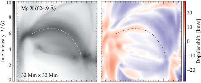
Figure 8: Coronal emission synthesised from a snapshot of a 3D MHD model of an active region. Courtesy of Hardi Peter.

7.4 Solar wind diagnostics

The solar wind plays a critical role in shaping the heliosphere and in determining the motion, arrival time and geo-effectiveness of Earth-directed coronal mass ejections (CMEs), and thus is a fundamental ingredient in Space Weather predictions. One of the main tools to investigate the properties, heating, acceleration and origin of the solar wind is the charge state composition measured in situ by space instrumentation. This quantity is determined by two key factors: 1) the evolution of the wind plasma velocity, electron density and temperature, and 2) the ionization and recombination rates of wind ions.

CHIANTI provides all the ionization and recombination data necessary to calculate the evolution of the ionization status of the plasma from the wind source region to the freeze-in point. This quantity can be used for several purposes. For example, Schwadron et al. [79] used the O⁷⁺/O⁶⁺ ratio to provide a crude estimate of the temperature of the solar corona, suggesting that the ratio decrease during solar cycle 23 indicated a global cooling of the solar corona. Edgar & Esser [80] and Ko et al. [81] compared predicted and observed charge state composition to study nonthermal electrons in the solar atmosphere; Esser & Edgar [82] used charge states to investigate differential velocities in the wind; and Ko et al. [83] and Esser et al. [84] used the measured oxygen charge state distribution to provide empirical models of the evolution of the wind velocity, electron density and temperature with distance from the source region.

CHIANTI has enabled a more accurate and comprehensive study of solar wind ionization by providing a compact database with the necessary rates. For example, Landi et al. [85] used CHIANTI-based calculation of the wind ionization status to systematically study departures from equilibrium in the wind plasma, finding that they are significant and affect spectral line emission even in the inner corona and so need to be taken into account. Landi et al. [86] showed that the radiative losses of the wind depart from equilibrium at transition region temperatures, altering the energy equation in solar wind models. Landi et al. [87] also devised a new diagnostic technique which is based on CHIANTI calculations of the wind plasma ionization to produce empirical models of the wind velocity, electron density and temperature; in this technique in-situ measurements of the wind charge state composition and remote sensing spectral observations of the wind source regions are compared with CHIANTI-based spectra and charge state distributions calculated under non-equilibrium ionization.

7.5 Applications to non-Maxwellian plasmas

The assumption of a Maxwellian distribution for the particle energies is fundamental to CHIANTI, encapsulated in the use of effective collision strengths and rate coefficients for the electron and proton collision processes (Sects. 4.2, 4.4 and 6). Extension to non-Maxwellians is possible if the distribution can be expressed as a linear combination of Maxwellians at different temperatures, and modifications to the CHIANTI software were performed in CHIANTI 4 [39] to enable this. An example of the use of the method was presented by Muglach et al. [88] who investigated how the effect of a high-temperature tail of electrons would modify emission line ratios.

An alternative approach was presented by Dzifčáková [89] who provided a method for deriving collision strengths integrated over a kappa distribution directly from the CHIANTI upsilon data. The validity of this method was demonstrated by Dzifčáková & Mason [90] and it was extended to $n$-distributions by Dzifčáková [91]. A database called KAPPA [92] was released in 2015 that effectively provides an alternative version of CHIANTI for modeling spectra from plasmas with kappa distributions. The atomic data are all derived from the atomic data within CHIANTI. An application of these non-Maxwellian data was presented by Dudík et al. [93] who were able to demonstrate that a transient coronal loop spectrum obtained with the EIS instrument was consistent with a kappa electron distribution with $\kappa\leq 2$.

8 Summary

The CHIANTI atomic database is very widely used in solar physics and astrophysics, and the current status and contents have been summarized. In addition examples of the diverse range of applications have been presented. The CHIANTI team continues to respond to the needs of the science community, and future updates will include density-dependent ionization balance calculations and support for non-equilibrium plasma studies.

References

References

- [1] Dere K P, Landi E, Mason H E, Monsignori Fossi B C and Young P R 1997 A&AS 125 149–173
- [2] Domingo V, Fleck B and Poland A I 1995 Sol. Phys. 162 1–37
- [3] Del Zanna G, Dere K P, Young P R, Landi E and Mason H E 2015 A&A 582 A56 (Preprint 1508.07631)
- [4] Manson J E 1972 Sol. Phys. 27 107–129
- [5] Del Zanna G 2012 A&A 546 A97 (Preprint 1208.2142)
- [6] Young P R, Landi E and Thomas R J 1998 A&A 329 291–314
- [7] Landi E, Feldman U and Dere K P 2002 ApJS 139 281–296
- [8] Landi E and Phillips K J H 2006 ApJS 166 421–440
- [9] Landi E and Young P R 2009 ApJ 706 1–20 (Preprint 0907.3490)
- [10] Young P R and Landi E 2009 ApJ 707 173–192 (Preprint 0907.3488)
- [11] Del Zanna G 2012 A&A 537 A38
- [12] Del Zanna G 2009 A&A 508 501–511
- [13] Del Zanna G 2009 A&A 508 513–524
- [14] Del Zanna G, Berrington K A and Mason H E 2004 A&A 422 731–749
- [15] Del Zanna G 2010 A&A 514 A41
- [16] Del Zanna G and Mason H E 2005 A&A 433 731–744
- [17] Del Zanna G 2011 A&A 533 A12
- [18] Bradshaw S J and Mason H E 2003 A&A 401 699–709
- [19] Bradshaw S J, Del Zanna G and Mason H E 2004 A&A 425 287–299
- [20] Lionello R, Linker J A and Mikić Z 2009 ApJ 690 902–912
- [21] van der Holst B, Sokolov I V, Meng X, Jin M, Manchester IV W B, Tóth G and Gombosi T I 2014 ApJ 782 81 (Preprint 1311.4093)
- [22] Allred J C, Kowalski A F and Carlsson M 2015 ApJ 809 104 (Preprint 1507.04375)
- [23] Kerzendorf W E and Sim S A 2014 MNRAS 440 387–404 (Preprint 1401.5469)
- [24] Ercolano B, Young P R, Drake J J and Raymond J C 2008 ApJS 175 534–542 (Preprint 0710.2103)
- [25] Richings A J, Schaye J and Oppenheimer B D 2014 MNRAS 440 3349–3369 (Preprint 1401.4719)
- [26] Lykins M L, Ferland G J, Kisielius R, Chatzikos M, Porter R L, van Hoof P A M, Williams R J R, Keenan F P and Stancil P C 2015 ApJ 807 118 (Preprint 1506.01741)
- [27] Bautista M A and Kallman T R 2001 ApJS 134 139–149
- [28] Smith R K, Brickhouse N S, Liedahl D A and Raymond J C 2001 ApJ 556 L91–L95 (Preprint astro-ph/0106478)
- [29] Lemen J R, Title A M, Akin D J, Boerner P F, Chou C, Drake J F, Duncan D W, Edwards C G, Friedlaender F M, Heyman G F, Hurlburt N E, Katz N L, Kushner G D, Levay M, Lindgren R W, Mathur D P, McFeaters E L, Mitchell S, Rehse R A, Schrijver C J, Springer L A, Stern R A, Tarbell T D, Wuelser J P, Wolfson C J, Yanari C, Bookbinder J A, Cheimets P N, Caldwell D, Deluca E E, Gates R, Golub L, Park S, Podgorski W A, Bush R I, Scherrer P H, Gummin M A, Smith P, Auker G, Jerram P, Pool P, Soufli R, Windt D L, Beardsley S, Clapp M, Lang J and Waltham N 2012 Sol. Phys. 275 17–40
- [30] Pesnell W D, Thompson B J and Chamberlin P C 2012 Sol. Phys. 275 3–15
- [31] Boerner P F, Testa P, Warren H, Weber M A and Schrijver C J 2014 Sol. Phys. 289 2377–2397 (Preprint 1307.8045)
- [32] Culhane J L, Harra L K, James A M, Al-Janabi K, Bradley L J, Chaudry R A, Rees K, Tandy J A, Thomas P, Whillock M C R, Winter B, Doschek G A, Korendyke C M, Brown C M, Myers S, Mariska J, Seely J, Lang J, Kent B J, Shaughnessy B M, Young P R, Simnett G M, Castelli C M, Mahmoud S, Mapson-Menard H, Probyn B J, Thomas R J, Davila J, Dere K, Windt D, Shea J, Hagood R, Moye R, Hara H, Watanabe T, Matsuzaki K, Kosugi T, Hansteen V and Wikstol Ø 2007 Sol. Phys. 243 19–61
- [33] Kosugi T, Matsuzaki K, Sakao T, Shimizu T, Sone Y, Tachikawa S, Hashimoto T, Minesugi K, Ohnishi A, Yamada T, Tsuneta S, Hara H, Ichimoto K, Suematsu Y, Shimojo M, Watanabe T, Shimada S, Davis J M, Hill L D, Owens J K, Title A M, Culhane J L, Harra L K, Doschek G A and Golub L 2007 Sol. Phys. 243 3–17
- [34] Del Zanna G 2013 A&A 555 A47 (Preprint 1211.6771)
- [35] Warren H P, Ugarte-Urra I and Landi E 2014 ApJS 213 11 (Preprint 1310.5324)
- [36] Phillips K J H, Feldman U and Landi E 2008 Ultraviolet and X-ray Spectroscopy of the Solar Atmosphere (Cambridge University Press)
- [37] Burgess A and Tully J A 1992 A&A 254 436
- [38] Dere K P, Landi E, Young P R and Del Zanna G 2001 ApJS 134 331–354
- [39] Young P R, Del Zanna G, Landi E, Dere K P, Mason H E and Landini M 2003 ApJS 144 135–152 (Preprint astro-ph/0209493)
- [40] Burgess A, Chidichimo M C and Tully J A 1997 Journal of Physics B Atomic Molecular Physics 30 33–57
- [41] Whiteford A D, Badnell N R, Ballance C P, O’Mullane M G, Summers H P and Thomas A L 2001 Journal of Physics B Atomic Molecular Physics 34 3179–3191
- [42] Liang G Y, Whiteford A D and Badnell N R 2009 A&A 499 943–954
- [43] Seaton M J 1964 MNRAS 127 191
- [44] Landi E, Del Zanna G, Young P R, Dere K P, Mason H E and Landini M 2006 ApJS 162 261–280
- [45] Mewe R, Lemen J R and van den Oord G H J 1986 A&AS 65 511–536
- [46] Landi E 2007 A&A 476 675–684
- [47] Itoh N, Sakamoto T, Kusano S, Nozawa S and Kohyama Y 2000 ApJS 128 125–138 (Preprint astro-ph/9906342)
- [48] Sutherland R S 1998 MNRAS 300 321–330
- [49] Verner D A and Yakovlev D G 1995 A&AS 109 125–133
- [50] Karzas W J and Latter R 1961 ApJS 6 167
- [51] Nikolić D, Gorczyca T W, Korista K T, Ferland G J and Badnell N R 2013 ApJ 768 82 (Preprint 1303.2338)
- [52] Arnaud M and Rothenflug R 1985 A&AS 60 425–457
- [53] Arnaud M and Raymond J 1992 ApJ 398 394–406
- [54] Mazzotta P, Mazzitelli G, Colafrancesco S and Vittorio N 1998 A&AS 133 403–409 (Preprint astro-ph/9806391)
- [55] Dere K P 2007 A&A 466 771–792
- [56] Nahar S N and Pradhan A K 1992 Physical Review Letters 68 1488–1491
- [57] Pindzola M S, Badnell N R and Griffin D C 1992 Phys. Rev. A 46 5725–5729
- [58] Aldrovandi S M V and Pequignot D 1973 A&A 25 137
- [59] Verner D A and Ferland G J 1996 ApJS 103 467 (Preprint astro-ph/9509083)
- [60] Gu M F 2003 ApJ 589 1085–1088
- [61] Badnell N R 2006 ApJS 167 334–342 (Preprint astro-ph/0604144)
- [62] Altun Z, Yumak A, Yavuz I, Badnell N R, Loch S D and Pindzola M S 2007 A&A 474 1051–1059
- [63] Abdel-Naby S A, Nikolić D, Gorczyca T W, Korista K T and Badnell N R 2012 A&A 537 A40
- [64] Nikolić D, Gorczyca T W, Korista K T and Badnell N R 2010 A&A 516 A97 (Preprint 1003.5161)
- [65] Badnell N R 2006 ApJ 651 L73–L76 (Preprint astro-ph/0608339)
- [66] Schmidt E W, Schippers S, Bernhardt D, Müller A, Hoffmann J, Lestinsky M, Orlov D A, Wolf A, Lukić D V, Savin D W and Badnell N R 2008 A&A 492 265–275
- [67] Dere K P, Landi E, Young P R, Del Zanna G, Landini M and Mason H E 2009 A&A 498 915–929
- [68] Badnell N R, O’Mullane M G, Summers H P, Altun Z, Bautista M A, Colgan J, Gorczyca T W, Mitnik D M, Pindzola M S and Zatsarinny O 2003 A&A 406 1151–1165 (Preprint astro-ph/0304273)
- [69] Burgess A 1965 ApJ 141 1588–1590
- [70] Seaton M J and Osterbrock D E 1957 ApJ 125 66
- [71] De Pontieu B, Title A M, Lemen J R, Kushner G D, Akin D J, Allard B, Berger T, Boerner P, Cheung M, Chou C, Drake J F, Duncan D W, Freeland S, Heyman G F, Hoffman C, Hurlburt N E, Lindgren R W, Mathur D, Rehse R, Sabolish D, Seguin R, Schrijver C J, Tarbell T D, Wülser J P, Wolfson C J, Yanari C, Mudge J, Nguyen-Phuc N, Timmons R, van Bezooijen R, Weingrod I, Brookner R, Butcher G, Dougherty B, Eder J, Knagenhjelm V, Larsen S, Mansir D, Phan L, Boyle P, Cheimets P N, DeLuca E E, Golub L, Gates R, Hertz E, McKillop S, Park S, Perry T, Podgorski W A, Reeves K, Saar S, Testa P, Tian H, Weber M, Dunn C, Eccles S, Jaeggli S A, Kankelborg C C, Mashburn K, Pust N, Springer L, Carvalho R, Kleint L, Marmie J, Mazmanian E, Pereira T M D, Sawyer S, Strong J, Worden S P, Carlsson M, Hansteen V H, Leenaarts J, Wiesmann M, Aloise J, Chu K C, Bush R I, Scherrer P H, Brekke P, Martinez-Sykora J, Lites B W, McIntosh S W, Uitenbroek H, Okamoto T J, Gummin M A, Auker G, Jerram P, Pool P and Waltham N 2014 Sol. Phys. 289 2733–2779 (Preprint 1401.2491)
- [72] Young P R, Watanabe T, Hara H and Mariska J T 2009 A&A 495 587–606 (Preprint 0805.0958)
- [73] Hayes M and Shine R A 1987 ApJ 312 943–954
- [74] Keenan F P, Ahmed S, Brage T, Doyle J G, Espey B R, Exter K M, Hibbert A, Keenan M T C, Madjarska M S, Mathioudakis M and Pollacco D L 2002 MNRAS 337 901–909
- [75] Young P R 2015 ArXiv e-prints (Preprint 1509.05011)
- [76] O’Dwyer B, Del Zanna G, Mason H E, Weber M A and Tripathi D 2010 A&A 521 A21
- [77] Peter H 2010 A&A 521 A51 (Preprint 1004.5403)
- [78] Peter H, Gudiksen B V and Nordlund Å 2006 ApJ 638 1086–1100 (Preprint astro-ph/0503342)
- [79] Schwadron N A, Smith C W, Spence H E, Kasper J C, Korreck K, Stevens M L, Maruca B A, Kiefer K K, Lepri S T and McComas D 2011 ApJ 739 9
- [80] Esser R and Edgar R J 2000 ApJ 532 L71–L74
- [81] Ko Y K, Fisk L A, Gloeckler G and Geiss J 1996 Geophys. Res. Lett. 23 2785–2788
- [82] Esser R and Edgar R J 2001 ApJ 563 1055–1062
- [83] Ko Y K, Fisk L A, Geiss J, Gloeckler G and Guhathakurta M 1997 Sol. Phys. 171 345–361
- [84] Esser R, Edgar R J and Brickhouse N S 1998 ApJ 498 448–457
- [85] Landi E, Gruesbeck J R, Lepri S T, Zurbuchen T H and Fisk L A 2012 ApJ 761 48
- [86] Landi E, Gruesbeck J R, Lepri S T, Zurbuchen T H and Fisk L A 2012 ApJ 758 L21
- [87] Landi E, Alexander R L, Gruesbeck J R, Gilbert J A, Lepri S T, Manchester W B and Zurbuchen T H 2012 ApJ 744 100
- [88] Muglach K, Landi E and Doschek G A 2010 ApJ 708 550–559
- [89] Dzifčáková E 2006 Sol. Phys. 234 243–256
- [90] Dzifčáková E and Mason H 2008 Sol. Phys. 247 301–320
- [91] Dzifčáková E 2006 The Modification of Chianti for the Computation of Synthetic Emission Spectra for the Electron Non-Thermal Distributions SOHO-17. 10 Years of SOHO and Beyond (ESA Special Publication vol 617) p 89
- [92] Dzifčáková E, Dudík J, Kotrč P, Fárník F and Zemanová A 2015 ApJS 217 14 (Preprint 1502.00853)
- [93] Dudík J, Mackovjak Š, Dzifčáková E, Del Zanna G, Williams D R, Karlický M, Mason H E, Lörinčík J, Kotrč P, Fárník F and Zemanová A 2015 ApJ 807 123 (Preprint 1505.04333)