Optimal bounds with semidefinite programming:
an application to stress driven shear flows

Abstract

We introduce an innovative numerical technique based on convex optimization to solve a range of infinite dimensional variational problems arising from the application of the background method to fluid flows. In contrast to most existing schemes, we do not consider the Euler–Lagrange equations for the minimizer. Instead, we use series expansions to formulate a finite dimensional semidefinite program (SDP) whose solution converges to that of the original variational problem. Our formulation accounts for the influence of all modes in the expansion, and the feasible set of the SDP corresponds to a subset of the feasible set of the original problem. Moreover, SDPs can be easily formulated when the fluid is subject to imposed boundary fluxes, which pose a challenge for the traditional methods. We apply this technique to compute rigorous and near-optimal upper bounds on the dissipation coefficient for flows driven by a surface stress. We improve previous analytical bounds by more than 10 times, and show that the bounds become independent of the domain aspect ratio in the limit of vanishing viscosity. We also confirm that the dissipation properties of stress driven flows are similar to those of flows subject to a body force localized in a narrow layer near the surface. Finally, we show that SDP relaxations are an efficient method to investigate the energy stability of laminar flows driven by a surface stress.

I Introduction

Turbulent flows typically exhibit enhanced transport, mixing and/or dissipation compared to steady flows, but an accurate characterization of their properties is challenging due to their dynamic complexity. Given the computational cost of full numerical simulations in highly turbulent regimes and the absence of closed-form solutions to the Navier–Stokes equations, a common approach is to derive rigorous bounds for key turbulent properties (e.g. dissipation, transport, etc.) as a function of the forcing parameters (e.g. Reynolds number, boundary conditions, body forces, etc.).

Among other techniques, the background method Constantin and Doering (1995) has been applied to derive rigorous scaling laws directly from the governing equations in a wide range of contexts. Typical examples include computing bounds for the energy dissipation in shear flows Doering and Constantin (1992, 1994); Nicodemus et al. (1998a, b, 1997) and for the net turbulent heat transport in Rayleigh-Bénard convection (e.g. Doering and Constantin (1996); Whitehead and Doering (2011)). In the context of shear flows, the method relies on the decomposition of the flow velocity into a steady background field $\phi$, that absorbs any inhomogeneous boundary conditions (BCs), plus an arbitrary perturbation $\bm{u}$. The bounds (upper or lower) are then expressed in terms of a functional $\mathcal{B}\{\phi\}$, and the optimal ones are obtained by extremizing this functional subject to the positivity of a $\phi$–dependent quadratic form $\mathcal{Q}\{\bm{u}\}$ — a condition known as the spectral constraint.

This infinite dimensional variational problem has generally been studied by considering the Euler–Lagrange equations for the optimal background field. Solving such equations typically requires delicate computations in order to avoid spurious solutions that extremize the bound but do not satisfy the spectral constraint (see Wen et al. (2013, 2015) for a detailed discussion). Recently, a two-step time-marching algorithm has been shown to give the correct solution of the Euler–Lagrange equations for a number of canonical examples Wen et al. (2013, 2015).

A particular challenge in these computations comes from flows subject to imposed boundary fluxes (Neumann BCs) or mixed Dirichlet–Neumann BCs. In many such cases the functional $\mathcal{B}$ depends on unknown boundary values of the background field (e.g. Hagstrom and Doering (2010, 2014); Wittenberg and Gao (2010)), and the solution of the Euler–Lagrange equations is further complicated by the need to enforce so-called natural boundary conditions Courant and Hilbert (1953); Giaquinta and Hildebrandt (2004). The technical difficulties posed by these additional conditions have not yet been addressed, and to our knowledge a fully optimal solution of such bounding problems has never been obtained.

In this work, we propose a novel approach to compute near-optimal bounds that can be easily applied to flows with fixed boundary fluxes. Our method differs from previous computational techniques because it does not consider the Euler–Lagrange equations, so that the complications arising from any natural BCs can be avoided. Instead, we develop the approach proposed by the authors in Fantuzzi and Wynn (2015a) and consider the quadratic form $\mathcal{Q}$ directly to show that the variational problem can be rigorously formulated as a semidefinite program (SDP). Our bounds are near-optimal, i.e. they are obtained with a mild restriction on the background fields, but are expected to converge to the fully optimal bounds (although we do not provide a formal proof). Moreover, our formulation is rigorous, meaning that the feasible set of the SDP corresponds to a subset of the set of background fields that satisfy the infinite dimensional spectral constraint. This means that mathematically rigorous, near-optimal bounds could be obtained by controlling the numerical round-off errors when solving the SDP; however, this is outside the scope of the present work. Finally, we show that our techniques can also be applied to compute energy stability boundaries for laminar flows.

We illustrate our method by computing upper bounds on the dissipation coefficient $C_{\varepsilon}$ for two and three dimensional shear flows driven by a surface stress. Flows of this kind arise, for example, in physical oceanography, when wind blows over a body of water. The three-dimensional flow was first studied by Tang et al. Tang et al. (2004), who used the background method to estimate $C_{\varepsilon}\leq{\textit{Gr}}\,{(7.531\textit{Gr}^{0.5}-20.3)^{-2}}$ for large Gr, where the Grashoff number Gr represents the nondimensional forcing. Strictly speaking, however, these bounds apply to a different flow, where the imposed stress is approximated by a body force localized near the boundary. A bounding problem that incorporates the fixed-shear boundary condition was subsequently formulated by Hagstrom & Doering Hagstrom and Doering (2014), who used a piecewise linear background field to prove $C_{\varepsilon}\leq 1/16$ for $\textit{Gr}\geq 16$ in two dimensions, and $C_{\varepsilon}\leq 1/{(2\sqrt{2})}$ uniformly in Gr for three dimensional flows. In this work, we close the circle of ideas and compute near-optimal bounds by solving the bounding problem formulated by Hagstrom & Doering over a mildly restricted (but not piecewise linear) set of background fields.

The rest of this paper is organized as follows. In Section II we describe the flow and summarize the bounding problem derived in Hagstrom and Doering (2014). Section III gives a brief overview of semidefinite programming and of our computational strategy. We formulate and solve an SDP to compute bounds for the two dimensional flow in Section IV, and extend the analysis to the three dimensional case in Section V. In Section VI we illustrate how SDPs can be used in energy stability theory by computing the critical Gr for the stability of a stress driven Couette flow. Finally, Section VII offers concluding remarks.

II Stress-driven shear flow: equations & a bounding principle

We begin by describing the flow and the bounding principle for the dissipation coefficient derived by Hagstrom & Doering Hagstrom and Doering (2014). Dimensional quantities will be denoted by the suffix $\star$. We will write all equations in three dimensions; the two dimensional case is obtained by simply removing any terms related to the $y$ direction.

II.1 Fluid equations

We consider an incompressible layer of fluid of constant depth $h$, kinematic viscosity $\nu$ and density $\rho$ driven at $z_{\star}=h$ by a shear stress $\tau$ in the $x_{\star}$ direction. We impose no slip conditions at $z_{\star}=0$ and horizontal periodicity across $0\leq x_{\star}\leq h\Gamma_{x}$ and $0\leq y_{\star}\leq h\Gamma_{y}$, where $\Gamma_{x}$ and $\Gamma_{y}$ are the domain aspect ratios.

Following Tang et al. Tang et al. (2004), we consider the nondimensional variables

$$\bm{x}=\frac{\bm{x}_{\star}}{h},\qquad t=\frac{t_{\star}\nu}{h^{2}},\qquad\bm{u}=\frac{\bm{u}_{\star}h}{\nu},\qquad p=\frac{p_{\star}h^{2}}{\rho\nu^{2}}$$ (1)

and write the Navier–Stokes equations as

$$\frac{\partial\bm{u}}{\partial t}+\bm{u}\cdot\nabla\bm{u}+\nabla p=\nabla^{2}\bm{u},$$ (2a)

$$\nabla\cdot\bm{u}=0.$$ (2b)

The nondimensional velocity $\bm{u}\equiv u\bm{\hat{i}}+v\bm{\hat{j}}+w\bm{\hat{k}}$ has period $\Gamma_{x}$ and $\Gamma_{y}$ in the $x$ and $y$ directions, respectively, and satisfies the additional boundary conditions

$$\begin{gathered}\bm{u}|_{z=0}=0,\,\,\frac{\partial u}{\partial z}\Big{|}_{z=1}=\textit{Gr},\,\,\frac{\partial v}{\partial z}\Big{|}_{z=1}=0,\,\,w|_{z=1}=0\end{gathered}$$ (3)

at the top and bottom surfaces, where the Grashoff number Gr is the characteristic nondimensional control parameter of the flow and is defined as

$$\textit{Gr}:=\frac{\tau h^{2}}{\rho\nu^{2}}.$$ (4)

The laminar solution to these equations corresponds to the Couette flow $\bm{u}_{L}=\textit{Gr}\,z\,\bm{\hat{i}}$. Introducing the horizontal-time and space-time averages

$$\overline{q(\bm{x},t)}:=\lim_{T\to\infty}\frac{1}{T\,\Gamma_{x}\,\Gamma_{y}}\int\limits_{0}^{T}\int\limits_{0}^{\Gamma_{y}}\int\limits_{0}^{\Gamma_{x}}q(\bm{x},t)\,dx\,dy\,dt,$$ (5a)

$$\left\langle q(\bm{x},t)\right\rangle:=\int\limits_{0}^{1}\overline{q}(z)\,dz,$$ (5b)

energy stability analysis shows that $\bm{u}_{L}$ is stable if

$$\left\langle\left\|\nabla\bm{u}\right\|^{2}+\textit{Gr}\,uw\right\rangle\geq 0$$ (6)

for all time-independent, incompressible fields $\bm{u}(x,y,z)$ satisfying the homogeneous BCs

$$\bm{u}|_{z=0}=\frac{\partial u}{\partial z}\Big{|}_{z=1}=\frac{\partial v}{\partial z}\Big{|}_{z=1}=w|_{z=1}=0.$$ (7)

Hagstrom & Doering Hagstrom and Doering (2014) showed that the Couette profile is stable for $\textit{Gr}\leq 139.54$ and $\textit{Gr}\leq 51.73$ for the two and three dimensional cases, respectively.

We describe the flow by the bulk energy dissipation rate per unit mass

$$\varepsilon:=\langle\nu\left\|\nabla_{\star}\bm{u}_{\star}\right\|^{2}\rangle=\frac{\nu^{3}}{h^{4}}\langle\left\|\nabla\bm{u}\right\|^{2}\rangle,$$ (8)

where $\nabla_{\star}$ is the dimensional gradient, and the associated nondimensional dissipation coefficient $C_{\varepsilon}$, defined as

$$C_{\varepsilon}:=\frac{\varepsilon h}{\overline{u_{\star}}(h)^{3}}=\frac{\textit{Gr}}{\overline{u}(1)^{2}}.$$ (9)

The last equality follows from the identity $\langle\left\|\nabla\bm{u}\right\|^{2}\rangle=\textit{Gr}\,\overline{u}(1)$, which can be proven by space-time averaging the dot product of the momentum equation with $\bm{u}$ Hagstrom and Doering (2014).

II.2 A bounding problem for $C_{\varepsilon}$

Tang et al. Tang et al. (2004) demonstrated that the laminar dissipation rate $\varepsilon_{L}=Gr^{2}\nu^{3}h^{-4}$ provides a rigorous upper bound on $\varepsilon$, corresponding to the lower bound on the dissipation coefficient $C_{\varepsilon}\geq 1/Gr$. Note that this bound is valid for both two and three dimensional flows and is sharp, being saturated by the Couette profile.

A rigorous upper bound on $C_{\varepsilon}$ was derived by Hagstrom & Doering Hagstrom and Doering (2014), who applied the background method to derive a lower bound on $\overline{u}(1)$. Specifically, they showed that if a background field $\phi(z)$ can be chosen such that

$$\phi(0)=0,\qquad\frac{d\phi}{dz}\Big{|}_{1}=\textit{Gr},$$ (10)

and such that the spectral constraint

$$\mathcal{Q}\{\bm{u},\phi\}:=\left\langle\left\|\nabla\bm{u}\right\|^{2}+2\frac{d\phi}{dz}uw\right\rangle\geq 0$$ (11)

holds for all time-independent, incompressible fields $\bm{u}(x,y,z)$ satisfying the BCs in (7), then

$$\overline{u}(1)\geq 2\phi(1)-\frac{1}{\textit{Gr}}\int\limits_{0}^{1}\left(\frac{d\phi}{dz}\right)^{2}dz=:-\mathcal{B}\{\phi\}.$$ (12)

We say that $\phi$ is a feasible background field if (11) holds for all admissible $\bm{u}$, and that $\phi$ is strictly feasible if (11) holds with strict inequality for all admissible $\bm{u}\neq 0$.

The optimal upper bound on $C_{\varepsilon}$ achievable via the background method then follows from (9) after minimizing $\mathcal{B}$ over all feasible background fields satisfying (10).

II.3 A rescaled bounding problem in Fourier space

In order to construct a feasible and near-optimal background field numerically, it is convenient to rescale the vertical domain to the interval $[-1,1]$ by letting $\zeta=2z-1$. Moreover, the horizontal periodicity allows us to write $\bm{u}$ as the Fourier series

$$\bm{u}(x,y,\zeta)=\sum_{m,n\in\mathbb{Z}}\bm{U}_{mn}(\zeta)\,\text{e}^{i(\alpha_{m}x+\beta_{n}y)}$$ (13)

where

$$\alpha_{m}=\frac{2\pi m}{\Gamma_{x}},\qquad\beta_{n}=\frac{2\pi n}{\Gamma_{y}}.$$

For all $m,n\in\mathbb{Z}$ the complex vector-valued functions $\bm{U}_{mn}=U_{mn}\bm{\hat{i}}+V_{mn}\bm{\hat{j}}+W_{mn}\bm{\hat{k}}$ must satisfy the incompressibility condition

$$i\alpha_{m}U_{mn}+i\beta_{n}V_{mn}+2\frac{dW_{mn}}{d\zeta}=0$$ (14)

and the BCs

$$\bm{U}_{mn}(-1)=\frac{dU_{mn}}{d\zeta}\Big{|}_{1}=\frac{dV_{mn}}{d\zeta}\Big{|}_{1}=W_{mn}(1)=0.$$ (15)

Moreover, the requirements that the Fourier modes combine into a real-valued field $\bm{u}$ implies that $\bm{U}_{-m,-n}=\bm{U}_{mn}^{*}$, where ^∗ denotes complex conjugation.

In addition, we introduce the rescaled and Fourier-transformed gradient-type operator

$$\mathcal{D}:=\begin{pmatrix}i\alpha_{m},&i\beta_{n},&\displaystyle 2\frac{d}{d\zeta}\end{pmatrix}$$ (16)

and define the quadratic forms $\mathcal{Q}_{mn}\{\bm{U}_{mn},\phi\}$ as

$$\mathcal{Q}_{mn}:=\int\limits_{-1}^{1}\left[\left\|\mathcal{D}\bm{U}_{mn}\right\|^{2}+4\frac{d\phi}{d\zeta}\text{\rm Re}\left(U_{mn}W_{mn}^{*}\right)\right]d\zeta$$ (17)

so that we may write

$$\mathcal{Q}\{\bm{u},\phi\}= \frac{1}{2}\mathcal{Q}_{00}\{\bm{U}_{00},\phi\}+\sum_{n\geq 1}\mathcal{Q}_{0n}\{\bm{U}_{0n},\phi\}$$

$$+\sum_{m\geq 1}\sum_{n\in\mathbb{Z}}\mathcal{Q}_{mn}\{\bm{U}_{mn},\phi\}.$$ (18)

Since among the allowed fields $\bm{u}$ are those defined by a single pair of wavenumbers $(\alpha_{m},\beta_{n})$, the spectral constraint (11) is equivalent to requiring that each of the $\mathcal{Q}_{mn}$’s be positive semidefinite. The optimal upper bound on $C_{\varepsilon}$ is then achieved by minimizing the rescaled functional

$$\mathcal{B}\{\phi\}=\frac{2}{\textit{Gr}}\int\limits_{-1}^{1}\left(\frac{d\phi}{d\zeta}\right)^{2}d\zeta-2\phi(1)$$ (19)

subject to the sequence of constraints $\mathcal{Q}_{mn}\geq 0$. Moreover, elementary functional estimates may be used to show that

$$\mathcal{Q}_{mn}\geq\int\limits_{-1}^{1}\left(\alpha_{m}^{2}+\beta_{n}^{2}-2\left\|\frac{d\phi}{d\zeta}\right\|_{\infty}\right)\left\|\bm{U}_{mn}\right\|^{2}d\zeta,$$ (20)

where $\left\|\cdot\right\|_{\infty}$ denotes the usual $L^{\infty}$ norm. Hence, for a candidate background field $\phi$, only the finite set of wavenumbers such that

$$\alpha_{m}^{2}+\beta_{n}^{2}\leq 2\left\|\frac{d\phi}{d\zeta}\right\|_{\infty}$$ (21)

needs to be considered to show that (11) holds.

III Computational strategy

The principal difficulty in minimizing $\mathcal{B}\{\phi\}$ is to impose the non-negativity of each $\mathcal{Q}_{mn}$. The main idea behind our strategy is that the non-negativity of such $\phi$-dependent quadratic forms is the infinite dimensional equivalent of a linear matrix inequality (LMI).

An LMI is a condition in the form

$$\bm{Q}(\bm{\gamma}):=\bm{Q}_{0}+\sum_{i=1}^{q}\bm{Q}_{i}\bm{\gamma}_{i}\succeq 0,$$ (22)

where $\bm{\gamma}\in\mathbb{R}^{q}$ is the variable and $\bm{Q}_{0},\ldots,\bm{Q}_{q}\in\mathbb{R}^{s\times s}$ are symmetric matrices. The notation “$\succeq 0$” signifies that $\bm{Q}(\bm{\gamma})$ is positive semidefinite, that is $\bm{x}^{T}\bm{Q}(\bm{\gamma})\bm{x}\geq 0$ for all $\bm{x}\in\mathbb{R}^{s}$ (equivalently, the eigenvalues of $\bm{Q}(\bm{\gamma})$ are non-negative). Note that any matrix $\bm{Q}(\bm{\gamma})$ whose entries are affine with respect to $\bm{\gamma}$ can be written in form (22).

It can be verified that the LMI (22) is a convex constraint on $\bm{\gamma}$, meaning that the set $\mathcal{F}:=\{\bm{\gamma}\in\mathbb{R}^{q}\,|\,\bm{Q}(\bm{\gamma})\succeq 0\}$ is convex: if two vectors $\bm{\mu},\bm{\nu}\in\mathbb{R}^{q}$ satisfy (22), then so does the vector $\lambda\bm{\mu}+(1-\lambda)\bm{\nu}$ for all $0\leq\lambda\leq 1$. We call $\mathcal{F}$ the feasible set of (22). For more details on LMIs, we refer the reader to Boyd et al. (1994); Boyd and Vandenberghe (2004).

Example. The condition

$$\bm{Q}(\bm{\gamma}):=\begin{bmatrix}\bm{\gamma}_{1}+\bm{\gamma}_{2}-2&\bm{\gamma}_{2}\\ \bm{\gamma}_{2}&4+\bm{\gamma}_{2}\end{bmatrix}\succeq 0$$ (23)

is a $2\times 2$ LMI for $\bm{\gamma}\in\mathbb{R}^{2}$, and can be written in form (22) with

$$\bm{Q}_{0}=\begin{bmatrix}-2&0\\ 0&4\end{bmatrix},\quad\bm{Q}_{1}=\begin{bmatrix}1&0\\ 0&0\end{bmatrix},\quad\bm{Q}_{2}=\begin{bmatrix}1&1\\ 1&1\end{bmatrix}.$$

For this simple example, the feasible set $\mathcal{F}$ of (23) can be determined analytically by requiring that the eigenvalues of $\bm{Q}(\bm{\gamma})$ are non-negative. It may be verified that $\mathcal{F}$ is described by the inequalities

$$\begin{gathered}\bm{\gamma}_{1}+2\bm{\gamma}_{2}+2\geq 0,\\ 4\bm{\gamma}_{1}+2\bm{\gamma}_{2}+\bm{\gamma}_{1}\bm{\gamma}_{2}-8\geq 0.\end{gathered}$$ (24)

For example, the vectors $\bm{\gamma}=(4,-1)^{T}$ and $\bm{\gamma}=(2,0)^{T}$ satisfy the LMI, while $\bm{\gamma}=(0,0)^{T}$ does not. As illustrated in Figure 1, $\mathcal{F}$ is convex. $\blacksquare$

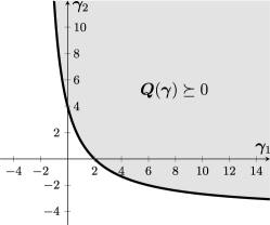
Figure 1: The shaded region indicates the feasible set of the LMI (23), given by the points $\bm{\gamma}=(\bm{\gamma}_{1},\bm{\gamma}_{2})$ satisfying both inequalities in (24). The thick black line indicates the boundary of the feasible set, given by the curve $\bm{\gamma}_{2}=(8-4\bm{\gamma}_{1})/(2+\bm{\gamma}_{1})$.

An optimization problem with a linear objective function subject to linear equalities and LMIs, i.e. in the form

$$\begin{gathered}\min_{\bm{\gamma}}\quad\bm{c}^{T}\bm{\gamma}\\ \begin{aligned} \text{s.t.}\quad\bm{A}\bm{\gamma}+\bm{b}&=0,\\ \bm{Q}(\bm{\gamma})&\succeq 0,\end{aligned}\end{gathered}$$ (25)

where $\bm{c}\in\mathbb{R}^{q}$ is the cost vector, $\bm{A}\in\mathbb{R}^{p\times q}$ and $\bm{b}\in\mathbb{R}^{p}$ define $p$ equality constraints and $\bm{Q}(\bm{\gamma})$ is as in (22), is known as a semidefinite program (SDP). Note that linear inequalities can be seen as one dimensional LMIs, and that multiple LMIs can always be combined into a single LMI Boyd et al. (1994); Boyd and Vandenberghe (2004), so the above form is general.

SDPs can be solved efficiently using well-established algorithms Boyd et al. (1994); Vandenberghe and Boyd (1996); Boyd and Vandenberghe (2004). Consequently, our strategy is to exploit the close relationship between the spectral constraint (11) and LMIs, and rewrite the variational problem for the minimization of $\mathcal{B}\{\phi\}$ as an SDP. To this end, we will parametrize the background field $\phi$ using a finite set of parameters (corresponding to the optimization variable $\bm{\gamma}$ in the above generic SDP), and enforce each functional inequality $\mathcal{Q}_{mn}\geq 0$ using sufficient conditions in the form of LMIs. This follows and extends the ideas already proposed by the authors in Fantuzzi and Wynn (2015a).

IV Bounds for the two dimensional flow

The bounding problem for the two dimensional flow is obtained from Sections II.2–II.3 by neglecting the $y$ direction. We will also drop the suffix $n$ from all variables and functionals for simplicity.

Equations (14)–(15) imply that $W_{0}=0$, so $\mathcal{Q}_{0}\geq 0$ for any choice of $\phi$. When $m\neq 0$, instead, we can use the incompressibility condition (14) to rewrite $U_{m}$ in terms of $W_{m}$ and hence express each $\mathcal{Q}_{m}$ as

$$\mathcal{Q}_{m}=\int\limits_{-1}^{1} \left[\frac{16}{\alpha_{m}^{2}}\left|\frac{d^{2}W_{m}}{d\zeta^{2}}\right|^{2}+8\left|\frac{dW_{m}}{d\zeta}\right|^{2}+\alpha_{m}^{2}\left|W_{m}\right|^{2}\right.$$

$$\left.-\frac{8}{\alpha_{m}}\frac{d\phi}{d\zeta}\,\text{\rm Im}\left(\frac{dW_{m}}{d\zeta}W_{m}^{*}\right)\right]d\zeta,$$ (26)

where the complex Fourier amplitudes $W_{m}(\zeta)$ satisfy the BCs

$$W_{m}(-1)=W_{m}(1)=\frac{dW_{m}}{d\zeta}\Big{|}_{-1}=\frac{d^{2}W_{m}}{d\zeta^{2}}\Big{|}_{1}=0.$$ (27)

The requirement that the Fourier modes combine into a real-valued velocity perturbation means that $\mathcal{Q}_{-m}=\mathcal{Q}_{m}$, so we can restrict the attention to positive $m$’s. Moreover, (20) guarantees that for a given choice of background field it suffices to consider $m$ up to the critical value

$$m_{c}(\phi):=\left\lfloor\frac{\Gamma_{x}}{\pi}\sqrt{\frac{1}{2}\left\|\frac{d\phi}{d\zeta}\right\|_{\infty}}\right\rfloor,$$ (28)

where $\lfloor\cdot\rfloor$ denotes the integer part of the argument.

After rescaling the BCs for $\phi$ in (10), the optimal bounds on $C_{\varepsilon}$ are determined by the solution of the variational problem

$$\min_{\phi}\quad\mathcal{B}\{\phi\}$$ (29)

s.t. $$\mathcal{Q}_{m}\{W_{m},\phi\}\geq 0 1\leq m\leq m_{c}(\phi),$$ ,

$$\phi(-1)=0$$ ,

$$\frac{d\phi}{d\zeta}\Big{|}_{1}=\frac{Gr}{2}$$ .

IV.1 Parametrization of the background field

The first step to rewrite (29) as an SDP is to parametrize the background field in terms of a finite number of decision variables. While the optimal $\phi$ cannot generally be described exactly with a finite dimensional parametrization, it can be approximated arbitrarily accurately by a polynomial of sufficiently high degree. Consequently, we restrict our attention to the family of background fields which are polynomials of degree at most $P+1$.

Since our analysis of the spectral constraints will be based on Legendre series expansions, we parametrize the background field by expressing its first derivative as

$$\frac{d\phi}{d\zeta}=\sum_{p=0}^{P}\hat{\phi}_{p}\,\mathcal{L}_{p}(\zeta),$$ (30)

where $\mathcal{L}_{p}(\zeta)$ is the Legendre polynomial of degree $p$.

The vector of Legendre coefficients $\bm{\hat{\phi}}=(\hat{\phi}_{0},...,\hat{\phi}_{P})^{T}$ must be chosen so as to impose the correct BCs on $\phi$. The condition $\phi(-1)=0$ can always be enforced by an appropriate choice of integration constant, while since $\mathcal{L}_{p}(1)=1$ Agarwal and O’Regan (2009) the condition at $\zeta=1$ becomes

$$\sum_{p=0}^{P}\hat{\phi}_{p}=\bm{1}^{T}\bm{\hat{\phi}}=\frac{\textit{Gr}}{2},$$ (31)

where $\bm{1}\in\mathbb{R}^{P+1}$ is a column vector of ones.

Finally, since $\left\|\mathcal{L}_{p}\right\|_{\infty}=1$ for all $p$ we have the useful estimate

$$\left\|\frac{d\phi}{d\zeta}\right\|_{\infty}=\max_{\zeta\in[-1,1]}\left|\sum_{p=0}^{P}\hat{\phi}_{p}\mathcal{L}_{p}(\zeta)\right|\leq\|\bm{\hat{\phi}}\|_{1},$$ (32)

where $\left\|\cdot\right\|_{1}$ denotes the usual $l^{1}$ norm.

IV.2 Formulation of a linear cost function

In order to formulate (29) as a standard SDP, we need to replace the quadratic objective functional $\mathcal{B}$ by an equivalent linear cost function. The orthogonality of the Legendre polynomials allows us to rewrite

$$\int\limits_{-1}^{1}\left(\frac{d\phi}{d\zeta}\right)^{2}d\zeta=\bm{\hat{\phi}}^{T}\bm{B}\bm{\hat{\phi}},$$ (33)

where $\bm{B}\in\mathbb{R}^{(P+1)\times(P+1)}$ is defined as

$$\bm{B}_{rs}=\frac{2\delta_{rs}}{2r+1},\qquad 0\leq r,s\leq P$$ (34)

and $\delta_{rs}$ is the usual Kroenecher delta. Moreover, using the results of Appendix A we have $\phi(1)=\phi(-1)+2\hat{\phi}_{0}$. Applying the boundary condition $\phi(-1)=0$, the objective functional $\mathcal{B}$ becomes

$$\mathcal{B}\{\phi\}=\frac{2}{Gr}\bm{\hat{\phi}}^{T}\bm{B}\bm{\hat{\phi}}-4\hat{\phi}_{0}.$$ (35)

Using a standard trick of convex optimization, we introduce an additional decision variable $\eta$ (called a slack variable) and minimize

$$\mathcal{B}_{\text{lin}}(\bm{\hat{\phi}},\eta):=\frac{2}{Gr}\eta-4\hat{\phi}_{0}$$ (36)

instead of $\mathcal{B}$, subject to the additional constraint that $\eta\geq\bm{\hat{\phi}}^{T}\bm{B}\bm{\hat{\phi}}$. Since $\bm{B}$ is invertible and its inverse is positive definite, Schur’s complement condition Boyd and Vandenberghe (2004) guarantees that

$$\bm{S}(\bm{\hat{\phi}},\eta):=\begin{bmatrix}\bm{B}^{-1}&\bm{\hat{\phi}}\\ \bm{\hat{\phi}}^{T}&\eta\end{bmatrix}\succeq 0\quad\Longleftrightarrow\quad\eta\geq\bm{\hat{\phi}}^{T}\bm{B}\bm{\hat{\phi}}.$$ (37)

Hence, the additional inequality constraint can be expressed as the LMI $\bm{S}(\bm{\hat{\phi}},\eta)\succeq 0$.

IV.3 Rigorous finite dimensional relaxation of $\mathcal{Q}_{m}$ using Legendre expansions

We now turn to the core problem of deriving a rigorous matrix representation for each of the constraints $\mathcal{Q}_{m}\geq 0$, which will allow us to enforce the spectral constraint using LMIs. As in Fantuzzi and Wynn (2015a), the analysis is based on the application of orthogonal series expansions. The need to enforce BCs other than periodicity prevents us from using the conventional Fourier series. As our analysis relies on $L^{2}$ orthogonality of the basis functions, we will use Legendre series expansions Jackson (1930); Zeidler (1995) (note that despite their attractive numerical properties, the more commonly used Chebyshev polynomials do not suit our purposes because they are only orthogonal with respect to the weight $\sqrt{1-\zeta^{2}}$). Some key results on Legendre expansions are reported in Appendix A. The details of the following analysis are quite technical, and will be omitted to keep the focus on our main objective — formulating an SDP whose solution gives a feasible background field for (29). LMI relaxations of integral inequalities using Legendre series will be thoroughly discussed in a future publication Fantuzzi and Wynn (2015b). Moreover, for notational neatness, we will drop the suffix $m$ from $\mathcal{Q}_{m}$, $W_{m}$ and $\alpha_{m}$; it should be understood that the following analysis holds for each individual $m\geq 1$.

Since the function $W$ represents the amplitude of a Fourier mode of a velocity perturbation, we assume it has enough regularity such that $W$, $\frac{dW}{d\zeta}$ and $\frac{d^{2}W}{d\zeta^{2}}$ can be expanded with the uniformly convergent Legendre series Jackson (1930); Zeidler (1995)

$$W =\sum_{n=0}^{\infty}\hat{w}_{n}\mathcal{L}_{n}(\zeta),$$ (38a)

$$\frac{dW}{d\zeta} =\sum_{n=0}^{\infty}\hat{w}^{\prime}_{n}\mathcal{L}_{n}(\zeta),$$ (38b)

$$\frac{d^{2}W}{d\zeta^{2}} =\sum_{n=0}^{\infty}\hat{w}^{\prime\prime}_{n}\mathcal{L}_{n}(\zeta).$$ (38c)

Since $W$ is complex valued, so are the Legendre coefficients $\hat{w}_{n}$, $\hat{w}_{n}^{\prime}$ and $\hat{w}_{n}^{\prime\prime}$. In addition, the results of Appendix A and the BCs at $\zeta=-1$ from (27) imply that the Legendre coefficients are related by the compatibility conditions

$$\hat{w}_{0} =\hat{w}^{\prime}_{0}-\frac{\hat{w}^{\prime}_{1}}{3},$$ (39a)

$$\hat{w}_{n} =\frac{\hat{w}^{\prime}_{n-1}}{2n-1}-\frac{\hat{w}^{\prime}_{n+1}}{2n+3},\qquad n\geq 1,$$

and

$$\hat{w}^{\prime}_{0} =\hat{w}^{\prime\prime}_{0}-\frac{\hat{w}^{\prime\prime}_{1}}{3},$$ (39b)

$$\hat{w}^{\prime}_{n} =\frac{\hat{w}^{\prime\prime}_{n-1}}{2n-1}-\frac{\hat{w}^{\prime\prime}_{n+1}}{2n+3},\qquad n\geq 1.$$

Rather than truncating the Legendre series of $W$ after $N$ terms to obtain an approximation of $\mathcal{Q}$, we consider the full infinite dimensional quadratic form by defining the remainder functions

$$\tilde{w}_{0}(\zeta) :=\sum_{n=N+1}^{\infty}\hat{w}_{n}\mathcal{L}_{n}(\zeta),$$ (40a)

$$\tilde{w}_{1}(\zeta) :=\sum_{n=N+2}^{\infty}\hat{w}^{\prime}_{n}\mathcal{L}_{n}(\zeta),$$ (40b)

$$\tilde{w}_{2}(\zeta) :=\sum_{n=N+P+4}^{\infty}\hat{w}^{\prime\prime}_{n}\mathcal{L}_{n}(\zeta).$$ (40c)

The lower limit in (40b) is motivated by (39a), while the lower limit $N+P+4$ in (40c) is chosen for convenience; this will become apparent in Appendix B.

In Appendix B, we show that there exist a real, symmetric, positive definite matrix $\bm{Q}_{1}\in\mathbb{R}^{(N+P+4)\times(N+P+4)}$, and a real (but not symmetric) matrix $\bm{Q}_{2}(\bm{\hat{\phi}})\in\mathbb{R}^{(N+P+4)\times(N+P+4)}$, whose entries are linear in $\bm{\hat{\phi}}$, such that

$$\mathcal{Q}\{W,\phi\}= \left(\bm{\hat{w}}^{\prime\prime}\right)^{\dagger}\bm{Q}_{1}\bm{\hat{w}}^{\prime\prime}-\text{\rm Im}\left[\left(\bm{\hat{w}}^{\prime\prime}\right)^{\dagger}\bm{Q}_{2}(\bm{\hat{\phi}})\bm{\hat{w}}^{\prime\prime}\right]$$

$$+\mathcal{R}\{\tilde{w}_{0},\tilde{w}_{1},\tilde{w}_{2},\phi\}.$$ (41)

Here, $(\cdot)^{\dagger}$ denotes conjugate transposition, $\bm{\hat{w}}^{\prime\prime}\in\mathbb{C}^{N+P+4}$ is the column vector containing the Legendre coefficients $\hat{w}^{\prime\prime}_{0}$, …, $\hat{w}^{\prime\prime}_{N+P+3}$ and

$$\mathcal{R}\{\tilde{w}_{0},\tilde{w}_{1},\tilde{w}_{2},\phi\}:=\int\limits_{-1}^{1} \left[\frac{16}{\alpha^{2}}\left|\tilde{w}_{2}\right|^{2}+8\left|\tilde{w}_{1}\right|^{2}+\alpha^{2}\left|\tilde{w}_{0}\right|^{2}\right.$$

$$\left.-\frac{8}{\alpha}\frac{d\phi}{d\zeta}\,\text{\rm Im}\left(\tilde{w}_{1}\tilde{w}_{0}^{*}\right)\right]d\zeta.$$ (42)

We also show in Appendix C that

$$\mathcal{R}\{\tilde{w}_{0},\tilde{w}_{1},\tilde{w}_{2},\phi\}\geq -\|\bm{\hat{\phi}}\|_{1}\left(\bm{\hat{w}}^{\prime\prime}\right)^{\dagger}\bm{R}\bm{\hat{w}}^{\prime\prime}$$

$$+\frac{16}{\alpha^{2}}\left(1-\kappa\|\bm{\hat{\phi}}\|_{1}\right)\left\|\tilde{w}_{2}\right\|^{2}_{2},$$ (43)

where $\left\|\cdot\right\|_{2}$ is the usual $L^{2}$ norm, $\bm{R}\in\mathbb{R}^{(N+P+4)\times(N+P+4)}$ is a positive definite real matrix whose Frobenius norm $\left\|\bm{R}\right\|_{F}$ scales as $\mathcal{O}(N^{-4})$, and $\kappa$ is a positive constant scaling as $\mathcal{O}(N^{-3})$ (see Figure 2). A more in-depth discussion of the properties of $\bm{Q}_{1}$, $\bm{Q}_{2}$, $\bm{R}$ and $\kappa$ will be given elsewhere Fantuzzi and Wynn (2015b).

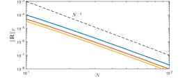
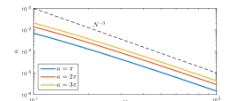
Figure 2: (Color Online) Decay of the Frobenius norm of the matrix $\bm{R}$ (top) and the constant $\kappa$ (bottom) for selected wavenumbers $\alpha$.

Considering the real and imaginary parts of $\bm{\hat{w}}^{\prime\prime}$ explicitly and defining

$$\bm{M}(\bm{\hat{\phi}}):=\mathrm{sym}\left(\begin{bmatrix}\displaystyle\bm{Q}_{1}-\|\bm{\hat{\phi}}\|_{1}\bm{R}&-\bm{Q}_{2}(\bm{\hat{\phi}})\\ \bm{Q}_{2}(\bm{\hat{\phi}})&\displaystyle\bm{Q}_{1}-\|\bm{\hat{\phi}}\|_{1}\bm{R}\end{bmatrix}\right),$$ (44)

where $\mathrm{sym}(\cdot)$ denotes the symmetric part of a matrix, we obtain the rigorous lower bound

$$\mathcal{Q}\{W,\phi\}\geq\Psi\{\bm{\hat{w}}^{\prime\prime},\tilde{w}_{2},\phi\},$$ (45)

where

$$\Psi\{\bm{\hat{w}}^{\prime\prime},\tilde{w}_{2},\phi\}:= \begin{bmatrix}\text{\rm Re}\left(\bm{\hat{w}}^{\prime\prime}\right)\\ \text{\rm Im}\left(\bm{\hat{w}}^{\prime\prime}\right)\end{bmatrix}^{T}\bm{M}(\bm{\hat{\phi}})\begin{bmatrix}\text{\rm Re}\left(\bm{\hat{w}}^{\prime\prime}\right)\\ \text{\rm Im}\left(\bm{\hat{w}}^{\prime\prime}\right)\end{bmatrix}$$

$$+\frac{16}{\alpha^{2}}\left(1-\kappa\,\|\bm{\hat{\phi}}\|_{1}\right)\left\|\tilde{w}_{2}\right\|^{2}_{2}.$$ (46)

Note that this lower bound holds for all functions $W$ that satisfy the BCs at $\zeta=-1$ in (27). Consequently, the positivity of $\mathcal{Q}$ is proven for any $W$ satisfying the boundary conditions at $\zeta=-1$ if we enforce

$$\bm{M}(\bm{\hat{\phi}})\succeq 0,$$ (47a)

$$1-\kappa\|\bm{\hat{\phi}}\|_{1}\geq 0.$$ (47b)

However, $\mathcal{Q}$ needs only be positive for any $W$ satisfying all BCs in (27), which is a weaker statement. Recalling that $\mathcal{L}_{p}(\pm 1)=(\pm 1)^{p}$ for all $p$, with the help of (39) and letting $\bm{1}\in\mathbb{R}^{N+P+4}$ be a column vector of ones, the BCs at $\zeta=1$ from (27) can be expressed as

$$\hat{w}^{\prime\prime}_{0}-\frac{\hat{w}^{\prime\prime}_{1}}{3}=0,$$ (48a)

$$\bm{1}^{T}\bm{\hat{w}}^{\prime\prime}+\tilde{w}_{2}(1)=0.$$ (48b)

The first of these conditions can be imposed by letting

$$\bm{\hat{w}}^{\prime\prime}=\bm{A}\bm{\hat{\omega}},$$ (49)

where

$$\bm{\hat{\omega}}:=\begin{pmatrix}\hat{w}^{\prime\prime}_{1}\\ \vdots\\ \hat{w}^{\prime\prime}_{N+P+3}\end{pmatrix},\qquad\bm{A}:=\begin{bmatrix}{}^{1}/_{3}&0&\ldots&0\\ 1&0&\ldots&0\\ 0&1&\ldots&0\\ \vdots&&\ddots&\vdots\\ 0&\ldots&0&1\end{bmatrix}.$$

Substituting this representation in (IV.3) and defining

$$\bm{Q}(\bm{\hat{\phi}}):=\begin{bmatrix}\bm{A}&\bm{0}\\ \bm{0}&\bm{A}\end{bmatrix}^{T}\bm{M}(\bm{\hat{\phi}})\begin{bmatrix}\bm{A}&\bm{0}\\ \bm{0}&\bm{A}\end{bmatrix}$$ (50)

we obtain

$$\Psi\{\bm{\hat{w}}^{\prime\prime},\tilde{w}_{2},\phi\}= \begin{bmatrix}\text{\rm Re}\left(\bm{\hat{\omega}}\right)\\ \text{\rm Im}\left(\bm{\hat{\omega}}\right)\end{bmatrix}^{T}\bm{Q}(\bm{\hat{\phi}})\begin{bmatrix}\text{\rm Re}\left(\bm{\hat{\omega}}\right)\\ \text{\rm Im}\left(\bm{\hat{\omega}}\right)\end{bmatrix}$$

$$+\frac{16}{\alpha^{2}}\left(1-\kappa\,\|\bm{\hat{\phi}}\|_{1}\right)\left\|\tilde{w}_{2}\right\|^{2}_{2}.$$ (51)

Thus, the spectral constraint can be enforced via the sufficient finite dimensional conditions

$$\bm{Q}(\bm{\hat{\phi}})\succeq 0,$$ (52a)

$$1-\kappa\,\|\bm{\hat{\phi}}\|_{1}\geq 0,$$ (52b)

which are weaker than (47) and, consequently, allow us to compute a better bound.

These sufficient conditions could be weakened further if (48b) could be incorporated. However, this is difficult to achieve since $\tilde{w}_{2}(1)$ does not appear explicitly in (IV.3). Moreover, we show in Appendix D that (52) must still be satisfied if $\Psi\geq 0$ when (48b) holds. Consequently, we choose to enforce the spectral constraint via (52).

Remark 1

Since the matrix $\bm{R}$ of equation (IV.3) gives a negative definite contribution to $\bm{Q}$ and $\kappa$ is positive, it is not obvious that the conditions in (52) are feasible. However, $\left\|\bm{R}\right\|_{F}$ and $\kappa$ decay to zero as at least as fast as $N^{-3}$. Under the reasonable assumption that a strictly feasible polynomial background field of degree $P+1$ exists for (11), we expect that a vector $\bm{\hat{\phi}}$ satisfying (52) exists when $N$ is sufficiently large. Moreover, although the size of $\bm{Q}$ increases linearly with $N$, the fast decay of $\left\|\bm{R}\right\|_{F}$ and $\kappa$ means that in practice the required $N$ is small enough that (52a) is a numerically tractable constraint.

Remark 2

Conditions (52) need to be derived and imposed for a range of wavenumbers $\alpha_{m}$, $m=1,...,m_{c}$. Since $\kappa$ increases linearly with $\alpha_{m}$ (equivalently, with $m$, cf. Appendix C), we expect that the truncation $N$ required to make (52b) feasible increases with $m$. Similarly, although $\left\|\bm{R}\right\|_{F}$ decreases linearly with $m$ (cf. Appendix C), the dominant positive definite contribution to $\bm{Q}(\bm{\hat{\phi}})$ — which comes from the the second derivative term in the functional $\mathcal{Q}$ — decays as $m^{-2}$. Hence, we again expect that a higher truncation $N$ will be required to make (52a) feasible for large values of $m$.

IV.4 An SDP for the optimal bounds

The conditions in (52) are not LMIs due to the appearance of absolute values in $\|\bm{\hat{\phi}}\|_{1}$, but can be recast as LMIs by introducing a vector $\bm{t}=(t_{0},...,t_{P})^{T}$ of slack variables, replacing $\|\bm{\hat{\phi}}\|_{1}$ with $\bm{1}^{T}\bm{t}=\sum_{p=0}^{P}t_{p}$ and introducing $2P+2$ inequality constraints of the form

$$\hat{\phi}_{j}-t_{j}\leq 0,\qquad\hat{\phi}_{j}+t_{j}\geq 0.$$ (53)

As a result, each of the functional inequalities $\mathcal{Q}_{m}\geq 0$ in (29) can be replaced by the LMI $\bm{Q}_{m}(\bm{\hat{\phi}},\bm{t})\succeq 0$ and the linear inequality $1-\kappa_{m}\bm{1}^{T}\bm{t}\geq 0$ (where $\bm{Q}_{m}$ and $\kappa_{m}$ are derived as in Section IV.3 for each $m$). Together with equations (36)–(37), this means that bounds on $C_{\varepsilon}$ can be computed at each Gr after solving the SDP

$$\min_{\eta,\bm{\hat{\phi}},\bm{t}}\qquad\frac{2}{Gr}\eta-4\hat{\phi}_{0}$$ (54)

$$\begin{aligned} \text{s.t.}\qquad\qquad\bm{S}(\bm{\hat{\phi}},\eta)\succeq 0,&\\ \bm{Q}_{m}(\bm{\hat{\phi}},\bm{t})\succeq 0,&&&&&1\leq m\leq m_{c},\\ 1-\kappa_{m}\bm{1}^{T}\bm{t}\geq 0,&&&&&1\leq m\leq m_{c},\\ \hat{\phi}_{j}-t_{j}\leq 0,&&&&&0\leq j\leq P,\\ \hat{\phi}_{j}+t_{j}\geq 0,&&&&&0\leq j\leq P,\\ \bm{1}^{T}\bm{\hat{\phi}}=\frac{\textit{Gr}}{2}.\end{aligned}$$

Strictly speaking, the bounds computed with the solution of this SDP are not optimal, but only near-optimal because they are obtained using a restricted class of background fields and imposing a stronger condition than the original spectral constraint. In practice, however, we can increase the parameters $N$ and $P$ until the solution of the SDP has converged to that of (29) — at the expense of increasing the computational cost of the optimization.

In addition, the analysis of Section IV.3 guarantees that the background field constructed with the optimal $\bm{\hat{\phi}}$ is a feasible choice for (29), so the bounds computed at each Gr would be rigorous if the numerical roundoff errors in the solution of (54) were tracked and carefully taken into account. The implementation of algorithms to solve (54) rigorously is beyond the scope of this work and the bounds presented in the following sections cannot be considered analytical results. However, a fully computer-assisted proof of near-optimal bounds does not seem beyond the reach of future work.

Finally, we remark that $m_{c}$ depends on $\phi$ according to (28), so the number of inequalities in the SDP is not known a priori. This means that an iterative procedure is needed: solve the optimization using a suitable initial guess $m_{0}$ for $m_{c}$, calculate the correct $m_{c}$ with (28) after the optimization, and check the full set of LMIs a posteriori; if any constraints are violated, the optimization is repeated with the updated $m_{c}$. We also remark that the role of $m_{c}$ is that of an upper bound on the largest critical Fourier mode — that is the largest value of $m$ for which the constraints in (54) are active. Of course, if one knew the exact critical modes a priori, one could solve the SDP by considering only such modes. However, the fact that the number of inequalities in (54) is unknown is not due to the lack of knowledge of the exact critical modes, but only to the dependence of $m_{c}$ on $\phi$. In fact, if one could find an explicit value for $m_{c}$, say in terms of the Grashoff number, the number of LMIs in the SDP would be well defined and no iterative procedure would be required.

IV.5 Numerical implementation and results

Table 1: Problem data, memory requirements and CPU time for selected SDP instances. CPU time and memory include pre- and post-processing routines as well as the solution of the SDP.

$\Gamma_{x}$	Gr	$m_{0}$	$P$	$N$	RAM (Mb)	Time (s)	$m_{c}$	$N_{\mathrm{checks}}$
2	$10^{3}$	5	19	100	7.4	50	12	100
2	$10^{4}$	8	29	125	25.3	160	38	125
2	$10^{5}$	15	34	150	71.7	1280	116	350
3	$10^{3}$	5	19	100	7.3	59	18	100
3	$10^{4}$	10	29	125	31.6	188	57	125
3	$10^{5}$	25	34	150	119.4	2608	174	350

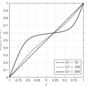
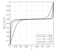
Figure 3: Background fields normalized by their value at $\zeta=1$ for selected Grashoff numbers and $\Gamma_{x}=2$.

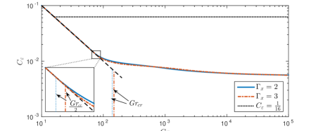
Figure 4: (Color Online) Optimal upper bounds on $C_{\varepsilon}$ for $\Gamma_{x}=2$ and $\Gamma_{x}=3$, compared to the analytical bound $C_{\varepsilon}\leq\frac{1}{16}$ from Hagstrom and Doering (2014). The laminar dissipation coefficient is shown as a dashed black line. Detail: as expected, the bounds depart from the laminar $C_{\varepsilon}$ at $\textit{Gr}=0.5\textit{Gr}_{\text{cr}}$, where $\textit{Gr}_{\text{cr}}=139.54$ for $\Gamma_{x}=2$ and $Gr_{cr}=148.66$ for $\Gamma_{x}=3$ (also shown).

The SDP (54) was solved in MATLAB using the optimization toolbox YALMIP Löfberg (2004) and the SDP solver SeDuMi Sturm (1999) for $10\leq\textit{Gr}\leq 10^{5}$ and for two values of domain aspect ratio, $\Gamma_{x}=2$ and $\Gamma_{x}=3$. All computations were carried out on a desktop computer with an Intel Core i7 3.40GHz CPU and 16Gb of RAM. At each Gr, we chose an initial guess $m_{0}$, fixed the degree $P$ of the background field and the number $N$ of Legendre modes of the perturbations, and solved the SDP. We increased $P$ and $N$ until the optimal bounds on $C_{\varepsilon}$ changed by less than approximately $1$%. Finally, given the optimal background field, we computed $m_{c}(\phi)$ with (28) and verified that $\phi$ was feasible for all $m\leq m_{c}$. Since in practice $m_{c}\gg m_{0}$ at large Gr, we expect that these checks might fail for the largest values of $m$ (cf. Remark 2). Before repeating the optimization with the updated set of LMIs, we therefore try to validate the background field with an increased value of $N$. In the following, we will refer to this value as $N_{\mathrm{checks}}$.

Details of the problem specifications, memory requirements, computation time and a posteriori checks for selected SDP instances are reported in Table 1. The reason for the disparity in the number of Legendre coefficients used for the background field and the perturbation is that $N$ needs to be large to make the negative definite terms in the constraints small enough to obtain a feasible and accurate SDP formulation of (29) (cf. Remark 1). Instead, the optimal $\phi$ is well resolved with modest $P$.

Figure 3 shows some of the optimal background fields obtained for $\Gamma_{x}=2$, normalized by their boundary value $\phi(1)$. Analogous results were obtained for $\Gamma_{x}=3$ and are not shown for brevity. As Gr is raised, the background fields evolve from the linear Couette profile, developing two boundary layers in a similar way to that observed by Nicodemus et al. Nicodemus et al. (1997) for the classical Couette flow. The asymmetric depth of the boundary layers reflects the asymmetry of the BCs.

The bounds on $C_{\varepsilon}$ corresponding to the optimal background fields are illustrated in Figure 4, along with the laminar dissipation coefficient and the analytical bound $C_{\varepsilon}\leq 1/16=0.0625$ proven in Hagstrom and Doering (2014). Although energy stability analysis indicates that the laminar Couette flow is stable up to the critical Grashoff number $\textit{Gr}_{\text{cr}}=139.54$ for $\Gamma_{x}=2$ and $\textit{Gr}_{\text{cr}}=148.66$ for $\Gamma_{x}=3$ (cf. Section VI), our bounds deviate from the laminar value $C_{\varepsilon}=\textit{Gr}^{-1}$ when $\textit{Gr}\geq 0.5\textit{Gr}_{\text{cr}}$. This was expected, because the spectral constraint of the bounding problem differs from that of the energy stability problem by a factor of 2 when letting $\phi=\bm{u}_{L}$ (cf. equations (6) and (11) in Section II). While this limitation could be overcome by the addition of a balance parameter in the spectral constraint (see e.g. Nicodemus et al. (1998a); Wittenberg and Gao (2010); Wen et al. (2015)), it allows us to check that the solution of our SDP has converged to that of the original bounding problem.

As predicted by the analytical bounds of Hagstrom and Doering (2014), the results suggest that $C_{\varepsilon}$ approaches a constant when $\textit{Gr}\to\infty$ independently of $\Gamma_{x}$, meaning that the dissipation coefficient becomes independent of the flow viscosity and aspect ratio. The quantitative improvement, however, is evident: our near-optimal bound is more than 10 times smaller than the analytical result at $\textit{Gr}=10^{5}$. Unfortunately, the limited range of Gr does not allow us to confidently estimate an asymptotic value for $C_{\varepsilon}$ (see Section IV.6 for further comments on the computational issues at large Gr). Moreover, we could not compare our bounds to values of $C_{\varepsilon}$ extracted from experiments or direct numerical simulations because, to the best of our knowledge, such data are not available. Although it is unlikely that there exists a solution to the Navier–Stokes equation whose associated dissipation coefficient equals our bounds Tang et al. (2004), performing this comparison remains in the interest of future research.

The slight oscillations in the numerical bounds for $10^{2}\lesssim\textit{Gr}\lesssim 10^{4}$ are due to the occurrence of bifurcations in the number of critical Fourier modes, that is the number of values $m$ such that the minimum of $\mathcal{Q}_{m}$ over non trivial functions is zero. This minimum coincides with the ground state eigenvalue $\lambda_{0}$ of the linear operator associated with $\mathcal{Q}_{m}$, and corresponds to the minimum eigenvalue of the matrix $\bm{Q}_{m}$, rescaled so that the respective eigenvector defines an eigenfunction $W_{m}$ with unit $L^{2}$ norm. Some selected values of $\lambda_{0}$ computed for $\textit{Gr}=10^{4}$ are plotted in Figure 5, while the critical ground state eigenfunctions are shown in Figure 6. Note that although conditions (52) do not enforce (48b) explicitly, the critical modes satisfy all the correct BCs.

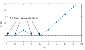
Figure 5: (Color Online) Selected ground-state eigenvalues $\lambda_{0}$ of the linear operators generating the quadratic form $\mathcal{Q}_{m}$ at $\textit{Gr}=10^{4}$. The values of $\lambda_{0}$ correspond to the minimum of $\mathcal{Q}_{m}$ subject to the unit–norm constraint $\left\|W_{m}\right\|^{2}_{2}=1$.

Figure 6: (Color Online) Real part (solid line) and imaginary part (dot-dashed line) of the critical ground state eigenfunctions and their derivatives at $\textit{Gr}=10^{4}$, normalized so that $\left\|W_{m}\right\|^{2}_{2}=1$.

IV.6 Computational issues

As already mentioned, the range of Grashoff numbers we could study does not stretch into the expected asymptotic regime. This (current) limitation is a drawback of our method, as one would hope to be able to extract accurate scaling laws for large values of Gr.

A first limiting factor is that although the memory requirements for our largest SDP are modest and the computation times reasonable, we observed that the solution of the SDP became less accurate and prone to numerical ill conditioning as we increased Gr (and, consequently, the values of $P$, $N$ and $m_{0}$). We expect that careful rescaling of the SDP data might help to resolve this issue; yet, a general procedure is not available, and we leave the development of an appropriate rescaling strategy to future work.

A second known issue is that the algorithms implemented in general purpose SDP solvers such as SeDuMi do not scale well with increasing problem size (see e.g. Fukuda et al. (2000); Wen et al. (2010) for more details), and we expect that they will become unsuitable to solve the large SDPs needed at very large Grashoff numbers. Addressing the challenges posed by large SDPs is the subject of a very active field of research (see e.g. Fukuda et al. (2000); Nakata et al. (2003); Burer and Monteiro (2003, 2005); Burer and Choi (2006); Wen et al. (2010); Sun et al. (2014)). In particular, the used of dedicated algorithms instead of general purpose SDP solvers should be considered in future investigations, but is beyond the scope of the present work.

Finally, the task of validating the solution returned by the SDP solver might pose a challenge of its own if memory requirements and computation time are a constraint. This is due to the cost of performing a large number of eigenvalue computations to check that the (generally large) matrices $\bm{Q}_{m}(\bm{\hat{\phi}},\bm{t})$ are positive semidefinite for all $m$’s up to the correct $m_{c}$. For example, at $\textit{Gr}=10^{5}$ and with $P=34$, $N_{\mathrm{checks}}=350$, we had to compute the eigenvalues of a $774\times 774$ matrix 116 times for $\Gamma_{x}=2$ and 174 times for $\Gamma_{x}=3$ (cf. Table 1); in these cases, validating the solution was the most time-consuming task of the entire computation. In this case, a more careful estimate for $m_{c}$ might be helpful.

V Bounds for the three dimensional flow

To study the three dimensional flow, we follow Tang et al. (2004); Hagstrom and Doering (2014) and make the reasonable (although unproven) assumption that the critical modes determining the background field are independent of $x$ and, consequently, of the aspect ratio in the $x$ direction $\Gamma_{x}$. This assumption is not necessary for our method, but it simplifies the following analysis. Moreover, and most importantly, it reduces the size of the SDP we need to solve, as well as the cost of our a posteriori checks. This allows us to consider a wider range of Gr at a reasonable computational cost, and therefore to draw relevant conclusions regarding the flow properties.

After setting $\alpha_{m}=0$ in Section II.3 and dropping the suffix $m$ to simplify the notation, the incompressibility condition allows us to eliminate $V_{n}$ and rewrite the quadratic forms $\mathcal{Q}_{n}$ as

$$\mathcal{Q}_{n}=\int\limits_{-1}^{1} \left[\beta_{n}^{2}\left|U_{n}\right|^{2}+4\left|\frac{dU_{n}}{d\zeta}\right|^{2}+\beta_{n}^{2}\left|W_{n}^{2}\right|+8\left|\frac{dW_{n}}{d\zeta}\right|^{2}\right.$$

$$\left.+\frac{16}{\beta_{n}^{2}}\left|\frac{d^{2}W_{n}}{d\zeta^{2}}\right|^{2}+4\frac{d\phi}{d\zeta}\text{\rm Re}\left(U_{n}W_{n}^{*}\right)\right]d\zeta,$$ (55)

where the complex functions $U_{n}$ and $W_{n}$ satisfy the homogeneous BCs

$$U_{n}(-1)=\frac{dU_{n}}{d\zeta}\Big{|}_{1}=0,$$ (56a)

$$W_{n}(-1)=W_{n}(1)=\frac{dW_{n}}{d\zeta}\Big{|}_{-1}=\frac{d^{2}W_{n}}{d\zeta^{2}}\Big{|}_{1}=0.$$ (56b)

Since the real and imaginary parts of $U_{n}$ and $W_{n}$ give independent and formally identical contributions to $\mathcal{Q}_{n}$, to show that $\mathcal{Q}_{n}\geq 0$ it suffices to assume that $U_{n}$ and $W_{n}$ are real functions. Moreover, as in the two dimensional case, it is enough to consider strictly positive $n$’s up to the critical value

$$n_{c}(\phi):=\left\lfloor\frac{\Gamma_{y}}{\pi}\sqrt{\frac{1}{2}\left\|\frac{d\phi}{d\zeta}\right\|_{\infty}}\right\rfloor.$$ (57)

Consequently, the optimal bounds on $C_{\varepsilon}$ are determined by the solution of the variational problem

$$\min_{\phi}\quad\mathcal{B}\{\phi\}$$ (58)

s.t. $$\mathcal{Q}_{n}\{U_{n},W_{n},\phi\}\geq 0, 1\leq n\leq n_{c}(\phi),$$

$$\phi(-1)=0,$$

$$\frac{d\phi}{d\zeta}\Big{|}_{1}=\frac{Gr}{2}.$$

V.1 An SDP for the optimal bounds

As for the two dimensional flow, the variational problem (58) can be recast as an SDP. In particular, we can use the parametrization of the background field and the linear objective function of Sections IV.1–IV.2. Following analogous steps to Section IV.3, we can expand $U_{n}$ and $W_{n}$ with appropriate Legendre series, consider $N$ coefficients explicitly and show that

$$\mathcal{Q}_{n}\geq \,\,\bm{\hat{\omega}}^{T}\bm{Q}_{n}(\bm{\hat{\phi}})\bm{\hat{\omega}}+4\left(1-\kappa_{n}\|\bm{\hat{\phi}}\|_{1}\right)\left\|\tilde{u}_{1}\right\|_{2}^{2}$$

$$+\frac{16}{\beta_{n}^{2}}\left(1-\rho_{n}\|\bm{\hat{\phi}}\|_{1}\right)\left\|\tilde{w}_{2}\right\|_{2}^{2}.$$ (59)

Here, $\bm{\hat{\omega}}$ is a vector containing the Legendre coefficients of $\frac{dU_{n}}{d\zeta}$ and $\frac{d^{2}W_{n}}{d\zeta^{2}}$ after imposing the BCs, while $\tilde{u}_{1}$ and $\tilde{w}_{2}$ are the corresponding remainder functions. Moreover, $\bm{Q}_{n}$ is a real, symmetric matrix whose entries are affine in $\bm{\hat{\phi}}$ and $\|\bm{\hat{\phi}}\|_{1}$, while $\kappa_{n}$ and $\rho_{n}$ are positive constants that decay with $N$. The details are similar to those of Section IV.3, and are omitted for brevity; we refer the interested reader to the more general discussion of Fantuzzi and Wynn (2015b).

As in Section IV.4, we can introduce a vector of slack variables $\bm{t}$ and add the $2P+2$ constraints ${\hat{\phi}_{j}-t_{j}\leq 0}$, ${\hat{\phi}_{j}+t_{j}\geq 0}$ to remove any absolute values from the right-hand side of (V.1). We can then replace each functional inequality $\mathcal{Q}_{n}\geq 0$ with the LMI $\bm{Q}_{n}(\bm{\hat{\phi}},\bm{t})\succeq 0$ and two linear inequalities, and compute near-optimal bounds on $C_{\varepsilon}$ at each Gr after solving the SDP

$$\min_{\eta,\bm{\hat{\phi}},\bm{t}}\qquad\frac{2}{Gr}\eta-4\hat{\phi}_{0}$$ (60)

$$\begin{aligned} \text{s.t.}\qquad\qquad\bm{S}(\bm{\hat{\phi}},\eta)\succeq 0,&\\ \bm{Q}_{n}(\bm{\hat{\phi}},\bm{t})\succeq 0,&&&&&1\leq n\leq n_{c},\\ 1-\kappa_{n}\bm{1}^{T}\bm{t}\geq 0,&&&&&1\leq n\leq n_{c},\\ 1-\rho_{n}\bm{1}^{T}\bm{t}\geq 0,&&&&&1\leq n\leq n_{c},\\ \hat{\phi}_{j}-t_{j}\leq 0,&&&&&0\leq j\leq P,\\ \hat{\phi}_{j}+t_{j}\geq 0,&&&&&0\leq j\leq P,\\ \bm{1}^{T}\bm{\hat{\phi}}=\frac{\textit{Gr}}{2}.\end{aligned}$$

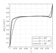
Figure 7: Background fields normalized by their value at $\zeta=1$ for selected Grashoff numbers and $\Gamma_{y}=3$.

As for the two dimensional case, we stress that the solution to this SDP gives a feasible background field for the infinite dimensional variational problem (58) (modulo roundoff errors due to finite precision arithmetic).

Finally, as in Section IV.4, the number of inequalities $n_{c}$ is not known a priori, so we will solve the optimization using an initial guess $n_{0}$, verify the full set of LMIs a posteriori as outlined in Section IV.5, and repeat the optimization with an updated $n_{c}$ if such checks fail.

V.2 Numerical implementation and results

Table 2: Problem data, memory requirements and CPU time for selected SDP instances. CPU time and memory include pre- and post-processing routines as well as the solution of the SDP.

$\Gamma_{y}$	Gr	$n_{0}$	$P$	$N$	RAM (Mb)	Time (s)	$n_{c}$	$N_{\mathrm{checks}}$
2	$10^{2}$	5	34	100	15.1	55	5	100
2	$10^{3}$	10	39	125	46.9	168	14	125
2	$10^{4}$	10	44	150	68.2	245	44	150
3	$10^{2}$	5	34	100	15.1	53	7	100
3	$10^{3}$	10	39	125	46.9	105	21	125
3	$10^{4}$	10	44	150	68.2	269	65	150

The SDP (60) was solved in MATLAB for $10\leq\textit{Gr}\leq 10^{4}$ and domain aspect ratios $\Gamma_{y}=2$, $\Gamma_{y}=3$. The problem specifications, memory requirements and computational time for selected values of Gr are shown in Table 2. Note that, compared to the two dimensional case, higher polynomial degrees were required at a given Gr to resolve the finer structures characterizing the optimal background fields. The details of the numerical implementation are as in Section IV.5, and as in Section IV.6 the loss of accuracy in the solution of the SDP prevented us from reliably increasing Gr to larger values.

A selection of optimal profiles for $\Gamma_{y}=3$ is shown in Figure 7 (analogous results were obtained for $\Gamma_{y}=2$). Interestingly, as Gr is raised the boundary layer near the top boundary ($\zeta=1$) overshoots the approximately constant value in the bulk of the domain, resulting in a non-monotonic layer. The boundary layer near $\zeta=-1$, instead, develops two regions with different characteristic slope (steeper near the boundary, flatter towards the edge). We observed that the structural change leading to this “internal layer” near $\zeta=-1$ corresponds to the occurrence of bifurcations in the number of critical Fourier modes in the SDP; Figure 8 shows that 3 bifurcations have occurred at $\textit{Gr}=10^{4}$. A similar behavior was also observed by Nicodemus et al. Nicodemus et al. (1997), who computed optimal background fields for the classical Couette flow, suggesting that the qualitative structural properties of the optimal background field at the bottom boundary are not affected by a change in the surface forcing.

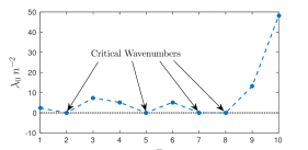
Figure 8: (Color Online) Selected ground state eigenvalues $\lambda_{0}$ of the linear operators generating the quadratic form $\mathcal{Q}_{n}$ at $\textit{Gr}=10^{4}$. The values of $\lambda_{0}$ correspond to the minimum of $\mathcal{Q}_{n}$ subject to the unit norm constraint $\left\|U_{n}\right\|^{2}_{2}+\left\|W_{n}\right\|^{2}_{2}=1$.

Figure 9: (Color Online) Optimal upper bounds on $C_{\varepsilon}$ for $\Gamma_{y}=2$ and $\Gamma_{y}=3$, compared to the numerical bounds from Tang et al. (2004) (valid at large Gr). The laminar dissipation coefficient is shown as a dashed black line, while the analytical bound $C_{\varepsilon}\lesssim 0.3536$ proven in Hagstrom and Doering (2014) is not plotted for clarity. Detail: as expected, our near-optimal bounds depart from the laminar value at $\textit{Gr}=0.5\textit{Gr}_{\text{cr}}$.

The optimal bounds are plotted in Figure 9, along with the laminar $C_{\varepsilon}$ and the asymptotic bounds estimated by Tang et al. — accurate for $\textit{Gr}\gtrsim 500$ (Tang et al., 2004, Figure 3(b)). As for the two dimensional case, the bounds deviate from the laminar value at the expected value $\textit{Gr}=0.5\textit{Gr}_{\text{cr}}$, where $\textit{Gr}_{\text{cr}}=57.20$ for $\Gamma_{y}=2$ and $\textit{Gr}_{\text{cr}}=51.73$ for $\Gamma_{y}=3$ (cf. Section VI). This confirms that the solution of the SDP has converged to the optimal solution of (58).

The quantitative improvement compared to the analytical bound $C_{\varepsilon}\leq{1}/{(2\sqrt{2})}\approx 0.3536$ proven in Hagstrom and Doering (2014) (not plotted for clarity) is evident, our bounds being more than 10 times smaller at large Gr. In addition, although the range of Gr we could study does not reach the asymptotic regime, it appears that for both values of $\Gamma_{y}$ the optimal bounds converge to the approximate results of Tang et al. (2004), which were computed by replacing the applied shear with a body force localized in a narrow region near the boundary. Hagstrom & Doering demonstrated that this approximation does not change the energy stability boundaries of the laminar flow Hagstrom and Doering (2014). Our results suggest that flows driven by a shear stress are similar to those driven by a body force in a narrow region near the upper surface also in terms of their energy dissipation rate — at least when described by bounds on the dissipation coefficient. This is not surprising, since the background method, used to formulate the bounding problem for $C_{\varepsilon}$, can be seen as a generalization of energy stability theory.

VI Semidefinite programming for energy stability problems

The techniques used to compute the optimal background fields can also be applied directly to determine the energy stability boundaries of the laminar Couette flow. The critical Grashoff number $\textit{Gr}_{\text{cr}}$ at which the solution is no longer energy stable is given by the maximization problem Hagstrom and Doering (2014)

$$\begin{gathered}\max\quad Gr\\ \text{s.t.}\quad\left\langle\left\|\nabla\bm{u}\right\|^{2}+\textit{Gr}\,uw\right\rangle\geq 0,\end{gathered}$$ (61)

where the spectral constraint is imposed over all horizontally-periodic, time-independent, incompressible velocity fields $\bm{u}(x,y,z)$ that satisfy the BCs in (7). The constraint can be relaxed as a combination of LMIs and linear inequalities using ides similar to those in Sections IV–V, and (61) can be formulated as an SDP with one decision variable. The critical Grashoff $\textit{Gr}_{\text{cr}}$ can then be computed extremely efficiently, making semidefinite programming an attractive alternative to the traditional discretization of the boundary-eigenvalue problem associated with (61).

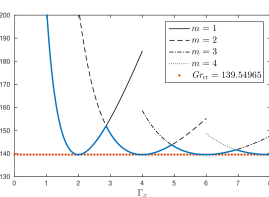
Figure 10: (Color Online) Critical Grashoff numbers for energy stability of the Couette solution for the two dimensional flow. The neutral curves for individual Fourier modes and the results from Hagstrom and Doering (2014) are also shown for comparison.

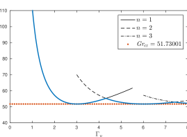
Figure 11: (Color Online) Critical Grashoff numbers for energy stability of the Couette solution for the three dimensional flow, under the assumption that the critical mode is independent of the streamwise direction. The neutral curves for individual Fourier modes and the results from Hagstrom and Doering (2014) are also shown for comparison.

Figures 10 and 11 show $\textit{Gr}_{\text{cr}}$ for the two and three dimensional flows as a function of the domain aspect ratios $\Gamma_{x}$ and $\Gamma_{y}$. As in Section V, we have assumed that the critical modes for the three dimensional flow are independent of the streamwise direction; this assumption is not necessary, but significantly simplifies the formulation of the SDP and reduces its computational cost. The figures also illustrate the neutral curves for each individual Fourier mode, which can be easily computed by considering only a single Fourier mode in the SDP. Note that, as one would expect, all pairs $(m,\Gamma_{x})$ achieving the same $\textit{Gr}_{\text{cr}}$ correspond to the same wavenumber $\alpha_{m}=2\pi m/\Gamma_{x}$ (respectively, $(n,\Gamma_{y})$ and $\beta_{n}=2\pi n/\Gamma_{y}$ for the three dimensional flow). In particular, the local minima correspond to $\alpha_{m}\approx 3.15$ and $\beta_{n}\approx 2.1$ for the two and three dimensional flows respectively, in excellent agreement with the results of Hagstrom and Doering (2014).

Strictly speaking, our results represent lower bounds on $\textit{Gr}_{\text{cr}}$ that account for the effect of all orthogonal modes of the velocity field, because the imposed LMIs are stronger conditions than the spectral constraint in (61). However, the optimal Gr computed with our SDP formulation converges (from below) to the exact $\textit{Gr}_{\text{cr}}$ as the number of Legendre coefficients in the expansions of $\bm{u}$ is increased. In fact, we obtained well converged results considering as few as 15 Legendre coefficients. This is confirmed by the figures: our results agree extremely well with those obtained with traditional methods Hagstrom and Doering (2014) (these reference results were computed treating the Fourier wavenumber as a continuous variable and hence correspond to the limit of infinite aspect ratio).

VII Conclusions

Using a novel numerical technique, we have computed near-optimal bounds on the dissipation coefficient for two and three dimensional shear flows driven by a surface stress. To our knowledge, this is the first time that near-optimal bounds are determined for flows with imposed boundary fluxes; previous attempts have only considered piecewise linear fields (e.g. Hagstrom and Doering (2014); Wittenberg and Gao (2010)). Our numerical results improve previous analytical bounds by more than 10 times at large Gr, and agree with the approximate computations carried out by Tang et al Tang et al. (2004). This confirms that flows driven by a surface stress are similar to those driven by a localized body force not only in terms of their energy stability boundaries Hagstrom and Doering (2014), but also as far as bounds on the dissipation coefficient are concerned.

While our bounds have been obtained considering a restricted class of background fields, we expect that no significant further improvements can be achieved by other numerical techniques and, in practice, our results can be considered optimal. Yet, it should be recognized that our bounds are only optimal within the variational formulation proposed by Hagstrom & Doering Hagstrom and Doering (2014). In fact, as suggested by Tang et al. Tang et al. (2004), it is unlikely that our bounds are achieved by any real flow. It is therefore of future interest to compare our bounds to scaling laws estimated via numerical simulations or experiments of the flow at high Gr (not available at the time of writing).

Finally, we emphasize the central role played by our numerical approach, which allowed us to avoid the technical complications that affect the classical variational framework when fixed-flux BCs must be imposed. Although the computational challenges related to the solution of SDPs at large Gr prevented us from reaching the asymptotic regime and estimating accurate scaling laws, the formulation of SDPs is generally attractive for the following two reasons. First, SDP relaxations can be derived systematically for a wide range of problems Fantuzzi and Wynn (2015b), not only of the type studied in this work. For instance, we have demonstrated that SDPs provide an efficient alternative to traditional methods, based on the solution of boundary-eigenvalue problems, in the context of energy stability. Second, the SDP is formulated in a rigorous manner, meaning that its feasible region corresponds to a set that is contained within the feasible set of the original infinite dimensional bounding problem. While the bounds presented in this work cannot be considered analytic results due to the numerical roundoff errors in the solution of the SDPs, the rigorous formulation of a finite dimensional problem represents a first step towards the construction of a fully computer-assisted proof of near-optimal bounds. For these reasons, we expect that if the technical difficulties related to solving SDPs in the asymptotic regime can be overcome by future work, semidefinite programming will provide a robust framework to solve bounding problems across a wide range of contexts.

Appendix A Properties of Legendre series

Let $W(\zeta)$ be defined for $\zeta\in[-1,1]$. We assume that $W$ has enough regularity such that $\frac{dW}{d\zeta}$ has a uniformly convergent Legendre expansion; for example, assume that $W$ is twice continuously differentiable Jackson (1930). Under the assumption of uniform convergence, the Legendre series

$$\begin{gathered}W=\sum_{n=0}^{\infty}\hat{w}_{n}\mathcal{L}_{n}(\zeta),\\ \frac{dW}{d\zeta}=\sum_{n=0}^{\infty}\hat{w}_{n}^{\prime}\mathcal{L}_{n}(\zeta),\end{gathered}$$ (62)

can be related using the fundamental theorem of calculus and the fact that

$$(2n+1)\mathcal{L}_{n}(\zeta)=\frac{d}{d\zeta}\left[\mathcal{L}_{n+1}(\zeta)-\mathcal{L}_{n-1}(\zeta)\right]$$ (63)

for all $n\geq 1$ Agarwal and O’Regan (2009). In fact, recalling that $\mathcal{L}_{0}(\zeta)\equiv 1$ and $\mathcal{L}_{1}(\zeta)\equiv\zeta$, we have

$$W(\zeta) =W(-1)+\int\limits_{-1}^{\zeta}\frac{dW}{dt}dt$$

$$=W(-1)+\sum_{n=0}^{\infty}{\hat{w}^{\prime}_{n}}\int\limits_{-1}^{\zeta}\mathcal{L}_{n}(t)dt$$

$$=W(-1)\cdot 1+{\hat{w}^{\prime}_{0}}(\zeta+1)$$

$$\quad+\sum_{n=1}^{\infty}\frac{\hat{w}^{\prime}_{n}}{2n+1}\int\limits_{-1}^{\zeta}\frac{d}{d\zeta}\left[\mathcal{L}_{n+1}(t)-\mathcal{L}_{n-1}(t)\right]dt$$

$$=W(-1)\mathcal{L}_{0}(\zeta)+{\hat{w}^{\prime}_{0}}\left[\mathcal{L}_{1}(\zeta)+\mathcal{L}_{0}(\zeta)\right]$$

$$\quad+\sum_{n=1}^{\infty}\frac{\hat{w}^{\prime}_{n}}{2n+1}\left[\mathcal{L}_{n+1}(\zeta)-\mathcal{L}_{n-1}(\zeta)\right],$$ (64)

where the boundary values cancel out since $\mathcal{L}_{n}(\pm 1)=(\pm 1)^{n}$. Rearranging the series and comparing coefficients we obtain the compatibility conditions

$$\hat{w}_{0} =W(-1)+\hat{w}^{\prime}_{0}-\frac{\hat{w}^{\prime}_{1}}{3},$$ (65)

$$\hat{w}_{n} =\frac{\hat{w}^{\prime}_{n-1}}{2n-1}-\frac{\hat{w}^{\prime}_{n+1}}{2n+3},\quad n\geq 1.$$

Moreover, it can be verified that

$$W(1)=W(-1)+\int\limits_{-1}^{1}\frac{dW}{d\zeta}d\zeta=W(-1)+2\hat{w}^{\prime}_{0}.$$ (66)

It is clear that these expressions can be applied recursively to relate $W(\zeta)$ and the boundary value $W(1)$ to higher order derivatives under suitable regularity assumptions.

Appendix B Legendre expansion of the spectral constraint

Substituting (38) into (26), recalling the definition of the remainder functions $\tilde{w}_{0}$, $\tilde{w}_{1}$, $\tilde{w}_{2}$, and using the orthogonality of the Legendre polynomials Zeidler (1995) we obtain

$$\mathcal{Q}\{W,\phi\} =\frac{16}{\alpha^{2}}\sum_{n=0}^{N+P+3}\frac{2|\hat{w}^{\prime\prime}_{n}|^{2}}{2n+1}+8\sum_{n=0}^{N+1}\frac{2|\hat{w}^{\prime}_{n}|^{2}}{2n+1}$$

$$\quad+\alpha^{2}\sum_{n=0}^{N}\frac{2|\hat{w}_{n}|^{2}}{2n+1}-\text{\rm Im}\left(\mathcal{P}\right)+\mathcal{R}.$$ (67)

Here, $\mathcal{R}=\mathcal{R}\{\tilde{w}_{0},\tilde{w}_{1},\tilde{w}_{2},\phi\}$ is as in (IV.3) and

$$\mathcal{P}:= \frac{8}{\alpha}\sum_{m=0}^{N+1}\sum_{n=0}^{\infty}\sum_{p=0}^{P}\hat{w}^{\prime}_{m}\hat{w}_{n}^{*}\hat{\phi}_{p}\Lambda_{mnp}$$

$$+\frac{8}{\alpha}\sum_{m=N+2}^{\infty}\sum_{n=0}^{N}\sum_{p=0}^{P}\hat{w}^{\prime}_{m}\hat{w}_{n}^{*}\hat{\phi}_{p}\Lambda_{mnp},$$ (68)

where

$$\Lambda_{mnp}=\int\limits_{-1}^{1}\mathcal{L}_{m}(\zeta)\mathcal{L}_{n}(\zeta)\mathcal{L}_{p}(\zeta)d\zeta.$$ (69)

Applying the compatibility conditions (39) to the first three terms of (67) we can find a real, symmetric, positive definite matrix $\bm{Q}_{1}$ such that

$$\left(\bm{\hat{w}}^{\prime\prime}\right)^{\dagger}\bm{Q}_{1}\bm{\hat{w}}^{\prime\prime}=\,\, \frac{16}{\alpha^{2}}\sum_{n=0}^{N+P+3}\frac{2|\hat{w}^{\prime\prime}_{n}|^{2}}{2n+1}$$

$$+8\sum_{n=0}^{N+1}\frac{2|\hat{w}^{\prime}_{n}|^{2}}{2n+1}+\alpha^{2}\sum_{n=0}^{N}\frac{2|\hat{w}_{n}|^{2}}{2n+1}.$$ (70)

Moreover, since $\Lambda_{mnp}=0$ if $m-n+p<0$ or $n-m+p<0$ Dougall (1953), the infinite sums over $n$ and $m$ in $\mathcal{P}$ can be truncated to $n\leq N+P+1$ and $m\leq N+P$ respectively. Calculating $\Lambda_{mnp}$ as in Dougall (1953) and letting

$$\bm{\Phi}_{mn}(\bm{\hat{\phi}}):=\frac{8}{\alpha}\sum_{p=0}^{P}\hat{\phi}_{p}\Lambda_{mnp}$$ (71)

we can write

$$\mathcal{P}= \sum_{m=0}^{N+1}\sum_{n=0}^{N+P+1}\hat{w}^{\prime}_{m}\hat{w}_{n}^{*}\bm{\Phi}_{mn}(\bm{\hat{\phi}})$$

$$+\sum_{m=N+2}^{N+P}\sum_{n=0}^{N}\hat{w}^{\prime}_{m}\hat{w}_{n}^{*}\bm{\Phi}_{mn}(\bm{\hat{\phi}}).$$ (72)

It should be understood that the second term is zero if $P<2$. Moreover, note that the $\bm{\Phi}_{mn}$’s are linear in $\bm{\hat{\phi}}$. Using (39) we can then write $\mathcal{P}=\left(\bm{\hat{w}}^{\prime\prime}\right)^{\dagger}\bm{Q}_{2}(\bm{\hat{\phi}})\bm{\hat{w}}^{\prime\prime}$ for a suitably defined real matrix $\bm{Q}_{2}(\bm{\hat{\phi}})$ whose entries are linear combinations of the $\bm{\Phi}_{mn}$’s (and are therefore linear in $\bm{\hat{\phi}}$). We remark that, contrary to $\bm{Q}_{1}$, the matrix $\bm{Q}_{2}(\bm{\hat{\phi}})$ is not symmetric.

Appendix C A lower bound on $\mathcal{R}$

In order to derive the lower bound on $\mathcal{R}$ stated in (IV.3), we start by deriving a relation between $\left\|\tilde{w}_{0}\right\|_{2}$, $\left\|\tilde{w}_{1}\right\|_{2}$ and $\left\|\tilde{w}_{2}\right\|_{2}$. Using (39) and the elementary inequality $(a-b)^{2}\leq 2a^{2}+2b^{2}$ we can write

$$\left\|\tilde{w}_{1}\right\|_{2}^{2} =\sum_{n=N+2}^{\infty}\frac{2\left|\hat{w}_{n}^{\prime}\right|^{2}}{2n+1}$$ (73)

$$\leq\sum_{n=N+2}^{\infty}\frac{4\left|\hat{w}_{n-1}^{\prime\prime}\right|^{2}}{(2n-1)^{2}(2n+1)}$$

$$\quad+\sum_{n=N+2}^{\infty}\frac{4\left|\hat{w}_{n+1}^{\prime\prime}\right|^{2}}{(2n+1)(2n+3)^{2}}.$$

Defining a matrix $\bm{H}_{1}$ such that

$$(\bm{\hat{w}}^{\prime\prime})^{\dagger}\bm{H}_{1}\bm{\hat{w}}^{\prime\prime} =\sum_{n=N+2}^{N+P+4}\frac{4\left|\hat{w}_{n-1}^{\prime\prime}\right|^{2}}{(2n-1)^{2}(2n+1)}$$

$$\quad+\sum_{n=N+2}^{N+P+2}\frac{4\left|\hat{w}_{n+1}^{\prime\prime}\right|^{2}}{(2n+1)(2n+3)^{2}}$$ (74)

and letting

$$\lambda_{1}=\frac{4}{[2(N+P+4)-1][2(N+P+4)+3]}$$ (75)

it can be verified that

$$\left\|\tilde{w}_{1}\right\|_{2}^{2}\leq(\bm{\hat{w}}^{\prime\prime})^{\dagger}\bm{H}_{1}\bm{\hat{w}}^{\prime\prime}+\lambda_{1}\left\|\tilde{w}_{2}\right\|_{2}^{2}.$$ (76)

Note that $\left\|\bm{H}_{1}\right\|_{F}\sim\mathcal{O}(N^{-3})$ and $\lambda_{1}\sim\mathcal{O}(N^{-2})$. Using similar ideas, we can express $\left\|\tilde{w}_{0}\right\|_{2}^{2}$ in terms of the coefficients $\hat{w}_{n}^{\prime}$, $n\leq N+1$ and $\left\|\tilde{w}_{1}\right\|_{2}^{2}$. We then use (39) and (76) to construct a matrix $\bm{H}_{0}$ and a constant $\lambda_{0}$ such that

$$\left\|\tilde{w}_{0}\right\|_{2}^{2}\leq(\bm{\hat{w}}^{\prime\prime})^{\dagger}\bm{H}_{0}\bm{\hat{w}}^{\prime\prime}+\lambda_{0}\left\|\tilde{w}_{2}\right\|_{2}^{2}.$$ (77)

Given the scaling estimates of $\bm{H}_{1}$ and $\lambda_{1}$ and the compatibility conditions (39), it is relatively straightforward to see that $\left\|\bm{H}_{0}\right\|_{F}\sim\mathcal{O}(N^{-5})$ and $\lambda_{0}\sim\mathcal{O}(N^{-4})$.

Let us now turn our attention to the functional $\mathcal{R}$ defined as in (IV.3). Clearly, we have the lower bound

$$\mathcal{R}\geq\frac{16}{\alpha^{2}}\left\|\tilde{w}_{2}\right\|_{2}^{2}-\frac{8}{\alpha}\left\|\frac{d\phi}{d\zeta}\right\|_{\infty}\int\limits_{-1}^{1}\left|\text{\rm Im}\left(\tilde{w}_{1}\tilde{w}_{0}^{*}\right)\right|d\zeta.$$ (78)

Using Young’s inequality, followed by (76) and (77), we find that for any $\delta>0$

$$\int\limits_{-1}^{1}\left|\text{\rm Im}\left(\tilde{w}_{1}\tilde{w}_{0}^{*}\right)\right|d\zeta\leq (\bm{\hat{w}}^{\prime\prime})^{\dagger}\left[\frac{\delta}{2}\bm{H}_{0}+\frac{1}{2\delta}\bm{H}_{1}\right]\bm{\hat{w}}^{\prime\prime}$$

$$+\left[\frac{\delta}{2}\lambda_{0}+\frac{1}{2\delta}\lambda_{1}\right]\left\|\tilde{w}_{2}\right\|_{2}^{2}.$$ (79)

Letting

$$\delta=\sqrt{\frac{\lambda_{1}}{\lambda_{0}}},$$ (80)

$$\bm{R}:=\frac{8}{\alpha}\left[\frac{\delta}{2}\bm{H}_{0}+\frac{1}{2\delta}\bm{H}_{1}\right],$$ (81)

$$\kappa=\frac{\alpha}{2}\sqrt{\lambda_{0}\lambda_{1}},$$ (82)

and using (32) finally proves (IV.3).

Appendix D Necessity of conditions (52)

Let us consider the problem of enforcing the constraint $\Psi\geq 0$, where $\Psi$ is as in equation (IV.3), subject to (48). Condition (48a) can be enforced using (49) as explained in Section IV.3, and the problem reduces to showing that

$$\begin{bmatrix}\text{\rm Re}\left(\bm{\hat{\omega}}\right)\\ \text{\rm Im}\left(\bm{\hat{\omega}}\right)\end{bmatrix}^{T}\bm{Q}(\bm{\hat{\phi}})\begin{bmatrix}\text{\rm Re}\left(\bm{\hat{\omega}}\right)\\ \text{\rm Im}\left(\bm{\hat{\omega}}\right)\end{bmatrix}+\frac{16}{\alpha^{2}}\left(1-\kappa\,\|\bm{\hat{\phi}}\|_{1}\right)\left\|\tilde{w}_{2}\right\|^{2}_{2}\geq 0$$ (83)

for all $\bm{\hat{\omega}}\in\mathbb{R}^{N+P+3}$ and $\tilde{w}_{2}(1)$ satisfying (48b). This condition can be rewritten with the help of (49) as

$$\tilde{w}_{2}(1)=-\bm{1}^{T}\bm{A}\bm{\hat{\omega}},$$ (84)

where $\bm{1}$ is a column vector of ones of length $N+P+4$.

The conditions in (52) are clearly sufficient for (83), since they enforce the non-negativity of each of the two terms separately regardless of whether $\bm{\hat{\omega}}$ and $\tilde{w}_{2}$ satisfy (84). Moreover, it is not difficult to see that (52b) is also necessary. This follows because $\bm{\hat{\omega}}=0$ is an admissible choice and there exists $\tilde{w}_{2}\neq 0$ that satisfies $\tilde{w}_{2}(1)=0$.

To show that (52a) is also necessary, for any fixed $\bm{\hat{\omega}}$ we construct a sequence of remainder functions $\tilde{w}_{2}$ satisfying (84) showing that when (83) holds, the term

$$\begin{bmatrix}\text{\rm Re}\left(\bm{\hat{\omega}}\right)\\ \text{\rm Im}\left(\bm{\hat{\omega}}\right)\end{bmatrix}^{T}\bm{Q}(\bm{\hat{\phi}})\begin{bmatrix}\text{\rm Re}\left(\bm{\hat{\omega}}\right)\\ \text{\rm Im}\left(\bm{\hat{\omega}}\right)\end{bmatrix}$$

must be non-negative. In fact, given $\bm{\hat{\omega}}$, consider the admissible remainder functions

$$\tilde{w}_{2}^{(m)}(\zeta):=\left(-\bm{1}^{T}\bm{A}\bm{\hat{\omega}}\right)\mathcal{L}_{m}(\zeta)$$ (85)

for $m\geq N+P+4$. For such a function, we have

$$\left\|\tilde{w}_{2}\right\|^{2}_{2} =\frac{2|\bm{1}^{T}\bm{A}\bm{\hat{\omega}}|^{2}}{2m+1}$$

$$=\frac{2}{2m+1}\bm{\hat{\omega}}^{\dagger}\left(\bm{A}^{T}\bm{1}\bm{1}^{T}\bm{A}\right)\bm{\hat{\omega}}$$

$$\leq\lambda_{\mathrm{max}}\left(\bm{A}^{T}\bm{1}\bm{1}^{T}\bm{A}\right)\left\|\bm{\hat{\omega}}\right\|^{2},$$ (86)

where $\lambda_{\mathrm{max}}(\cdot)$ denotes the maximum eigenvalue of a matrix. Note that $\lambda_{\mathrm{max}}\left(\bm{A}^{T}\bm{1}\bm{1}^{T}\bm{A}\right)$ is a fixed positive quantity for any fixed $N$ and $P$. If (83) holds, then

$$\begin{bmatrix}\text{\rm Re}\left(\bm{\hat{\omega}}\right)\\ \text{\rm Im}\left(\bm{\hat{\omega}}\right)\end{bmatrix}^{T}\bm{Q}(\bm{\hat{\phi}})\begin{bmatrix}\text{\rm Re}\left(\bm{\hat{\omega}}\right)\\ \text{\rm Im}\left(\bm{\hat{\omega}}\right)\end{bmatrix} \geq-\frac{16}{\alpha^{2}}\left(1-\kappa\,\|\bm{\hat{\phi}}\|_{1}\right)\left\|\tilde{w}_{2}\right\|^{2}_{2}$$

$$\geq-\frac{C(\bm{\hat{\phi}})}{2m+1}\left\|\bm{\hat{\omega}}\right\|^{2},$$ (87)

where the non-negative term

$$C(\bm{\hat{\phi}}):=\frac{32}{\alpha^{2}}\lambda_{\mathrm{max}}\left(\bm{A}^{T}\bm{1}\bm{1}^{T}\bm{A}\right)\left(1-\kappa\,\|\bm{\hat{\phi}}\|_{1}\right)$$ (88)

only depends on the choice of $\bm{\hat{\phi}}$, and can therefore be considered fixed. Since (D) holds for any $\bm{\hat{\omega}}$, we must have

$$\lambda_{\mathrm{min}}\left[\bm{Q}(\bm{\hat{\phi}})\right]\geq-\frac{C(\bm{\hat{\phi}})}{2m+1},$$ (89)

where $\lambda_{\mathrm{min}}(\cdot)$ denotes the minimum eigenvalue of a matrix. Letting $m\to\infty$ shows that $\bm{Q}(\bm{\hat{\phi}})$ must be positive semidefinite, meaning that (52a) is a necessary condition for (83) to hold for all $\bm{\hat{\omega}}$’s and $\tilde{w}_{2}$’s subject to (84).

References

• Constantin and Doering (1995) P. Constantin and C. R. Doering,  Phys. D Nonlinear Phenom. 82, 221 (1995).
• Doering and Constantin (1992) C. R. Doering and P. Constantin,  Phys. Rev. Lett. 69, 1648 (1992).
• Doering and Constantin (1994) C. R. Doering and P. Constantin,  Phys. Rev. E 49, 4087 (1994).
• Nicodemus et al. (1998a) R. Nicodemus, S. Grossmann,  and M. Holthaus,  J. Fluid Mech. 363, 281 (1998a).
• Nicodemus et al. (1998b) R. Nicodemus, S. Grossmann,  and M. Holthaus,  J. Fluid Mech. 363, 301 (1998b).
• Nicodemus et al. (1997) R. Nicodemus, S. Grossmann,  and M. Holthaus,  Phys. Rev. E 56, 6774 (1997).
• Doering and Constantin (1996) C. R. Doering and P. Constantin,  Phys. Rev. E 53, 5957 (1996).
• Whitehead and Doering (2011) J. P. Whitehead and C. R. Doering, Phys. Rev. Lett. 106, 244501 (2011).
• Wen et al. (2013) B. Wen, G. P. Chini, N. Dianati,  and C. R. Doering,  Phys. Lett. A 377, 2931 (2013).
• Wen et al. (2015) B. Wen, G. P. Chini, R. R. Kerswell,  and C. R. Doering,  Phys. Rev. E 92, 043012(13) (2015).
• Hagstrom and Doering (2010) G. Hagstrom and C. R. Doering,  Phys. Rev. E 81, 047301 (2010).
• Hagstrom and Doering (2014) G. I. Hagstrom and C. R. Doering,  J. Nonlinear Sci. 24, 185 (2014).
• Wittenberg and Gao (2010) R. W. Wittenberg and J. Gao, Eur. Phys. J. B 76, 565 (2010).
• Courant and Hilbert (1953) R. Courant and D. Hilbert, Methods of Mathematical Physics, 1st ed., Vol. 1 (Interscience Publisher Inc., New York, 1953).
• Giaquinta and Hildebrandt (2004) M. Giaquinta and S. Hildebrandt,  Calculus of Variations I, 2nd ed. (Springer-Verlag, Berlin, 2004).
• Fantuzzi and Wynn (2015a) G. Fantuzzi and A. Wynn,  Phys. Lett. A 379, 23 (2015a).
• Tang et al. (2004) W. Tang, C. P. Caulfield,  and W. R. Young,  J. Fluid Mech. 510, 333 (2004).
• Boyd et al. (1994) S. Boyd, L. El Ghaoui, E. Feron,  and V. Balakrishnan,  Linear Matrix Inequalities In System And Control Theory (SIAM, Philadelphia, 1994).
• Boyd and Vandenberghe (2004) S. Boyd and L. Vandenberghe,  Convex Optimization (Cambridge University Press, Cambridge, 2004).
• Vandenberghe and Boyd (1996) L. Vandenberghe and S. Boyd,  SIAM Rev. 38, 49 (1996).
• Zeidler (1995) E. Zeidler,  Applied Functional Analysis - Applications to Mathematical Physics, 1st ed. (Springer-Verlag, New York, 1995).
• Jackson (1930) D. Jackson, The Theory of Approximation (American Mathematical Society, New York, 1930).
• Agarwal and O’Regan (2009) R. P. Agarwal and D. O’Regan,  Ordinary and Partial Differential Equations, With Special Functions, Fourier Series and Boundary Value Problems (Springer-Verlag, New York, 2009).
• Fantuzzi and Wynn (2015b) G. Fantuzzi and A. Wynn,  “Semidefinite Relaxation of Quadratic Functional Inequalities,”  (2015b), in preparation .
• Löfberg (2004) J. Löfberg, in IEEE Int. Symp. Comput. Aided Control Syst. Des. (Taipei, 2004) pp. 284 – 289.
• Sturm (1999) J. F. Sturm,  Optim. Methods Softw. 11, 625 (1999).
• Fukuda et al. (2000) M. Fukuda, M. Kojima, M. Kazuo,  and K. Nakata,  SIAM J. Optim. 11, 647 (2000).
• Nakata et al. (2003) K. Nakata, K. Fujisawa, M. Fukuda, M. Kojima,  and K. Murota,  Math. Program. 95, 303 (2003).
• Burer and Monteiro (2003) S. Burer and R. D. C. Monteiro,  Math. Program. Ser. B 95, 329 (2003).
• Burer and Monteiro (2005) S. Burer and R. D. C. Monteiro,  Math. Program. 103, 427 (2005).
• Burer and Choi (2006) S. Burer and C. Choi,  Optim. Methods Softw. 21, 493 (2006).
• Wen et al. (2010) Z. Wen, D. Goldfarb,  and W. Yin,  Math. Program. Comput. 2, 203 (2010).
• Sun et al. (2014) Y. Sun, M. S. Andersen,  and L. Vandenberghe,  SIAM J. Optim. 24, 873 (2014).
• Dougall (1953) J. Dougall,  Proc. Glas. Math. Assoc. 1, 121 (1953).