A simple phenomenological model for describing the normal state single particle spectral function of high temperature superconductors

Abstract

Describing the normal state single particle spectral function line shapes of high temperature superconductors remains an important goal in condensed matter physics. RecentlyMatsuyama and Gweon (2013), we have proposed a phenomenological extremely correlated Fermi liquid (pECFL) model that promises to accomplish this goal and that is uniquely distinguished from other models. Here, we present an even more simplified phenomenological model, which we refer to as the aECFL model, that performs practically at the same level as the pECFL model. Noting the similarities of the aECFL model and the pECFL model, as well as the differences between the two models, we emphasize the universal significance of the $\omega$-dependence of the so-called caparison factor in the ECFL model.

I Introduction

In the study of high temperature superconductors, the interpretation of the angle resolved photoelectron spectroscopy (ARPES) data is a major thread of research, which remains vitally important. Perhaps one of the most challenging, but yet the most basic, subject in this line of research is that of establishing the correct model in the normal state Anderson (2006).

In our previous work Matsuyama and Gweon (2013), we have introduced a phenomenological model, the phenomenological extremely correlated electron Fermi-liquid (pECFL) model, that is successful in explaining both the energy distribution curves (EDCs) and the momentum distribution curves (MDCs) of ARPES data on equal footing. The characteristics of this work can be summarized as follows: (1) High quality fits of ARPES data are easily obtained for both EDCs and MDCs within a simple model. (2) The model is based on a Fermi liquid theory, albeit an unusual one Shastry (2011a, b), in contrast to other well-known theoretical models that strive to fit ARPES data, such as the hidden Fermi liquid (HFL) theory Anderson (2006) and the marginal Fermi liquid (MFL) theory Varma et al. (1989), both of which are non-Fermi liquid theories. (3) The model is able to explain the universal EDC line shape (characterized by the strong asymmetry) and the material-dependent non-universal MDC line shape (which can be asymmetric or symmetric) thanks to one central feature, the “caparison factor.” In contrast, other theories tend to produce always symmetric MDCs (MFL), or always strongly asymmetric MDCs and insufficiently asymmetric EDCs (HFL).

Our pECFL model Matsuyama and Gweon (2013) was the outcome of the evolution of a model Gweon et al. (2011) that was inspired directly from the original many body theory Shastry (2011a). The achievement of the pECFL model is impressive, and the construction of the pECFL model was soundly based on the basic principles such as the positivity of the spectral function and the causality of the Green’s function. Nevertheless, one might wonder whether it is possible to come up with an alternative model, as the momentum dependent pECFL (MD-pECFL) model described in our previous work Matsuyama and Gweon (2013) can be viewed as somewhat complicated.

In this work, we show that indeed an alternative model is possible. We name this new phenomenological model the aECFL model, where “a” stands for the parameter $a$, the key parameter that governs the behavior of the model. Also, one may interpret “a” to mean “alternative.”

As we shall see below, while the pECFL model remains more sound in its construction, the aECFL model has the advantage of being simpler while being able to reproduce all results of the pECFL model. As a matter of principle, the aECFL model has the dangerous possibility of breaking the positivity of the spectral function, if the value of $a$ becomes too large. Fortunately, we find that the values of $a$ for both Bi₂Sr₂CaCu₂O_8+δ (Bi2212) and La_2-xSr_xCuO₄ (LSCO) remain small. In this sense, we may regard the aECFL model and the pECFL model as being practically equivalent.

II The line shape fits of Bi2212 data

We shall present the aECFL model fit results for Bi2212 before presenting the model. All ECFL model parameters are the same as those used in our previous work Gweon et al. (2011); Matsuyama and Gweon (2013). For the aECFL model, we have a new parameter $a$, which effectively replaces the two parameters $a_{1}$ and $a_{2}$ in the pECFL model Matsuyama and Gweon (2013). So, below, we focus on the parameter $a$.

II.1 EDC description

Fig. 1 shows the EDC curves of Bi2212 taken along the nodal direction fit with the aECFL model. These data are identical with those of our previous work Matsuyama and Gweon (2013).

We see that the value of $a$ does not affect the quality of EDC fits at all. All fits shown in Fig. 1 are equivalent in quality, where the parameter $a$ was taken to be as large as 0.5.

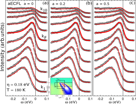
Figure 1: Line shape fits of EDCs for Bi2212 ($x$ = 0.15, T = 180 K) (a) aECFL ($a$ = 0) (b) aECFL ($a$ = 0.2) (c) aECFL ($a$ = 0.5) all other fitting parameter values are identical with those used in our previous work Matsuyama and Gweon (2013). The inset in (b) shows the data range used for EDC fits (E) and MDC fits (M; next figure).

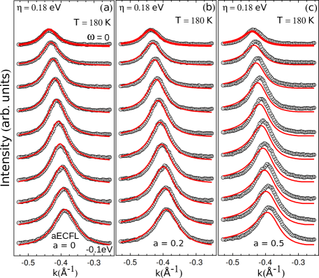
Figure 2: Line shape fits of MDCs for Bi2212 ($x=$ 0.15, T = 180 K) (a) aECFL ($a$ = 0) (b) aECFL ($a$ = 0.2) (c) aECFL ($a$ = 0.5) all other fitting parameter values are identical with those used in our previous work Matsuyama and Gweon (2013).

II.2 MDC description

The situation becomes quite different when we examine MDCs for Bi2212. For MDCs, $a$ makes a crucial difference. As Fig. 2 shows, $a=0$ gives the best fit. The fit degrades slightly, but noticeably, when $a=0.2$. The degradation is severe and unmistakable when $a=0.5$. If $a$ goes past 0.5, the degradation becomes even more severe.

These findings are in good agreement with our previous work Matsuyama and Gweon (2013), as we shall see shortly. At this point, it suffices to note that the symmetry of the MDCs observed for Bi2212 can be described only with $a=0$.

III The $a$ECFL model

To motivate our new model, let us go back to the original ECFL model, the simple ECFL (sECFL) model Gweon et al. (2011):

$$G(\vec{k},\omega) =\frac{Q_{n}}{\gamma_{n}}+\frac{\mathcal{C}_{n}(\vec{k},\omega)}{\omega-\varepsilon(\vec{k})-\Phi(\omega)},$$ (1)

$$\mathcal{C}_{n}(\vec{k},\omega) =Q_{n}\left(1-\frac{\omega-\varepsilon(\vec{k})}{\gamma_{n}}\right).$$ (sECFL) (2)

where $G$ is the single-particle Green’s function and $C_{n}$ is the so-called “caparison factor.” $Q_{n}=1-(n/2)$ where $n$ is the number of electrons per unit cell. $\gamma_{n}=4Q_{n}\Delta_{0}/n^{2}$ and $\Delta_{0}$ ($\sim 0.1$ eV) is an energy scale parameter for $C_{n}$. $\varepsilon(\vec{k})$ is the one-electron band dispersion relation. $\Phi$ is the Dyson self energy of the underlying Fermi liquid, which was termed the auxiliary Fermi liquid, whose full Green’s function is given by $1/(\omega-\varepsilon(\vec{k})-\Phi(\omega))$.

In our previous work Matsuyama and Gweon (2013), our goal was to develop a systematic way to deal with the problem that the above caparison factor, if used for $\omega\gg\varepsilon(\vec{k})$ (as for an MDC analysis), becomes a negative value, leading to an unphysical negative value for the spectral function $A(\vec{k},\omega)=\frac{1}{\pi}\mathrm{Im}\,G$.

The aECFL idea arises from a simpler idea for remedy to this problem. In using the above theory to fit ARPES data, the problem lies with the $\varepsilon(\vec{k})$ factor, since $\omega$ is limited to mostly negative values for ARPES data. So, what if we just scale $\varepsilon(\vec{k})\rightarrow a\varepsilon(\vec{k})$ with $0\leq a\leq 1$?

This way, we obtain the caparison factor for the aECFL

$$\mathcal{C}_{n}(\vec{k},\omega) =Q_{n}\left(1-\frac{\omega-a\varepsilon(\vec{k})}{\gamma_{n}}\right).$$ (aECFL) (3)

In comparison to our previous work Matsuyama and Gweon (2013), this caparison factor is much simpler, but we cannot assure the same rigorous analytical properties (the sum rule and the non-negativity) of the spectral function as we were able to do with our pECFL model Matsuyama and Gweon (2013). Here, our goal is rather to stay with the original spirit of the sECFL model, i.e., the construction of a low energy model that can describe well the data near the Fermi surface. The strength of the aECFL model is that it can describe MDCs well (as we show here), which the original sECFL could not do. Also, it is tempting to make a guess that $a$ could arise through some renormalization process although it remains to be seen whether a microscopic calculation will in fact produce such a scaling factor.

Note that, when $a=0$, we recover the momentum-independent (MI) pECFL model, used in our previous work Matsuyama and Gweon (2013). If $a=1$, then we recover the sECFL model.

Therefore, it is not surprising at all that the $a=0$ aECFL model does an excellent job describing EDCs and MDCs for Bi2212, since we have already shown that the MI-pECFL model provides a good description for the Bi2212 data Matsuyama and Gweon (2013).

As we will show in the next section, it is possible to quantify this finding further using the aECFL model. Also, we are able to fit the LSCO data with the same aECFL model Here are the main results: $a=0\pm 0.03$ for Bi2212 and $a=0.2\pm 0.08$ for LSCO.

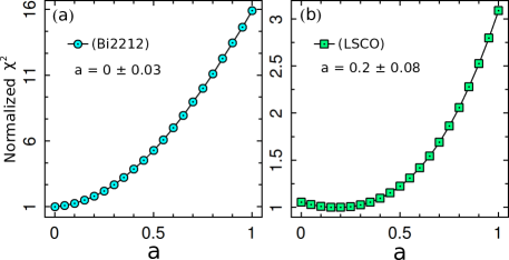
Figure 3: $\chi^{2}$ variation as a function of $a$. For each value of $a$, the $\chi^{2}$ value averaged over all EDCs and MDCs are plotted. (a) Bi2212 ($x=$ 0.15, T = 180 K). (b) LSCO ($x=$ 0.15, T = 20 K).

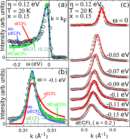
Figure 4: aECFL line shape fits ($a=0.2$) to the data taken along the nodal direction of optimally doped LSCO Yoshida et al. (2007) ($x=0.15$, T= 20 K) and their comparison with other ECFL models. (a) EDC fits at k = $k_{F}$, (b) MDC fits at $\omega=-0.1$ eV, (c) MDC line shape fits for $\omega$ values ranging from 0 to $-0.15$ eV. For the exact range of the fit data, see the next figure (Fig. 5(d)).

IV determination of $a$ value

Fig. 3 shows the values of $\chi^{2}$ plotted as a function of the parameter $a$ for Bi2212 (a) and LSCO (b). The displayed $\chi^{2}$ value is the average of the average $\chi^{2}$ value of EDC fits and the average $\chi^{2}$ value of MDC fits. We determined the value of $\chi^{2}$ in the data range used for EDC fits, and we will describe this reason in the next section when we present the line shape fits of LSCO data. As evidenced by these graphs, the qualities of fits degrade significantly as the parameter $a$ becomes large.

To determine the best value of the parameter $a$ for each material shown in Fig. 3, we read the $a$ value for the minimum position of $\chi^{2}$. We find $a=0$ for Bi2212 and $a=0.2$ for LSCO. As Fig. 3 shows, the minimum position of $\chi^{2}$ is well-defined, giving only a small uncertainty, $\pm 0.03$, for the estimated $a$ value. We can estimate the uncertainty of $a$ further by adjusting the fit ranges of EDCs and MDCs and then examining the new values of $a$. The adjustment of the fitting ranges by $\pm 20\%$ resulted in little change to the $\chi^{2}$ plot of Bi2212, while the minimum position of $\chi^{2}$ of LSCO shifted by $\pm 0.08$. Therefore, the uncertainty for $a$ value is $\pm 0.03$ for Bi2212 and $\pm 0.08$ for LSCO.

As noted already, regardless of $a$ values, all ECFL model parameter values were held fixed as those same values used in our previous work Matsuyama and Gweon (2013). It is also worth noting that the bare Fermi velocity is treated as a model-dependent, i.e., $a$-dependent, quantity as in the same work Matsuyama and Gweon (2013). Its value (times $\hbar$, which is set to 1 in our work) for Bi2212 was varied linearly from 6.3 eVÅ ($a=0$; MI-pECFL) to 5.5 eVÅ ($a=1$; sECFL) and that for LSCO were varied linearly from 5.5 eVÅ ($a=0$; MI-pECFL) to 4 eVÅ ($a=1$; pECFL).

V The line shape fits of LSCO data

Next, we present the fits of LSCO data by the aECFL model in Fig. 4. Fig. 4(a) shows the EDC fitting by the aECFL model at the Fermi momentum. Fitting quality comparison between all phenomenological ECFL models show no difference, and fits are all equally successful. Fig. 4(b) shows the MDC fitting at $\omega=-0.1$ eV. Here, we see that the fit quality varies over different ECFL models. The aECFL fit is very good, almost as good as the best fit (the MD-pECFL fit). A more quantitative discussion of the fit quality will be presented below.

In Fig. 4(c), we show MDC fits by the aECFL model at various energy values. The aECFL model successfully describes the asymmetry in MDC curves which becomes more obvious for higher energy values ($-\omega\gtrsim 80$ meV). As the theory is for the normal state, and the data are for the superconducting state, the comparison between theory and experiment is not straightforward. As we argued in our previous work Matsuyama and Gweon (2013), however, the comparison is still quite meaningful at high energy values, where the measured electronic structure remains essentially unchanged in the normal state. Even at low energy, the comparison between theory and experiment remains quite good.

The description of the LSCO data with the aECFL model is as good as the description with the pECFL model in our previous work Matsuyama and Gweon (2013). To examine the quality of the aECFL fit a bit more in depth, we now examine the $\chi^{2}$ values for different ECFL models.

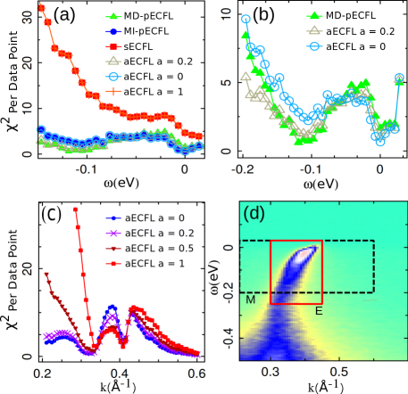
Figure 5: (a) Comparison of $\chi^{2}$ values for MDC fits using various ECFL models. (b) The same plot as (a) but for only three ECFL models, showing details. (c) $\chi^{2}$ values for EDC fits by aECFL. (d) LSCO data along the nodal direction Yoshida et al. (2007) ($x=0.15$, T = 20 K). Two rectangles show the data ranges used for the MDC fits (M) and the EDC fits (E), to produce analysis results reported in this paper. However, one exception is panel (c) of this figure, where EDC fits are shown for a much wider ranges of $k$.

In Fig. 5, we show $\chi^{2}$ value per data point (a,b,c), as well as the data ranges used in our fits (d). In Fig. 5(a), we see that the aECFL models with the value of $a$ from 0 to 1 are able to reproduce the same good MDC fits as pECFL fits. On a closer look, we can discern differences, as we can do with Fig. 5(b). In this figure, we can see that on average the aECFL model with $a=0.2$ performs the best, when we focus on the important high energy range ($-\omega\gtrsim 80$ meV). When $a$ increases, the fit quality degrades: this is shown dramatically for the $a=1$ case (for which aECFL becomes sECFL) in panel (a).

When we look at the $\chi^{2}$ values for EDC fits, the same pathology for large $a$ can be noticed. In panel (c), we show $\chi^{2}$ values for EDC fits. For $k$ values corresponding to deep inside the Fermi surface ($k\lesssim 0.3$ Å^-1), we see that the fit quality degrades dramatically when $a$ increases beyond about 0.5. The origin of this pathology is, of course, the sign problem of the caparison factor of the sECFL model, as we discussed above.

Within the aECFL formalism presented here, therefore, we limited the momentum range used for EDC fits to that indicated in Fig. 5(d) to avoid the deep-inside-Fermi-surface region. We also emphasize that a large value of $a$ ($\gtrsim 0.5$) would make the aECFL model ill-defined, and so care must be taken that the application of this model be limited to small $a$ values.

VI Conclusion

In this work, we showed that it is possible to construct an alternative model, called aECFL, to our previous phenomenological ECFL models. The aECFL model is simple and is as successful as our previously reported models.

The dichotomy of EDC line shape and MDC line shape has been explained well by our previous and current models, and other theory has been proposed Ovchinnikov et al. (2014) to explain the same. The particularly nice aspect of the current aECFL model is that (1) the asymmetry of EDC is guaranteed by the strong $\omega$ dependence of the caparison factor, while (2) the degree of the asymmetry of MDC is tuned by the $a$ parameter.

References

- Matsuyama and Gweon (2013) K. Matsuyama and G.-H. Gweon, Physical Review Letters 111, 246401 (2013).
- Anderson (2006) P. W. Anderson, Nat Phys 2, 626 (2006).
- Shastry (2011a) B. S. Shastry, Physical Review Letters 107, 056403 (2011a).
- Shastry (2011b) B. S. Shastry, Physical Review B 84, 165112 (2011b).
- Varma et al. (1989) C. M. Varma, P. B. Littlewood, S. Schmitt-Rink, E. Abrahams, and A. E. Ruckenstein, Physical Review Letters 63, 1996 (1989).
- Gweon et al. (2011) G.-H. Gweon, B. S. Shastry, and G. D. Gu, Physical Review Letters 107, 056404 (2011).
- Note (1) Throughout this paper, we use , and so, e.g., and have the same dimension.
- Note (2) As in our previous work, we work with the advanced Green’s function.
- Note (3) Private communication, R. R. P. Singh.
- Note (4) In contrast, note that in our previous work, the MD-pECFL model, used to fit the LSCO data, and the MI-pECFL model, used to fit the Bi2212 data, were rather different. The MD-pECFL model interpolates between the sECFL model and a scaled auxiliary FL model, and it does not converge to the MI-pECFL model for any parameter values.
- Yoshida et al. (2007) T. Yoshida, X. J. Zhou, D. H. Lu, S. Komiya, Y. Ando, H. Eisaki, T. Kakeshita, S. Uchida, Z. Hussain, Z.-X. Shen, and A. Fujimori, Journal of Physics: Condensed Matter 19, 125209 (2007).
- Ovchinnikov et al. (2014) S. G. Ovchinnikov, E. I. Shneyder, and A. A. Kordyuk, Phys. Rev. B 90, 220505 (2014).