What brakes the Crab pulsar?

Abstract

Context. Optical observations provide convincing evidence that the optical phase of the Crab pulsar follows the radio one closely. Since optical data do not depend on dispersion measure variations, they provide a robust and independent confirmation of the radio timing solution.

Aims. The aim of this paper is to find a global mathematical description of Crab pulsar’s phase as a function of time for the complete set of published Jodrell Bank radio ephemerides (JBE) in the period 1988 – 2014.

Methods. We apply the mathematical techniques developed for analyzing optical observations to the analysis of JBE. We break the whole period into a series of episodes and express the phase of the pulsar in each episode as the sum of two analytical functions. The first function is the best-fitting local braking index law, and the second function represents small residuals from this law with an amplitude of only a few turns, which rapidly relaxes to the local braking index law.

Results. From our analysis, we demonstrate that the power law index undergoes “instantaneous” changes at the time of observed jumps in rotational frequency (glitches). We find that the phase evolution of the Crab pulsar is dominated by a series of constant braking law episodes, with the braking index changing abruptly after each episode in the range of values between 2.1 and 2.6. Deviations from such a regular phase description behave as oscillations triggered by glitches and amount to fewer than 40 turns during the above period, in which the pulsar has made more than 2x10¹⁰ turns.

Conclusions. Our analysis does not favor the explanation that glitches are connected to phenomena occurring in the interior of the pulsar. On the contrary, timing irregularities and changes in slow down rate seem to point to electromagnetic interaction of the pulsar with the surrounding environment.

1 Introduction

Pulsars are rotating neutron stars with a magnetic field misaligned with respect to their rotation axis. The periodic pulse of light that we see is caused by a beam of radiation produced in the magnetosphere and pointing in our direction at each rotation. Such a rotating magnetic dipole loses energy at the expense of its rotational energy so decelerates in time. The mechanism by which this takes place has been investigated ever since the discovery of pulsars but has not yet been completely understood. The idea that the slowdown mechanism consists of a radiative torque on a rotating magnetic dipole and of the torque by which the pulsar drives the pulsar wind was proposed early (Goldwire & Michel 1969), together with the idea that the braking torque is described by a power-law relation between the frequency of rotation $f$ and its derivative: $\dot{f}=-Kf^{n}$.

The braking index $n=f\ddot{f}/{\dot{f}}^{2}$ is expected to be three in the case of braking by pure dipole radiation and one in the case of a pulsar wind dominated torque (Michel & Tucker 1969). This proposal has stimulated a long-lasting effort to determine and classify pulsars by their braking indices. After 23 years of observations of the Crab pulsar Lyne, Pritchard, & Graham-Smith (1993) found that, between sudden jumps in rotational frequency (glitches), the rotational slowdown is described well by a power law with $n=2.51\pm 0.01$. This braking index does not hint at any simple model for the braking mechanism. Long-term well-defined values for the braking index have been confirmed for four other pulsars (Livingstone et al. 2007), and they consistently give $n<3$, suggesting that magnetic dipole radiation alone is not sufficient to account for the observed spin-down.

The study of the pulsar braking mechanism is made difficult by known irregularities in pulsar clocks, which take the form of sudden jumps in rotational frequency (glitches) or more gradual deviations from regular spin-down (timing noise). Recent systematic analyses of timing noise of the Crab and other pulsars show that it is not random, as was assumed until quite recently (Scott, Finger, & Wilson 2003). The comparison of a large number of pulsars has demonstrated that the evolution of the rotational phase of young pulsars is dominated by long ($\sim 1$ yr) relaxation periods following the occurrence of significant glitches, whereas older pulsars show quasi-periodic behavior with phase modulations on typical timescales between $\sim 1$ and 10 yr (Hobbs, Lyne, & Kramer 2010). Such quasi-periodic changes are sometimes correlated with discrete variations in slowdown rate $\dot{f}$ and pulse profile (Lyne et al. 2010). These properties have been interpreted in terms of phenomena occurring in pulsar magnetospheres (Lyne et al. 2010). The periodically active pulsar PSR B1931$+$24, which exhibits on- and of-switching of the radio emission and drastic changes in braking torque, was proposed as a prototype of a pulsar-magnetosphere interaction system, in which a varying flow of charged particles drives the braking mechanism (Kramer et al. 2006). Fluctuations in the size of acceleration gaps were also considered as possible sources of variations in particle current flow and braking torque (Cheng 1987).

Pulsar glitches have not been considered by most authors as part of the same mechanism, but as a different phenomenon that is connected with internal pulsar dynamics (Reichley & Downs 1969; Baym et al. 1969; Anderson & Itoh 1975; Ho & Andersson 2012). Indeed, the persistent increase in slowdown rate of the Crab pulsar from 1969 through 1993 (Lyne, Pritchard, & Graham-Smith 1993) was interpreted as being caused by a decrease in the moment of inertia due to interaction of the internal superfluid core with the crust of the neutronstar. An alternative explanation in terms of torque increase was discarded, because it was expected to be accompanied by a change in the configuration of pulsar’s magnetic field that would likely induce a change of pulse profile and of the braking index. This was not found in measurements taken in 1969-1993 (Lyne, Pritchard, & Graham-Smith 1993).

In this paper we analyze the phase history of the Crab pulsar and find a very accurate mathematical description of its behavior. Such unifying description indicates that, in our opinion, glitches and timing noise are part of the same braking mechanism that undergoes sudden changes during glitches. Preliminary results of this analysis were presented by one of us (AČ) at the Prague Synergy 2013 Conference (“Interaction of a pulsar with the surrounding nebula: the case of Crab”).

Very recently, Lyne et al. (2015) have published results of a similar analysis using 45 years of radio data on the rotational history of the Crab pulsar. We will compare their method with ours, pointing out similarities and differences and, more important, giving a different interpretation of the observed phenomenology. The plan of the paper is as follows. Section 2 touches on questions raised by optical timing observations of the Crab pulsar and their comparison with the Jodrell Bank radio ephemerides (JBE, http://www.jb.man.ac.uk/$\sim$pulsar/crab.html). Section 3 deals with phase analysis of JBE data and discusses the changing braking law index. Section 4 contains an analysis of phase residuals and completes the description of the evolution of rotational phase of the Crab pulsar. Conclusions follow in Section 5. Some more technical details are presented in the Appendix.

2 Optical timing of the Crab pulsar

During the period from the end of 2008 through the end of 2009, which was characterized by the absence of significant glitches in the JBE, we obtained three sets of high signal-to-noise ratio optical observations of the Crab pulsar. The first set of data was obtained in October 2008 with the ultra-fast photon counter Aqueye (Barbieri et al. 2009), mounted on the Copernico telescope at Asiago, while the second and third sets were taken with a similar instrument, Iqueye (Naletto et al. 2009), mounted on the ESO New Technology Telescope at La Silla in January and December 2009.

We measured optical pulse arrival times during two-second intervals by correlating the incoming photon rate with the average pulse profile and define the starting point for the optical phase at the maximum of the main pulse as defined by the template. Optical phase residuals during a typical observation run are Gaussian-distributed with the width consistent with photon-counting noise. In this way a typical one-hour observation yields a local phase model with statistical phase uncertainty of $\sim$ 0.3$\mu$s at Le Silla and $\sim$ 0.45$\mu$s at Asiago (Germanà et al. 2012; Zampieri et al. 2014).

Since our data were taken with two different instruments at very different locations on Earth, we chose to analyze them independently. Our analysis of optical data is illustrated in Fig. 1, where JBE radio phase residuals (calculated as described in the next section) are also shown. It turned out that the Iqueye data fit a braking index model (BIM, see below) with an unexpectedly high precision, i.e. the frequency and frequency derivative determined from January and December 2009 data are so tightly constrained that essentially a single braking index law solution with $n=2.437$ also fixes the relative phase between January and December (left panel in Fig. 1). This leads to a phase description with respect to which the optical data points deviate by less then 10$\mu$s. Thus, the 2009 $n=2.437$ braking law solution appears to be a good baseline for measuring the 2009 Crab phase noise, which is clearly detected at the microsecond level during this quiet period of Crab history. The phase predicted by this solution agrees (to within the well-documented $150-250\mu$s radio phase lag) with radio ephemerides phase on the dates of when we gathered our data and differs from radio ephemerides on the whole interval by less than 3 ms (Zampieri et al. 2014). The Asiago October 2008 data were added to the analysis after checking the consistency of our timing protocols on the two sites and the equality of timing response of the two instruments. These data are again consistent with radio ephemerides, but do not follow the 2009 $n=2.437$ braking index law as well, because they miss the prediction by almost 8 ms. It turns out that our complete set of optical data can be fitted by a $n=2.476$ braking index law with respect to which radio phase differs by less than 4 ms in the whole 14-month interval (right panel in Fig. 1). However, in this case the optical phase distinctly shows large excursions (up to 50$\leavevmode\nobreak\ \mu$s per day) with respect to this braking index law. The good fit of our January and December data to the braking index law appears as a rare coincidence, but it stimulated us to ask the question whether there may be a natural baseline with respect to which pulsar phase noise should be measured and how well and for how long a braking index law can approximate the phase history of the Crab pulsar.

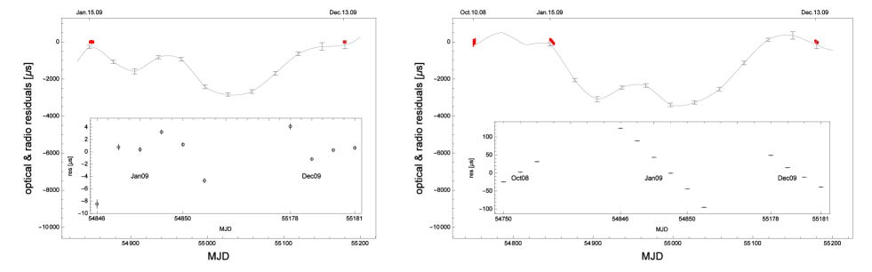
Figure 1: Residuals of optical and radio phase with respect to a BIM model. Left: best-fitting BIM to 2009 Iqueye data ($n=2.437$). Right: best-fitting BIM to 2008 - 2009 Aqueye and Iqueye data ($n=2.476$). Optical residuals are plotted as red data points clustered at the time of optical observations, while Jodrell Bank residuals (over the same interval of time) are represented by a gray line crossed by error bars at epoch dates of JBE. Insets: Zoom of average optical phase residuals during observation nights with 1$\sigma$ error bars. The scales of the y-axis in the insets are very different.

Our analysis leads to the following conclusions:

• The optical phase always leads the radio one. For three sets of observations, the time lapse between optical measurement and JBE reported radio phase (the latter refers to the center of the main pulse) was between 160 and 260$\mu$s (Germanà et al. 2012; Zampieri et al. 2014). Therefore, there is no evidence for any significant change in the delay between the three epochs. Accurate estimates of the X-ray-radio delay have been reported by Rots et al. (2004) (344$\pm$40 $\mu$s) and show that it does not change on a timescale of several years. No other difference between optical and radio outside the quoted interval of uncertainty has been found. We note that this delay is also consistent with other recent measurements performed in the optical band (e.g., Oosterbroek et al. 2006, 2008).

• A braking index law can reproduce the phase history during the studied 14-month period to within one turn with a narrow range of braking parameters, yet residuals with respect to such a description represent timing noise present on all wavebands and thus most likely reflect genuine variations in rotation of the Crab pulsar. This then motivates us to use JBE data for studying the long-term intrinsic rotation properties of the pulsar.

• The small residuals shown in the inset of lefthand part of Fig. 1 are real and should be considered as typical of short, daily timescale phase noise during a quiet glitch-less period of pulsar history. They are shown again in Fig. 2, together with polynomial fits through data points on the left, and frequency and frequency derivative residuals corresponding to these polynomials on the right. Thus, these data suggest “typical” frequency noise on a daily scale at the level of $\sim 10^{-8}s^{-1}$ and “typical” frequency derivative noise on a daily scale at the level of a few times $10^{-13}s^{-2}$. These estimates are in reasonable agreement with the difference in frequency and frequency derivative derived from optical and radio data (Zampieri et al. 2014) which are January 15. 2009: $f_{opt}-f_{radio}=-5.64\times 10^{-9}s^{-1}$, $\dot{f}_{opt}-\dot{f}_{radio}=1.55\times 10^{-14}s^{-2}$; and December 15. 2009: $f_{opt}-f_{radio}=-6.45\times 10^{-9}s^{-1}$, $\dot{f}_{opt}-\dot{f}_{radio}=-6.86\times 10^{-15}s^{-2}$.

2.1 Braking index model implementation

The braking index model implies that the phase $\varphi$ can be expressed as

$$\varphi(t)=c+a(1+bt)^{s},$$ (1)

where $c$ is an integration constant that can be used to adjust the initial phase, $a$ and $b$ are parameters that are related to the age and frequency of the pulsar at $t=0$, and $s=\frac{n-2}{n-1}$ is the braking parameter. The frequency and its derivative are then the following functions of time $f=\dot{\varphi}=sab(1+bt)^{s-1}$ and $\dot{f}=\ddot{\varphi}=s(s-1)ab^{2}(1+bt)^{s-2}$. The last equation leads to the familiar form of the braking index law:

$$\dot{f}=\left[b(s-1)\left(sab\right)^{\frac{1}{s-1}}\right]f^{\frac{s-2}{s-1}},$$ (2)

therefore $n=\frac{s-2}{s-1}$.

To compare our optical data with radio data as documented in JBE, we devised a numerical procedure that expresses the phase as the number of turns that the pulsar has made since the first pulse arrival time on May 15. 1988; i.e., $\phi(t)=0$ at MJD=47296.0000003712. More details are given in Appendix A.

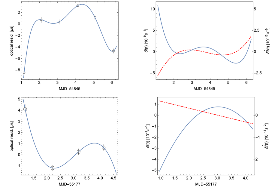
Figure 2: January (top) and December (bottom) 2009 optical residuals (Fig. 1) fitted to polynomials that reveal “typical” noise in pulsar frequency and frequency derivative, as shown on the right, in solid line for frequency residuals (left scale) and dashed for frequency derivative residuals (right scale).

3 Braking episodes

That the phase history of the Crab pulsar can be approximated by a BIM to within one turn during a 14-month period raises the question of how long such a description can go on? This idea can best be analyzed by using the publicly available JBE Crab pulsar ephemerides since 1988 because they represent the most complete and uniform description of Crab rotational history, which has been shown to be consistent with data in other wavebands. As a first step in finding periods during which the braking index may be sufficiently constant, we plot residuals of JBE-published frequency derivatives with respect to frequency derivatives predicted by a BIM with $s=\frac{n-2}{n-1}=1/3$ ($n=2.5$) and the parameters $a$ and $b$ in equation (1) chosen by a least squares fit minimizing residuals ${\dot{f}}_{res}={\dot{f}}_{JBE}-\dot{f}$. These residuals are shown in Fig. 3.

The graph clearly shows that on average, the $n=2.5$ braking index law describes the 26-year phase history reasonably well. However, large systematic changes in slope immediately after some (major) glitches signal that during such periods, the braking index must be different from the average value. Therefore, we divide the 26-year interval into ten subintervals, henceforth called episodes (see Fig. 3), each corresponding to periods characterized by the absence of pronounced changes in the braking index. We expect that the phase history during an episode can be largely approximated by a constant braking index law, as in the case of the interval of comparison of optical and radio data. At this stage in our discussion, the exact dates of the ten episodes are not yet well defined. In the next sections we show how they can be better constrained.

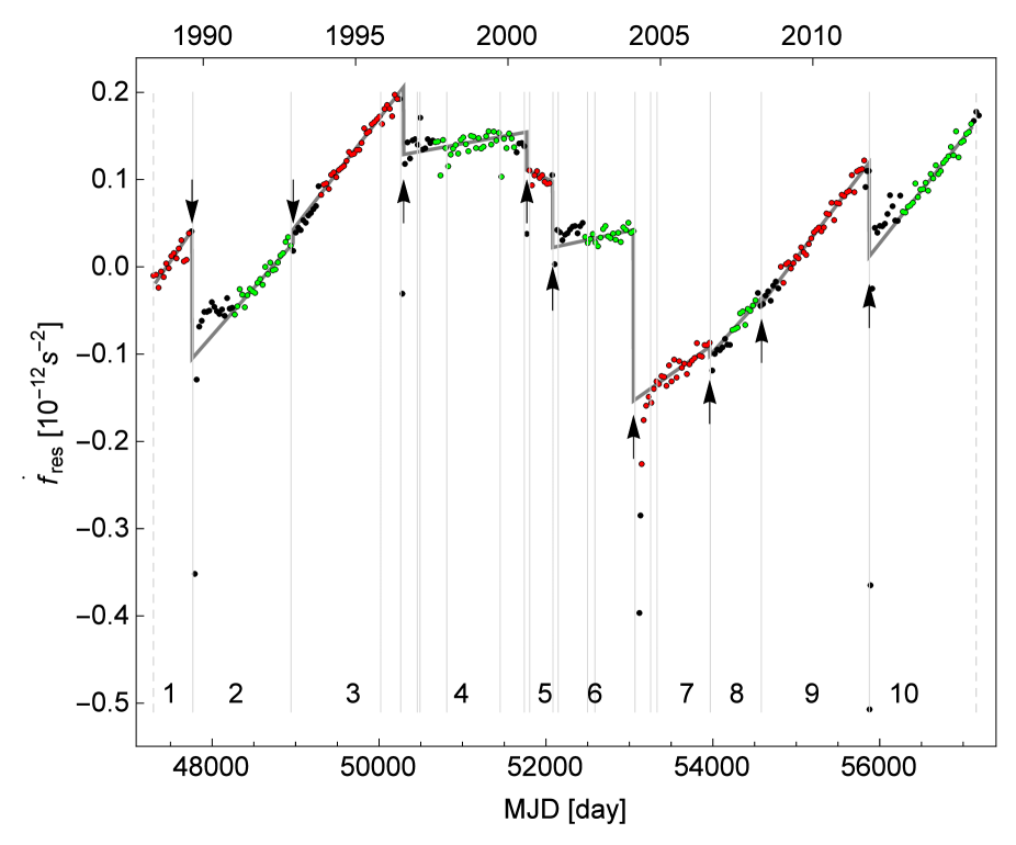
Figure 3: Residuals of JBE frequency derivatives with respect to a constant braking index law fit with $n=2.5$, calculated over the whole JBE interval (from 1988 May through 2015 June 15th). The vertical gray lines denote the occurrence of glitches as reported by Espinoza et al. (2011) and http://www.jb.man.ac.uk/$\sim$pulsar/crab.html (see Table 3). Nine arrows delimit chosen episodes and are placed at times when (major) glitches appear to change the braking index. The two dashed vertical lines mark the beginning and the end of the data set. The gray broken line indicates the second derivative of the continuous phase function defined in the text. Points used for the fit with the braking law model $\varphi_{j}(t)$ are displayed in red and green, while points in black are excluded from the fit, as explained in the text. Some post glitch residuals with the value below $-0.5\times 10^{-12}s^{-2}$ go beyond the scale and are not shown.

To be able to properly categorize a glitch as a discontinuous change in frequency and frequency derivative, one would need densely distributed high resolution optical data from such an event. Unfortunately, they are not available yet. To get an idea of how the spin-down behaves before and after the glitch event, we used the public available data (Lyne, Pritchard, & Graham-Smith (1993) and http://www.jb.man.ac.uk/$\sim$pulsar/crab.html) and built the phase history since May 15, 1988, assuming that the phase prediction by the suggested third-degree polynomial is accurate to a (small) fraction of a period during each ephemerides epoch and that the phase is continuous between successive periods. We built up a table of pulsar’s integer radio phase at the exact Julian dates of pulse arrival times given by JBE. This table T is a table of entries of main pulse arrival times and integer number of turns the pulsar has made from the starting date. This table is broken into ten episodes according to boundaries shown in Fig. 3 and determined as explained below (see also Appendix A).

Inside each episode we seek a braking index law $\varphi_{j}(t)$ in the same form as in Eq. 1 with $s_{j}$ as an additional fitting parameter. Our goal is to obtain the $s_{j}$ for the braking law that fits the particular episode, in such a way that it gives the smallest residuals over the whole episode. It turns out that this goal can only be achieved by using data in the apparently quiet part of the episode, disregarding scattered data immediately after the glitch at the beginning of the episode. Data points whose phase is not considered in the fit are colored black in Fig. 3 (we comment on this choice below). In this way we obtain local fits $\varphi_{j}(t)=c_{j}+a_{j}(1+b_{j}t)^{s_{j}}$, valid on complete intervals of episodes $\{T^{b}_{j},T^{b}_{j+1}\}$, where $T^{b}$ is the starting MJD for each episode.

These local fits are joined into a continuous curve $\Phi(t)$ by choosing $c_{j+1}$ in such a way that $\varphi_{j+1}(T^{b}_{j+1})=\varphi_{j}(T^{b}_{j+1})$. Residuals of the fit ($R(t)={\bf T}-\Phi(t)$) are shown in Fig. 4 at all data points, and the parameters of $\varphi_{j}(t)$, expressed as a Taylor series expansion of Eq. (1), are given in Table 1. When varying the parameters within the reported errors, the solution deviates from the best fits by less than 0.001 turn. The fits to those residuals, discussed in the next section, are also shown as blue and cyan curves on top of the R(t) dots in Fig. 4 (dots also include black data points in Fig. 3).

j	$T^{b}_{j}\ [MJD]$	$\psi_{j}[10^{9}]$	$\delta\psi_{j}$	$\nu_{j}\ [s^{-1}]$	$\delta\nu$	$\dot{\nu}_{j}\ [10^{-10}s^{-2}]$	$\delta\dot{\nu}$	$\ddot{\nu}_{j}\ [10^{-20}s^{-3}]$	$\delta\ddot{\nu}$	$\dddot{\nu}_{j}\ [10^{-31}s^{-4}]$	$n_{j}$	$\delta n$
1	47327	0.080308783914	1.	29.98335828167	3.	-3.785953271	14.	1.223496	12.	-6.3	2.559365	24.
2	47759	1.199168006987	1.	29.96923749017	1.	-3.782862267	1.8	1.189028	0.52	-5.9	2.490158	1.1
3	48971	4.335378859396	1.	29.92968949582	0.9	-3.770288188	1.5	1.200702	0.40	-6.1	2.528066	0.85
4	50294	7.754097684269	1.	29.88667114924	0.8	-3.757375987	1.2	1.071861	0.29	-4.7	2.269065	0.61
5	51771	11.564963729546	1.	29.83880913666	4.	-3.744175564	28.	0.9995258	32.	-4.1	2.127468	67.
6	52080	12.361454906619	1.	29.82881752567	1.	-3.742269975	2.9	1.068559	1.0	-4.7	2.275959	2.2
7	53049	14.857460749680	1.	29.79752549720	1.	-3.735298384	3.2	1.119064	1.2	-5.3	2.389927	2.6
8	53962	17.206823673457	1.	29.76809511938	2.	-3.726586977	6.9	1.160253	3.9	-5.7	2.487030	8.3
9	54584	18.806047084704	1.	29.74808502226	0.9	-3.720427194	1.6	1.180117	0.43	-6.0	2.536288	0.93
10	55874	22.119341521240	1.	29.70669287202	0.9	-3.708385813	1.8	1.169154	0.51	-5.9	2.525551	1.1

Table 1: Parameters of local fits for different j episodes, expressed in the form of a Taylor series of the form $\varphi_{j}(t)=\psi_{j}+\nu_{j}t+\frac{1}{2}\dot{\nu}_{j}t^{2}+\frac{1}{6}\ddot{\nu}_{j}t^{3}+\frac{1}{24}\dddot{\nu}_{j}t^{4}$ where the coefficients are constrained to fit the braking index law: i.e., this expression is a Taylor series expansion of Eq. (1). Quoted errors refer to the last reported digit. Time in the argument of $\varphi_{j}$ starts at 00 UT of the appropriate $T^{b}_{j}$. The last two columns give the corresponding values of the braking index and its error.

Residuals in Fig. 4 show that, during each episode, it is possible to find a local braking law with respect to which $R\left(t\right)$ is never more than a few turns, even if the pulsar makes billions of turns during the same period. It must be emphasized that residuals that are as small as those shown in Fig. 4 can only be obtained by fitting the phase on different episodes T_j with markedly different braking law indices, varying from $\sim 2.1$ to $\sim 2.6$.

As already mentioned in the discussion of fitting optical data (see Fig. 1), the precise value of the braking index on the episode may depend on the selection of data points after the glitch. Looking at Fig. 3, different choices for the black, green, and red points can possibly be made. However, the requirement that phase residuals be as small as only a few turns very clearly narrows down an already narrow range of acceptable values of the braking index for each episode. Finally, since $\Phi(t)$ is a continuous function, the residuals $R(t)$ must also be continuous at the boundaries between episodes. This requirement narrows down the dates of boundaries between episodes to values $T^{b}_{j}$ as listed in Table 1.

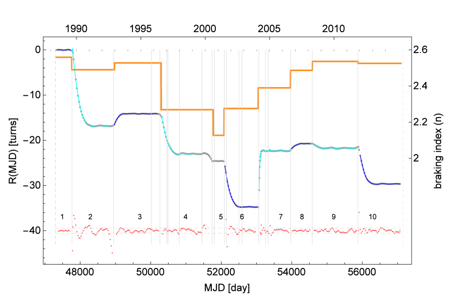
Figure 4: JBE phase residuals $R(t)$ with respect to local fits $\varphi_{j}(t)$ calculated for the 10 chosen episodes (see Fig. 3). Gray vertical lines are plotted at the dates of reported glitches (Espinoza et al. 2011). The braking index during episodes is shown in orange. Sinusoidal fits to residuals, discussed below, are shown in blue and cyan to distinguish episodes. Red points at the bottom show ten times the difference between $R(t)$ and sinusoidal fits $R_{j}(t)$ at data points; the horizontal dashed lines bracket these final residuals with their standard deviation of 0.057 turns; the distribution of final residuals has wider wings than a Gaussian.

4 The rotational phase history of the Crab pulsar

It is remarkable that the evolution of the rotational phase of the Crab pulsar can be split into two parts: a regular phase $\Phi(t)$ consisting of a constant braking index during a given episode, but different for each episode, and a small residual phase $R(t)$ that, during all this time, wanders by no more than 35 turns, to be compared with the $\sim 2.5\times 10^{10}$ turns the pulsar has made during the 9800 days covered by the JBE (see Fig. 4).

According to the dates reported in JBE and in Espinoza et al. (2014), jumps in braking index are clearly related to large glitches (see Table A1), while small glitches do not leave a notable imprint on the curve $R(t)$. To recover the significance of small glitches from JBE, we calculated the second derivative of the function $R_{s}(t)$, which is constructed as a differentiable function from tabular values of $R(t)$ by cubic spline interpolation. The result is shown in Fig. 5 (left panel). In this representation, small glitches, except possibly a few (n. 10, 11, 13), show up as spikes barely above the general noise in ${\ddot{R}}_{s}(t)$. Only nine glitches (n. 6, 7, 9, 14, 16, 20, 23, 24, 25) show second-derivative ${\ddot{R}}_{s}(t)$ beyond $2\times 10^{-14}s^{-2}$, which is smaller than the second derivative of optical phase residuals derived from the January 2009 data (${\ddot{R}}_{Jan}\approx 10^{-13}s^{-2}$ see Fig. 2). All of them are clearly related to a change in the braking index (Fig. 4). The righthand panel of Fig. 5 shows phase residuals $R_{s}(t),$ together with phase residuals calculated as suggested by explanatory notes of JBE. Breaks (a few thousands of a turn) between the ephemerides dates, occur because the suggested expression for calculating the phase increment,

$$\varphi(t)=\varphi(t_{0})+\frac{1}{P}(t-t_{0})-\frac{1}{2}\frac{\dot{P}}{P^{2}}(t-t_{0})^{2}+\frac{1}{3}\frac{{\dot{P}}^{2}}{P^{3}}(t-t_{0})^{3},$$ (3)

(P is the nominal period) does not yield an exact integer number of turns between two entries in Table $\bf T$. We suspect that the actual pulsar phase noise variation (Wong, Backer, & Lyne 2001) is the dominant cause for those phase residuals breaks. The truncated Taylor series in Eq. (3) is probably not sufficient to take complete account of phase noise variation. Intrinsic timing noise has also been confirmed by optical observations (Fig. 2), and according to Zampieri et al. (2014), the difference in frequency derivative obtained from radio ephemerides and from optical observations is consistent with the difference between the red and blue curve in the righthand panel of Fig. 5.

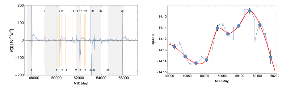
Figure 5: Left: Second time derivative of the residual phase $R_{s}(t)$, a third-order spline fit through phase residuals from Table $\bf{T}$. The orange vertical lines are drawn at dates of reported glitches and labeled according to Table 3. Episodes are shaded intermittently as light gray and white. Right: Phase residuals as a function of time for a short interval during episode 3. The red line shows $R_{s}(t)$, while the blue line is calculated as suggested by explanatory notes of JBE (see text for details). Error bars show JBE quoted arrival-time uncertainties.

The curves of residuals in Fig. 4 all have a characteristic shape. It is customary to express functions describing sets of data with a linear combination of a certain Hilbert space basis (eigenvectors) and natural to choose such a basis so that the concrete experimental result can be described by the fewest components. Having tried different possibilities (including the widely used combination of sinusoids $+$ decaying exponentials), we find that the residuals can be described by only two complex Fourier components:

$$R_{j}(t)=\Psi_{j}+A_{j}e^{-\lambda_{j}(t-T^{b}_{j})}\sin\left(\omega_{j}(t-T^{b}_{j})+\delta_{j}\right)$$ (4)

$$+{\overline{A}}_{j}e^{-{\overline{\lambda}}_{j}(t-T^{b}_{j})}\sin\left({\overline{\omega}}_{j}(t-T^{b}_{j})+\overline{\delta}_{j}\right).$$

We believe that this mathematical approach leads to a simpler description of pulsar noise. The coefficients are given in Table 2 and are sufficient to produce a fit of $R(t)$ without systematic trends in the residuals, as shown in gray at the bottom of Fig. 4. The standard deviation of the distribution of phase residuals is 0.057. It can be compared with the standard deviation of the set of fractional phase residuals between ephemerides epochs, which is 0.063. The declared arrival-time uncertainty in JBE is 0.01 or 300$\mu$s. The details of these fits, together with some other pertinent information, are shown in Fig. 6.

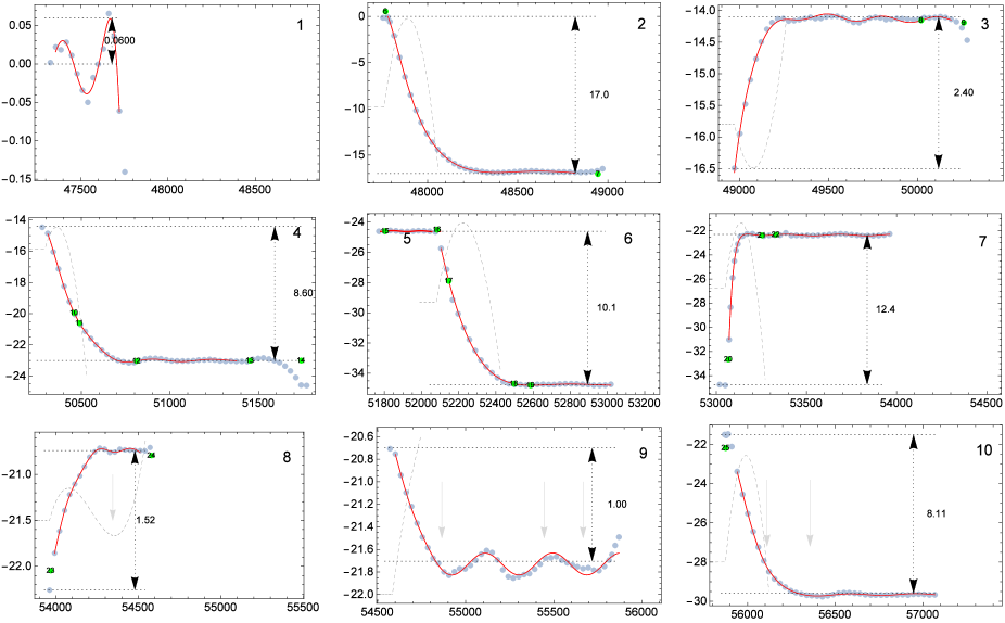
Figure 6: Sinusoidal phase functions $R_{j}(t)$ (red lines) that fit the JBE phase residuals (blue points) for episodes from $j$ = 1 to 10 (the short episode 5 is included in the graph showing episode 6). Time on the abscissa is in MJD, and the scale is the same for all episodes. Green dots are numbered as in Espinoza et al. (2011) at dates of published glitches with the ordinate as calculated from $R_{j}(t)$. Ordinate scales are different and adjusted to different amplitudes of oscillations. Each panel shows data of the complete episode and includes the first point of the next episode. The difference between horizontal dotted lines represents a measure of the strength of the perturbation $R_{j}(t)$ caused by the glitch. Dashed gray curves are the plots of $\varphi_{j}(t)-\varphi_{j-1}(t)$, to show the difference of phases between two contiguous episodes. Gray arrows point to dates of the $>100$ MeV X-ray flares detected by Fermi (Abdo et al. 2011; Ojiha et al. 2013; Bühler et al. 2012) and AGILE (Tavani et al. 2011; Striani et al. 2013).

j	$\Psi$	$\omega\left[{\rm day}^{-1}\right]$	$\lambda\left[{\rm day}^{-1}\right]$	$A$	$\delta$	$\overline{\omega}\left[{\rm day}^{-1}\right]$	$\overline{\lambda}\left[{\rm day}^{-1}\right]$	$\overline{A}$	$\overline{\delta}$
1	-0.004	0.0345	-0.0209	0.0000254	-3.47	0.0236	0	0.034	-0.0955
2	-16.91	0.0010	0.0113	177.00	0.100	0.0091	0	0.153	-0.0392
3	-14.15	0.0010	0.0072	8.63	-0.282	0.0206	0	0.047	-2.9822
4	-22.98	0.0054	0.0092	14.4	0.621	0.0187	0.0018	0.320	2.7275
6	36.72	0.0037	0.0018	12.7	-2.46	0.0008	0	73.50	-2.3370
7	-22.35	0.0010	0.0321	217.	-0.103	0.0213	0	0.066	0.5691
8	-20.78	0.0068	0.0075	1.36	-1.86	0.0306	0	0.029	-1.0713
9	-21.72	0.0072	0.0131	1.68	0.73	0.0163	0	0.098	-0.709
10	-29.65	0.0059	0.0102	16.1	0.48	0.0166	0	0.046	2.45

Table 2: Coefficients of the fitting function $R_{j}(t)$ in Eq. 2

The ansatz in Eq. 4 is purely mathematical and is an almost satisfactory description of phase residuals $R(t)$. A posteriori, we note that the first sinusoid has very low values of $\omega$ so is essentially a decaying component, while in all episodes but one, the second sinusoid is not damped.

It should be understood that glitches may not be modeled exactly by our analysis because the time resolution of JBE data is not sufficient to describe the exponential decay of a glitch that lasts a few days (Wong, Backer, & Lyne 2001). However, because of all that has been said, the JBE data are reliable as to the global phase behaviour and on timescales longer than about a month. In this respect, the decaying component at the beginning of several episodes resembles the usual after-glitch recovery behavior frequently modeled in the literature through a single-parameter exponential (e.g., Lyne et al. 2015, with a characteristic timescale of 320 days).

Figures 4 and 6 clearly illustrate the meaning of the split of the phase behavior into the braking index part $\Phi(t)$ and residuals $R(t)$. It is quite clear that toward the end of an episode, residuals relax to the perfect braking law solution and eventually oscillate for years by only a very small fraction of a turn. On the other hand, as hinted in Fig. 6, the braking-law part of an episode ($\varphi_{j}(t)$) generally differs quite considerably from the braking law of the previous episode ($\varphi_{j-1}(t)$). In fact, if the difference $\varphi_{j}(t)-\varphi_{j-1}(t)$ was plotted to the end of episodes, it would reach values several tens or a hundred times the value $\Delta N$. An exception is the short episode 8, which follows a relatively weak glitch. For this episode R(t) and $\varphi_{j}(t)-\varphi_{j-1}(t)$ are comparable, and therefore, the split between the braking index part and residuals is not as clear cut. Figure 6 also confirms that, within limits allowed by the time resolution of available data, the breaks between episodes occur on the dates of reported glitches. It appears plausible to classify glitches into two groups: those for which the change in the phase $\Phi(t)$ dominates residuals $R(t)$ by many factors of ten (6, 7, 9, 16, 20, 23, 24, 25) and those where the integral change in $\varphi_{j}(t)-\varphi_{j-1}(t)$ is comparable or insignificant with respect to the amplitude of $R(t)$ (all other glitches beyond #6).

5 Discussion and conclusions

Our analysis shows that the phase evolution of the Crab pulsar can be described as a series of constant braking-law episodes, with the braking index changing abruptly after each episode in the range of values between 2.1 and 2.6. Phase residuals with respect to such a smooth phase description amount to only a few turns in $\sim 10^{9}$ turns executed during an episode. The split between the smooth braking-law-dominated part and residuals is not mathematically unique, but requirements that phase residuals be as small as only a few turns and that the phase between ephemerides epochs clearly converges to the characteristic braking index solution of the episode narrow the choice of braking index parameters.

A similar conclusion concerning the behavior of the braking index has been recently obtained by Lyne et al. (2015) from an independent analysis of 45 years of radio data on the rotational history of the Crab pulsar. Results obtained from a fit with a single Taylor series returns a behavior of $f$ and $\dot{f}$ (their Figures 1 and 2) very similar to the one shown in Figure 3 (with a best fitting $n=2.34$). Variations in the braking index in the period between 1996 and 2006, characterized by a high concentration of glitches, were also noted by Lyne et al. (2015). While they consider it a weak, unexplained effect on the background of the previous rotational history (described by a simple slowdown with braking index 2.519(2)), we offer here a different interpretation that can account for the overall timing irregularities of the Crab pulsar.

According to our interpretation, glitches and abrupt changes in the braking mechanism may be part of the same physical process that also drives semi-periodic timing noise between glitches (Fig. 4). In fact, JBE data provide an interesting correlation of the braking index and dispersion measure. Namely, the dispersion measure (as listed in JBE) follows the braking index with a time delay of 1100${}^{+450}_{-250}$ days as shown in Fig. 7.

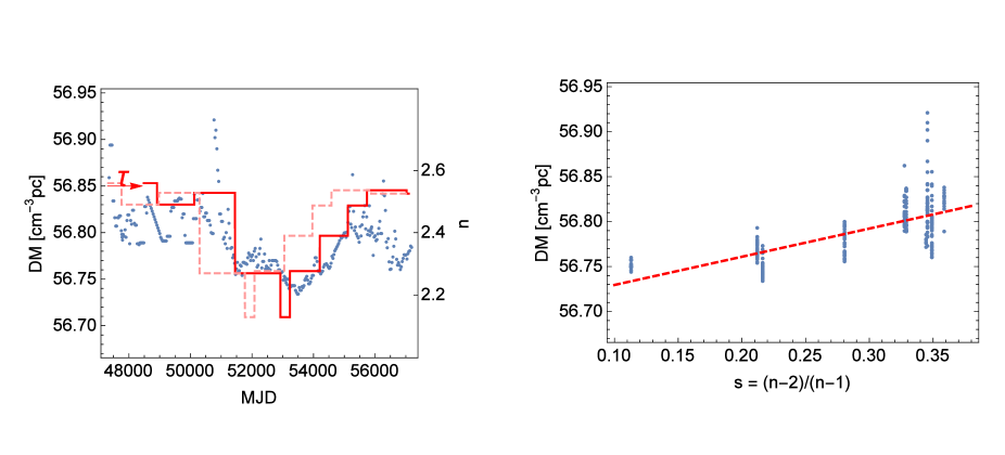
Figure 7: a) Left: dispersion measure $DM(t)$ (blue dots), braking index $n(t-\tau)$ for $\tau=1100$ days (continuous red line). The dashed red line shows $n(t)$. b) Right: correlation between braking index ($n$) and dispersion measure $DM$. The correlation coefficient is 0.7.

The delayed response of dispersion measure to the value of braking index lends support to the idea of Anderson & Itoh (1975) that change of the braking index has to do with a pulsar-wind-driving torque and is also consistent with the idea that eddy currents threading the pulsar nebula ionize it and thus inject varying amounts of free electrons.

From this new perspective, glitches, timing noise, changes in braking torque, and dispersion measure appear to be part of a common mechanism that jumps between different braking modes. Distinctly long timescales of timing noise oscillations suggest that the mechanism can hardly be connected to phenomena occurring within the pulsar. It appears plausible that the “instantaneous” change in braking torque is caused by some instability, which varies the configuration of the external electromagnetic field and currents in the nebular plasma through which the pulsar interacts with its nebula. Such an interaction is needed in order to understand the acceleration and energizing mechanisms of the pulsar nebula (Trimble 1968; Weyler & Panagia 1978), such as the highly dynamical flow of relativistic particles in the form of equatorial wind and polar jets, as seen in Hubble Space Telescope and Chandra images (Hester et al. 2002).

The possible occurrence of plasma instabilities causing “instantaneous” changes in the braking mechanism is expected to produce observable changes in radiation from the Crab nebula. It is tempting to consider the possibility (Cerutti et al. 2014) that plasma instabilities occurring through magnetic field line reconnection drive the recently observed gamma ray flares (Abdo et al. 2011; Tavani et al. 2011; Ojiha et al. 2013; Striani et al. 2013; Bühler et al. 2012). Arrows in Fig. 6 point to instants when the six observed flares occurred in the Crab nebula. The same mechanism, which also appears to be acting in the solar corona to produce gamma ray flares (Ajello et al. 2014), may be able to provide a sudden short release of braking torque by disconnecting the magnetic field lines from the pulsar from those threading the nebular plasma. The same mechanism may also be responsible for sharp increases in dispersion measure (Fig. 7, left) by emitting highly energetic particles into the neutral nebula, thus ionizing it.

The back reaction of plasma instabilities on the pulsar, possibly associated to these flares, has not been studied yet, but it does not seem to be simultaneous with the occurrence of the flare (Weisskopf et al. 2013; Zampieri et al. 2013). In view of the delayed correlation between dispersion measure and braking index, this appears understandable – perturbations caused by magnetic reconnection travel long distances before reaching the pulsar or before permeating the nebula. Nevertheless, the interflare time inferred from numerical simulations (hundreds of days) (Mignone et al. 2013; Porth, Komissarov, & Keppens 2014; Cerutti et al. 2014) appears to be broadly consistent with the timescales observed in oscillations of JBE phase residuals. It is quite remarkable that the occurrence of the reported gamma-ray flares is also consistent with such a timescale.

Our ultra-fast optical observations of the Crab pulsar with Aqueye and Iqueye stimulated the line of research presented here. Future simultaneous radio and optical timing measurements, as well as optical imaging and gamma-ray observations, will be crucial for revealing the source of the braking mechanism, in particular if it is located in the external electromagnetic field through which the pulsar interacts with the surrounding plasma, as suggested by our results.

Appendix A Crab phase data

We construct the decadal timing solution of the Crab pulsar as a series of pairs $\bf{T}_{j}=\{\rm{MJD}_{j}+(1/86400)\rm{TOA}_{j},z_{j}\}$, where $\rm{MJD}_{j}$ is the mean Julian date of the $j$-th entry of JB ephemerides, $\rm{TOA}_{j}$ is the first arrival time of the pulse at $\rm{MJD}_{j}$ (the t_JPL entry in JBE), and $z_{j}$ is the integer number of turns the pulsar has made from the starting date May 15, 1988 (MJD₁=47296). Integers $z_{j}$ are calculated by summing the integer number of turns N_j that the pulsar has made between MJD_j-1 and MJD_j ($z_{j}=\sum{}^{j}_{k=1}N_{k}$). N_k is calculated using the JB published values of frequency and frequency derivative. Using the formula suggested by explanatory notes to JBE, we calculate it as follows.

Let $\Delta t=43200\left({\bf T}_{j}-{\bf T}_{j-1}\right)$, and let $\nu_{j}$ and ${\dot{\nu}}_{j}$ be the frequency and frequency derivative listed at the j-th ephemerides entry in JBE. Define $P_{j}=1/\nu_{j}$ and ${\dot{P}}_{j}=-{\dot{\nu}_{j}}{\nu_{j}}^{-2}$, then $\Delta N=\left(\frac{1}{P_{i-1}}+\frac{1}{P_{i}}\right)\Delta t-\left(\frac{\dot{P}_{j-1}}{{P_{j-1}}^{2}}-\frac{\dot{P}_{j}}{{P_{j}}^{2}}\right)\frac{\Delta t^{2}}{2}+\left(\frac{{\dot{P}_{j-1}}^{2}}{{P_{j-1}}^{3}}+\frac{{\dot{P}_{j}}^{2}}{{P_{j}}^{3}}\right)\frac{\Delta t^{3}}{3}$ and $N_{j}=$IntegerPart$[\Delta N]$. The evaluation of $\Delta N$ in most cases yields an integer, as it should. However, in 25 cases, almost all of them occurring at the time of a glitch, the calculated number of turns between successive TOA’s has a fractional part that is inconsistent with the quoted TOA accuracy. The fractional phase errors are shown in Fig. 8.

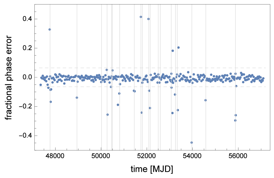
Figure 8: Fractional part of calculated number of turns between successive TOAs’ fractional phase error. Vertical lines denote the dates of reported glitches, starting from glitch no. 5 in Table 3. Horizontal dashed lines are at $\pm 0.062$, the variance of the (wide winged) phase error distribution.

no	glitch	episode	$T^{b}$	$\delta f/f$
	[MJD]	no.	[MJD]	[$10^{-9}$]
1	40491.8			7.2
2	41161.98			1.9
3	41250.32			2.1
4	42447.26			35.7
5	46663.69			6.0
		1	47327
6	47767.504	2	47759	81
7	48945.6	3	48971	4.2
8	50020.04			2.1
9	50260.031	4	50294	31.9
10	50458.94			6.1
11	50489.7			0.8
12	50812.59			6.2
13	51452.02			6.8
14	51740.656	5	51771	25.1
15	51804.75			3.5
16	52084.072	6	52080	22.6
17	52146.758			8.9
18	52498.257			3.4
19	52587.2			1.7
20	53067.078	7	53049	214
21	53254.109			4.9
22	53331.17			2.8
23	53970.19	8	53962	21.8
24	54580.38	9	54584	4.7
25	55875.5	10	55874	49.2

Table 3: Numbers and dates of glitches (from Espinoza et al. (2011)). The MJD episode is the starting date of the episode as listed in Table 1, and the last column quotes reported frequency jumps during the glitch.

Table A.1 lists all glitches reported in Espinoza et al. (2011) (http://www.jb.man.ac.uk/pulsar/glitches.html) and the starting dates of episodes 2 to 10.