Cosmic Acceleration From Matter–Curvature Coupling

Abstract

We consider $f\left({R,T}\right)$ modified theory of gravity in which, in general, the gravitational Lagrangian is given by an arbitrary function of the Ricci scalar and the trace of the energy–momentum tensor. We indicate that in this type of the theory, the coupling energy–momentum tensor is not conserved. However, we mainly focus on a particular model that matter is minimally coupled to the geometry in the metric formalism and wherein, its coupling energy–momentum tensor is also conserved. We obtain the corresponding Raychaudhuri dynamical equation that presents the evolution of the kinematic quantities. Then for the chosen model, we derive the behavior of the deceleration parameter, and show that the coupling term can lead to an acceleration phase after the matter dominated phase. On the other hand, the curvature of the universe corresponds with the deviation from parallelism in the geodesic motion. Thus, we also scrutinize the motion of the free test particles on their geodesics, and derive the geodesic deviation equation in this modified theory to study the accelerating universe within the spatially flat FLRW background. Actually, this equation gives the relative accelerations of adjacent particles as a measurable physical quantity, and provides an elegant tool to investigate the timelike and the null structures of spacetime geometries. Then, through the null deviation vector, we find the observer area–distance as a function of the redshift for the chosen model, and compare the results with the corresponding results obtained in the literature.

PACS numbers: 04.50.Kd; 95.36.+x; 98.80.-k; 04.20.-q; 04.20.Cv
Keywords: $f(R,T)$ Modified Gravity; Cosmic Acceleration Phase; Geodesic Deviation Equation.

1 Introduction

The measurements of type Ia supernovae luminosity distances indicate that the universe is currently undergoing an accelerated expansion [1]–[4]. The cause of this late time acceleration has been one of the most challenging problems of modern cosmology. Such an acceleration requires, in general, some components of negative pressure, with the equation of state parameter, $w$, less than $-1/3$, to make an acceleration for the universe. Several mechanisms, that are considered to be responsible for this expansion, have been proposed, namely in particular: the $\Lambda$CDM model, dark energy models and modified gravities. In the $\Lambda$CDM model (e.g., Refs. [5, 6]), around $31\%$ of the mass–energy density of the universe is made of the barionic and dark matter, and the rest is constituted by the cosmological constant [7, 8]. Actually, the cosmological constant is the simplest candidate which corresponds to the value of $w=-1$, however, the value of the observed cosmological constant is less than the Planck scale by a factor of $120$ orders of magnitude. This problem, that is related to the non–comparability of the value of dark energy density with the field theoretical vacuum energy, is called the cosmological constant problem, see, e.g., Refs. [6, 9]–[13].

Another approach has been generalized by considering a source term, with an equation of state parameter less than $-1/3$, that is known as dark energy, see, e.g., Refs. [14]–[20]. However, the nature of dark energy is still unknown and actually, the nature of both the dark matter and dark energy are one of the most important issues in physics. In this approach, the observed cosmological evidences imply on the existence of these components of the cosmic energy budget, and even indicate that around $95\%$ of the universe is composed by the dark matter and dark energy. Some candidates for the dark matter (e.g., neutralinos and axions) and dark energy (e.g., quintessence) have been considered, although no direct detection has been reported until now. Also, various scalar field models of dark energy have been studied in the literature, e.g., Refs. [21]–[23].

On the other hand, the late time acceleration can be caused by purely gravitational effects, i.e. one may consider modifying the gravitational theory, see, e.g., Refs. [24]–[28]. For instance, $f(R)$ gravities (as the simplest family of the higher–order gravities) have been based on replacing the scalar curvature $R$ in the Einstein–Hilbert action with an arbitrary differentiable function of it. In this regard, and as an example, it has been shown in Refs. [29, 30] that by adding a term of $1/R$ to $R$, when the inverse curvature term dominates, one typically expects that the universe expands with the desired late time acceleration, however, this model suffers from a number of problems such as matter instability, see, e.g., Ref. [31]. As an another interesting example, it has been illustrated in Ref. [32] that with a $5$–dimensional $f(R)$ in the brane world scenario (that converts to a scalar–tensor type theory with a scalar field), an accelerated expanding universe emerges for a suitable choice of the function $f$. However, $f(R)$ theories are somehow equivalent to the scalar–tensor theories, in particular, to the specific type, namely the Brans–Dicke theory, see, e.g., Ref. [33, 34] and references therein. Actually, it has been claimed [34] that these theories are effectively have the same phenomenology in most applications in cosmology and astrophysics. For review on the generalized gravitational theories, see, e.g., Refs. [35]–[42].

In this work, we propose to probe the cosmological considerations of another type of modified gravity theories, namely $f(R,T)$ gravity, see, e.g., Refs. [43]–[53]. Theory of $f(R,T)$ gravity generalizes theories of gravity by a priori incorporation of the trace of dustlike matter energy–momentum tensor ($T$) in addition to the Ricci scalar into the Lagrangian of geometry. The reason for the a priori dependence on $T$ may be the inductions arising from some exotic imperfect fluids and/or quantum effects (e.g., the conformal anomaly), and anyway, the $f(R,T)$ gravity model depends on a source term, while somehow represents the variation of the energy–momentum tensor with respect to the metric. In another word, the a priori appearance of the matter in an unusual coupling with the curvature may also have some relations with the known issues such as, geometrical curvature induction of matter, a geometrical description of physical forces, and a geometrical origin for the matter content of the universe, see, e.g., Refs. [55, 56] and references therein. In this respect, whilst we first derive the necessary equations for any arbitrary function of $f(R,T)$, the main purpose of the work is to concentrate on a simplest and yet the most plausible case of $f(R,T)$ gravity wherein the matter is also minimally coupled to the curvature. Then, we obtain the state parameter and the scale factor for this model in the matter dominated and the acceleration phase of the universe. And mainly, we investigate the effect of the cosmic matter and its coupling with geometry in the evolution of the universe in addition to the effect of pure geometry.

On the other side, to make our investigations for the acceleration of the universe more instructive, we also scrutinize the motion of the free test particles on their geodesics. In this regard, in the context of relativistic gravitational theories, the curvature of the spacetime plays a fundamental role instead of forces acting in the Newtonian theory. On the other hand, the Einstein field equations tell us how the curvature depends on the matter sources, where one can attain the effects of the curvature in a spacetime through the geodesic deviation equation (GDE) via derivation of the behavior of timelike, null and spacelike geodesics, as have been performed in Refs. [57]–[59]. Indeed, the GDE gives the relative acceleration of two adjacent geodesics as a measurable physical quantity, or a way that one can measure the curvature of spacetime (analogous to the Lorentz force law), see Refs. [60, 61]. Moreover, it specifies the tendency of free falling particles to recede or approach to each other while moving under the influence of a varying gravitational field, i.e. there exist internal effective tidal forces that cause the trajectories of free particles to bend away or towards each other. Also, the GDE provides a very elegant way of understanding the structure of a spacetime and renders an invariant procedure of characterizing the nature of gravitational forces [62]. And more interesting, this equation contains many important results of standard cosmology such as the Raychaudhuri dynamical equation [63], the observer area–distance (e.g., the Mattig relation for the dust case [64]), and how perturbations influence the kinematics of null geodesics in resulting gravitational–lensing effects [65] and references therein. In this respect, as far as we are concerned, the GDE was studied within the spatially flat Friedmann–Lemaître–Robertson–Walker (FLRW) spacetime geometries for general relativity plus cosmological term in Ref. [59]. And thereafter, it has been probed in the context of modified gravity theories, namely, the Palatini formalism of $f(R)$ [66], the metric $f(R)$ gravity [67, 68], arbitrary matter–curvature coupling theories [69], a well–known class of $f(R)$ theory [70], and $f(T)$ gravity (where in this theory, $T$ is the torsion scalar arising from the torsion tensor) [71].

The present work is organized as follows. The field equations and the cosmological aspects of the modified $f(R,T)$ gravity are derived in Sect. 2, in where we specify the generalized form of the Raychaudhuri dynamical equation that gives the evolution of the kinematic quantities in the framework of modified $f(R,T)$ theory. The minimal coupling models are considered in Sect. 3, wherein the matter dominated and the acceleration epochs are discussed in a more detail for a particular model, as a simple and plausible case of the minimal coupling models. Sect. 4 is devoted to: obtain the GDE in this type of theory for timelike and null geodesics within the spatially flat FLRW background, get a particular case of the Raychaudhuri dynamical equation, and to derive an useful relation measuring the observer area–distance as a function of the redshift. Then in the same section, we attain the results for the $\Lambda$CDM model and the particular minimal coupling model, and compare them with each other and also with the corresponding results of the Hu–Sawicki models [72] of $f(R)$ theories obtained in Ref. [70] and $f(T)$ gravity attained in Ref. [71]. Finally in Sect. 5, we present the conclusions. Through the work, we use the sign convention $({-,+,+,+})$ and geometrical units with $c=1$.

2 Modified Field Equations

In this section, we obtain the field equations and some corresponding dynamical parameters of $f(R,T)$ modified gravity in four dimensional spacetime. The action is simply written in the form

$$S=\int{{d^{4}}x\sqrt{-g}\left[{\frac{1}{{2\kappa}}f\left({R,T}\right)+{L_{m}}}\right]},$$ (1)

where $\kappa\equiv 8\pi G$, $g$ is the determinant of the metric and ${L_{m}}$ is the matter Lagrangian density, though for simplicity and plausibly for our purposes, we assume it to be only of the form of dustlike (non–relativistic) one. Also, the energy–momentum tensor is usually defined as

$$T_{\mu\nu}^{[m]}=-\frac{2}{{\sqrt{-g}}}\frac{{\delta({\sqrt{-g}{L_{m}}})}}{{\delta{g^{\mu\nu}}}},$$ (2)

where the lower case Greek indices run from zero to three and the index $m$ stands for the dustlike matter. Variation of the action with respect to the metric tensor gives the field equations

$${f_{R}}{R_{\mu\nu}}-\frac{f}{2}{g_{\mu\nu}}+\left({g_{\mu\nu}{\Box}}-{\nabla_{\mu}}{\nabla_{\nu}}\right){f_{R}}=\left({\kappa+{f_{T}}}\right)T_{\mu\nu}^{[m]},$$ (3)

where $\Box\equiv{\nabla_{\mu}}{\nabla^{\mu}}$ and we have defined the following functions for the derivative of the function $f(R,T)$ with respect to its arguments, i.e.

$${f_{R}}\equiv\frac{{\partial f(R,T)}}{{\partial R}}\qquad\qquad\quad{\rm and}\qquad\qquad\quad{f_{T}}\equiv\frac{{\partial f(R,T)}}{{\partial T}}.$$ (4)

By contracting the field equations (3), we attain the scalar equation

$${f_{R}}R-2f+3\,{\Box}{f_{R}}=\left({\kappa+{f_{T}}}\right)T.$$ (5)

It is more instructive to write the field equations in the form of the Einstein equations with an effective energy–momentum tensor, as

$${G_{\mu\nu}}=\frac{\kappa}{{{f_{R}}}}\left(T_{\mu\nu}^{[m]}+T_{\mu\nu}^{{\mathop{[\rm int]}}}\right)={\kappa^{[\rm eff]}}T_{\mu\nu}^{[\rm eff]},$$ (6)

where ${\kappa^{[\rm eff]}}\equiv\kappa/{f_{R}}$ and $T_{\mu\nu}^{[\rm eff]}\equiv T_{\mu\nu}^{[m]}+T_{\mu\nu}^{[{\mathop{\rm int}}]}$. Also, the interaction/coupling energy–momentum tensor has been defined as

$$T_{\mu\nu}^{{\mathop{[\rm int]}}}\equiv\frac{1}{\kappa}\left[{{f_{T}}T_{\mu\nu}^{[m]}+\frac{1}{2}(f-R{f_{R}}){g_{\mu\nu}}+\left({{\nabla_{\mu}}{\nabla_{\nu}}-{g_{\mu\nu}{\Box}}}\right){f_{R}}}\right],$$ (7)

that may be interpreted as a fluid composed from the interaction between the matter and the curvature terms. Regarding the Bianchi identity, from Eq. (6), one easily achieves

$${\nabla^{\mu}}T_{\mu\nu}^{[\operatorname{int}]}=\frac{{\left({{\nabla^{\mu}}{f_{R}}}\right)}}{\kappa}{G_{\mu\nu}},$$ (8)

where the energy–momentum conservation of the dustlike matter, i.e. ${\nabla^{\mu}}T_{\mu\nu}^{[m]}=0$, and ${{f_{R}}\neq 0}$ have been used. From Eq. (8), it is obvious that if $f_{R}$ is not a constant, then the interaction energy–momentum tensor will not be conserved, i.e. some kind of internal force is present. Hence, one can expect its effect to occur in the GDE.

Now, let us consider the spatially flat FLRW background with the line element

$$d{s^{2}}=-d{t^{2}}+{a^{2}}\left(t\right)\left({d{x^{2}}+d{y^{2}}+d{z^{2}}}\right),$$ (9)

where $a\left(t\right)$ is the scale factor. Then, we show that even if $f_{R}$ being a constant (although its corresponding interaction energy–momentum tensor is conserved), due to ${f_{T}}\neq 0$, the related model can lead to an acceleration phase, and causes some new terms to appear into the corresponding GDE. In addition, a detailed calculations on Eq. (8) (that has been furnished in the appendix) indicates that the following constraint must hold for the FLRW metrics [49]

$$\frac{3}{2}H{f_{T}}={\dot{f}_{T}},$$ (10)

where dot represents derivation with respect to the time and $H\left(t\right)\equiv\dot{a}/a$ is the Hubble parameter. This relation poses a restriction on the functionality of $f(R,T)$ for these types of metrics.

Furthermore, in order to study the cosmological parameters, that can be determined via the observational data, it is important to derive some of the observational quantities which govern the expansion history of the model. For instance, the kinematics of the universe is described by the Hubble parameter and the deceleration parameter, $q$. To have some expressions for these parameters, let us also obtain the following equations from the field equations, i.e.

$${H^{2}}=\frac{1}{{3{f_{R}}}}\left[{\left({\kappa+{f_{T}}}\right){\rho^{[m]}}+\frac{1}{2}\left({R{f_{R}}-f}\right)-3H{{\dot{f}}_{R}}}\right],$$ (11)

as the Friedmann–like equation [73], and

$$3{H^{2}}+2\dot{H}=-\frac{1}{{f_{R}}}\left[{\frac{1}{2}({f-R{f_{R}}})+2H{{\dot{f}}_{R}}+{{\ddot{f}}_{R}}}\right],$$ (12)

as the generalized Raychaudhuri equation. Besides, we can rewrite Eq. (12) by employing Eq. (5) as

$$\frac{{\ddot{a}}}{a}=-\frac{1}{{3{f_{R}}}}\left[{\left({\kappa+{f_{T}}}\right){\rho^{[m]}}-\frac{f}{2}-3H{{\dot{f}}_{R}}}\right].$$ (13)

In deriving these relations, we have used the trace of matter energy–momentum tensor, ${T}=-{\rho^{[m]}}$, and assumed that the universe is isotropic and homogeneous, thus only the time derivatives do not vanish, and hence, ${\Box}{f_{R}}=-{\ddot{f}_{R}}-3H{\dot{f}_{R}}$.

On the other hand, we consider the interaction term as a perfect fluid, and thus, the energy density and pressure of this fluid are

$${\rho^{{\mathop{[\rm int]}}}}=-{g^{00}}T_{00}^{{\mathop{[\rm int]}}}=\frac{1}{\kappa}\left[{{f_{T}}{\rho^{[m]}}+\frac{1}{2}\left({R{f_{R}}-f}\right)-3H{{\dot{f}}_{R}}}\right]$$ (14)

and

$${p^{{\mathop{[\rm int]}}}}=\frac{1}{3}{g^{ii}}T_{ii}^{{\mathop{[\rm int]}}}=\frac{1}{\kappa}\left[{\frac{1}{2}\left({f-R{f_{R}}}\right)+2H{{\dot{f}}_{R}}}+{{\ddot{f}}_{R}}\right],$$ (15)

where the lower case Latin indices run from one to three as the spatial coordinates. And, using Eqs. (14) and (15), we can rewrite Eqs. (11) and (13) as

$${H^{2}}=\frac{\kappa}{{3{f_{R}}}}\left({{\rho^{[m]}}+{\rho^{{\mathop{[\rm int]}}}}}\right)=\frac{1}{3}\kappa^{[\rm eff]}{\rho^{[\rm eff]}}$$ (16)

and

$$\frac{{\ddot{a}}}{a}=-\frac{\kappa}{{6{f_{R}}}}\left({{\rho^{[m]}}+{\rho^{[{\mathop{\rm int}}]}}+3{p^{[{\mathop{\rm int}}]}}}\right)=-\frac{1}{6}\kappa^{[\rm eff]}\left({{\rho^{[\rm eff]}}+3{p^{[\rm eff]}}}\right),$$ (17)

where ${\rho^{[\rm eff]}}\equiv{\rho^{[m]}}+{\rho^{{\mathop{[\rm int]}}}}$ and ${p^{[\rm eff]}}\equiv{p^{[m]}}+{p^{[{\mathop{\rm int}}]}}$, however, in our case ${p^{[m]}}=0$. Then, by inserting the corresponding definition of the critical density at the present time, $\rho^{[{\rm crit}]}(t_{0})\equiv 3H_{0}^{2}/{\kappa^{[{\rm eff}]}}$, Eq. (16) reads

$${H^{2}}=H_{0}^{2}\left({{\Omega^{[m]}}+{\Omega^{[{{\mathop{\rm int}}}]}}}\right),$$ (18)

as usual in terms of the dimensionless density parameters, ${\Omega^{[i]}}\equiv{\rho^{[i]}}/\rho^{[{\rm crit}]}(t_{0})$. Also, the deceleration parameter is a dimensionless measure of the cosmic acceleration of the expansion of the universe, and is defined as $q\equiv-{\ddot{a}}a/{\dot{a}}^{2}=-{\ddot{a}}H^{-2}/a$, where obviously if $q<0$, then the expansion of the universe will be an accelerated one, and if $q>0$, it will describe a decelerating evolution. Inserting Eqs. (16) and (17) into the definition of $q$, leads to

$$q=1-\frac{1}{2}\left(\frac{R}{\kappa^{[\rm eff]}\rho^{[\rm eff]}}\right).$$ (19)

Incidentally, the state parameter in the equation of state (EoS), for the modified gravitational theory is usually defined as

$${w^{[\rm eff]}}\equiv\frac{{{p^{[\rm eff]}}}}{{{\rho^{[\rm eff]}}}}.$$ (20)

In the next section, we investigate the cosmological considerations of the universe in the matter dominated and the acceleration epochs for a particular minimal coupling model of $f(R,T)$ gravity.

3 Minimal Coupling Model

In the following, we consider a modified gravitational theory where the matter is minimally coupled to the geometry in the type of $f\left({R,T}\right)=g\left(R\right)+h\left(T\right)$. However, the only form that can respect the conservation law of the energy–momentum tensor, Eq. (10) for the FLRW metrics, must be in the form of $h(T)\propto\sqrt{-T}$. Hence, and also for later on convenience, we choose and write a particular minimal coupling model as

$$f\left({R,T}\right)=R-\alpha\sqrt{-T},$$ (21)

where $\alpha$ is an adjustable constant, and thus, we have

$${f_{R}}=1\qquad\qquad\quad{\rm and}\qquad\qquad\quad{f_{T}}=\frac{\alpha}{{2\sqrt{-T}}}.$$ (22)

Applying Eq. (8) for the model, makes its corresponding interaction energy–momentum tensor be conserved. In addition, from Eq. (16), one can easily derive the behavior of the scale factor with respect to the comoving time for the model as

$$a\left(t\right)\propto{t^{2/\left[3\left(1+w^{\rm[eff]}\right)\right]}}.$$ (23)

Also, from Eqs. (14) and (15), the energy and pressure densities for the coupling term, due to ${f_{T}}\neq 0$, are

$${\rho^{[{\rm int}]}}=\frac{\alpha}{\kappa}\sqrt{-T}=\frac{\alpha}{\kappa}\sqrt{\rho^{[m]}}$$ (24)

and

$${p^{[{\rm int}]}}=-\frac{\alpha}{{2\kappa}}\sqrt{-T}=-\frac{1}{2}{\rho^{[{\rm int}]}}.$$ (25)

Obviously, when $\alpha>0$, one obtains ${\rho^{{\mathop{[\rm int]}}}}>0$, that is more acceptable for the interaction term as a perfect fluid. In this case, the pressure from the interaction between the matter and geometry is always negative.

On the other hand, from Eq. (5), the Ricci scalar for the particular minimal coupling model is

$$R=\kappa{\rho^{[m]}}+\frac{5}{2}\alpha\sqrt{{\rho^{[m]}}}.$$ (26)

Then, by inserting the Ricci scalar from the spatially flat FLRW background into Eq. (26), one obtains the coupling energy density in terms of the Hubble parameter as

$${\rho^{[{\rm int}]}}=\frac{2}{\kappa}\left({3{H^{2}}+2\dot{H}}\right).$$ (27)

However, it is more instructive to define a dimensionless parameter $x\equiv\alpha/({\kappa\sqrt{\rho^{[m]}}})$, that, in this model, reads $x=\rho^{[\rm int]}/\rho^{[m]}$. On the other side, from the conservation law of the dustlike matter energy–momentum tensor, one has ${\rho^{[m]}}\propto{a^{-3}}$, and hence, in terms of the redshift, we have $\rho^{[m]}(z)=\rho^{[m]}_{0}(1+z)^{3}$, and consequently, $x(z)=x(0)/(1+z)^{3/2}$ up to the present. Thus, we can rewrite Eq. (18) as

$${H^{2}(z)}=H_{0}^{2}\Omega_{0}^{[m]}\left(1+z\right)^{3}\left(1+\frac{x(0)}{\left(1+z\right)^{3/2}}\right).$$ (28)

Also, from Eq. (19), the deceleration parameter for this model is

$$q=\frac{1}{2}-\frac{3x}{4\left(1+x\right)}=\frac{1}{2}-\frac{3x(0)}{4\left[(1+z)^{3/2}+x(0)\right]},$$ (29)

and, from Eq. (20), the state parameter reads

$${w^{[{\rm eff}]}}=-\frac{x}{2\left(1+x\right)}=-\frac{x(0)}{2\left[(1+z)^{3/2}+x(0)\right]},$$ (30)

that in turn indicates $q$ in terms of $w^{[{\rm eff}]}$ to be $q=\left(1+3w^{[{\rm eff}]}\right)/2$.

Now, we investigate the evolution of the universe in the matter dominated and the late time acceleration in the following subsections, wherein, by using the fact that as the dustlike density reduces by the time, within our proposal, we can compare its amount with the adjustable constant ${\left({\alpha/\kappa}\right)^{2}}$ as a criterion. Henceforth, we will illustrate that in the matter dominated epoch, when ${\rho^{\left[m\right]}}$ is very larger than ${\left({\alpha/\kappa}\right)^{2}}$, the universe has a decelerated evolution. However, with the passage of the time, the density of the matter reduces, and when ${\rho^{\left[m\right]}}={\left({\alpha/2\kappa}\right)^{2}}$, the universe has a phase transition from the deceleration epoch to the acceleration one. Furthermore, when the coupling energy density dominates on the dustlike matter density, the equation of state parameter is less than $-1/3$, that gives an accelerated phase.

3.1 Matter Dominated Phase

By the assumption ${\rho^{\left[m\right]}}\gg{\left({\alpha/\kappa}\right)^{2}}$, Eqs. (29) and (30) leads to

$$q\simeq\frac{1}{2}$$ (31)

and

$$w^{[\rm eff]}\simeq-\frac{{\alpha}}{{2\kappa\sqrt{{\rho^{\left[m\right]}}}}}\rightarrow 0^{-}.$$ (32)

However, from Eqs. (24) and (25) (or similarly from Eqs. (27), (12) and (15) for the model), we get $p^{[\rm int]}=-\alpha\sqrt{\rho^{[m]}}/(2\kappa)$, although still in this assumption, one can neglect $\rho^{[\rm int]}$ compared to $\rho^{[m]}$, and lets $\rho^{[\rm eff]}\approx\rho^{[m]}$. That is, this case corresponds to the matter dominated epoch. Also, by ${\rho^{[m]}}\propto{a^{-3}}$, the time evolution of the scale factor, Eq. (23), approximately yields

$$a\left(t\right)\propto{t^{2/3}},$$ (33)

and hence, the density of the dustlike matter approximately is ${\rho^{[m]}}\propto{t^{-2}}$, as expected.

On the other hand, the transition point from the deceleration to the acceleration phase is when ${\rho^{\left[m\right]}}={\left({\alpha/2\kappa}\right)^{2}}$, i.e., when ${\rho^{{\mathop{[\rm int]}}}}=2{\rho^{[m]}}$. Because at this point, from Eq. (29), the deceleration parameter vanishes, that gives the transition redshift to be $z_{\rm trans.}=\left[x(0)/2\right]^{2/3}-1$. However, with the parameter value $x(0)=\rho_{0}^{[\rm int]}/\rho_{0}^{[m]}\simeq 7/3$, chosen as a rough estimation, it results $z_{\rm trans.}\simeq 0.11$, that is less than the corresponding value of the $\Lambda$CDM model. Also at this point, from Eq. (30), the state parameter reads

$${w^{[\rm eff]}}=-\frac{1}{3},$$ (34)

that is, the universe has a transition from the deceleration era to the acceleration one.

3.2 Cosmic Acceleration Phase

By reducing the matter density in the time, we consider when ${\rho^{\left[m\right]}}\ll{\left({\alpha/\kappa}\right)^{2}}$, in which one can neglect $\rho^{[m]}$ compared to $\rho^{[\rm int]}$, and lets $\rho^{[\rm eff]}\approx\rho^{[\rm int]}$. In this phase of the universe, again due to ${f_{T}}\neq 0$, the deceleration parameter, Eq. (29), yields

$$q\simeq-\frac{1}{4}$$ (35)

and the state parameter, Eq. (30), leads to

$${w^{[\rm eff]}}\simeq\frac{{{p^{[\rm int]}}}}{{{\rho^{[\rm int]}}}}=-\frac{1}{2},$$ (36)

that is equal with the same value obtained for the dark energy dominated era in Refs. [49, 50]. Also, the time evolution of the scale factor, Eq. (23), approximately gives

$$a\left(t\right)\propto{t^{\ 4/3}},$$ (37)

hence, the evolution of the Hubble parameter also approximately is

$$H\left(t\right)\approx\frac{4}{{3t}}.$$ (38)

Thus, in this phase of the universe, one approximately has ${\rho^{[m]}}\propto{t^{-4}}$ while ${\rho^{{\mathop{[\rm int]}}}}\propto{t^{-2}}$, and hence, the density of the interaction between the matter and geometry dominates on the density of the dustlike matter in the late time. Therefore, the coupling energy–momentum tensor, due to ${f_{T}}\neq 0$, can explain an acceleration phase after the matter dominated phase of the universe with no need of the mysterious dark energy. The evolution of the deceleration parameter has been parameterically plotted with respect to the dimensionless parameter $x$ in the left diagram of Fig. $1$, and with respect to the redshift (up to the present) in the right diagram of it. The left diagram illustrates again that: $x\rightarrow 0$ corresponds to the matter dominated phase, also when ${\rho^{{\mathop{[\rm int]}}}}=2{\rho^{[m]}}$, $q$ is zero and the transition from the deceleration to the acceleration epoch occurs, and $x\rightarrow\infty$ relates to the late time phase. In addition, the right diagram shows that the deceleration parameter at z=0 is $q(0)=-0.025$, i.e. an accelerating universe.

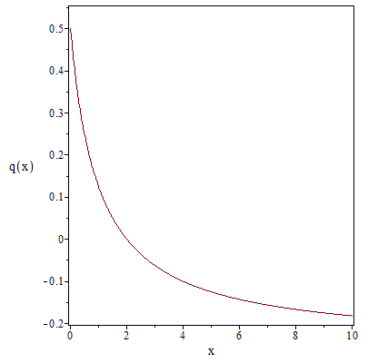
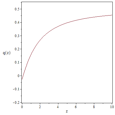
Figure 1: The evolution of the deceleration parameter is depicted for the particular minimal coupling model. The left diagram is with respect to the dimensionless parameter $x$, and the right diagram is with respect to the redshift with the parameter value $x(0)\simeq 7/3$ as a rough estimation.

4 Geodesic Deviation Equation

As mentioned, in the Einstein theory of gravitation, the physical significance of the Riemann tensor is demonstrated by the geodesic deviation concept. In this section, to investigate the relation between the nearby geodesics and how the flux of geodesics expands, we derive the GDE and the corresponding Raychaudhuri dynamical equation in the context of $f(R,T)$ modified gravity. Then, we mainly compare the results obtained for the particular minimal coupling model with the results of the previous section in order to have a better view on the cosmic acceleration phase. For this purpose, let us consider the general expression for the GDE [74, 75]

$$\frac{{{D^{2}}{\eta^{\mu}}}}{{D{\nu^{2}}}}+R^{\mu}{}_{\nu\alpha\beta}{V^{\nu}}{V^{\alpha}}{\eta^{\beta}}=0,$$ (39)

where the parametric equation is given by ${x^{\mu}}\left({\nu,s}\right)$, wherein $\nu$ is an affine parameter along the geodesics and $s$ labels distinct geodesics. Also, ${\eta^{\mu}}=d{x^{\mu}}/ds$ is the orthogonal deviation vector of two adjacent geodesics, the normalized vector field ${V^{\mu}}=d{x^{\mu}}/d\nu$ is tangent to the geodesics and ${D}/{D\nu}$ is the covariant derivative along the curve.

Now, to obtain the relation between the geometrical properties of the spacetime with the field equations governed from the modified gravitational theory, one can employ the well–known relation

$${R_{\mu\nu\alpha\beta}}={C_{\mu\nu\alpha\beta}}+\frac{1}{2}\left({{g_{\mu\alpha}}{R_{\nu\beta}}-{g_{\mu\beta}}{R_{\nu\alpha}}+{g_{\nu\beta}}{R_{\mu\alpha}}-{g_{\nu\alpha}}{R_{\mu\beta}}}\right)-\frac{1}{6}{R}\left({{g_{\mu\alpha}}{g_{\nu\beta}}-{g_{\mu\beta}}{g_{\nu\alpha}}}\right),$$ (40)

in $4$–dimensions. However, for the conformally flat spacetime, the Weyl tensor ${C_{\mu\nu\alpha\beta}}$ is identically zero. Then, by assumption ${f_{R}}\neq 0$, and inserting the Ricci tensor from the field equations (3) and the Ricci scalar from Eq. (5) into relation (40), we obtain

$$\begin{array}[]{l}{R_{\mu\nu\alpha\beta}}=\frac{1}{{2{f_{R}}}}\bigg{[}\left({\kappa+{f_{T}}}\right)\left({g_{\mu\alpha}}T_{\nu\beta}^{[m]}-{g_{\mu\beta}}T_{\nu\alpha}^{[m]}+{g_{\nu\beta}}T_{\mu\alpha}^{[m]}-{g_{\nu\alpha}}T_{\mu\beta}^{[m]}\right)+f\left({g_{\mu\alpha}}{g_{\nu\beta}}-{g_{\mu\beta}}{g_{\nu\alpha}}\right)\bigg{]}\\ \qquad\qquad+\frac{1}{{2{f_{R}}}}\left({g_{\mu\alpha}}{D_{\nu\beta}}-{g_{\mu\beta}}{D_{\nu\alpha}}+{g_{\nu\beta}}{D_{\mu\alpha}}-{g_{\nu\alpha}}{D_{\mu\beta}}\right){f_{R}}\\ \qquad\qquad-\frac{1}{{6{f_{R}}}}\bigg{[}{\left({\kappa+{f_{T}}}\right)T+2f-3\,{\Box}{f_{R}}}\bigg{]}\left({{g_{\mu\alpha}}{g_{\nu\beta}}-{g_{\mu\beta}}{g_{\nu\alpha}}}\right),\end{array}$$ (41)

where ${D_{\mu\nu}}\equiv{\nabla_{\mu}}{\nabla_{\nu}}-{g_{\mu\nu}{\Box}}$. Also, as assumed, for the dustlike matter flow as a perfect fluid, the energy–momentum tensor obviously is $T_{\mu\nu}^{[m]}={\rho^{[m]}}\,{u_{\mu}}u_{\nu}$, where ${u^{\mu}}$ is the comoving velocity vector to the matter flow with ${u_{\mu}}{u^{\mu}}=-1$, and hence, we get

$$\begin{array}[]{l}-R^{\mu}{}_{\nu\alpha\beta}{V^{\nu}}{V^{\alpha}}{\eta^{\beta}}=\\ \qquad\frac{1}{{2{f_{R}}}}\left[\left({\kappa+{f_{T}}}\right){{\rho^{[m]}}\left({\delta_{\alpha}^{\mu}{u_{\nu}}{u_{\beta}}-\delta_{\beta}^{\mu}{u_{\nu}}{u_{\alpha}}+{g_{\nu\beta}}{u^{\mu}}{u_{\alpha}}-{g_{\nu\alpha}}{u^{\mu}}{u_{\beta}}}\right)+f\left({\delta_{\alpha}^{\mu}{g_{\nu\beta}}-\delta_{\beta}^{\mu}{g_{\nu\alpha}}}\right)}\right]{V^{\nu}}{V^{\alpha}}{\eta^{\beta}}\\ \qquad+\frac{1}{{2{f_{R}}}}\left[{\left({\delta_{\alpha}^{\mu}{D_{\nu\beta}}-\delta_{\beta}^{\mu}{D_{\nu\alpha}}+{g_{\nu\beta}}D^{\mu}{}_{\alpha}-{g_{\nu\alpha}}D^{\mu}{}_{\beta}}\right){f_{R}}}\right]{V^{\nu}}{V^{\alpha}}{\eta^{\beta}}\\ \qquad-\frac{1}{{6{f_{R}}}}\left[{-\left({\kappa+{f_{T}}}\right){\rho^{[m]}}+2f-3\,{\Box}{f_{R}}}\right]\left({\delta_{\alpha}^{\mu}{g_{\nu\beta}}-\delta_{\beta}^{\mu}{g_{\nu\alpha}}}\right){V^{\nu}}{V^{\alpha}}{\eta^{\beta}}.\end{array}$$ (42)

By substituting the total energy $E=-{V_{\mu}}{u^{\mu}}$, $\varepsilon\equiv{V^{\mu}}{V_{\mu}}$, the relations ${\eta_{\mu}}{u^{\mu}}=0={\eta_{\mu}}{V^{\mu}}$ (note that, in the comoving frame, we have ${\eta^{0}}=0$), ${D_{00}}{f_{R}}=-3H{\dot{f}_{R}}$ and ${D_{ij}}{f_{R}}={g_{ij}}\left({{{\ddot{f}}_{R}}+2H{{\dot{f}}_{R}}}\right)$ into Eq. (42), the “force term” for the geodesic congruences yields

$$R^{\mu}{}_{\nu\alpha\beta}{V^{\nu}}{V^{\alpha}}{\eta^{\beta}}=\frac{-1}{{2{f_{R}}}}\left\{{\left[\left({\kappa+{f_{T}}}\right){{\rho^{[m]}}+{{\ddot{f}}_{R}}-H{{\dot{f}}_{R}}}\right]{E^{2}}+\frac{1}{3}\left[{{\rho^{[m]}}\left({\kappa+{f_{T}}}\right)+f+3{{\ddot{f}}_{R}}+3H{{\dot{f}}_{R}}}\right]{\varepsilon}}\right\}{\eta^{\mu}}.$$ (43)

As it is obvious, even if $f_{R}$ being a constant, due to $f_{T}\neq 0$, still some new terms appear into the corresponding GDE of the related model. Finally, by replacing Eqs. (14) and (15) into Eq. (43), we obtain

$$R^{\mu}{}_{\nu\alpha\beta}{V^{\nu}}{V^{\alpha}}{\eta^{\beta}}=-\frac{1}{2}\kappa^{[\rm eff]}\left[{\left({{\rho^{[\rm eff]}}+{p^{[\rm eff]}}}\right){E^{2}}+\frac{1}{3}\left({{\rho^{[\rm eff]}}+3{p^{[\rm eff]}}+\frac{R}{\kappa^{[\rm eff]}}}\right)\varepsilon}\right]{\eta^{\mu}}$$ (44)

for the FLRW metrics, which is a generalization of the Pirani equation [58]. Therefore, the GDE for the modified gravitational theory is

$$\frac{D^{2}\eta^{\mu}}{D\nu^{2}}+\frac{1}{2}\kappa^{[\rm eff]}\left[{\left({{\rho^{[\rm eff]}}+{p^{[\rm eff]}}}\right){E^{2}}+\frac{1}{3}\left({{\rho^{[\rm eff]}}+3{p^{[\rm eff]}}+\frac{R}{\kappa^{[\rm eff]}}}\right)\varepsilon}\right]{\eta^{\mu}}=0.$$ (45)

From the recent equation, one can obviously attain the GDE for the particular minimal coupling model and the $\Lambda$CDM model by inserting the corresponding Ricci scalar of each one of these models. In this regard, for the particular minimal coupling model, by substituting Eqs. (24), (25) and (26) into the GDE (45), gives

$$\frac{{{D^{2}}{\eta^{\mu}}}}{{D{\nu^{2}}}}+\frac{1}{2}\left[{\left({\kappa{\rho^{[m]}}+\frac{{\alpha\sqrt{{\rho^{[m]}}}}}{2}}\right){E^{2}}+\frac{2}{3}\left({\kappa{\rho^{[m]}}+\alpha\sqrt{{\rho^{[m]}}}}\right)\varepsilon}\right]{\eta^{\mu}}=0.$$ (46)

On the other hand, for the $\Lambda$CDM model, i.e. $f(R)=R-2\Lambda$, from the corresponding Eq. (5), we have

$$R=\kappa{\rho^{[m]}}+4\Lambda,$$ (47)

and Eqs. (14) and (15) result

$${\rho^{[{\mathop{\Lambda}}]}}=\frac{\Lambda}{\kappa}={-p^{[{\mathop{\Lambda}}]}}.$$ (48)

Thus, the GDE (45) for this case reads

$$\frac{D^{2}\eta^{\mu}}{D\nu^{2}}+\frac{1}{2}\left[\left(\kappa\rho^{[m]}\right){E^{2}}+\frac{2}{3}\left(\kappa\rho^{[m]}+\Lambda\right)\varepsilon\right]{\eta^{\mu}}=0.$$ (49)

The comparison of Eqs. (46) and (49) explicitly indicates the effect of $f_{T}\neq 0$.

In the following, we evaluate the timelike and the null geodesics in two subsections. However before we proceed, let us remind that, as we expect, each of the “force term” in these obtained GDEs is proportional to ${\eta^{\mu}}$ itself, and hence, only induces isotropic deviation. That is, in the FLRW case, we only have such a term which gives the spatial isotropy of spacetime, and the deviation vector ${\eta^{\mu}}$ only changes in magnitude but not in direction [57, 59]. Although, in an anisotropic universe, like the Bianchi I, the corresponding GDE also reflects a change in the direction of the deviation vector as shown in Ref. [76].

4.1 GDE For Timelike Vector Fields

For the timelike vector fields defined by the velocities of the comoving observers, within the spatially flat FLRW background, one has $\varepsilon=-1$, $E=1$ and the affine parameter $\nu$ matching with the proper time $t$ of the comoving fundamental observers up to a constant. Thus, the GDE (45) reduces to

$$\frac{{{D^{2}}{\eta^{\mu}}}}{{D{t^{2}}}}+\frac{1}{6{f_{R}}}\left({2\kappa{\rho^{\left[{\rm eff}\right]}}-R}\right){\eta^{\mu}}=0,$$ (50)

and hence, for the particular minimal coupling model, it reads

$$\frac{{{D^{2}}{\eta^{\mu}}}}{{D{t^{2}}}}+\frac{1}{6}\left({\kappa{\rho^{[m]}}-\frac{{\alpha\sqrt{{\rho^{[m]}}}}}{2}}\right){\eta^{\mu}}=0.$$ (51)

However, the deviation vector can be written in terms of the comoving tetrad frame (the Fermi–transported along unit tangent to geodesic) as ${\eta^{\mu}}=a\left(t\right){e^{\mu}}$, such that, it connects adjacent geodesics in the radial direction. Then, as isotropy (with no shear and spatial rotation) implies

$$\frac{{D{e^{\mu}}}}{{Dt}}=0,$$ (52)

therefore, Eq. (51) yields

$$\frac{{\ddot{a}}}{a}=-\frac{\kappa}{6}\left({{\rho^{\left[m\right]}}-\frac{{{\rho^{\left[{{\mathop{\rm int}}}\right]}}}}{2}}\right).$$ (53)

This equation is a particular case of the so called Raychaudhuri dynamical equation. Obviously, Eq. (53) indicates that if the dustlike matter dominates, the universe will decelerate and, when ${\rho^{{\mathop{[\rm int]}}}}=2{\rho^{[m]}}$, the acceleration for timelike geodesics vanishes. Also, in the late time universe (when ${\rho^{[\rm int]}}\gg{\rho^{[m]}}$), the acceleration occurs. These results are consistent with the results obtained in Sect. 3.

On the other hand, the GDE, for the timelike vector fields of the comoving observers in the $\Lambda$CDM model, gives

$$\frac{{\ddot{a}}}{a}=-\frac{1}{6}\left({\kappa{\rho^{[m]}}-2\Lambda}\right),$$ (54)

and when ${\rho^{[m]}}=2{\rho^{\left[\Lambda\right]}}$, the universe transition from the deceleration to the acceleration phase occurs. Also when ${\rho^{[\Lambda]}}\gg{\rho^{[m]}}$, we have an accelerated universe in the late time.

4.2 GDE For Null Vector Fields

In this subsection, we investigate the past–directed null vector fields, where in this case, still using the spatially flat FLRW background, one has $\varepsilon=0$. By considering ${\eta^{\mu}}=\eta{e^{\mu}}$ and using a parallelly propagated and aligned coordinate basis, i.e. ${D{e^{\mu}}/D\nu}={V^{\alpha}}{\nabla_{\alpha}}{e^{\mu}}=0$, the GDE (45) reduces to

$$\frac{{{d^{2}}\eta}}{{d{\nu^{2}}}}+\frac{1}{2}\kappa^{[\rm eff]}\left({{\rho^{[\rm eff]}}+{p^{[\rm eff]}}}\right){E^{2}}\eta=0.$$ (55)

At first, according to the general relativity (within the spatially flat FLRW spacetimes) discussed in Ref. [59], all families of the past–directed null geodesics experience focusing if provided the condition $\kappa\left({\rho+p}\right)>0$. In particular, for the cosmological constant case, in which the corresponding equation of state is ${p}=-{\rho}$, there is no focusing effect of the null geodesics. And hence, the solution of equation (55), in this particular case, is $\eta\left(\nu\right)={C_{1}}\nu+{C_{2}}$ (where ${C_{1}}$ and ${C_{2}}$ are integration constants) that is equivalent to the Minkowski spacetime. However, in this regard, the corresponding focusing condition for the $f(R,T)$ gravity model is

$${\kappa^{[\rm eff]}}\left({{\rho^{[\rm eff]}}+{p^{\left[{\rm eff}\right]}}}\right)>0.$$ (56)

Now, for the particular minimal coupling model, as the GDE (55) reads

$$\frac{{{d^{2}}{\eta}}}{{d{\nu^{2}}}}+\frac{1}{2}\left({\kappa{\rho^{[m]}}+\frac{{\alpha\sqrt{{\rho^{[m]}}}}}{2}}\right){E^{2}}{\eta}=0,$$ (57)

its focusing condition is actually provided when

$$\left({2{\rho^{[m]}}+{\rho^{\left[{{\mathop{\rm int}}}\right]}}}\right)>0$$ (58)

and, in turn, when $\sqrt{{\rho^{[m]}}}>-\alpha/(2\kappa)$ are satisfied, that is always confirmed for positive values of $\alpha$.

In continuation, it is more appropriate to write the deviation vector for the null geodesics as a function of the redshift rather than the proper time. This can obviously be performed through the transformation between the affine parameter and the redshift, where we also rewrite the GDE with respect to it. For this purpose, let us start by the simple differential operator

$$\frac{d}{{d\nu}}=\frac{{dz}}{{d\nu}}\frac{d}{{dz}},$$ (59)

that obviously yields

$$\frac{d^{2}}{d\nu^{2}}=\left(\frac{dz}{d\nu}\right)^{2}\frac{d^{2}}{dz^{2}}+\frac{d^{2}z}{d\nu^{2}}\frac{d}{dz}=\left(\frac{d\nu}{dz}\right)^{-2}\left[\frac{d^{2}}{dz^{2}}-(\frac{d\nu}{dz})^{-1}\frac{d^{2}\nu}{dz^{2}}\frac{d}{dz}\right].$$ (60)

Also, for the null geodesics, we have the well–known relation $(1+z)=a_{0}/a=E/E_{0}$, that by assuming ${a_{0}}=1$ (as the present–day value of the scale factor for the flat spacetime) and ${E_{0}}$ as a constant, leads to

$$\frac{{dz}}{{1+z}}=-\frac{{da}}{a}=\frac{{dE}}{E},$$ (61)

and thus, one obtains

$$dz=-\left({1+z}\right)\frac{{\dot{a}}}{a}\frac{{dt}}{{d\nu}}d\nu=-\left({1+z}\right)HEd\nu.$$ (62)

However, by substituting for $E$, one can rewrite Eq. (62) as

$$\frac{{d\nu}}{{dz}}=-\frac{1}{{{E_{0}}H{{\left({1+z}\right)}^{2}}}},$$ (63)

and hence, gets

$$\frac{{{d^{2}}\nu}}{{d{z^{2}}}}=\frac{1}{{{E_{0}}H{{\left({1+z}\right)}^{3}}}}\left[{2+\frac{{\left({1+z}\right)}}{H}\left({\frac{{dH}}{{dz}}}\right)}\right].$$ (64)

Besides, we have

$$\frac{{dH}}{{dz}}=\frac{{d\nu}}{{dz}}\frac{{dt}}{{d\nu}}\frac{{dH}}{{dt}}=-\frac{{\dot{H}}}{{H\left({1+z}\right)}},$$ (65)

that by replacing it into Eq. (64), leads to

$$\frac{{{d^{2}}\nu}}{{d{z^{2}}}}=\frac{1}{{{E_{0}}H{{\left({1+z}\right)}^{3}}}}\left({2-\frac{{\dot{H}}}{{{H^{2}}}}}\right).$$ (66)

On the other hand, from the definition of the Hubble parameter, one obviously has $\dot{H}={\ddot{a}}/a-{H^{2}}$, that by inserting it into Eq. (66), while using Eq. (17), gives

$$\frac{{{d^{2}}\nu}}{{d{z^{2}}}}=\frac{1}{{{E_{0}}H{{\left({1+z}\right)}^{3}}}}\left[{3+\frac{{{\kappa^{\left[{\rm eff}\right]}}\left({{\rho^{\left[{\rm eff}\right]}}+3{p^{\left[{\rm eff}\right]}}}\right)}}{{6{H^{2}}}}}\right].$$ (67)

Finally, by substituting Eqs. (63) and (67) into Eq. (60), we obtain

$$\frac{{{d^{2}}\eta}}{{d{\nu^{2}}}}=E_{0}^{2}{H^{2}}{\left({1+z}\right)^{4}}\left\{{\frac{{{d^{2}}\eta}}{{d{z^{2}}}}+\frac{1}{{\left({1+z}\right)}}\left[{3+\frac{{{\kappa^{\left[{\rm eff}\right]}}\left({{\rho^{\left[{\rm eff}\right]}}+3{p^{\left[{\rm eff}\right]}}}\right)}}{{6{H^{2}}}}}\right]\frac{{d\eta}}{{dz}}}\right\},$$ (68)

where, by inserting Eq. (55) into it, leads to the null GDE corresponding to the modified gravity as

$$\frac{{{d^{2}}\eta}}{{d{z^{2}}}}+\frac{3}{{1+z}}\left[{1+\frac{{{\kappa^{[\rm eff]}}}}{{18{H^{2}}}}\left({{\rho^{[\rm eff]}}+3{p^{[\rm eff]}}}\right)}\right]\frac{{d\eta}}{{dz}}+\frac{{{\kappa^{[\rm eff]}}}}{{2{{\left({1+z}\right)}^{2}}{H^{2}}}}\left({{\rho^{[\rm eff]}}+{p^{[\rm eff]}}}\right)\eta=0.$$ (69)

Also, by substituting ${\rho^{[\rm eff]}}$ and ${p^{[\rm eff]}}$ from definitions (16) and (20) into Eq. (69), reduces the null GDE as

$$\frac{{{d^{2}}\eta}}{{d{z^{2}}}}+\frac{{\left({7+3{w^{[\rm eff]}}}\right)}}{{2\left({1+z}\right)}}\frac{{d\eta}}{{dz}}+\frac{{3\left({1+{w^{[\rm eff]}}}\right)}}{{2{{\left({1+z}\right)}^{2}}}}\eta=0,$$ (70)

where it obviously depends only on ${w^{[\rm eff]}}$ as a function of the redshift, i.e. as a function of the cosmological evolution.

At last, by inserting Eq. (30) into (70), we can obtain the GDE for the particular minimal coupling model as

$$\frac{d^{2}\eta}{dz^{2}}+\frac{14+11x(z)}{4\left(1+z\right)\left(1+x(z)\right)}\frac{d\eta}{dz}+\frac{3\left(2+x(z)\right)}{4\left(1+z\right)^{2}\left(1+x(z)\right)}\eta=0,$$ (71)

where again $x(z)=x(0)/(1+z)^{3/2}$ up to the present. This equation has a $Q$–Legendre solution as

$$\eta\left(z\right)=\frac{{{C_{1}}}}{{1+z}}+\frac{{{C_{2}}}}{{{{\left({1+z}\right)}^{7/8}}}}Q_{-1/6}^{1/6}\left({\frac{{\sqrt{49+\left({21z+21}\right)\sqrt{1+z}}}}{7}}\right),$$ (72)

where $C_{1}$ and $C_{2}$ are integration constants related to $x(0)$. As appropriate initial conditions, we set, at $z=0$, the deviation vector to be zero and its first derivative to be $1$, and then, plot the deviation vector with respect to the redshift in the left diagram of Fig. $2$, wherein the corresponding term of the $\Lambda$CDM model has also been numerically drawn for comparison.

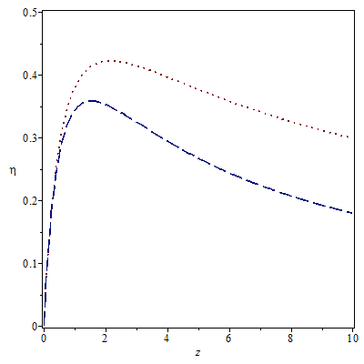
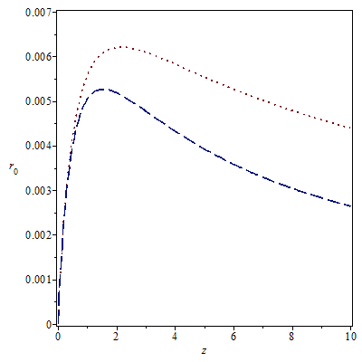
Figure 2: The deviation vector (left) and the observer area–distance (right) are depicted with respect to the redshift, for the $\Lambda$CDM model (the dotted curve) and for the particular minimal coupling model (the dashed curve), with the appropriate initial conditions $\eta(z)|_{z=0}=0$ and $d\eta(z)/dz|_{z=0}=1$, and the parametric values $H_{0}\simeq 68$ (km/s)/Mpc and $x(0)\simeq 7/3$ as rough estimations.

Now, we are in a position to indicate the observer area–distance, ${r_{0}}$, first derived by Mattig [64]. At first, in a spherically symmetric spacetime, for instance in the FLRW universes, the magnitude of the deviation vector $\eta$ is related with the proper area $dA$ of a source in a redshift $z$ as $d\eta\propto\sqrt{dA}$, and hence, the observer area–distance can be found as a function of the redshift in units of the present–day Hubble radius $H_{0}^{-1}$, see, e.g., Ref. [80]. That is, by its definition, we get

$${r_{0}}\left(z\right):=\sqrt{\left|{\frac{{d{A_{0}}\left(z\right)}}{{d\Omega}_{0}}}\right|}=\left|{\frac{{\eta\left({z^{\prime}}\right)\left|{{}_{z^{\prime}=z}}\right.}}{{d\eta\left({z^{\prime}}\right)/dl\left|{{}_{z^{\prime}=0}}\right.}}}\right|,$$ (73)

where ${A_{0}}$ is the area of the object, $\Omega$ is the solid angle and $dl=a\left(t\right)dr$ with r as the comoving radial coordinate in the FLRW metrics. Using the fact that $d/dl=H\left({1+z}\right)d/dz$ and choosing the deviation vector to be zero at $z=0$, thus ${r_{0}}$ reads

$${r_{0}}\left(z\right)=\left|{\frac{{\eta\left(z\right)}}{H(0){d\eta\left({z^{\prime}}\right)/dz^{\prime}\left|{{}_{z^{\prime}=0}}\right.}}}\right|,$$ (74)

where practically $H(0)$ can be evaluated from the modified Friedmann equation (28) at $z=0$. Analytical expression for the observer area–distance in general relativity with no cosmological constant obtained in Refs. [59, 81]. However, in our case, the plot of Eq. (74) for the particular minimal coupling model has been depicted in the right diagram of Fig. $2$ while employing the solution of the deviation vector in the left diagram of it with the approximate value of $68$ (km/s)/Mpc for $H_{0}$ [8].

The comparison of the diagrams of Fig. $2$ with the corresponding diagrams of the $\Lambda$CDM model in Refs. [59, 70] illustrates that the general behavior of the null geodesic deviation and the observer area–distance in the particular minimal coupling model are almost similar to the $\Lambda$CDM model. Hence, this model can remain phenomenologically viable and being tested with the observational data. Also, the comparison of the results of the model, with the corresponding results of the Hu–Sawicki models (considered in Ref. [70]) and the $f(T)$ gravity (obtained in Ref. [71]), shows, in general, similar behaviors for the null geodesic deviation and the observer area–distance.

5 Conclusions

We have considered the $f(R,T)$ modified gravity, in particular, have focused on the minimal coupling of the matter and geometry within the homogeneous and isotropic spatially flat FLRW background. Considering this particular case of the theory, by the requirement of the conservation law of the energy–momentum tensor, we choose the model to be a simple and the most plausible of the form $f(R,T)=R-\alpha\sqrt{-T}$, with $\alpha$ as a positive and adjustable constant. Also, we assume that the universe is made of the dustlike matter and a perfect fluid for the interaction/coupling between the matter and geometry. Then, by the fact that the density of the matter reduces by the time, we compare it with the constant value of $\left(\alpha/\kappa\right)^{2}$ as a criterion. Hence, we have shown that, the case ${\rho^{[m]}}\gg\left(\alpha/\kappa\right)^{2}$ corresponds to the matter dominated epoch with a decelerated evolution, and the case ${\rho^{[m]}}\ll\left(\alpha/\kappa\right)^{2}$ is related to an accelerated phase. To study the cosmology of the model in the matter dominated and the acceleration phases, we have obtained some cosmological parameters such as the state and the deceleration parameters. We find that the value of the state parameter in the coupling density dominated is less than $-1/3$ and the deceleration parameter attains a negative value, thus, an accelerated universe arises by the coupling between the matter and geometry. It has been indicated that, when $\rho^{[m]}={({\alpha/2\kappa})^{2}}$, the deceleration parameter is zero, and the universe has a transition from the deceleration phase to the acceleration one. Also, we have shown that the coupling energy density depends on the Hubble parameter, and thus, with the passage of the time, it gets larger than the matter density. Although we find that the minimal coupling model causes an acceleration phase, but its obtained equation of state parameter is less than the corresponding observed data. Nevertheless, if one considers a more general model, yet in this context but with non–conserved interaction energy–momentum tensor, then, one would expect to get results more closer to the observations.

On the other hand, to make our investigations more instructive, we have also scrutinized the motion of the free test particles on their geodesics, and have obtained the GDE in context of the $f(R,T)$ modified gravity, which provides an elegant tool to investigate the structure of the spacetime, and to describe the relative acceleration of the neighboring geodesics as a measurable physical quantity. The coupling between the matter and curvature leads to the appearance of the new internal “force terms” in the GDE. Moreover, through the corresponding GDE, we have derived the generalized Pirani equation for the chosen model. Then, we have investigated the timelike and the null vector fields in this type of modified theory. The case of fundamental observers gives us the generalized Raychaudhuri equation. Also, we have obtained the observer area–distance for this case, and have plotted the results with respect to the redshift. We have shown that the null deviation vector fields and the observer area–distance, in the model, have an evolution almost similar to the corresponding ones in the $\Lambda$CDM model, the Hu–Sawicki models of $f(R)$ theory and the $f(T)$ gravity.

Appendix

From the definition of the interaction/coupling energy–momentum tensor, Eq. (7), one has

$$\kappa{\nabla^{\mu}}T_{\mu\nu}^{[{\mathop{\rm int}}]}={\nabla^{\mu}}\left[{{f_{T}}T_{\mu\nu}^{[m]}+\frac{1}{2}\left({f-R{f_{R}}}\right){g_{\mu\nu}}+\left({{\nabla_{\mu}}{\nabla_{\nu}}-{g_{\mu\nu}}}\Box\right){f_{R}}}\right],$$ (75)

wherein using the definition of Einstein tensor, it reads

$$\kappa{\nabla^{\mu}}T_{\mu\nu}^{[{\mathop{\rm int}}]}={\nabla^{\mu}}\left[{{f_{T}}T_{\mu\nu}^{[m]}+\frac{f}{2}{g_{\mu\nu}}+{f_{R}}{G_{\mu\nu}}-{f_{R}}{R_{\mu\nu}}+\left({{\nabla_{\mu}}{\nabla_{\nu}}-{g_{\mu\nu}}}\Box\right){f_{R}}}\right].$$ (76)

As for any scalar and vector fields, one has ${\nabla_{\mu}}{\nabla_{\nu}}\varphi={\nabla_{\nu}}{\nabla_{\mu}}\varphi$  and

$${\nabla_{\mu}}{\nabla_{\nu}}{A_{\alpha}}-{\nabla_{\nu}}{\nabla_{\mu}}{A_{\alpha}}={R_{\alpha\beta\mu\nu}}{A^{\beta}},$$ (77)

thus, one gets

$${\nabla^{\mu}}{\nabla_{\mu}}{\nabla_{\nu}}{f_{R}}={\nabla^{\mu}}{\nabla_{\nu}}{\nabla_{\mu}}{f_{R}}={\nabla_{\nu}}{\nabla^{\mu}}{\nabla_{\mu}}{f_{R}}+{R_{\mu\alpha}}{{}^{\mu}_{\nu}}{\nabla^{\alpha}}{f_{R}}={\nabla_{\nu}}\square{f_{R}}+{R_{\mu\nu}}{\nabla^{\mu}}{f_{R}}.$$ (78)

Also, by

$${\nabla_{\nu}}f\left({R,T}\right)={f_{R}}{\nabla_{\nu}}R+{f_{T}}{\nabla_{\nu}}T$$ (79)

and

$${\nabla^{\mu}}{G_{\mu\nu}}=0\qquad\Rightarrow\qquad{\nabla^{\mu}}{R_{\mu\nu}}=\frac{1}{2}{\nabla_{\nu}}R,$$ (80)

one attains

$$\frac{{{g_{\mu\nu}}}}{2}\left({{\nabla^{\mu}}f}\right)-{f_{R}}\left({{\nabla^{\mu}}{R_{\mu\nu}}}\right)=\frac{1}{2}{f_{T}}{\nabla_{\nu}}T.$$ (81)

Knowing ${\nabla_{\mu}}{g_{\alpha\beta}}=0$, and substituting relations (78) and (81) into relation (76), leads to

$$\kappa{\nabla^{\mu}}T_{\mu\nu}^{[{\mathop{\rm int}}]}=T_{\mu\nu}^{[m]}{\nabla^{\mu}}{f_{T}}+{G_{\mu\nu}}{\nabla^{\mu}}{f_{R}}+\frac{1}{2}{f_{T}}{\nabla_{\nu}}T$$ (82)

wherein, with relation (8), it poses some restrictions on the choice of the function of $f(R,T)$ on $T$ as

$$T_{\mu\nu}^{[m]}{\nabla^{\mu}}{f_{T}}+\frac{1}{2}{f_{T}}{\nabla_{\nu}}T=0.$$ (83)

Note that, such restrictions not only do not contradict with the diffeomorphism invariance of the action (1), but they also arise out of it. That is, the price for a priori inclusion of the trace of the energy–momentum tensor (that itself will emerge from the variation of the Lagrangian of the matter, definition (2)) is to have these restrictions as self–consistency.

Now, writing the result for the index $\nu=0$ of the comoving FLRW metrics, it yields

$$-T_{00}^{[m]}{\dot{f}_{T}}+\frac{1}{2}{f_{T}}{\dot{T}^{[m]}}=0,$$ (84)

and by substituting $T_{00}^{[m]}={\rho^{[m]}}$ and ${\dot{T}}=-{\dot{\rho}^{[m]}}=3H{\rho^{[m]}}$, one achieves the constraint equation (10).

References

- [1] A.G. Riess, et al., “Observational evidence from supernovae for an accelerating universe and a cosmological constant”, Astron. J. 116, 1009 (1998).
- [2] S. Perlmutter, et al. [The Supernova Cosmology Project], “Measurements of Omega and Lambda from high–redshift supernovae”, Astrophys. J. 517, 565 (1999).
- [3] A.G. Riess, et al., “BV RI light curves for type Ia supernovae”, Astron. J. 117, 707 (1999).
- [4] A.G. Riess, et al., “Type Ia supernova discoveries at from the Hubble space telescope: Evidence for past deceleration and constraints on dark energy evolution”, Astrophys. J. 607, 665 (2004).
- [5] J.P. Ostriker and P.J. Steinhardt, “Cosmic concordance”, arXiv: astro-ph/9505066.
- [6] S.M. Carroll, “The cosmological constant”, Living. Rev. Rel. 4, 1 (2001).
- [7] P.A.R. Ade, et al. [Planck Collaboration], “Planck 2013 results. XVI. Cosmological parameters”, Astron. Astrophys. 571, A16 (2014).
- [8] P.A.R. Ade, et al. [Planck Collaboration], “Planck 2015 results. XIII. Cosmological parameters”, arXiv: 1502.01589.
- [9] S. Weinberg, “The cosmological constant problem”, Rev. Mod. Phys. 61, 1 (1989).
- [10] V. Sahni, “The cosmological constant problem and quintessence”, Class. Quant. Grav. 19, 3435 (2002).
- [11] S. Nobbenhuis, “Categorizing different approaches to the cosmological constant problem”, Found. Phys. 36, 613 (2006).
- [12] H. Padmanabhan and T. Padmanabhan, “CosMIn: The solution to the cosmological constant problem”, Int. J. Mod. Phys. D 22, 1342001 (2013).
- [13] D. Bernard and A. LeClair, “Scrutinizing the cosmological constant problem and a possible resolution”, Phys. Rev. D 87, 063010 (2013).
- [14] P.J.E. Peebles and B. Ratra, “The cosmological constant and dark energy”, Rev. Mod. Phys. 75, 559 (2003).
- [15] T. Padmanabhan, “Cosmological constant–the weight of the vacuum”, Phys. Rep. 380, 235 (2003).
- [16] D. Polarski, “Dark energy: Current issues”, Ann. Phys. (Berlin) 15, 342 (2006).
- [17] E.J. Copeland, M. Sami and S. Tsujikawa, “Dynamics of dark energy”, Int. J. Mod. Phys. D 15, 1753 (2006).
- [18] R. Durrer and R. Maartens, “Dark energy and dark gravity: Theory overview”, Gen. Rel. Grav. 40, 301 (2008).
- [19] K. Bamba, S. Capozziello, S. Nojiri and S.D. Odintsov, “Dark energy cosmology: The equivalent description via different theoretical models and cosmography tests”, Astrophys. Space Sci. 342, 155 (2012).
- [20] A.F. Bahrehbakhsh, M. Farhoudi and H. Vakili, “Dark energy from fifth dimensional Brans–Dicke theory”, Int. J. Mod. Phys. D 22, 1350070 (2013).
- [21] R. Bean and O. Dore, “Are chaplygin gases serious contenders for the dark energy?”, Phys. Rev. D 68, 023515 (2003).
- [22] T. Multamaki, M. Manera and E. Gaztanaga, “Large scale structure and the generalized chaplygin gas as dark energy”, Phys. Rev. D 69, 023004 (2004).
- [23] H. Farajollahi, M. Farhoudi, A. Salehi and H. Shojaie, “Chameleonic generalized Brans–Dicke model and late–time acceleration”, Astrophys. Space Sci. 337, 415 (2012).
- [24] S. Capozziello, V.F. Cardone, S. Carloni and A. Troisi, “Curvature quintessence matched with observational data”, Int. J. Mod. Phys. D 12, 1969 (2003).
- [25] S. Nojiri and S.D. Odintsov, “Introduction to modified gravity and gravitational alternative for dark energy”, Int. J. Geom. Meth. Mod. Phys. 04, 115 (2007).
- [26] L. Amendola, R. Gannouji, D. Polarski and S. Tsujikawa, “Conditions for the cosmological viability of dark energy models”, Phys. Rev. D 75, 083504 (2007).
- [27] L. Amendola and S. Tsujikawa, Dark Energy: Theory and Observations, (Cambridge University Press, Cambridge, 2010).
- [28] A.F. Bahrehbakhsh, M. Farhoudi and H. Shojaie, “FRW cosmology from five dimensional vacuum Brans–Dicke theory”, Gen. Rel. Grav. 43, 847 (2011).
- [29] T. Chiba, “ gravity and scalar–tensor gravity”, Phys. Lett. B 575, 1 (2003).
- [30] S.M. Carroll, V. Duvvuri, M. Trodden and M.S. Turner, “Is cosmic speed–up due to new gravitational physics?”, Phys. Rev. D 70, 043528 (2004).
- [31] V. Faraoni, “Matter instability in modified gravity”, Phys. Rev. D 74, 104017 (2006).
- [32] K. Atazadeh, M. Farhoudi and H.R. Sepangi, “Accelerating universe in brane gravity”, Phys. Lett. B 660, 275 (2008).
- [33] E.E. Flanagan, “Higher order gravity theories and scalar tensor theories”, Class. Quant. Grav. 21, 417 (2004).
- [34] T.P. Sotiriou, “ gravity and scalar–tensor theory”, Class. Quant. Grav. 23, 5117, (2006).
- [35] M. Farhoudi, “On higher order gravities, their analogy to GR, and dimensional dependent version of Duff’s trace anomaly relation”, Gen. Rel. Grav. 38, 1261 (2006).
- [36] H.–J. Schmidt, “Fourth order gravity: Equations, history, and applications to cosmology”, Int. J. Geom. Methods Mod. Phys. 4, 209 (2007).
- [37] A. De Felice and S. Tsujikawa, “ theories”, Living Rev. Rel. 13, 3 (2010).
- [38] T.P. Sotiriou and V. Faraoni, “ theories of gravity”, Rev. Mod. Phys. 82, 451 (2010).
- [39] S. Capozziello and M. De Laurentis, “Extended theories of gravity”, Phys. Rep. 509, 167 (2011).
- [40] S. Capozziello and V. Faraoni, Beyond Einstein Gravity: A Survey of Gravitational Theories for Cosmology and Astrophysics, (Springer, London, 2011).
- [41] S. Nojiri and S.D. Odintsov, “Unified cosmic history in modified gravity: From theory to Lorentz non–invariant models”, Phys. Rep. 505, 59 (2011).
- [42] T. Clifton, P.G. Ferreira, A. Padilla and C. Skordis, “Modified gravity and cosmology”, Phys. Rep. 513, 1 (2012).
- [43] T. Harko, “Modified gravity with arbitrary coupling between matter and geometry”, Phys. Lett. B 669, 376 (2008).
- [44] T. Harko, F.S.N. Lobo, S. Nojiri and S.D. Odintsov, “ gravity”, Phys. Rev. D 84, 024020 (2011).
- [45] Y. Bisabr, “Modified gravity with a nonminimal gravitational coupling to matter”, Phys. Rev. D 86, 044025 (2012).
- [46] M. Jamil, D. Momeni, R. Muhammad and M. Ratbay, “Reconstruction of some cosmological models in gravity”, Eur. Phys. J. C 72, 1999 (2012).
- [47] F.G. Alvarenga, A. de la Cruz–Dombriz, M.J.S. Houndjo, M.E. Rodrigues and D. Sáez–Gómez, “Dynamics of scalar perturbations in gravity”, Phys. Rev. D 87, 103526 (2013).
- [48] Z. Haghani, T. Harko, F.S.N. Lobo, H.R. Sepangi and S. Shahidi, “Further matters in spacetime geometry: gravity”, Phys. Rev. D 88, 044023 (2013).
- [49] H. Shabani and M. Farhoudi, “ cosmological models in phase space”, Phys. Rev. D 88, 044048 (2013).
- [50] H. Shabani and M. Farhoudi, “Cosmological and solar system consequences of gravity models”, Phys. Rev. D 90, 044031 (2014).
- [51] Z. Haghani, T. Harko, H.R. Sepangi and S. Shahidi, “Matter may matter”, Int. J. Mod. Phys. D 23, 1442016 (2014).
- [52] H. Shabani, “Cosmological consequences and statefinder diagnosis of non–interacting generalized chaplygin gas in gravity”, arXiv:1604.04616.
- [53] H. Shabani and A.H. Ziaie, “Stability of the Einstein static universe in gravity”, arXiv:1606.07959.
- [54] N.D. Birrell and P.C.W. Davies, Quantum Fields in Curved Space, (Cambridge University Press, Cambridge, 1982).
- [55] M. Farhoudi, “Classical trace anomaly”, Int. J. Mod. Phys. D 14, 1233 (2005).
- [56] M. Farhoudi, Non–linear Lagrangian Theories of Gravitation, (Ph.D. thesis, Queen Mary and Westfield College, University of London, 1995).
- [57] J.L. Synge, “On the deviation of geodesics and null–geodesics, particularly in relation to the properties of spaces of constant curvature and indefinite line–element”, Ann. Math. 35, 705 (1934), Republished in: Gen. Rel. Grav. 41, 1205 (2009).
- [58] F.A.E. Pirani, “On the physical significance of the Riemann tensor”, Acta Phys. Polon. 15, 389 (1956), Republished in: Gen. Rel. Grav. 41, 1215 (2009).
- [59] G.F.R. Ellis and H. van Elst, “Deviation of geodesics in FLRW spacetime geometries”, arXiv: gr-qc/9709060.
- [60] P. Szekeres, “The gravitational compass”, J. Maths. Phys. 6, 1387 (1965).
- [61] C.W. Misner, K.S. Thorne and J.A. Wheeler, Gravitation, (Freeman and Company, New York, 1973).
- [62] F.A.E. Pirani, “Invariant formulation of gravitational radiation theory”, Phys. Rev. 105, 1089 (1957).
- [63] A. Raychaudhuri, “Relativistic cosmology I.”, Phys. Rev. 98, 1123 (1955).
- [64] W. Mattig, “Über den Zusammenhang zwischen Rotverschiebung und scheinbarer Helligkeit (About the relation between redshift and apparent magnitude)”, Astron. Nachr. 284, 109 (1957).
- [65] C. Clarkson, G.F.R. Ellis, A. Faltenbacher, R. Maartens, O. Umeh and J.–P. Uzan, “(Mis)interpreting supernovae observations in a lumpy universe”, Mon. Not. R. Astron. Soc. 426, 1121 (2012).
- [66] F. Shojai and A. Shojai, “Geodesic congruences in the Palatini theory”, Phys. Rev. D 78, 104011 (2008).
- [67] A. Guarnizo, L. Castaneda and J.M. Tejeiro, “Geodesic deviation equation in gravity”, Gen. Rel. Grav. 43, 2713 (2011).
- [68] A. Guarnizo, L. Castaneda and J.M. Tejeiro, “Erratum to: Geodesic Deviation Equation in gravity”, Gen. Rel. Grav. 47, 109 (2015).
- [69] T. Harko, F.S.N. Lobo, “Geodesic deviation, Raychaudhuri equation, and tidal forces in modified gravity with an arbitrary curvature–matter coupling”, Phys. Rev. D 86, 124034 (2012).
- [70] A. de la Cruz–Dombriz, P.K.S. Dunsby, V.C. Busti and S. Kandhai, “Tidal forces in theories of gravity”, Phys. Rev. D 89, 064029 (2014).
- [71] F. Darabi, M. Mousavi and K. Atazadeh, “Geodesic deviation equation in gravity”, Phys. Rev. D 91, 084023 (2015).
- [72] W. Hu and I. Sawicki, “Models of cosmic acceleration that evade solar–system tests”, Phys. Rev. D 76, 064004 (2007).
- [73] A. Friedmann, “On space curvature”, Z. Phys. 10, 377 (1922).
- [74] R.M. Wald, General Relativity, (University of Chicago, Chicago, 1984).
- [75] R. d’Inverno, Introducing Einstein’s Relativity, (Clarendon Press, Oxford, 1992).
- [76] D.L. Caceres, L. Castaneda and J.M. Tejeiro, “Geodesic deviation equation in Bianchi cosmologies”, J. Phys. Conf. Ser. 229, 012076 (2010).
- [77] F.D. Albareti, J.A.R. Cembranos and A. de la Cruz–Dombriz, “Focusing of geodesic congruences in an accelerated expanding universe”, J. Cosmol. Astropart. Phys. 12, 020 (2012).
- [78] J. Santos, J.S. Alcaniz, M.J. Rebouças and F.C. Carvalho, “Energy conditions in –gravity”, Phys. Rev. D 76, 083513 (2007).
- [79] F. D. Albareti, J.A.R. Cembranos, A. de la Cruz–Dombriz and A. Dobado, “On the non–attractive character of gravity in theories”, J. Cosmol. Astropart. Phys. 07, 009 (2013).
- [80] P. Schneider, J. Ehlers and E.E. Falco, Gravitational Lenses, (Springer–Verlag, Berlin, 1992).
- [81] D.R. Matravers and A.M. Aziz, “A note on the observer area–distance formula”, Mon. Not. R. Astron. Soc. 47, 124 (1988).