Testing the blazar sequence with the least luminous BL Lacs.

In a previous paper, we proposed a new method to select low-power BL Lacs (LPBLs) based on mid-infrared emission and flux contrast through the Ca II spectral break; that study led to the selection of a complete sample formed by 34 LPBLs with $0.05<z\leq 0.15$ and radio luminosities spanning the range $\log L_{\rm r}=39.2$–41.5 [$\rm erg\,s^{-1}$]. We now assemble the broadband spectral energy distributions (SEDs) of these sources to investigate their nature and compare them with brighter BL Lacs. We find that the ratios between the X-ray and radio luminosities range from $\sim 20$ to $\sim 30000$ and that the synchrotron peak frequencies span a wide energy interval, from $\log\rm\,\nu_{\rm peak}\sim 13.5$ to $\sim 20$ [Hz]. This indicates a broad variety of SED shapes and a mixture of BL Lac flavors. Indeed, although the majority of our LPBLs are high-energy peaked BL Lacs (HBLs), we find that a quarter of them are low-energy peaked BL Lacs (LBLs), despite the fact that the sample is biased against the selection of LBLs. The analysis of the median LPBL SED confirms disagreement with the blazar sequence at low radio luminosities. Furthermore, if we limit the sample to the LBLs subsample, we find that their median SED shape is essentially indistinguishable from that of the most luminous BL Lacs. We conclude that the observed radio power is not the main driving parameter of the multiwavelength properties of BL Lacs.

1 Introduction

Blazars are active galactic nuclei (AGNs) showing extreme properties. Their flux variability at all wavelengths, high and variable polarization, apparent superluminal motion of the radio knots, and high brightness temperatures are all signatures of relativistic motion in a plasma jet that is oriented at a small angle with respect to the line of sight. The consequent Doppler beaming of the nonthermal jet emission usually makes this emission dominate over the thermal emission from both the AGN nucleus (accretion disk, broad and narrow line regions, dusty torus) and the host galaxy. Therefore, the study of blazar emission is the most efficient tool to unveil the nature of extragalactic jets.

Blazars include flat-spectrum radio quasars (FSRQs) and BL Lac objects. The classical distinction between them is based on the strength of the emission lines, whose rest-frame equivalent width (EW) must be smaller than 5 Å to define a BL Lac (Stickel et al., 1991). Another quantity used to identify blazars is the value of the flux density contrast across the Ca II spectral break (Stocke et al., 1991), which is reduced with respect to that of quiescent galaxies in case of a nonthermal contribution.

BL Lacs were further divided into radio-selected BL Lacs (RBL) and X-ray selected BL Lacs (XBL) until Padovani & Giommi (1995) proposed a more physical classification into high-energy cutoff BL Lacs (HBL) and low-energy cutoff BL Lacs (LBL), setting the dividing line between the two classes at $F_{\rm x}/F_{\rm r}\sim 200$, where $F_{\rm x}$ is the 0.3–3.5 keV flux and $F_{\rm r}=\nu F_{\nu}$ at 5 GHz. In the usual $\log\nu\,F_{\nu}$ versus $\log\nu$ representation, the blazar spectral energy distribution (SED) shows two main bumps corresponding to the synchrotron (from radio to UV or X-rays) and inverse-Compton (from X to $\gamma$ rays) jet emission contributions. In the LBL SED, the synchrotron peak falls in the infrared–optical band, while it is in the UV–X-rays in HBL. The operation of new TeV Telescopes, such as the Major Atmospheric Gamma Imaging Cherenkov Telescopes (MAGIC), the High Energy Stereoscopic System (H.E.S.S.) and the Very Energetic Radiation Imaging Telescope Array System (VERITAS), and the planning of more sophisticated TeV instruments, such as the Cherenkov Telescope Array (CTA; Acharya et al., 2013) has called attention to the extremely high-energy peaked BL Lacs (EHBL). Following Bonnoli et al. (2015), they are characterized by $F_{\rm x}/F_{\rm r}\ga 10^{4}$, where $F_{\rm x}$ is the X-ray flux in the 0.1-2.4 keV band, and $F_{\rm r}=\nu F_{\nu}$ at 1.4 GHz.

Fossati et al. (1998; hereafter F98) proposed a unifying view of the blazar SED behavior. These authors suggested that when the radio power decreases the synchrotron peak frequency shifts to higher energies and the Compton dominance, i.e., the ratio between the inverse-Compton and synchrotron peak luminosities, decreases. In this way, FSRQs, LBLs, and HBLs form a continuous spectral sequence, which is the so-called “blazar sequence”. This picture was subsequently confirmed by Donato et al. (2001), who also included hard X-ray data in the analysis. However, some authors have criticized this view. On one side, the existence of high-power HBL has been claimed (see, e.g., Padovani et al., 2003; Giommi et al., 2012). On the other side, LBL of low power have been found in deeper radio-selected samples (Padovani et al., 2003; Caccianiga & Marchã, 2004; Antón & Browne, 2005). These authors argued that the blazar sequence of F98 may be the result of selection biases because the high-power sources were mostly radio-selected objects, while the low-power sources were mainly X-ray selected objects (see also Landt & Bignall, 2008). Moreover, Nieppola et al. (2008) suggested that the anticorrelation between synchrotron peak frequency and luminosity disappears when correcting for the relativistic Doppler boosting effect. The blazar sequence has then been revisited by Ghisellini & Tavecchio (2008), who substituted the dependence of the jet emission properties on the jet power alone with a dependence on two parameters, namely the black hole mass and accretion rate. The accretion rate has also been invoked by Meyer et al. (2011) as a second parameter needed to define the SED features.

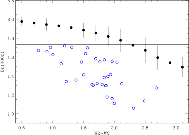
Figure 1: The LPBLs identified in Paper I (blue circles). They lie in the “forbidden zone” of the Dn(4000) versus the W2-W3 diagram, which is defined by the Dn(4000) limit obtained by requiring that the nonthermal jet contribution is at least 1/3 of the host galaxy one at 3900 Å, and by the 1-sigma lower limit to the average relation holding for the 21065 bright nearby galaxies (black dots; see Paper I for details).

The least luminous blazars are extremely interesting because they enable us to explore the behavior of the blazars properties at very low radio power and they probe the jet formation and emission processes at the lowest levels of accretion. These sources allow us to test the low-power end of the blazar sequence, which predicts that they are all HBLs. A major difficulty in finding low-luminosity BL Lacs comes from the dilution of the jet emission by the host starlight in the optical and near-IR bands. In Capetti & Raiteri (2015, hereafter Paper I), we proposed a new method to select low-power BL Lacs (LPBLs) based on a new diagnostic plane that includes the W2$-$W3 color from the Wide-Field Infrared Survey Explorer (WISE) all-sky survey (AllWISE) and the Dn(4000) index derived from the Digital Sky Survey (SDSS). We isolated 36 LPBLs candidates up to redshift 0.15. Their radio luminosity at 1.4 GHz goes from $\log L_{\rm r}=39.2$ to 41.5 [$\rm erg\,s^{-1}$]. By carefully considering the completeness of our sample, we analyzed the BL Lac radio luminosity function (RLF), finding a dramatic paucity of LPBLs with respect to the extrapolation of the RLF toward low power. We thus suggested that a sharp break is present in their RLF, located at $\log L_{\rm r}\sim 41$ [$\rm erg\,s^{-1}$]. This implies that the LPBLs we consider represent the very end of the luminosity function of this class of objects and, therefore, they represent the ideal test bed for a better understanding of the nature of relativistic jets at low power.

In this paper, we analyze the LPBLs of Paper I in detail to explore their nature. In Sect. 2 and 3, we present the LPBLs sample and the collected multiwavelength data. These are used in Sect. 4 to estimate their broadband spectral indices and to build their SEDs. The SED properties are analyzed in the context of the blazar sequence in Sect. 5, while in Sect. 6 we discuss the effect of Doppler beaming. Our summary and conclusions are given in Sect. 7.

Throughout the paper we adopt a cosmology with $H_{0}=70\,\rm km\,s^{-1}\,Mpc^{-1}$, $\Omega_{\rm M}=0.29$, and $\Omega_{\Lambda}=0.71$. When we speak of luminosities $L_{\rm b}$ in a given band b (where b = r, i, o, x, $\gamma$ for radio, infrared, optical, X-ray, and $\gamma$-ray, respectively) we mean $L_{\rm b}=4\,\pi\,D^{2}\,\nu\,F_{\nu}$, where $D$ is the luminosity distance and $F_{\nu}$ the flux density at the frequency $\nu$, corrected for the Galactic absorption, when necessary, and $k$-corrected. The parameter $F_{\nu}$ is assumed to have a power-law dependence on frequency, $F_{\nu}\sim\nu^{-\alpha}$, where $\alpha$ is the energy spectral index. This is linked to the photon spectral index $\Gamma$ through $\Gamma=\alpha+1$. We also use the term “color” to indicate a broadband spectral index.

2 The LPBLs sample

In Paper I we selected LPBLs according to a new diagnostic plane that includes the W2$-$W3 color from AllWISE and the Dn(4000) index derived from the SDSS. In this plane, LPBLs populate the so-called forbidden zone, a region that is scarcely populated by other sources; see Fig. 1. The forbidden zone is circumscribed, on the one hand, by a limit on the Dn(4000) and is obtained by requiring that the ratio $f$ between the nonthermal jet flux to the host galaxy flux at 3900 Å is at least 1/3, and, on the other hand, by the Dn(4000) versus W2$-$W3 relationship that holds for a sample of 21065 bright nearby galaxies. Starting from the radio-selected sample by Best & Heckman (2012) and filtering objects with small emission line EW ($\lesssim 5$Å in the rest frame), we isolated 36 LPBL candidates up to redshift 0.15. Their radio luminosity at 1.4 GHz spans the range $\log L_{\rm r}=39.2$–41.5 [$\rm erg\,s^{-1}$].

The name itself, forbidden zone, was conceived to mean that we are not expecting a significant number of contaminants there. Indeed, in Paper I, we were able to identify just one class of contaminants, the E+A galaxies, which we discarded by looking at their $\rm H\delta$ absorption. The further selection of BL Lac candidates based on small EW also excludes possible contaminants from most of the AGN classes. A preliminary analysis of the selected LPBLs properties gave strength to the idea that they are genuine BL Lacs. All but one LPBL are hosted in massive elliptical galaxies with stellar velocity dispersion $\sigma>160\,\rm km\,s^{-1}$, leading to black hole masses $\log(M_{\rm BH}/M_{\odot})>7.8$ (Tremaine et al., 2002), i.e., above the threshold to produce a radio-loud AGN (Chiaberge & Marconi, 2011). Moreover, all LPBLs have radio morphologies dominated by a compact core in the FIRST images, and in some cases they also show a one-sided jet or a halo. All these properties are typical of BL Lacs. Furthermore, the values of their radio-optical spectral index overlap with those characterizing BL Lacs.

Among the 36 LPBLs identified in Paper I, 35 objects are in the redshift range $0.05<z\leq 0.15$ and, as discussed in that paper, form a complete sample. Among them, we realized that in the object with ID=9591 the radio source is actually not associated with the optical galaxy. Indeed, the offset between the radio and optical sources is 4$\aas@@fstack{\prime\prime}$8. In all other objects the offset is significantly smaller with a distribution having a median value of only 0$\aas@@fstack{\prime\prime}$3. We then remove it from the sample. Therefore, we are left with 34 objects, which are listed in Table 1.

3 Data selection

In our search for multiwavelength data for our 34 LPBLs, we focused on those bands that are more suitable to study the jet emission and on those catalogs/archives that are able to provide the largest coverage of our sample. The resulting broadband SEDs are shown in the Appendix and two examples are shown in Fig. 2. Data downloaded from the Asi Science Data Center (ASDC) are added “in background” for completeness. From inspection of the SEDs it is clear that because of the host contamination, the spectral bands in which we can measure the jet emission are significantly less in LPBLs than in brighter blazars. Indeed, the host represents the bulk of the emission in the region spanning from the mid-infrared to the optical. As described in more detail below, the method used for our BL Lac selection enables us to isolate the jet emission in two bands located at the boundaries of this region. In the following, we discuss the data used to analyze the jet emission in the various bands.

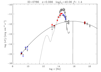
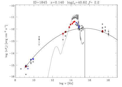
Figure 2: Examples of the SED of two LPBLs, namely ID=786 and ID=1845. We show data analyzed by us (colored symbols) as well as data downloaded from the ASDC (grey dots); see Fig. 10 for a full description. The near-IR, optical, and X-ray data have been corrected for Galactic absorption. We overplot the logarithmic parabolic fit through the data points at 1.4 GHz, $\rm 12\,\mu m$, rest-frame 3900 Å, and 1 keV (black empty circles), where the infrared and optical fluxes have been corrected for the host galaxy contribution. The grey line represents an elliptical galaxy template normalized to the W2 flux density.

Table 1: The 34 BL Lac objects identified by Capetti & Raiteri (2015) and their $k$-corrected luminosities in the various bands.

ID	R.A.	Dec.	$z$	$\log L_{\rm r}$	$\log L_{\rm i}$	$\log L_{\rm o}$	$\log L_{\rm x}$	$\log L_{\gamma}$	$\Gamma_{\gamma}$
	[deg]	[deg]		[$\>{\rm erg}\,{\rm s}^{-1}$]	[$\>{\rm erg}\,{\rm s}^{-1}$]	[$\>{\rm erg}\,{\rm s}^{-1}$]	[$\>{\rm erg}\,{\rm s}^{-1}$]	[$\>{\rm erg}\,{\rm s}^{-1}$]
507	118.654457	39.17994	0.096	40.20	42.99	43.56	42.85
786	193.445877	3.44177	0.066	40.06	42.82	43.31	43.07	43.00	1.84 (0.10)
1087	234.945602	3.47208	0.131	39.86	42.58	42.94	42.49
1103	164.657227	56.46977	0.143	41.23	44.26	44.58	43.95	44.42	1.95 (0.03)
1315	14.083661	$-$9.60826	0.103	40.58	43.39	43.68	43.89	43.22	1.79 (0.12)
1768	201.445267	5.41502	0.135	40.05	42.74	43.06	42.90
1805	119.060333	27.40993	0.140	40.17	42.73	42.86	$<$42.85
1845	163.433868	49.49889	0.140	40.62	43.44	43.77	43.43	43.53	1.80 (0.10)
1903	121.805740	34.49784	0.139	40.36	43.07	43.07	$<$42.89
1906	122.412010	34.92701	0.082	40.56	42.98	43.27	43.66	42.74	1.67 (0.13)
2061	119.695808	27.08766	0.099	40.34	43.46	43.26	$<$42.55	43.28	2.13 (0.12)
2083	132.650848	34.92296	0.145	40.39	43.29	43.78	43.31	43.25	1.92 (0.20)
2281	144.188004	5.15749	0.131	40.29	43.25	43.24	$<$42.82
2341	151.793533	50.39902	0.133	40.30	42.54	42.92	$<$42.59
2440	212.955994	52.81670	0.076	40.81	42.87	42.83	42.65	42.76	2.56 (0.23)
3091	216.876160	54.15659	0.106	40.06	43.15	42.97	42.81
3403	217.135864	42.67252	0.129	40.43	43.38	44.03	44.91	43.39	1.57 (0.09)
3591	172.926163	47.00241	0.126	40.87	42.88	43.14	42.94
3951	183.795746	7.53463	0.136	40.75	43.32	43.76	43.93
3958	185.383606	8.36228	0.132	40.98	42.72	43.29	43.45
4022	233.009293	30.27470	0.065	39.95	42.77	43.02	43.38	42.63	1.77 (0.13)
4156	196.580185	11.22771	0.086	40.48	42.75	42.73	$<$42.32
4601	199.005905	8.58712	0.051	39.19	42.28	42.37	$<$41.86
4756	229.690521	6.23225	0.102	40.89	43.13	43.60	44.00
5076	180.764603	60.52198	0.065	40.39	43.64	43.88	42.68	43.16	2.21 (0.08)
5997	127.270111	17.90440	0.089	40.81	42.95	43.22	43.30
6152	162.411652	27.70362	0.144	40.08	42.67	43.14	42.95
6428	169.276047	20.23538	0.138	40.92	43.66	44.20	45.01	44.03	1.87 (0.05)
6943	194.383087	24.21118	0.140	39.89	42.78	43.57	44.34
6982	212.616913	14.64450	0.144	41.53	43.41	43.57	42.79
7186	211.548355	22.31630	0.128	39.70	42.53	42.73	42.31
7223	223.784271	19.33760	0.115	39.73	42.80	42.91	43.46
9640	227.671326	33.58465	0.114	39.33	42.92	42.88	43.68
10537	233.696716	37.26515	0.143	40.23	43.19	43.90	42.87	43.54	2.11 (0.12)

Column description: (1) ID number; (2 and 3) coordinates in degrees; (4) redshift, $k$-corrected luminosity at (5) 5 GHz; (6) 12 $\mu$m; (7) 3900 Å; (8) 1 keV, (9) 1 Gev; 3FGL $\gamma$-ray spectral index (with error).

3.1 Radio

Our 34 LPBLs were selected from the sample of 18286 radio sources built by Best & Heckman (2012). We use radio data from the Faint Images of the Radio Sky at Twenty-cm (FIRST) survey. Therefore, our reference radio frequency is 1.4 GHz.

In general, there are many data available in the radio band. In particular, for 22 LPBLs the Green Bank survey (Gregory & Condon, 1991) provides information at 4.8 GHz. The average radio spectral index between 1.4 and 4.8 GHz is 0.02 with a standard deviation of 0.07. This confirms that we are dealing with objects with flat radio spectra, as expected for BL Lacs. The scatter of radio data for the same source is likely due to the jet emission variability and to different spatial resolution. Only a few objects have millimeter observations and these are not further considered.

3.2 Infrared

In the infrared we use the all-sky survey made by the WISE satellite (Wright et al., 2010), which provides magnitudes in the four filters W1 ($\rm 3.4\mu m$), W2 ($\rm 4.6\mu m$), W3 ($\rm 12\mu m$), and W4 ($\rm 22\mu m$). Cross-match with the AllWISE catalog was performed with a 3 arcsec radius (see Paper I, ).

We choose $\rm 12\mu m$ as the reference wavelength in the infrared to reduce the strong contamination by the host galaxy light and, at the same time, have accurate data. We calculate the host contribution at the W3 wavelength by normalizing the SWIRE template of a 13 Gyr old elliptical galaxy (Polletta et al., 2007) to the W2 value (see Fig. 2). This contribution is then subtracted to the AllWISE W3 flux density to get the jet emission at that wavelength. This correction is likely overestimated, since it assumes that the whole emission in W2 is from the host galaxy; however, it has a negligible effect on the W3 value because of the steep fall of the galaxy emission going toward the far infrared. Indeed, the host contribution in W3 is only about 1% of the jet contribution.

3.3 Optical

We calculate the jet flux density $F_{\rm o}$ at 3900 Å rest frame from the Dn(4000) values derived from the SDSS spectra by the group from the Max Planck Institute for Astrophysics and Johns Hopkins University (Brinchmann et al., 2004; Tremonti et al., 2004),

$$F_{\rm o}={\rm{D^{0}_{n}-Dn(4000)}\over{D^{0}_{n}-1}}F_{\rm SDSS}$$

where $F_{\rm SDSS}$ is the SDSS flux density at 3900 Å (reddening-corrected), and ${\rm D^{0}_{n}}$ is the Dn(4000) value for quiescent galaxies, which slightly changes with redshift (see Paper I, ).

3.4 X-rays

Most of our sources have X-ray flux measurements. In principle, these could also be affected by the emission from the host hot coronae. However, the LPBL X-ray luminosity usually exceeds those measured from the galactic components, which are generally smaller than $10^{42}$ $\>{\rm erg}\,{\rm s}^{-1}$ (Fabbiano et al., 1992).

Flux densities at 1 keV were derived from the ROSAT All Sky Survey (RASS), which provides the source count rate in the 0.1–2.4 keV energy range. Counts-to-flux conversion factors are given for three possible photon spectral indices $\Gamma_{\rm x}=1,2,3$. Adopting a search radius of 30 arcsec, we found seven sources in the RASS Faint Source Catalog and 17 in the Bright Source catalog (Voges et al., 1999). Since in general we do not know the spectral slope of each source, we consider all the three possibilities and correct for Galactic absorption using WebPIMMS. Figure 3 shows the ROSAT count rates corresponding to an un-absorbed flux of $10^{-11}\rm\,erg\,cm^{-2}\,s^{-1}$ as a function of $N_{\rm H}$ for the three spectral indices. The spread of the count rate due to different slopes is minimum for $\log N_{\rm H}=20.2$–20.3 [$\rm cm^{-2}$], and grows for both increasing and decreasing Galactic absorption. We fit the three relationships with fourth-order polynomial curves and apply them to find the de-absorbed flux corresponding to our LPBLs count rates.

For the following analysis, we use the 1 keV de-absorbed flux densities obtained with $\Gamma_{\rm x}=2$. However, given the distribution of column densities for our LPBLs, since all but one (ID=1103) of them is $20.0\lesssim\log N_{\rm H}\lesssim 20.7$ [$\rm cm^{-2}$], the flux measurements obtained by adopting $\Gamma_{\rm x}=1$ or 3 differ by at most 40% from the adopted values.

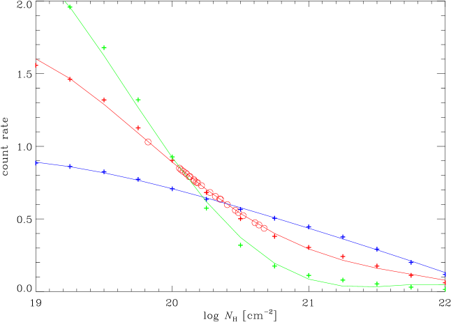
Figure 3: The ROSAT count rate corresponding to an unabsorbed flux of $10^{-11}\rm\,erg\,cm^{-2}\,s^{-1}$ versus the Galactic hydrogen column density $N_{\rm H}$ for the three values of the X-ray photon spectral index $\Gamma_{\rm x}=1$ (blue), 2 (red), and 3 (green). Plus signs indicate the values derived with WebPIMMS, and solid curves represent polynomial fits through them. Open circles correspond to the $N_{\rm H}$ values of our LPBLs.

For the ten sources lacking RASS data, we searched for observations with other X-ray satellites. We derive 1 keV flux densities of ID=3591 from the seven-year Swift-XRT point source catalog (1SWXRT; D’Elia et al., 2013). In the case of ID=7186, we use the 3XMM-DR5 catalog, containing source detections drawn from 13 years of XMM-Newton observations (Rosen et al., 2015). We use Chandra data reported by the ASDC for ID=1087.

Taking into account that the faintest LPBL in the RASS has a count rate of 0.025 counts/s, we assume an upper limit of 0.02 counts/s for the remaining seven sources without X-ray detection. This corresponds to a flux of $1.12\,10^{-13}\,\rm erg\,cm^{-2}\,s^{-1}$ for a $\Gamma_{\rm x}=2$ spectral index, and implies 6–10 counts for typical exposure times of 300–500 s. The actual flux upper limits are obtained by correcting the limit to the count rate for Galactic absorption toward each individual source.

3.5 $\gamma$-rays

The Fermi Large Area Telescope Third Source Catalog (3FGL; Acero et al., 2015) includes the first four years of data from the mission. We found 13 Fermi counterparts to our objects, up to a maximum distance of $\sim 400$ arcsec. In the catalog, the spectra of all these objects have been fitted with a power law, which is plotted in the SEDs reported in the Appendix with its uncertainties on both the flux and spectral index (giving rise to a “butterfly”). According to the 3FGL, only one object, ID=3403, has a possible association with a TeV source.

In summary, to analyze the jet emission in LPBLs, we can rely on data in the radio, mid-infrared, optical, X rays (for most of them), and $\gamma$ rays (for some of them).

Even if all objects span a small range of redshift, we need to perform $k$-correction to derive rest-frame luminosities (see Table 1) and colors. When $k$-correcting (or transforming flux densities from one frequency to another inside the same band), we need spectral indices. In the radio we assume $\alpha_{\rm r}=0$, while at $\gamma$ rays we use the specific index of each source. In more detail, to calculate the rest-frame 1 GeV luminosity $L_{\gamma}$ reported in Table 1, we transformed the flux density at the pivot energy (energy at which the error is minimum) into flux density at 1 GeV and then $k$-corrected, in both cases, with the specific spectral index of each source given in the 3FGL. For the other bands we follow F98. Since we do not know a priori what type of BL Lac objects we are dealing with, we use average values between those corresponding to the Slew and 1 Jy samples, namely, $\alpha_{\rm i}=0.70$, $\alpha_{\rm o}=0.94$, $\alpha_{\rm x}=1.325$. We stress that because of the limited range of redshift of the LPBLs sample, the corrections are very small and the precise values adopted do not affect significantly our analysis.

4 The nature of LPBLs

One useful quantity to establish the flavor of BL Lacs is the ratio of the X-ray to radio fluxes. As mentioned in the Introduction, according to Padovani & Giommi (1995) and Bonnoli et al. (2015), this ratio should be greater than 200 and 10000 to define an HBL and EHBL, respectively. Equivalently, F98 defined HBL as those objects with $\alpha_{\rm rx}\la 0.75$, where the LBL has $\alpha_{\rm rx}\ga 0.75$.

We calculate broadband spectral indices for our LPBLs after dereddening and $k$-correction. To ease the comparison with previous results, radio fluxes were converted from 1.4 to 5 GHz and optical fluxes from 3900 to 5500 Å.

In Table 2 we list the ratio of the X-ray to the radio luminosity and the radio-X-ray spectral index. Based on these parameters, which give the same indication, seven objects are LBL, 19 are HBL, and four are EHBL. For the remaining four objects, all without an X-ray detection, the resulting lower limit on $\alpha_{\rm rx}$ does not lead to a secure classification.

As mentioned in the Introduction, we are dealing with sources whose flux is variable at all wavelengths with timescales ranging from minutes to months. We are using catalog data, which are not taken simultaneously, and this may cause some distortion of the SED. However, while the individual classifications must be taken with some caution, we do not expect that variability can alter the conclusions drawn from a sizeable sample of objects.

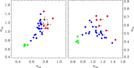
Figure 4: Broadband spectral indices for the objects in our LPBL sample, separating LBL (red circles) from HBL (blue diamonds) and EHBL (green squares)

In Fig. 4 we show the optical-X-ray versus radio-X-ray and the radio-optical versus optical-X-ray spectral indices for the three BL Lac classes. They are in good agreement with the results obtained by Donato et al. (2001), because the different BL Lac classes cover the same range of values. The positive dependence of $\alpha_{\rm ox}$ on $\alpha_{\rm rx}$ is a signature of the SED curvature that increases from EHBL toward LBL. This effect can be studied in a more quantitative way by reproducing the SEDs with a log-parabolic model.

In Fig. 5 we show the radio, infrared, optical, X-ray, and $\gamma$-ray luminosities of our LPBLs (see Table 1). The radio–X-ray SEDs are fitted with a log-parabolic curve, whose apex roughly represents the synchrotron peak. Although in principle this should be determined through a synchrotron emission model, the uncertainty derived from the choice of the model parameters makes a simple parabolic fit equally valid for our purposes. In the lower panel, luminosities in the various bands are plotted as a function of the synchrotron peak frequency $\nu_{\rm peak}$. There is no significant trend of $\nu_{\rm peak}$ with $L_{\rm r}$, $L_{\rm i}$, or $L_{\rm o}$. Conversely, $\nu_{\rm peak}$ clearly increases with $L_{\rm x}$. This is the natural consequence of the large spread in the X-ray luminosities of the various BL Lac classes.

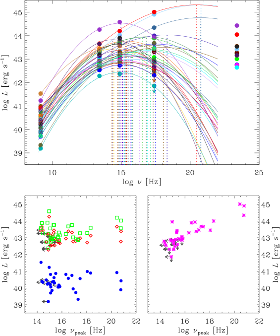
Figure 5: Upper panel: radio-to-$\gamma$-ray SEDs for the 34 objects analyzed in this paper (colored dots). Solid lines represent parabolic fits to the radio–X-ray data. Vertical dotted lines identify the parabola apices, which give an indication of the synchrotron peak position. For the objects without X-ray detection, the peak location should be considered an upper limit. Lower panels: luminosities versus the synchrotron peak frequency. Blue dots, red diamonds, green squares, and pink asterisks refer to radio, infrared, optical, and X-ray bands, respectively. In all panels, upper limits due to the lack of detection in the X-ray band are indicated with arrows.

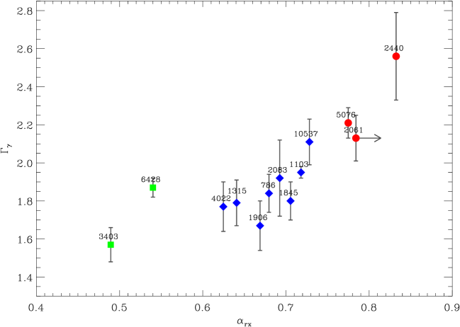
Figure 6: $\gamma$-ray photon spectral index $\Gamma_{\gamma}$ versus the radio-X-ray energy spectral index $\alpha_{\rm rx}$. Red dots represent LBL, blue diamonds HBL, and green squares EHBL.

Our estimate of the synchrotron peak frequency ranges from $\log\nu=14.3$ to 20.8 (see Table 2), i.e., from the infrared to hard X-rays, confirming that the sample includes both LBL as well as HBL and EHBL. For the sources not detected in X-rays, the peak location must be considered as an upper limit. By adopting $\log\nu_{\rm peak}=15$ as a dividing value between LBL and HBL, overall we recover a classification in concordance with that based on the X-rays/radio comparison. There are only three exceptions (indicated with an asterisk in Table 2). For these objects we look for further data that can constrain their nature. The X-ray spectrum of ID=3591 is soft (XRT data from the ASDC) and this would define it as an HBL. We have $\gamma$-ray information from Fermi for the other two objects. In Figure 6 we plot $\Gamma_{\gamma}$ versus $\alpha_{\rm rx}$, highlighting the various BL Lac classes. As expected, $\Gamma_{\gamma}$ increases with $\alpha_{\rm rx}$ and all HBL have $\Gamma_{\gamma}<2$ but one, ID=10537, whose nature thus remains unclear. The LBL definition of ID=2440 is instead confirmed by its very soft $\gamma$-ray spectrum. Furthermore, for two LPBLs not classified with the X-rays/radio method, the peak location suggests a definition as LBL (these objects are denoted as “LBL?” in Table 2).

However, in LBLs the X-ray emission is generally dominated by the inverse-Compton contribution. Therefore, a fit to the synchrotron bump including the X-ray emission overestimates $\nu_{\rm peak}$. We tested the relevance of this effect by fitting the radio-to-optical SED of our sources, and indeed we found that in some cases the three-point fit gives a $\nu_{\rm peak}$ that is significantly lower than the four-point fit, and as low as $\log\nu_{\rm peak}\sim 13.5$ (see Fig. 7). In particular, the $\nu_{\rm peak}$ shift is significant for most objects without an X-ray detection and, in general, means that the four-point fit overestimates the synchrotron contribution to the X-ray flux.

At the opposite end of the $\nu_{\rm peak}$ distribution, we obtained formal values as high as 10^20.8 Hz for the EHBLs, which are not well constrained by the available measurements,however. In two of such sources the SED shown in the Appendix suggests a peak location between $10^{18}$–$10^{19}$ Hz.

BL Lacs drawn from flux limited radio samples are known to include mostly LBL (e.g., Padovani et al., 2003). Conversely, the LPBL sample considered here, although initially selected in the radio band, is biased against the selection of LBL. Indeed, one of the requirements is a significant dilution of the host emission by the nonthermal emission across the Ca II break; sources peaking at low energies, well before the optical band, are less likely to be selected. Indeed, as shown by Fig. 15 in Paper I, the selection function of LPBL has a cut-off at a luminosity that shifts toward a higher power when $\alpha_{\rm ro}$ increases, thus disfavoring the detection of LBL with respect to HBL.

In summary, our classification of LPBLs in their different flavors shows that while the bulk of our LPBL sample is formed by HBLs (or EHBLs), despite the negative bias in our sample about one quarter of them are LBLs.

According to F98, all the sources with $\log L_{\rm r}<42$ at 5 GHz have $\log\nu_{\rm peak}>15.5$. When correcting for the difference in cosmology, the above luminosity limit translates into $\log L_{\rm r}<41.2$ at 1.4 GHz. All our LPBLs but two fulfill this requirement, but they are characterized by peak frequencies that, for the objects that lack an X-ray detection, may reach $\log\nu_{\rm peak}\sim 13.5$. We recall that Padovani et al. (2003) found six BL Lacs under the above luminosity limit with peak frequencies extending down to $\sim 10^{13}\rm\,Hz$ and seven were found by Antón & Browne (2005) down to $\sim 10^{14}\rm\,Hz$. In both cases, the minimum 1.4 GHz luminosity of the objects is $\log L_{\rm r}\sim 40.2$, so our analysis confirms and extends the results of these previous studies to lower luminosities.

Table 2: Classification of the LPBLs into the various BL Lacs groups based on the ratio between X-ray to radio luminosities or, equivalently, to the radio-X-ray spectral index. We also report the synchrotron peak frequency obtained from a log-parabolic fit to the $k$-corrected radio, infrared, optical, and X-ray luminosities. Objects with discordant classification are indicated with an asterisk. Notes on individual sources are given in the Appendix.

ID	$L_{\rm x}/L_{\rm r}$	$\alpha_{\rm rx}$	$\nu_{\rm peak}$	Class	Notes
507	445	0.73	15.1	HBL	Y
786	1036	0.68	15.8	HBL	Y
1087	426	0.73	15.2	HBL
1103	524	0.72	15.0	HBL	Y
1315	2061	0.64	16.5	HBL	Y
1768	701	0.70	15.7	HBL
1805	$<$482	$>$0.72	$<$15.8	?
1845	654	0.71	15.4	HBL	Y
1903	$<$341	$>$0.74	$<$15.2	?
1906	1251	0.67	17.5	HBL	Y
2061	$<$163	$>$0.78	$<$14.5	LBL	Y
2083	823	0.69	15.3	HBL
2281	$<$336	$>$0.74	$<$14.9	LBL?	Y
2341	$<$194	$>$0.77	$<$15.4	LBL
2440	69	0.83	15.1	LBL*	Y
3091	561	0.71	15.1	HBL	Y
3403	29999	0.49	20.8	EHBL	Y
3591	117	0.80	15.5	LBL*	Y
3951	1520	0.66	16.8	HBL
3958	294	0.75	18.1	HBL
4022	2733	0.62	16.9	HBL	Y
4156	$<$ 69	$>$0.83	$<$14.7	LBL	Y
4601	$<$468	$>$0.72	$<$14.9	LBL?	Y
4756	1271	0.67	18.3	HBL	Y
5076	192	0.77	14.4	LBL	Y
5997	305	0.75	16.3	HBL
6152	732	0.70	15.8	HBL
6428	12207	0.54	20.4	EHBL	Y
6943	28108	0.49	20.8	EHBL	Y
6982	18	0.91	14.3	LBL
7186	404	0.73	15.1	HBL	Y
7223	5415	0.59	17.1	HBL
9640	22528	0.51	17.3	EHBL	Y
10537	438	0.73	14.8	HBL*	Y

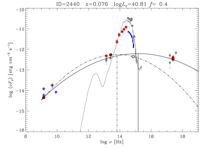
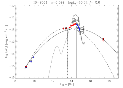
Figure 7: Examples of the SED of two LPBLs, namely ID=2440 and ID=2061. The solid line represents a logarithmic parabolic fit, including the radio, infrared, optical, and X-ray data points, which does not match the infrared and optical data. These are instead well reproduced by a 3-point fit excluding the X-ray datum (dot-dashed line). The case shown in the left panel indicates that the X-ray emission is likely dominated by the inverse-Compton component; that in the right panel highlights how the upper limit to the X-ray flux leads to a large overestimate of the synchrotron peak frequency. The grey line represents an elliptical galaxy template normalized in W2 and the grey dots show data collected from the ASDC.

5 The blazar sequence

As mentioned in the Introduction, F98 identified a continuous trend of the blazar SEDs, where BL Lacs of lower radio power exhibit higher synchrotron and inverse-Compton peak frequencies and lower Compton dominance with respect to the higher power objects. In their work, the faintest SED has a median 5 GHz luminosity of $\log L_{\rm r}=40.97$, and according to their model the peak synchrotron frequency is around $\log\nu=16.5$ [Hz]. Subsequently, Donato et al. (2001) added a hard X-ray point to the F98 SEDs and slightly modified the model, so that the peak frequency of the faintest SED shifted to $\log\nu\sim 16$. If instead we fit their radio-to-hard-X points with a simple log-parabolic curve, we get a peak frequency of $\log\nu=16.2$. The data points of the faintest three SED in these works are plotted in Fig. 8 and some of their properties are reported in Table 3.

Following F98 we consider the median luminosities in the various bands of all 34 LPBLs, obtaining the values tabulated in Table 3 and plotted in Fig. 8. Building median SEDs has the advantage of reducing the effects of variability when nonsimultaneous data are used.

The presence of upper limits to the X-ray fluxes does not affect the estimate of the median luminosity in this band because they are all located within the faintest half of the distribution. For this reason, the median is well defined. The radio luminosity of the faintest median SED in F98 and Donato et al. (2001) is similar to that of our sample of LPBLs. However, the two SEDs diverge at increasing frequencies, reaching a difference of a factor $\sim 40$ at 1 keV. Indeed, a log-parabolic fit gives a peak frequency at $\log\nu=15.3$ for the LPBLs, which is substantially lower than that found by F98 and Donato et al. This highlights that our sample is very different from that of the faintest objects analyzed by F98 because it includes a much higher fraction of LBLs.

We can further split our sample into groups of radio luminosity. We define two subsamples of equal size. The median luminosities are reported in Table 3 and shown in Fig. 8. The median $\gamma$-ray luminosity is only defined for the brighter sample. There are no significant differences in both shape and peak frequency between these two SEDs, despite the difference in radio luminosity. Moreover, the corresponding $\nu_{\rm peak}$ lies in between the peaks of the two least luminous groups considered by F98. Apparently, the trend of increasing $\nu_{\rm peak}$ at decreasing $\log L_{\rm r}$ does not apply to the least luminous BL Lacs.

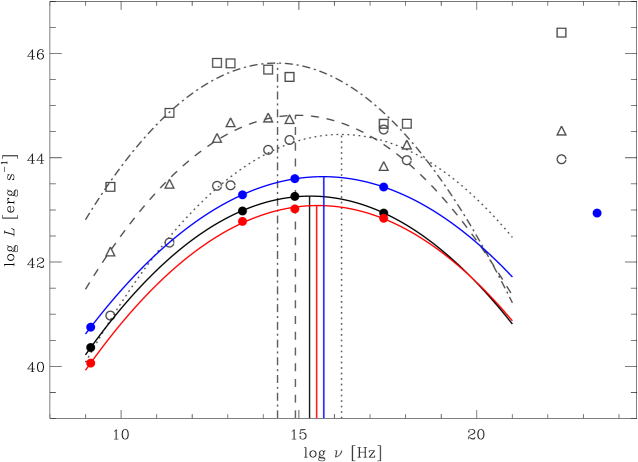
Figure 8: Median SED for the 34 objects analyzed in this paper (black dots). The red and blue dots represent the SEDs obtained by splitting the sample into two groups of increasing radio luminosities (see text and Tab. 3). Gray symbols refer to the SEDs of the three faintest subsamples in the F98 work, complemented by the hard X-ray data points from Donato et al. (2001). The curves are log-parabolic fits to the radio-to-X-ray median luminosities with the peak indicated with vertical lines.

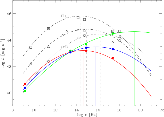
Figure 9: The same as Fig. 8, but now different colors refer to the three flavors of BL Lac objects (red=LBL, blue=HBL, green=EHBL).

Because of the different flavor of BL Lacs in our sample, the above described median SEDs are the result of a mixture of sources with different properties. Therefore, we calculate the median SEDs for LBL, HBL, and EHBL separately. The result is shown in Fig. 9, where the parabolic fits are made through the radio-to-X-ray data for the HBL and EHBL cases, while for the LBL we do not consider the X-ray point for the above discussed reasons. Aside from the obvious shift of $\nu_{\rm peak}$, there are two notable features. The first is the small difference in radio luminosity among the three classes, where LBL (EHBL) are only a factor of two brighter (fainter) than HBL. The second is the similarity of our LBL SED shape with that of the LBL in F98, which have radio luminosities 30–600 times higher.

Table 3: Properties of the median BL Lacs SED

Selection	$N$	$\log L_{\rm 5GHz}$	$\log L_{\rm 1keV}$	$\log\nu_{\rm peak}$
Fossati et al. 1998
$\log L_{\rm r}=43$–44	17	43.44	44.65	14.4
$\log L_{\rm r}=42$–43	10	42.20	43.84	14.9
$\log L_{\rm r}<42$	38	40.97	44.54	16.2
This work
all	34	40.91	42.94	15.3
$\log L_{\rm r}>40.9$	17	41.30	43.44	15.7
$\log L_{\rm r}<40.9$	17	40.61	42.84	15.5
LBL	7	40.67	42.64	14.6
HBL	19	40.38	43.31	15.8
EHBL	4	40.14	44.48	19.4

Column description: (1) Group description, (2) number of objects in the radio band, (3) and (4) median radio and X-rays luminosities, (4) synchrotron peak frequency.

6 The beaming effect

Up to now we have not considered the fact that blazars are beamed sources with their luminosities enhanced by relativistic Doppler boosting, which also blueshifts the synchrotron peak frequency. The relationship between the emitted luminosities $L^{\prime}$ and their beamed counterparts is $L=\delta^{4}\,L^{\prime}$, where $\delta$ is the Doppler factor. Analogously, the frequencies transform as $\nu=\delta\,\nu^{\prime}$.

Nieppola et al. (2008) considered Doppler factors derived from the study of the total flux density variability and found that they anticorrelate with the peak frequency. These authors suggested that the anticorrelation between $L_{\rm r}$ and $\nu_{\rm peak}$ becomes a positive correlation when correcting for beaming. Nieppola et al. (2008) used Doppler factors inferred from the analysis of radio data. However, the jet radiation at different frequencies is likely emitted from different regions along the jet, each with its own Doppler factor. Indeed, the usually long (weeks to months) delay of the radio variations after the higher energy variations (in particular optical and $\gamma$-ray), and the longer radio variability timescales (e.g., Raiteri et al., 2008; Villata et al., 2009) suggest that the radio emission comes from a more external and extended jet zone than that producing the high-frequency synchrotron radiation. Taking into account that the Doppler factor $\delta$ depends on both the bulk Lorentz factor and the viewing angle, accelerating/decelerating processes and/or bends in the jet structure (e.g., Lister, 2001; Lister et al., 2013) would cause a spread of $\delta$ values within the same source in different bands. In turn, this would produce a distortion of the observed SED shape with respect to the intrinsic SED shape.

7 Summary and conclusions

We explored the properties of the SED of a complete sample of 34 BL Lacs of low power. These objects have been selected in the redshift range $0.05<z<0.15$ in Paper I based on a new diagnostic plane that includes the W2$-$W3 color from WISE and the Dn(4000) index derived from the SDSS.

We collected multiwavelength data focusing on those bands that allow us to study the jet emission. We have a complete coverage at the frequencies used for the sample selection (1.4 GHz, 12 $\mu$m, and rest-frame 3900 Å). X-ray fluxes are available for most of the sources (27 out of 34), while only 13 of them are detected at $\gamma$-rays.

We classified the LPBL based on the ratio between radio and X-rays luminosities or, equivalently, on the radio-X-ray spectral index, finding that seven of them are LBL, 19 are HBL, and four are EHBL. The lack of X-rays data prevent us from obtaining a robust classification for the last four objects.

We derived an estimate of the synchrotron peak frequency from each SED through a log-parabolic fit to the $k$-corrected jet luminosities. Overall, the mix of BL Lac types is confirmed by the location of the peak frequency, ranging from $\log\nu=14.3$ to 20.8, i.e., from the infrared to the hard X-rays. However, the SEDs of some LPBLs are better described by a three-point fit (excluding the X-ray data). For these sources, the peak frequency shifts at much lower energies, as low as $\log\nu_{\rm peak}\sim 13.5$, which implies that the X-ray emission also receives a contribution from the inverse-Compton process, as expected in LBLs. LPBLs with synchrotron peaks located at even lower energies would be very difficult to find with our method. Indeed, the nonthermal contribution to the optical flux might be insufficient to lower the Dn(4000) and the lines EW might not be significantly reduced with respect to the parent population.

We estimated the median SED for the sample as a whole and for two subsamples based on different thresholds of radio luminosity. The advantage of this approach is to mitigate the effects of variability when nonsimultaneous data are used, as in our case. We found that the peak frequencies obtained with such an analysis all fall at $\log\nu_{\rm peak}\sim 15.5$ Hz. These values are lower than that characterizing the least luminous group of BL Lacs considered by F98 that have similar radio luminosity of our LPBLs. In our sample, the sources classified as LBL, HBL, or EHBL do not differ significantly in radio luminosity. The peak frequency of the median SED of LBLs is located at $\log\nu_{\rm peak}\sim 14.6$, consistent with the value derived by F98 for much more luminous BL Lacs.

Apparently, there is no clear connection between the SED shape and the radio power within the LPBL sample. At least at low luminosity, BL Lacs do not populate any preferred region in the $\log L_{\rm r}$ versus $\nu_{\rm peak}$ plane and the trend of increasing $\nu_{\rm peak}$ at decreasing $L_{\rm r}$ does not extend to the least luminous BL Lacs. The reason is the presence of a significant fraction of LBL objects. This is remarkable when considering that our LPBL sample is biased against the selection of LBLs.

Furthermore, the SED of the LBLs included in our sample is very similar to that of radio-selected BL Lacs that are up to two-three orders of magnitude more luminous. These results cast serious doubts on the idea that the radio luminosity is the main driving parameter of the multiwavelength properties of BL Lacs.

In contrast, there is a clear positive dependence of $\nu_{\rm peak}$ on $\log L_{\rm x}$. This implies that X-ray flux-limited samples necessarily lead to the selection of objects with synchrotron peaks at higher energies. Previous works had already suggested that the blazar sequence is an artifact due to biases in the samples used by F98. The present analysis confirms this result with a much larger sample of LPBLs reaching luminosities one order of magnitude lower.

Finally, the shape of the intrinsic SED can be distorted by relativistic beaming in case there are accelerating/decelerating processes in the jet and/or bends in the jet structure. This suggests caution in interpreting the observed spread in the spectral behavior of BL Lacs.

Appendix A Spectral energy distributions

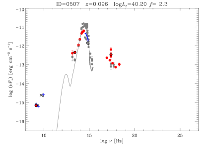
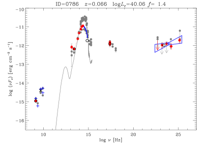
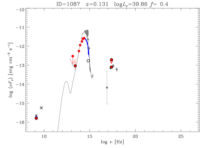
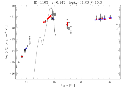
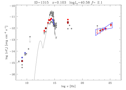
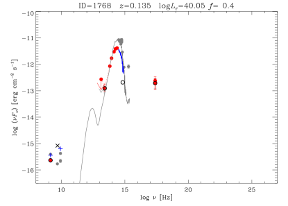
Figure 10: Broad-band SEDs of the 34 LPBLs analysed in this paper. Red dots represent flux densities derived from the FIRST, AllWISE, 2MASS, RASS, 3XMM, and 3FGL catalogs. Blue plus signs show other radio data and the $\gamma$-ray flux density at the pivot energy; the black crosses represent the 1.4 GHz FIRST data converted into 5 GHz ones with $\alpha_{\rm r}=0$. The SDSS spectrum and the Fermi power-law fit butterfly are plotted in blue. Near-infrared, optical, and X-ray data have been corrected for Galactic absorption. The black circles highlight the reference radio (1.4 GHz), infrared (W3 band), optical (3900 Å rest-frame), X-ray (1 keV), and $\gamma$-ray (1 GeV) jet flux densities. In the W3 band, the jet flux density has been corrected for the host contamination estimated from an elliptical galaxy template (grey line) normalized in the W2 band. In the optical, the jet contribution has been derived from the Dn(4000). Grey dots show data downloaded from the ASDC.

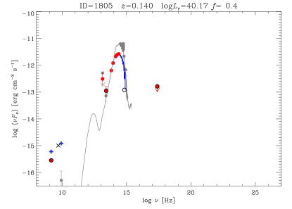
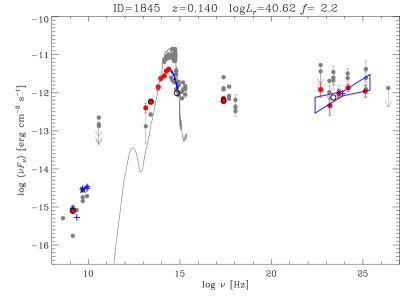
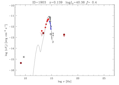
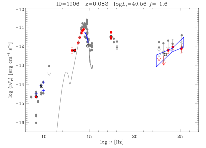
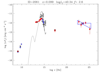
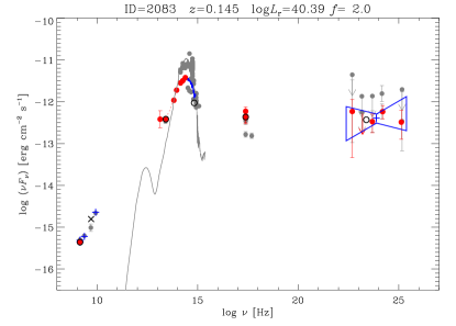
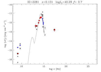
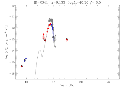
Figure 10: (continued)

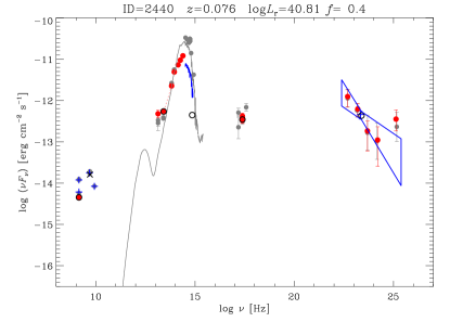
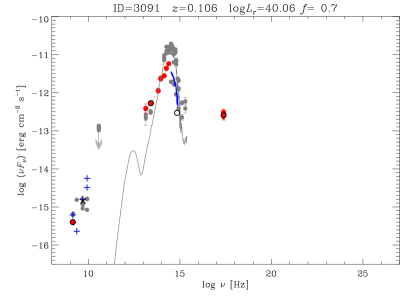
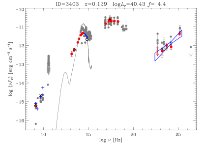
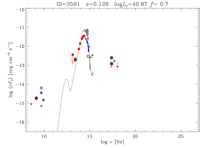
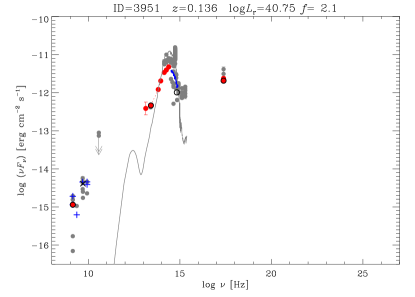
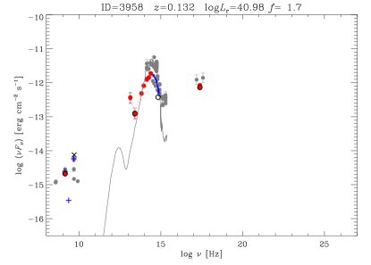
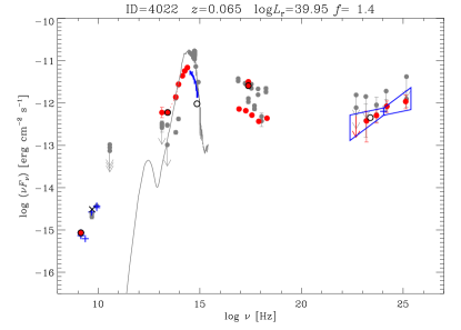
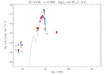
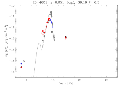
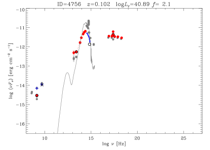
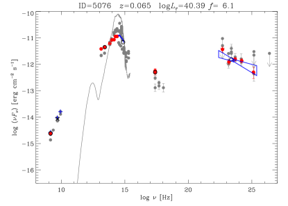
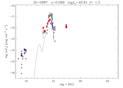
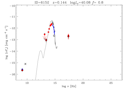
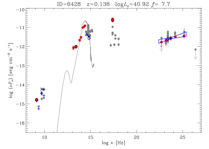
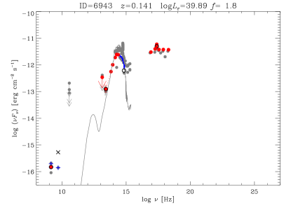
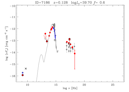
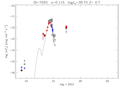
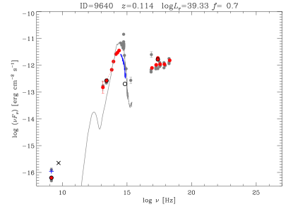
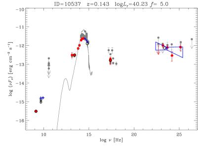
Figure 10: (continued)

In Figure 10, we show the broadband SEDs of our sources. They contain the FIRST as well as other radio data (NVSS; Green Bank, VLBI); the AllWISE flux densities in the W1, W2, W3, and W4 bands, the $J,H,K$ flux densities from the 2MASS; the SDSS spectrum; the RASS and 3XMM X-ray data, and the 3FGL $\gamma$-ray fluxes. The near-infrared, optical, and X-ray data have been corrected for Galactic absorption.

The RASS 0.1–2.4 fluxes have been converted into 1 keV flux densities with all the three possible spectral indices $\Gamma_{\rm x}=1,2,3$ to quantify the uncertainties. At $\gamma$ rays, we show the 3FGL data for the various energy bins, the flux density at the pivot energy, and the butterfly resulting from the power-law spectral fit.

We also highlight the reference radio (1.4 GHz), infrared (W3 band), optical (3900 Å rest-frame), X-ray (1 keV), and $\gamma$-ray (1 GeV) jet flux densities (see Section 3). In the W3 band, the jet flux has been corrected for the host contamination estimated from an elliptical galaxy template normalized in the W2 band. The optical jet emission has been derived from the Dn(4000). For the sources for which no RASS detection was available, we give upper limits obtained by assuming a ROSAT count rate of 0.02 counts/sec. The 1 GeV flux density was obtained from the flux density at the pivot energy. We also plot data downloaded from the ASDC.

A.1 Notes on individual sources

ID=507

The soft X-ray spectrum from XMM-Newton confirms its HBL nature.

ID=786

Its HBL flavor is verified by the soft X-ray and hard $\gamma$-ray spectra.

ID=1103

The soft X-ray and mildly hard $\gamma$-ray spectra agree with an HBL classification.

ID=1315

Its HBL nature is confirmed by the soft X-ray and hard $\gamma$-ray spectra.

ID=1845

Its HBL flavor is verified by the soft X-ray and hard $\gamma$-ray spectra.

ID=1906

Its HBL nature is confirmed by the soft X-ray and hard $\gamma$-ray spectra.

ID=2061

LBL with no detection in X-rays. With respect to the four-point fit to the SED, the three-point fit shifts $\log\nu_{\rm peak}$ from $<14.5$ to $13.7$.

ID=2281

LBL with no detection in X-rays; $\log\nu_{\rm peak}$ decreases from $<14.9$ to 14.1, changing the SED fit from four to three points.

ID=2440

Its LBL definition is confirmed by its hard X-ray and soft $\gamma$-ray spectra, which also suggests a Compton dominance. Indeed, $\log\nu_{\rm peak}$ goes from $<15.1$ in the four-point fit to the SED to 14.0 in the three-point fit.

ID=3091

We classified it as HBL, however, $\log\nu_{\rm peak}$ shifts from $15.1$ in a four-point to $13.7$ in a three-point SED fit. It may be that the SDSS spectrum met the source in a particularly low optical state.

ID=3403

This is the famous EHBL 1ES 1426+426, which has been extensively studied in X-rays. Indeed, its SED reveals an extremely bright X-ray flux and an exceptionally hard $\gamma$-ray spectrum, clearly identifying the source as an EHBL. The value $\log\nu_{\rm peak}=20.8$ we found is clearly overestimated; the XMM-Newton and ASDC data allow us to position it at $\log\nu_{\rm peak}\sim 17$–18.

ID=3591

Its LBL classification based on the radio and X-ray brightness is contradicted by the high synchrotron peak frequency as well as a soft X-ray (XRT) and a flat UV (UVOT+GALEX) spectrum (ASDC data). The 5 GHz flux density calculated from its 1.4 GHz FIRST value adopting $\alpha_{\rm r}=0$ is much higher than the other radio data, so that the wrong LBL definition is likely due to an underestimate of its $L_{\rm x}/L_{\rm r}$ and overestimate of its $\alpha_{\rm rx}$.

ID=4022

Its HBL nature is confirmed by the high X-ray flux with a soft X-ray and a hard $\gamma$-ray spectrum.

ID=4156

LBL without X-ray detection with $\log\nu_{\rm peak}$ shifting from $<14.7$ in a four-point to 14.1 in a three-point SED fit.

ID=4601

LBL without X-ray detection, with $\log\nu_{\rm peak}$ decreasing from $<14.9$ to 14.4 when changing the SED fit from four to three points.

ID=4756

The soft X-ray spectrum from XMM-Newton agrees with its HBL classification.

ID=5076

Its LBL flavor is confirmed by the low X-ray flux compared to the infrared and optical fluxes and by its soft $\gamma$-ray spectrum.

ID=6428

EHBL with a clearly overestimated $\log\nu_{\rm peak}=20.4$. The ASDC data show that its X-ray flux is extremely variable and that ROSAT found the source in a very bright state. Nonetheless, when considering the other X-ray data also, the source still appears as an HBL, which is proved by the mildly hard $\gamma$-ray spectrum.

ID=6943

EHBL with a clearly overestimated $\log\nu_{\rm peak}=20.8$. The XMM-Newton data confirm the X-ray brightness given by the RASS and add spectral information in favor of its EHBL nature, suggesting a $\log\nu_{\rm peak}$ of 17–18.

ID=7186

Its HBL classification is strengthened by the soft XMM-Newton X-ray spectrum.

ID=9640

A high X-ray state compared to the infrared and optical states, coupled with the hard X-ray spectrum detected by XMM-Newton, confirm its EHBL nature and suggest that the synchrotron peak falls at $\log\nu>18$.

ID=10537

The flavor of this BL Lac is difficult to assess. Both the four-point and three-point SED fits fail to give a satisfactory reproduction of the data. The high optical flux suggests an HBL classification, which is supported by a possible soft X-ray spectrum, but contradicted by the mildly soft $\gamma$-ray spectrum.

Figure 10: (continued)

Figure 10: (continued)