[7]G^ #1,#2_#3,#4(#5 #6— #7)

Quantum breaking of ergodicity in semi-classical charge transfer dynamics

Abstract

Does electron transfer (ET) kinetics within a single-electron trajectory description always coincide with the ensemble description? This fundamental question of ergodic behavior is scrutinized within a very basic semi-classical curve-crossing problem of quantum Landau-Zener tunneling between two electronic states with overdamped classical reaction coordinate. It is shown that in the limit of non-adiabatic electron transfer (weak tunneling) well-described by the Marcus-Levich-Dogonadze (MLD) rate the answer is yes. However, in the limit of the so-called solvent-controlled adiabatic electron transfer a profound breaking of ergodicity occurs. The ensemble survival probability remains nearly exponential with the inverse rate given by the sum of the adiabatic curve crossing (Kramers) time and inverse MLD rate. However, near to adiabatic regime, the single-electron survival probability is clearly non-exponential but possesses an exponential tail which agrees well with the ensemble description. Paradoxically, the mean transfer time in this classical on the ensemble level regime is well described by the inverse of nonadiabatic quantum tunneling rate on a single particle level.

Discovery of ergodicity breaking on the level of single molecular stochastic dynamics Barkai calls for re-examination of the basic models of stochastic transport in condensed matter. Even some standard models like diffusion in Gaussian disordered potentials with short-range correlations Zwanzig ; HTB90 can be mesoscopically non-ergodic PRL14 . This work discovers ergodicity breaking in another very popular and basic transport model based on a curve-crossing tunneling problem Nitzan . It is fundamental for quantum transport in condensed matter with a famous Landau-Zener-Stückelberg (LZS) result for the probability of quantum transitions LZS ; Nitzan

$$P_{\rm LZ}(v)=1-\exp\left[-f(v)\right]$$ (1)

between two diabatic quantum states $|1\rangle$ and $|2\rangle$, presenting a milestone. Here,

$$f(v)=\frac{2\pi}{\hbar}\frac{|V_{\rm tun}|^{2}}{|(\partial\Delta E(x))/\partial x)v|_{x=x_{*}}},$$ (2)

$v=\dot{x}$, is the result of the lowest second order quantum perturbation theory in the tunnel coupling $V_{\rm tun}$. It follows from the Fermi Golden Rule quantum transition rate

$$\Gamma(x)=\frac{2\pi}{\hbar}|V_{\rm tun}|^{2}\delta(\Delta E(x))$$ (3)

applied at the level crossing point $x^{*}$, $\Delta E(x^{*})=0$. $\Delta E(x)=E_{1}(x)-E_{2}(x)$ is the difference of the diabatic energy levels, which depends on time via a modulation parameter $x(t)$, $\delta(x)$ is the Dirac’s delta-function. Quantum system is characterized by the Hamiltonian $\hat{H}(x)=E_{1}(x)|1\rangle\langle 1|+E_{2}(x)|2\rangle\langle 2|+V_{\rm tun}(|1\rangle\langle 2|+|2\rangle\langle 1|)$, and the parameter $x(t)$ here is the nuclear coordinate, see in Fig. 1, which is treated classically (a mixed quantum-classical description), and $|i\rangle$, $i=1,2$ are two localized electronic states between which electron can tunnel. Within the Born-Oppenheimer approximation, $E_{1,2}(x)$ present diabatic energy potentials for $x(t)$. Furthermore, within the harmonic approximation and assuming that no nuclear frequency change occurs at electronic transitions, $E_{i}(x)=\kappa(x-x_{0}\delta_{2,i})^{2}/2-\epsilon_{0}\delta_{2,i}$. Then, $\Delta E(x)=\epsilon_{0}-\lambda+2\lambda x/x_{0}$, where $\epsilon_{0}$ is the difference of electron energy levels for equilibrium nuclei, $x_{0}$ is the reaction coordinate shift, and $\lambda=\kappa x_{0}^{2}/2$ is nuclear reorganization energy. Notice that electron tunnel distance has anything in common with $x_{0}$. Electron tunnels in space once the transition $|1\rangle\to|2\rangle$, or $|2\rangle\to|1\rangle$ takes place. Likewise, blinking of a quantum dot occurs once it is in the light emitting quantum state. Depending on the coupling strength $V_{\rm tun}$ and the velocity $v=\dot{x}$ at the the crossing point $P_{\rm LZ}(v)$ can vary from $P_{\rm LZ}(v)\approx f(v)\propto|V_{\rm tun}|^{2}/|v|$ (nonadiabatic transition) to one (adiabatic transition).

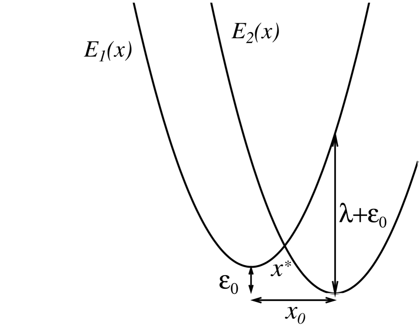
Figure 1: Curve crossing problem in the case of two equal potential curvatures $\kappa$ (i.e. no nuclear frequency change occurs at electronic transitions). Diabatic electron energy levels $E_{1,2}(x)$ provide harmonic potentials for the nuclear or molecular reaction coordinate $x$. $x_{0}$ is the nuclear equilibrium shift for different electron energies, and $\epsilon_{0}$ is the corresponding electron energy difference. $\lambda=\kappa x_{0}^{2}/2$ is nuclear (molecular) reorganization energy.

Within a classical treatment of the reaction coordinate $x$, one considers it as a particle of mass $M$ subjected to viscous frictional force $\eta v$, with a friction coefficient $\eta$, and zero-mean white Gaussian thermal noise of the environment $\xi(t)$ at temperature $T$. The friction and noise are related by the fluctuation-dissipation relation $\langle\xi(t)\xi(t^{\prime})\rangle=2k_{B}T\eta\delta(t-t^{\prime})$, where $\langle...\rangle$ denotes ensemble averaging. Stochastic dynamics of $x$ follows Langevin equation

$$M\ddot{x}+\eta\dot{x}+\frac{\partial E_{i}(x)}{\partial x}=\xi(t),$$ (4)

which depends on the quantum state $|i\rangle$. The electron-reaction coordinate dynamics can be described in a semi-classical approximation by a mixed quantum-classical dynamics of the reduced density matrix $\rho_{ij}(x,v,t)$, where the quantum degree follows quantum dynamics while the dynamics in $(x,v)$ phase space for a fixed quantum state $i$ is classical. Generally, it is described by the Kramers-Fokker-Planck equation (KFPE). In the overdamped case, $\eta\gg\sqrt{M\kappa}$, the reaction coordinate velocity is thermally distributed, $P_{M}(v)=\exp[-v^{2}/(2v_{T}^{2})]/\sqrt{2\pi v_{T}^{2}}$, $v_{T}=\sqrt{k_{B}T/M}$, all the time. In a singular limit of $M\to 0$, KFPE for a fixed state $i$ reduces to Smoluchowski-Fokker-Planck dynamics, $\dot{p}_{i}(x,t)=\hat{L}_{i}p_{i}(x,t)$ characterized by the Smoluchowski operator $\hat{L}_{i}=D(\partial/\partial x)\{\exp[-\beta E_{i}(x)](\partial/\partial x)\exp[\beta E_{i}(x)]\}$. Here, $\beta=1/k_{B}T$ is inverse temperature, and $D=k_{B}T/\eta$ is diffusion coefficient. The corresponding semi-classical description is well known under the label of Zusman-Alexandrov equations Zusman ; Garg . Within it, the dynamics of populations $p_{i}(x,t):=\int\rho_{ii}(x,v,t)dv$ is described by

$$\dot{p}_{1}(x,t) = -K(x)[p_{1}(x,t)-p_{2}(x,t)]+\hat{L}_{1}p_{1}(x,t),$$

$$\dot{p}_{2}(x,t) = K(x)[p_{1}(x,t)-p_{2}(x,t)]+\hat{L}_{2}p_{2}(x,t),$$ (5)

after excluding (projecting out) the dynamics of quantum coherences. Here, $K(x)$ is a complicated expression JCP00 which in the so-called contact approximation is simply $K(x)\approx\Gamma(x)$ Zusman , where $\Gamma(x)$ is the Golden Rule expression in (3). Indeed, for a strong electron-nuclear coupling ($\lambda\gg V_{\rm tun}$) and in the limit where the quantum effects in the reaction coordinate dynamics are entirely neglected, this approximation is well justified Zusman ; Garg . It presents a very important reference point, which allows also for further generalizations toward anomalous subdiffusive dynamics of the reaction coordinate TangMarcus . Indeed, within this approximation one obtains very elegant and important analytical results. Consider first very small $V_{\rm tun}$, with the reaction coordinated being thermally equilibrated, $P^{(eq)}_{i}(x)=\exp[-(x-x_{0}\delta_{2,i})^{2}/(2x_{T}^{2})]/\sqrt{2\pi x_{T}^{2}}$, where $x_{T}=\sqrt{k_{B}T/\kappa}=x_{0}\sqrt{k_{B}T/(2\lambda)}$ is thermal width, before each and every quantum transition occurs. Then, the nonadiabatic quantum transition rate is

$$k_{i}^{\rm(nad)}=\int_{-\infty}^{\infty}P^{(eq)}_{i}(x)\Gamma(x)dx=\frac{2\pi V_{\rm tun}^{2}}{\hbar\sqrt{\pi\lambda k_{B}T}}e^{-\frac{E^{(a)}_{i}}{k_{B}T}}$$ (6)

with activation energies $E^{(a)}_{1,2}=(\epsilon_{0}\mp\lambda)^{2}/(4\lambda)$. This is celebrated Marcus-Levich-Dogonadze formula Marcus ; Levich ; Nitzan . Parabolic dependence of $E_{i}^{(a)}$ on $\epsilon_{0}$ is famously known as Marcus parabola. Notice in this respect that the so-called inverted regime of electron transfer for $\epsilon_{0}>\lambda$ is entirely quantum-mechanical feature which is physically impossible within an adiabatic classical treatment.

With the increase of $V_{\rm tun}$ the reaction coordinate dynamics becomes ever more important and it can limit the overall rate. The following expression has been derived JCP00 from Eq. (Quantum breaking of ergodicity in semi-classical charge transfer dynamics)

$$k_{i}=\frac{k_{i}^{\rm(nad)}}{1+\tau^{\rm(ad)}_{1}k_{1}^{\rm(nad)}+\tau^{\rm(ad)}_{2}k_{2}^{\rm(nad)}},$$ (7)

where

$$\tau^{\rm(ad)}_{i}=\tau\Bigg{(}\ln(2)+2\Big{(}\frac{E_{i}^{(a)}}{k_{B}T}\Big{)}\sideset{{}_{2}}{{}_{2}}{\mathop{F}}\Big{(}1,1;\frac{3}{2},2;\frac{E_{i}^{(a)}}{k_{B}T}\Big{)}\Bigg{)}$$ (8)

is the mean escape time in the parabolic potential with cusp, and $\tau=\eta/\kappa$ is the reaction coordinate relaxation time. Here, $\sideset{{}_{2}}{{}_{2}}{\mathop{F}}(a,b;c,d;z)$ is a generalized hypergeometric series Gradstein . For $E_{i}^{(a)}\gg k_{B}T$, $\tau^{\rm(ad)}_{i}\approx\tau\sqrt{\frac{\pi k_{B}T}{E_{a}^{\pm}}}\exp{\Big{(}\frac{E_{i}^{(a)}}{k_{B}T}\Big{)}}$ Zusman . Hence for large activation barriers and $\tau^{\rm(ad)}_{i}k_{i}^{\rm(nad)}\gg 1$,

$$k_{i}\approx k_{i}^{\rm(ad)}=\frac{1}{\tau}\sqrt{\frac{E_{1}^{(a)}E_{2}^{(a)}}{\pi\lambda k_{B}T}}e^{-\frac{E_{i}^{(a)}}{k_{B}T}}\;,$$ (9)

which is adiabatic Marcus rate. For a particular case $\epsilon_{0}=0$, $k_{1,2}^{\rm(ad)}$ coincides with the Kramers rate for the adiabatic transitions in the cusp potential consisting of two pieces of diabatic curves in Fig. 1 HTB90 . Hence, for a sufficiently large $V_{\rm tun}$ ET becomes classical and adiabatic within this ensemble description. This is the so-called solvent-controlled adiabatic ET which requires $V_{\rm tun}\ll k_{B}T,\lambda$. The relaxation of populations is approximately single-exponential for activation barriers exceeding several $k_{B}T$,

$$p_{1,2}(t)=p_{1,2}(\infty)+[p_{1,2}(0)-p_{1,2}(\infty)]e^{-kt}$$ (10)

with $p_{1,2}(\infty)=1/[1+\exp(\pm\epsilon_{0}/k_{B}T)]$, and $k=k_{1}+k_{2}$.

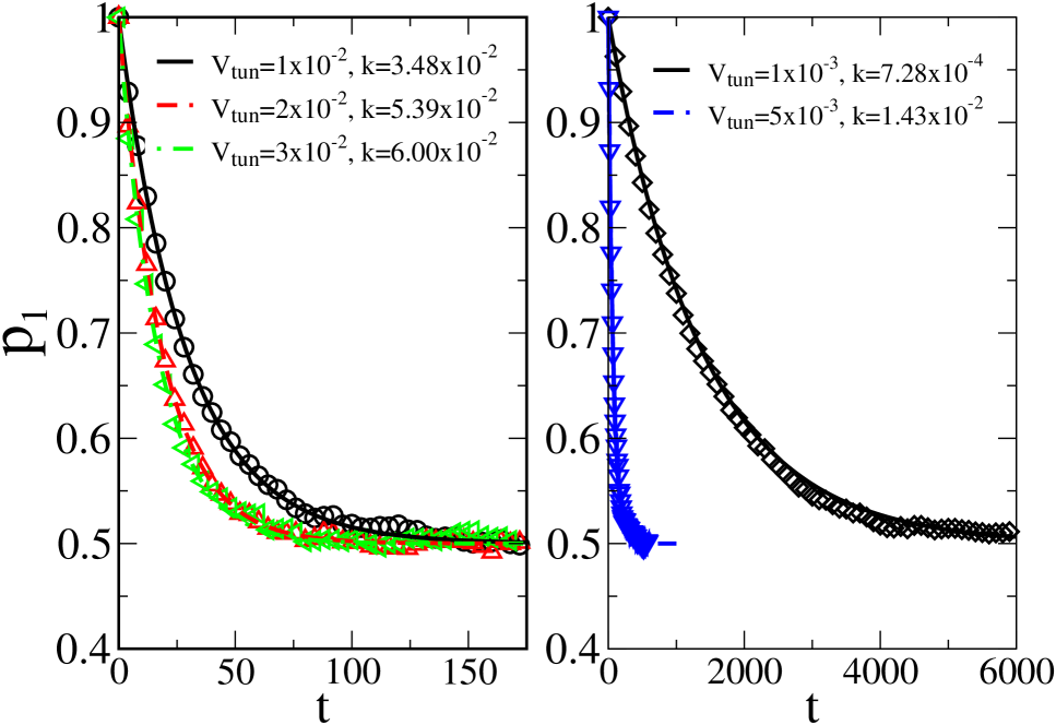
Figure 2: (Color online) Numerical relaxation of $p_{1}(t)$ (symbols) vs. the analytical results in Eqs. (7), (8), (10) (lines) for $\epsilon_{0}=0$, $\lambda=800$, $T=0.1$ and various values of $V_{\rm tun}$ shown in the plot numerics . For $V_{\rm tun}=0.001$, ET is nearly non-adiabatic, while for $V_{\rm tun}=0.03$ already close to adiabatic ET with $k^{(\rm ad)}=0.066$, from the ensemble perspective. The numerically fitted values of $k_{\rm num}$ (not shown) agree with the theoretical results shown in the plot with the accuracy better than 0.5% except for $V_{\rm tun}=0.001$ (about 4%). $N=10^{4}$ particles are used in simulations.

In this Letter we focus on the trajectory counterpart of this well-known ensemble theory. It can be obtained as follows. We propagate overdamped (with $M=0$) Langevin dynamics (4) on one potential surface. Once the threshold $x^{*}$ is reached the quantum hop on another surface occurs with the LZS probability (1), where $v=\delta x/\delta t$, $\delta t$ is the time integration step, and $\delta x$ is the $x$ displacement by crossing the threshold. After a quantum jump, Langevin dynamics is continuously propagated on the other surface, on so on. Notice that even if for $\delta t\to 0$ the formal limit of $\delta x/\delta t$ does not exist in a mean-square sense for the strictly overdamped dynamics, at any finite $\delta t$, $v$ is finite. The overdamped dynamics of the reaction coordinate leads, however, to an effective linearization of Eq. (1) in $f(v)$, $P_{\rm LZ}(v)\approx f(v)$, i.e. the results do not depend on whether we use Eq. (1), or (2) in simulations. This is our first remarkable result which is completely confirmed by numerics and agrees with the Zusman equations theory. We consider the symmetric case $\epsilon_{0}=0$ in this work. By propagating many particles simultaneously starting from the quantum state “1” and distributing initial $x(0)$ in accordance with $P^{(eq)}_{1}(x)$, we can keep track of the state populations. The corresponding results in Fig. 2 numerics agree remarkably well with the theoretical result in Eqs. (6)-(10). In other words, the ensemble averaged trajectory result nicely agrees with the analytical solution of Zusman equations. For a very small $V_{\rm tun}$, ET occurs non-adiabatically with the MLD rate. Upon increase of $V_{\rm tun}$, adiabatic transport regime is gradually approaching. It is almost reached for $V_{\rm tun}=0.03$ in Fig. 2.

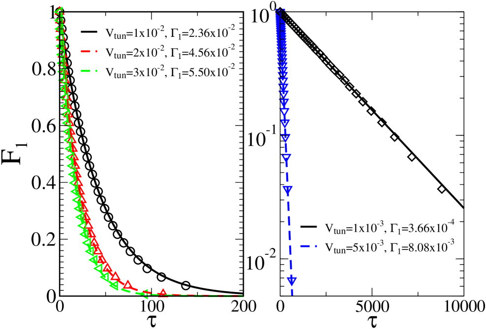
Figure 3: (Color online) Survival probability in one electronic state on the ensemble level. Parameters are the same as in Fig. 2. Numerical results are depicted by symbols, whereas an exponential decay with the rate in Eq. (11) is shown by lines.

Trajectory simulations contain, however, much more information than Zusman equations can deliver. We can study also the residence time distributions (RTDs) in the electronic states. The RTD distribution on the ensemble level can be obtained by preparing all the particles in one state, with the reaction coordinate initially thermally equilibrated and taking out particles once they jumped to another state until no particles remained in the initial state. The corresponding survival probability $F_{1}(\tau)$ decays single-exponentially, see in Fig. 3, however, with the rate $\Gamma_{1}$, which is different from the above $k_{1}$. Indeed, on theoretical grounds one can maintain that

$$\frac{1}{\Gamma_{1,2}}=\frac{1}{k_{1,2}^{\rm(nad)}}+\tau^{\rm(ad)}_{1,2},$$ (11)

i.e. the average time to make a transition is the sum of the average time to reach the threshold $x^{*}$ and of the inverse of the nonadiabatic tunneling rate. Indeed, numerics remarkably agree with this statement, see in Fig. 3. Furthermore, for a Markovian dynamics it must be $\Gamma_{1,2}=k_{1,2}$. This is indeed the case in the nonadiabatic ET regime characterized by MLD rate. However, dynamics of electronic transitions becomes increasingly non-Markovian upon taking adiabatic corrections into account with the increase of $V_{\rm tun}$. This is in spite of a single-exponential character of the ET kinetics on the ensemble level! Ref. GoychukJCP05 already pointed out on a similar very paradoxical situation: a highly non-Markovian bursting process can have a nearly exponentially decaying autocorrelation function. Indeed, a short inspection of a single trajectory realization of electronic transitions in such a non-Markovian regime depicted in Fig. 4 reveals immediately its non-Markovian character. Bursting provides a visual proof GoychukJCP05 . Notice that a popular statement that in adiabatic ET regime electrons just follow to nuclear transitions is in fact very misleading on the level of single electron trajectories. This is so because electron jumps only at the level crossings (in the contact approximation) and the ensemble description on the level of populations relaxation completely misses this very essential quantum mechanical feature. ET remains quantum even within this adiabatic seemingly fully classical regime! And namely this causes a quantum breaking of ergodicity discovered next.

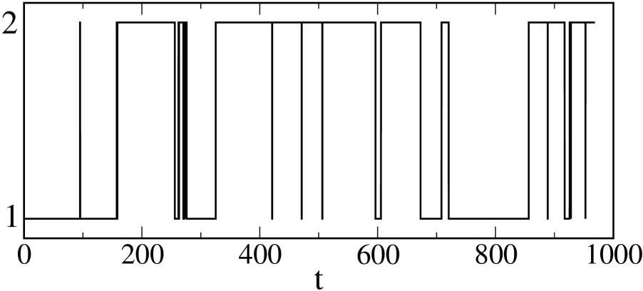
Figure 4: Quantum state trajectory realization in non-Markovian regime with broken ergodicity. $\epsilon_{0}=0$, $\lambda=800$, $T=0.1$, and $V_{\rm tun}=0.01$.

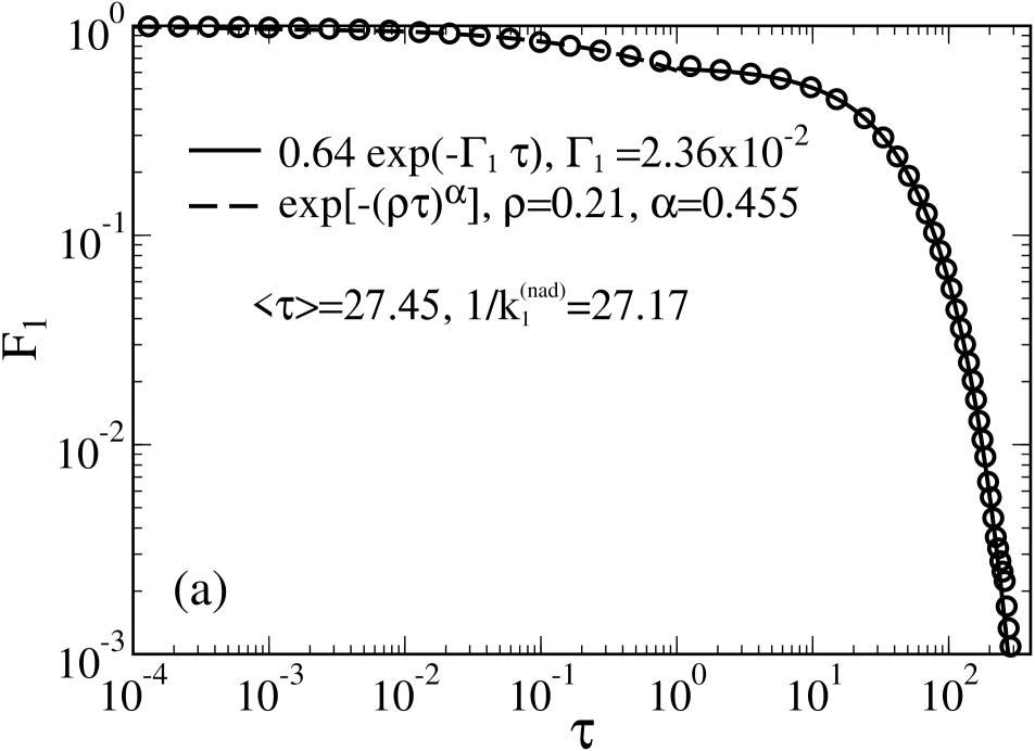
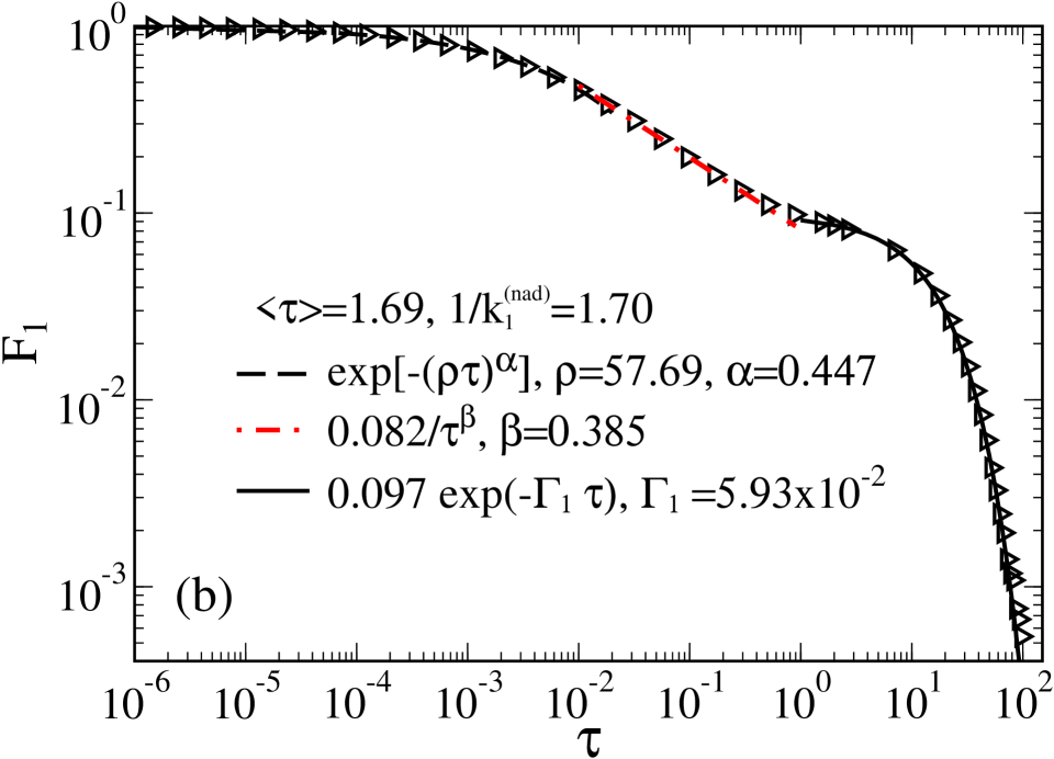
Figure 5: (Color online) Survival probability in one electronic state on a single trajectory level. Parameters are the same as in Fig. 2, and (a) $V_{\rm tun}=0.01$ (as in Fig. 4), (b) $V_{\rm tun}=0.04$. Numerical results are depicted by symbols and their fits by lines detailed in the plots.

Indeed, the study of survival probabilities based on single very long trajectories reveals a real surprise indicating breaking of ergodicity in this profoundly non-Markovian regime. The corresponding survival probability in a state is depicted in Fig. 5, (a). It is profoundly non-exponential, very differently from the corresponding ensemble result in Fig. 3. The rate $\Gamma_{1}$ describes only the tail of distribution, which is initially stretched exponential. It can possess also an intermediate power law regime for a larger $V_{\rm tun}$, see part (b) in Fig. 5, where the exponential tail has weight less than 10%. Very surprisingly, the mean residence time is well described by the inverse of the Marcus-Levich-Dogonadze rate, $\langle\tau_{i}\rangle=1/k_{i}^{\rm(nad)}$. This can be explained within a modification of the classical level-crossing theory Papoulis . Let us take formally into account small inertial effects (keeping first $M$ finite). Then, the process $v(t)$ is not singular. Consider dynamics in the state $i$. Assuming stationarity of $x(t)$, the averaged number of level crossings $n_{i}({\cal T})$ within a very long time interval ${\cal T}$ is Papoulis $n_{i}({\cal T})={\cal T}P_{i}^{(eq)}(x^{*})\langle|v(t)|\rangle_{x(t)=x^{*}}$, and hence $\langle\tau_{i}\rangle^{-1}=\lim_{{\cal T}\to\infty}n_{i}({\cal T})/{\cal T}=P_{i}^{(eq)}(x^{*})\langle|v(t)|\rangle_{x(t)=x^{*}}$. By the same token and taking into account the probability (1) to make a quantum jump to another state at each level crossing we obtain

$$\langle\tau_{i}\rangle^{-1}=P_{i}^{(eq)}(x^{*})\langle|v|P_{\rm LZ}(v)\rangle_{x(t)=x^{*}}\;\;.$$ (12)

Averaging in (12) with Maxwellian equilibrium $P_{M}(v)$ yields a very important result

$$\langle\tau_{i}\rangle^{-1}=k_{i}^{\rm(nad)}R(z=v_{0}/v_{T})\;,$$ (13)

where

$$R(z)=\sqrt{\frac{2}{\pi z^{2}}}-\frac{1}{2\pi}G^{\,3,0}_{0,3}\Bigg{\lparen}\begin{smallmatrix}-\\ \frac{1}{2},0,-\frac{1}{2}\end{smallmatrix}\Bigg{|}\,\frac{z^{2}}{8}\Bigg{\rparen}\quad$$ (14)

is a renormalization function taking inertial effects into account. It is expressed via a Meijer G-function Gradstein , and $v_{0}=\pi|V_{\rm tun}|^{2}x_{0}/(\hbar\lambda)$ is a characteristic tunnel velocity. Numerically, $R(z)\approx\exp(-1.57z^{0.9})$ for $0<z<0.1$ with the accuracy of about 10%. In the formal overdamped limit, $\lim_{M\to 0}R(v_{0}/v_{T})=1$, and we obtain $\langle\tau_{1}\rangle^{-1}=k_{1}^{\rm(nad)}$, in agreement with numerics. Moreover, we did also numerics which include inertial effects in Eq. (4) and confirm the analytical result in (13), (14) remark . The observed ergodicity breaking is thus not an artifact of the overdamped singular approximation. It expresses quantum nature of electron transfer even in adiabatic regime as manifested on the level of single molecule dynamics.

As a major result of this work, equations like Zusman equations and other quantum ensemble descriptions simply cannot be used to describe properties of profoundly non-Markovian single electron trajectories. This can be relevant e.g. for blinking quantum dots in non-exponential regimes, whenever the reaction coordinate dynamics is very essential TangMarcus . This is especially true for anomalously slow subdiffusive dynamics which is the subject of a separate follow-up work. The discovered ergodicity breaking in a simple and well-known model of charge transport dynamics is expected to influence a large body of current research.

Acknowledgment. Support of this research by the Deutsche Forschungsgemeinschaft (German Research Foundation), Grant GO 2052/1-2 is gratefully acknowledged.

References

- (1) F. D. Stefani, J. P. Hoogenboom, and E. Barkai, Phys. Today 62(2), 34 (2009); E. Barkai, Y. Garini, and R. Metzler, Phys. Today 65(8), 29 (2012).
- (2) R. Zwanzig, Proc. Natl. Acad. Sci. (USA) 85, 2029 (1988); H. Bässler, Phys. Rev. Lett. 58, 767(1987).
- (3) P. Hänggi, P. Talkner, and M. Borkovec, Rev. Mod. Phys. 62, 251 (1990).
- (4) I. Goychuk and V. O. Kharchenko, Phys. Rev. Lett. 113, 100601 (2014).
- (5) A. Nitzan, Chemical Dynamics in Condensed Phases: Relaxation, Transfer and Reactions in Condensed Molecular Systems (Oxford University Press, Oxford, 2006)
- (6) L. D. Landau, Phys. Z. Sowjetunion 2, 46(1932); C. Zener, Proc. R. Soc. London A 137, 696 (1932); E. C. G. Stueckelberg, Helv. Phys. Acta 5, 369 (1932).
- (7) L. D. Zusman, Chem. Phys. 49, 295 (1980); I. V. Alexandrov, Chem. Phys. 51, 449 (1980).
- (8) A. Garg, J. N. Onuchic, and V. Ambegaokar, J. Chem. Phys. 83, 4491 (1985).
- (9) L. Hartmann, I. Goychuk, and P. Hänggi, J. Chem. Phys. 113, 11159 (2000); J. Chem. Phys. 115, 3969 (2001).
- (10) J. Tang and R. A. Marcus, Phys. Rev. Lett. 95, 107401 (2005).
- (11) R. A. Marcus, J. Chem. Phys. 24, 966 (1956); 26, 867 (1957); Discuss. Faraday Soc. 29, 21 (1960).
- (12) V. G. Levich and R. R. Dogonadze, Dokl. Akad. Nauk SSSR 124, 123 (1959) (in Russian) [Proc. Acad. Sci. Phys. Chem. Sect. 124, 9 (1959)].
- (13) I. S. Gradstein and I. M. Ryzhik, Table of Integrals, Series, and Products (Academic, New York, 1965).
- (14) Time is scaled in units of , in units of , and other energy parameters in units of . For a typical ps, (in spectroscopic units), and corresponds to , whereas to or room temperatures.
- (15) I. Goychuk, J. Chem. Phys. 112, 164506 (2005).
- (16) A. Papoulis, Probability, Random Variables, and Stochastic Processes, 3d ed. (McGraw-Hill Book Company, New York, 1991), Ch. 16.
- (17) A detailed treatment will be presented elsewhere.