Mutual Radiation Impedance of
Uncollapsed CMUT Cells with Different Radii

Abstract

A polynomial approximation is proposed for the mutual acoustic impedance between uncollapsed capacitive micromachined ultrasonic transducer (CMUT) cells with different radii in an infinite rigid baffle. The resulting approximation is employed in simulating CMUTs with a circuit model. A very good agreement is obtained with the corresponding finite element simulation (FEM) result.

I Introduction

An array of transducers is usually employed for generating powerful and focused ultrasonic beams for imaging or therapy purposes [1]. Mutual interactions between the cells of the array are especially important when the mechanical impedance of cells is relatively low. This is exactly the case for capacitive micromachined transducers (CMUT) which provide a wide band operation in liquid immersion because of its low mechanical impedance [2]. Mechanics of uncollapsed CMUT cells can be accurately modelled with flexural disks with clamped edges [3]. It was shown that [4, 5] it is possible to accurately model an array of CMUT cells using an electrical circuit model coupled to a impedance matrix composed of self and mutual radiation impedances. Self and mutual radiation impedances of equal size CMUT cells in uncollapsed [6] and collapsed [7] mode can found in the literature.

Porter [8] was the first to quantify the mutual impedance between two identical flexural disks for different edge conditions and obtained an infinite series solution. Chan [9] extended this work to cover the mutual impedance of flexural disks with different radii. In both cases, the mutual impedance turns out to be an oscillatory and slowly decaying function of the distance between the two radiators. This implies that the acoustic coupling between all cells must be taken into account to accurately predict the performance of an array. This demanding requirement increases the computation time substantially. Therefore, a sufficiently accurate but computationally low-cost approximation is highly desirable to expedite the simulations of mutual interactions.

An approximation for the radiation impedance of the uncollapsed CMUT cells of equal size was presented earlier [5]. This approximation is extended to that of unequal size cells. It is verified in Section III performing a finite element method (FEM) simulation for a particular case.

II A Polynomial Approximation

In Chan’s work [9], the mutual impedance between two flexural disks of clamped edges with radii $a_{1}$ and $a_{2}$ and center-to-center separation of $d$ is found as

$$\begin{split}\frac{Z_{12}(ka_{1},ka_{2},kd)}{{\rho}c{\pi}{a_{1}}{a_{2}}}=3^{2}2^{7}\Bigg{\{}\frac{1}{(ka_{1})^{2}(ka_{2})^{2}}\\ \times\sum\limits_{m=0}^{\infty}\sum\limits_{n=0}^{\infty}\frac{\Gamma(m+n+1/2)}{m!n!\sqrt{2kd}}\Bigg{(}\frac{{a_{1}}^{m}{a_{2}}^{n}}{{d}^{m+n}}\Bigg{)}J_{3+m}(ka_{1})J_{3+n}(ka_{2})\\ \times[J_{m+n+\frac{1}{2}}(kd)+i(-1)^{m+n}J_{-m-n-\frac{1}{2}}(kd)]\Bigg{\}}\end{split}$$ (1)

where the reference is rms velocity, $\rho$ is the density of the medium, $c$ is the speed of sound and $k$ is the wavenumber.

For identical disks ($a_{1}=a_{2}=a$), an approximation for the mutual radiation impedance is given as [5]

$$\frac{Z_{12}(ka,kd)}{{\rho}c\pi a^{2}}~{}{\approx}~{}A(ka)\frac{\sin(kd)+j\cos(kd)}{kd}\,\,\,\,\mbox{for}\,\,\,\,ka<5.5$$ (2)

and $A(x)$ can be approximated with a $10^{th}$ order polynomial:

$$A(x)\approx\sum\limits_{n=0}^{10}p_{n}{x}^{n}$$ (3)

The values of $p_{n}$’s are tabulated in Table I.

Coefficient	Real Part	Imaginary Part
$p_{10}$	$-1.74841\cdot 10^{-7}$	$-2.07413\cdot 10^{-7}$
$p_{9}$	$-3.63059\cdot 10^{-7}$	$~{}~{}~{}6.41730\cdot 10^{-6}$
$p_{8}$	$~{}~{}~{}1.00277\cdot 10^{-4}$	$-7.76934\cdot 10^{-5}$
$p_{7}$	$-1.45594\cdot 10^{-3}$	$~{}~{}~{}4.43450\cdot 10^{-4}$
$p_{6}$	$~{}~{}~{}8.20869\cdot 10^{-3}$	$-1.06884\cdot 10^{-3}$
$p_{5}$	$-1.52895\cdot 10^{-2}$	$~{}~{}~{}5.31086\cdot 10^{-4}$
$p_{4}$	$-1.28941\cdot 10^{-2}$	$-2.40879\cdot 10^{-3}$
$p_{3}$	$-2.10234\cdot 10^{-2}$	$~{}~{}~{}1.44157\cdot 10^{-2}$
$p_{2}$	$~{}~{}~{}2.92992\cdot 10^{-1}$	$-7.06028\cdot 10^{-4}$
$p_{1}$	$-2.38707\cdot 10^{-3}$	$~{}~{}~{}1.36767\cdot 10^{-4}$
$p_{0}$	$~{}~{}~{}1.73311\cdot 10^{-4}$	$-8.68895\cdot 10^{-6}$

TABLE I: Coefficients of the approximate polynomial for $A(x)$

When the disks have different radii, finding an approximation is harder due to the cross-coupled $ka_{1}$ and $ka_{2}$ related terms in the mutual impedance expression. It can be numerically shown that the mutual impedance can be written very accurately as a summation of a separable component in $ka_{1}$ and $ka_{2}$, and an inseparable one as follows:

$$\frac{Z_{12}(ka_{1},ka_{2},kd)}{{\rho}c\pi a_{1}a_{2}}~{}{\approx}~{}B(ka_{1},ka_{2})\frac{\sin(kd)+j\cos(kd)}{kd}$$ (4)

where

$$B(ka_{1},ka_{2})=S(ka_{1})S(ka_{2})+jI(ka_{1},ka_{2})$$ (5)

where $S(x)$ is a complex-valued function with

$$S^{2}(x)=A(x)$$ (6)

With $S_{r}(x)$ and $S_{i}(x)$ real-valued functions, we write

$$S(x)=S_{r}(x)+jS_{i}(x)$$ (7)

From (6) and (7), $S_{r}(x)$ and $S_{i}(x)$ are found as

$$S_{r}(x)=\frac{1}{\sqrt{2}}\Bigg{(}A_{r}(x)+\sqrt{A_{r}(x)^{2}+A_{i}(x)^{2}}\Bigg{)}^{1/2}$$ (8)

$$S_{i}(x)=\frac{A_{i}(x)}{\sqrt{2}(A_{r}(x)+\sqrt{A_{r}(x)^{2}+A_{i}(x)^{2}})^{1/2}}$$ (9)

where $A_{r}(x)$ and $A_{i}(x)$ represent the real and imaginary parts of $A(x)$, respectively.

The inseparable component in (5), $I(x_{1},x_{2})$, is approximated as a polynomial in the following form

$$I(x_{1},x_{2})\approx(x_{1}-x_{2})^{2}\sum\limits_{m=0}^{5}\sum\limits_{n=0}^{5-m}q_{mn}{x_{1}}^{m}{x_{2}}^{n}$$ (10)

where the values of $q_{mn}$’s are given in Table II. We note that for $ka_{1}=ka_{2}=ka$, (4) reduces to (2).

Figs. 1 and 2 are the plots of real and imaginary parts of $B(ka_{1},ka_{2})$ as a function of $ka_{2}$ for various values of $ka_{1}$. The analytical solution and the approximate expression agree very well.

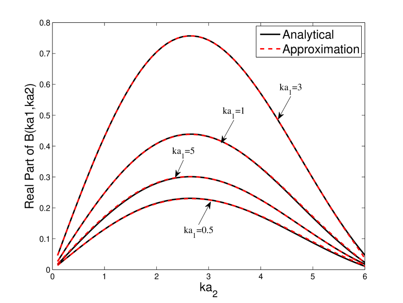
Figure 1: A comparison of the real parts of the analytical and approximate expressions for different values of $ka_{1}$ and $ka_{2}$.

Figure 2: A comparison of the imaginary parts of the analytical and approximate expressions for different values of $ka_{1}$ and $ka_{2}$.

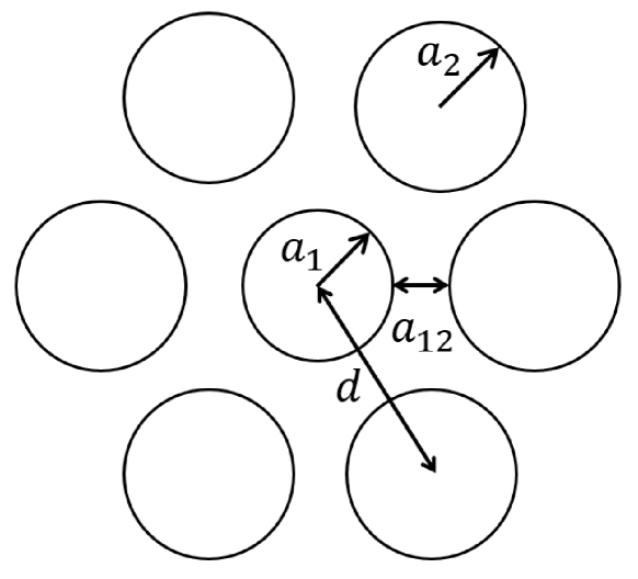
Figure 3: The geometry of CMUT element used for verification.

Coefficient	Value	Coefficient	Value
$q_{00}$	$-1.733\cdot 10^{-3}$	$q_{11}$	$-8.465\cdot 10^{-5}$
$q_{01},q_{10}$	$~{}~{}~{}4.502\cdot 10^{-3}$	$q_{12},q_{21}$	$~{}~{}~{}3.673\cdot 10^{-4}$
$q_{02},q_{20}$	$-3.003\cdot 10^{-3}$	$q_{13},q_{31}$	$-1.475\cdot 10^{-4}$
$q_{03},q_{30}$	$~{}~{}~{}8.407\cdot 10^{-4}$	$q_{14},q_{41}$	$~{}~{}~{}1.146\cdot 10^{-5}$
$q_{04},q_{40}$	$-1.091\cdot 10^{-4}$	$q_{22}$	$~{}~{}~{}1.298\cdot 10^{-5}$
$q_{05},q_{50}$	$~{}~{}~{}5.522\cdot 10^{-6}$	$q_{23},q_{32}$	$~{}~{}~{}2.596\cdot 10^{-6}$

TABLE II: Coefficients of the approximate polynomial for $I(x_{1},x_{2})$

III A Comparison of the Approximation with FEM

The accuracy and efficiency of the presented approximation is checked by employing it to couple CMUT cells in a cluster. We used (5) to model the mutual impedance between the central cell and peripheral cells of the 7-cell cluster depicted in Fig. 3 and we simulated this structure with an electrical circuit simulator capable of accepting frequency domain data. A transient analysis is performed using the equivalent circuit of CMUT cell [5]. Table III shows the geometric dimensions and parameters used. Equivalent circuit model simulation results are compared with FEM analysis results in Figs. 4 and 5, where a very good agreement is observed. Notice the amplitude and phase differences of center cell and edge cells. For example, at 2.99MHz the center CMUT cell does not move at all, while the maximum displacements of the edge cells and center cell occur at 3.39MHz and 4.90MHz, respectively. At 3.75MHz, the center cell and edge cells displacement magnitudes are equal with a 114^∘ phase difference.

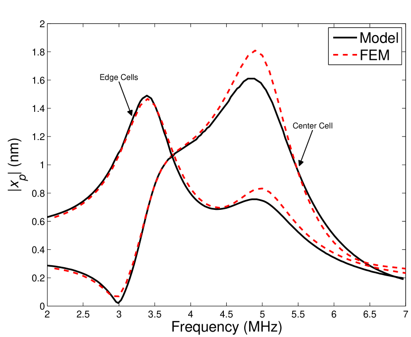
Figure 4: The magnitude of the peak displacement for the center and edge cells for an excitation voltage of 1V peak.

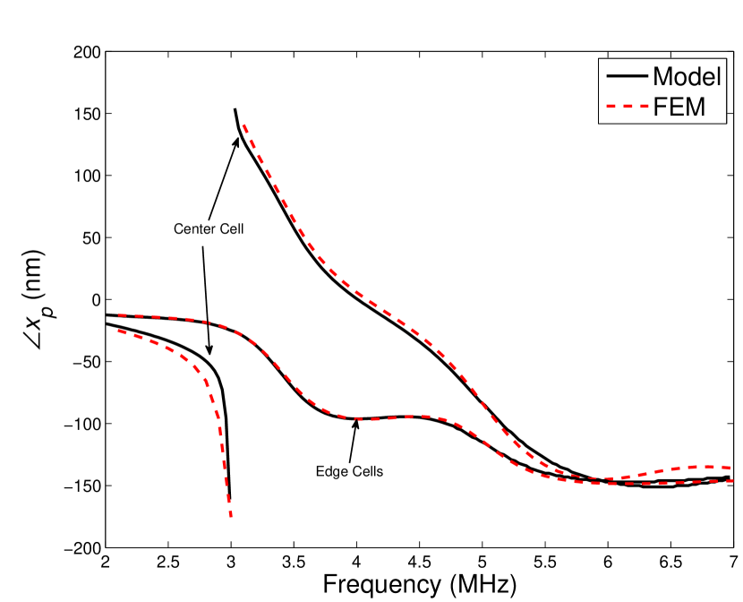
Figure 5: The phase of the peak displacement for the center and edge cells.

Parameter	Value
Center Cell Radius, $a_{1}$	$90~{}{\mu}$m
Edge Cell Radius, $a_{2}$	$104~{}{\mu}$m
Center-to-Edge-Cell Gap, $a_{12}$	$24.4~{}{\mu}$m
Gap Height, $t_{ga}$	$150~{}n$m
Membrane Thickness, $t_{m}$	$13~{}{\mu}$m
Insulator Thickness, $t_{i}$	$100~{}n$m
Young’s Modulus, $Y_{0}$	$320~{}$GPa
Density, $\rho$	$3270~{}$kg/m3
Poisson Ratio, $\sigma$	$0.263$
Bias Voltage, $V_{DC}$	$45~{}$V
Excitation, $V_{AC}$	$1$V peak

TABLE III: Parameters of the CMUT cells used in simulation

IV Conclusions

A mutual impedance approximation is presented for clamped flexural disks having different radii. The resulting approximation is inserted into the electrical equivalent circuit to couple CMUT cells in a cluster and a very good agreement with the FEM results is obtained. This approximation makes it possible to design mixed-sized CMUT arrays using circuit simulation tools.

References

- [1] F. Y. Yamaner, S. Olcum, H. K. Oguz, A. Bozkurt, H. Koymen, and A. Atalar, “High-power CMUTs:design and experimental verification,” IEEE Trans. Ultrason., Ferroelect., Freq. Contr., vol. 59, pp. 1276–1284, 2012.
- [2] K. K. Park, M. Kupnik, H. J. Lee, B. T. Khuri-Yakub, and I. O. Wygant, “Modeling and measuring the effects of mutual impedance on multi-cell CMUT configurations,” in Proc. IEEE Ultrason Symp., 2010, pp. 431 –434.
- [3] I. Ladabaum, X. Jin, H. T. Soh, A. Atalar, and B. T. Khuri-Yakub, “Surface micromachined capacitive ultrasonic transducers,” IEEE Trans. Ultrason., Ferroelect., Freq. Contr., vol. 45, pp. 678–690, 1998.
- [4] H. Köymen, A. Atalar, E. Aydogdu, C. Kocabas, H. Oguz, S. Olcum, A. Ozgurluk, and A. Unlugedik, “An improved lumped element nonlinear circuit model for a circular CMUT cell,” IEEE Trans. Ultrason., Ferroelect., Freq. Contr., vol. 59, pp. 1791–1799, 2012.
- [5] H. Oğuz, H. Köymen, and A. Atalar, “Equivalent circuit-based analysis of cMUT cell dynamics in arrays,” IEEE Trans. Ultrason., Ferroelect., Freq. Contr., vol. ??, pp. ????–????, 2013.
- [6] M. N. Senlik, S. Olcum, H. Köymen, and A. Atalar, “Radiation impedance of an array of circular capacitive micromachined ultrasonic transducers,” IEEE Trans. Ultrason., Ferroelect., Freq. Contr., vol. 57, pp. 969–976, 2010.
- [7] A. Ozgurluk, A. Atalar, H. Koymen, and S. Olcum, “Radiation impedance of collapsed capacitive micromachined ultrasonic transducers,” IEEE Trans. Ultrason., Ferroelect., Freq. Contr., vol. 59, pp. 1301–1308, 2012.
- [8] D. T. Porter, “Self-and mutual-radiation impedance and beam patterns for flexural disks in a rigid plane,” J. Acoust. Soc. Am., vol. 36, pp. 1154–1161, 1964.
- [9] K. C. Chan, “Mutual acoustic impedance between flexible disks of different sizes in an infinite rigid plane,” J. Acoust. Soc. Am., vol. 42, pp. 1060–1063, 1967.