Abstract

We present a method for modelling the covariance structure of tensor-variate data, with the ulterior aim of learning an unknown model parameter vector using such data. We express the high-dimensional observable as a function of this sought model parameter vector, and attempt to learn such a high-dimensional function given training data, by modelling it as a realisation from a tensor-variate Gaussian Process (GP). The likelihood of the unknowns given training data, is then tensor-normal. We choose vague priors on the unknown GP parameters (mean tensor and covariance matrices) and write the posterior probability density of these unknowns given the data. We perform posterior sampling using Random-Walk Metropolis-Hastings. Thereafter we learn the aforementioned unknown model parameter vector by performing posterior sampling in two different ways, given test and training data, using MCMC, to generate 95$\%$ HPD credible region on each unknown. We make an application of this method to the learning of the location of the Sun in the Milky Way disk.

1 Introduction

A cornerstone of scientific pursuit involves seeking the value of an unknown model parameter, given data that constitutes measurements of an observable. Such an exercise is of course relevant only when the observable is a function of the model parameter. Knowing the functional relationship between this observable and the model parameter, one can then inversely learn the value of the model parameter at which the data at hand is realised (Ramsay and Silverman, 2014; Hofmann, 2011; Tarantola, 2005). The Bayesian equivalent of this approach constitutes sampling from the posterior predictive density of the unknown parameter, given the data and the model for the aforementioned functional relationship. However, this very functional relationship (between the observable and the unknown parameter), may not be known apriori. The standard approach within supervised learning, is to then train the model for this function using training data (Gelman et al., 1995; Neal, 1998), in order to subsequently predict the unknown parameter, given the data at hand. If the observable is high-dimensional (tensor-valued in general), this function is rendered high-dimensional (tensor-variate) as well, leading us to the inverse learning of the unknown model parameter in a high-dimensional situation (Alquier et al., 2011). Conventional inverse problem approaches are typically in low-dimensions (Cavalier, 2008; Tarantola, 2005). However, as the procurement of high-dimensional data becomes more common in different scientific disciplines (Zhao et al., 2014; Xu et al., 2012), we will more commonly encounter the difficult task of inversely learning a model parameter vector, subsequent to the supervised learning of a high-dimensional function.

We present a new method to perform Bayesian inverse learning on an unknown model parameter vector, given test and training data. The core of our methodology lies in the nonparametric supervised learning of the tensor-variate function of the model parameter vector that gives the observable, using tensor-variate training data. We achieve this by modelling such a function by treating it as sampled from a Gaussian Process of corresponding dimensionality, i.e. a tensor-variate Gaussian Process, the mean and covariance structure of which we learn. Such modelling would in turn imply that the joint probability of a set of realisations of this function, (which equivalently is a set of values of the observable), is the tensor-normal density.

Earlier Hoff, P. D. (2011) used Tucker decomposition to extract the covariance matrices of a tensor-variate Gaussian Process (GP) and proceeded to compute a maximum likelihood solution for the covariance matrices and the mean tensor of the GP. Zhao et al. (2014) introduced tensor kernels in order to compute the distance between two tensors for which (tensor) kernel parametrisation has been undertaken. Subsequently, they applied this to a graph classification problem. Hou et al. (2015) solved a tensor-variate Gaussian Process-based regression problem using a local least square method–they focus on the complexity of tensor GP regression for large data sets.

However, in our work the aim is to learn an unknown model parameter vector; this is accomplished via the supervised learning of the functional relationship between itself and the tensor-shaped data, where the said function is modelled using a tensor-variate GP. Both the supervised learning of this function, as well as the inverse learning of the unknown model parameter vector, are undertaken in a Bayesian framework, using MCMC-based inference (Random-Walk Metropolis-Hastings or RW; see Robert and Casella (2004)). To this effect, we do indeed learn the covariance structure of the tensor-variate GP, though our aim takes us beyond this exercise. In fact, we propose three different ways of learning the multiple covariance matrices of the GP, depending on availability of information and feasibility constraints (which are motivated by the dimensions of such matrices). Furthermore, we undertake the learning of the sought model parameter vector by performing RW-based sampling from the posterior predictive density of the unknowns, given the test+training data and the learnt model of the GP (covariance and mean structure), as well as by performing such sampling from the joint posterior probability density of the model parameter and the GP parameters, given all data.

We implement this methodology to learn the location vector of the Sun in the disk of the Milky Way galaxy. The basis of this ambition lies in the fact that Galactic features affect stellar velocities, so that in principle, an observed set of stellar velocity vectors can be treated to be a function of the vector of the Galactic feature parameters (see Chakrabarty et al. (2015)). However, the feature parameters of interest are related to the galactocentric solar location in known ways. Thus, equivalently, the observed set of stellar velocity vectors can be treated to be a function of the solar location vector. Here the set of velocity vectors–i.e. the matrix of stellar velocity components–is that of a chosen number of stellar neighbours of the Sun. It is only after learning the said function, that we can predict the unknown solar location, given the data. Here, training data comprises matrices, each row of which is the velocity vector of a stellar neighbour of the Sun, with each such matrix generated at a fiduciary solar location (design point), in astronomical simulations. Thus the training data is 3-tensor (set of matrices, with each generated at a design point). The test data is available as a matrix of velocity measurements of stellar neighbours of the Sun (Chakrabarty, 2007). We learn the aforementioned function by modelling it with a high-dimensional Gaussian Process, the parameters of which we learn using MCMC techniques. Thereafter, we perform inverse Bayesian learning of the unknown solar location vector.

2 Method

Let the observable $\boldsymbol{V}$ be a $k-1$-rank tensor, i.e. $\boldsymbol{V}\in{\mathbb{R}}^{m_{1}\times m_{2}\ldots\times m_{k-1}}$, $m_{j}$ is a positive integer, $j=1,\ldots,k-1$. We treat $\boldsymbol{V}$ to be an unknown function of the model parameter $\boldsymbol{S}$, where $\boldsymbol{S}\in{\mathbb{R}}^{d}$. Thus, we define $\boldsymbol{V}=\boldsymbol{\xi}(\boldsymbol{S})$, where $\boldsymbol{\xi}(\cdot)$ is this unknown function, where–by virtue of this equation–$\boldsymbol{\xi}(\cdot)$ is a $k-1$-tensor-variate function itself. We are going to predict the value $\boldsymbol{s}^{(test)}$ of $\boldsymbol{S}$ at the new or test data ${\bf v}^{(test)}$. In order to do this, the unknown tensor-variate function $\boldsymbol{\xi}(\cdot)$ needs to be learnt, given the training data ${\bf D}:=\{(\boldsymbol{s}_{1}^{(*)},\boldsymbol{v}_{1}),\ldots,(\boldsymbol{s}_{n}^{(*)},\boldsymbol{v}_{n})\}$, where $\boldsymbol{s}_{i}^{(*)}$ is the $i$-th design point at which the value $\boldsymbol{v}_{i}$ of the observable is generated, $i=1,\ldots,n$. Such supervised learning can be done using parametric regression techniques, (such as fitting with splines/wavelets). In the conventional inverse problem approach, the $\boldsymbol{\xi}(\cdot)$ learnt using such techniques, will thereafter need to be inverted and this inverse operated upon the test data, to yield the value $\boldsymbol{s}^{(test)}$ of $\boldsymbol{S}$ at which the test data is realised. The shortcoming of using the method of splines/wavelets is that the correlations between the components of the high-dimensional function $\boldsymbol{\xi}(\cdot)$ are not properly learnt. Moreover, such parametric regression causes computational difficulties as the dimensionality of the observable increases.

This drives us to use Gaussian Process (GP) based methods–we treat the $k-1$-tensor-variate function as a realisation from a $k-1$-tensor-variate GP. Upon learning the parameters of this GP using the training data, we are then able to write the posterior predictive of $\boldsymbol{S}$ given the test+training data and the GP parameters. This is the standard supervised learning scheme that we are going to use here, except, in one case we sample from the posterior predictive of $\boldsymbol{s}^{(test)}$ given all data, and alternatively, perform posterior sampling from the joint posterior probability density of all unknowns, given all data (test and training). In each case, we extract the marginal posterior of each parameter given the data, using our MCMC-based inference scheme (see Section 3 of supplementary material).

We treat $\boldsymbol{\xi}(\cdot)$ as a realisation from a tensor-variate GP, where the rank of this tensor-variate process is $k-1$. It then follows that the observable $\boldsymbol{V}$ is also a realisation from this GP. As a result, the set of $n$ realisations of this observable, i.e. the training data ${\boldsymbol{D}}=\{\boldsymbol{v}_{1},\ldots,\boldsymbol{v}_{n}\}$, follows a $k$-variate tensor normal distribution with mean tensor $\boldsymbol{M}$ and $k$ covariance matrices $\boldsymbol{\Sigma}_{1},...,\boldsymbol{\Sigma}_{k}$ : $\{\boldsymbol{v}_{1},\ldots,\boldsymbol{v}_{n}\}\sim{\cal TN}_{k}(\boldsymbol{M},\boldsymbol{\Sigma}_{1},...,\boldsymbol{\Sigma}_{k})$, so that the likelihood of mean tensor $\boldsymbol{M}$, and the covariance matrices $\boldsymbol{\Sigma}_{1},...,\boldsymbol{\Sigma}_{k}$, given the training data, is a tensor-normal density:

$$p(\boldsymbol{D}|\boldsymbol{M},\boldsymbol{\Sigma}_{1},...,\boldsymbol{\Sigma}_{k})\propto$$ (1)

$$\exp(-\|(\boldsymbol{V}-\boldsymbol{M})\times_{1}\boldsymbol{A}_{1}^{-1}...\times_{k}\boldsymbol{A}_{k}^{-1}\|^{2}/2)$$

where the covariance matrix $\boldsymbol{\Sigma}_{p}=\boldsymbol{A}_{p}\boldsymbol{A}^{T}_{p}$, $p=1,...,k$, i.e. $\boldsymbol{A}_{p}$ is the unique square-root of the positive semi-definite covariance matrix $\boldsymbol{\Sigma}_{p}$. The operator “$\times_{p}$” represents the $p$-mode multiplication of a tensor with a matrix. The tensor-normal distribution is extensively discussed in the literature, (Xu et al., 2012; Hoff, P. D., 2011).

2.1 Different ways of learning the covariance matrices

If we were to propose to learn each element of each covariance matrix using MCMC (or at least the upper triangle of each such matrix, invoking symmetry of covariance matrices), we would be committing to the learning of a very large number of parameters indeed. The computational complexity increases rapidly when the number of observations increases. In order to reduce the task to be computationally tractable, one possibility is to use kernel parametrisation of the covariance matrices $\boldsymbol{\Sigma}_{1},...,\boldsymbol{\Sigma}_{k}$, and then learn the parameters of these kernels using MCMC.

Of the $i$-th covariance matrix, let the $jp$-th element be $\sigma_{jp}^{(i)}$. Then $\sigma_{jp}^{(i)}$ bears information about the covariance amongst the slices of the data set achieved at the $j$-th and $p$-th input variables. The “input variable” referred to here, is the variable in the input space, i.e. the model parameter $\boldsymbol{S}$. We define $\sigma_{jp}^{(i)}=K_{i}(\boldsymbol{s}_{j},\boldsymbol{s}_{p})$, where $K_{i}(\boldsymbol{s}_{j},\boldsymbol{s}_{p})$ is the kernel function $K_{i}(\cdot,\cdot)$, computed at the $j$-th and $p$-th input variables. Thus, the number of unknown parameters involved in the learning of the covariance function of the high-dimensional GP would then reduce to the number of hyper-parameters of the kernel function $K_{i}(\cdot,\cdot)$, $i=1,\ldots,k$. In other words, such kernel parametrisation does help reduce the number of unknowns that need to be inferred upon, using MCMC.

However, there are two situations in which we might opt out of practising kernel parametrisation. Firstly, such parametrisation may cause information loss that may not be acceptable; one may then resort to learning each element of the covariance matrix (Aston and Kirch, 2012). Another situation when we avoid kernel parametrisation is the following. Let us consider the $i$-th covariance matrix that holds information about the covariance amongst slices of the training data achieved at distinct indices for $i$, i.e. along the $i$-th direction. We may not always be aware of the variable in the input space that takes different values at the different $i$-indices. In such situations, kernel parametrisation of elements of the covariance matrix is not possible, since such kernels need to be computed at pairwise different values of the input variable.

In such situations, we would opt to learn the elements of the covariance matrix directly using MCMC. However, as discussed above, such can be computationally daunting. If the computational task is then rendered too time intensive, then we will perform an empirical estimation of the $i$-th covariance matrix. An empirical estimate can be performed by collapsing each high-dimensional data slice along all-but-one directions (other than the $i$-th direction), to achieve a vector in place of the original high-dimensional slice at the $i$-th index value. The vectors at the different $i$-indices then possess the compressed information from all the relevant dimensions of the data variable. The covariance matrix $\boldsymbol{\Sigma}_{i}$ is then approximated by an empirical estimate of the covariance amongst such vectors.

Indeed such an empirical estimate of any covariance matrix may then be easily generated, but it indulges in linearisation amongst the different dimensionalities of the observable. So when the $\boldsymbol{\Sigma}_{i}$ covariance matrix bears information about high-dimensional slices of the data at the different $i$-indices, such linearisation may cause loss of information about the covariance structure.

In summary, we model the covariance matrices as kernel parametrised or empirically-estimated or learnt directly using MCMC. A computational worry is the burden of inverting any of the covariance matrices; for a covariance matrix that is $m_{i}\times m_{i}$, the computational order for matrix inversion is well known to be $O(m^{3}_{i})$ (Knuth, 1997).

In our application, when we implement kernel parametrisation, we choose to use the Squared Exponential (SQE) covariance kernel. However, other kinds of kernel functions can be used. In the application discussed in this paper, the data is continuous and we assume the covariance structure to be stationary. It is recalled that the SQE form can be expressed as

$$K(\boldsymbol{s}_{j},\boldsymbol{s}_{p})={a_{jp}\exp\left(-(\boldsymbol{s}_{j}-\boldsymbol{s}_{p})^{T}\boldsymbol{Q}(\boldsymbol{s}_{j}-\boldsymbol{s}_{p})\right)}$$ (2)

where $\boldsymbol{s}_{j}$ is the $j$-th value of the input vector and $\boldsymbol{Q}$ is a diagonal matrix, an element of which is the reciprocal of a correlation length scale. These correlation length scales are then unknown parameters that are learnt from the data using MCMC. As we see from Equation 2, for $\boldsymbol{S}\in{\mathbb{R}}^{d}$, $\boldsymbol{Q}$ is a $d\times d$-dimensional square diagonal matrix, so that there are $d$ unknown correlation lengths to learn using MCMC for a given covariance matrix. Here $a_{jp}$ is the amplitude of the covariance. However, we set $\left[a_{jp}\exp\left(-(\boldsymbol{s}_{j}-\boldsymbol{s}_{p})^{T}\boldsymbol{Q}(\boldsymbol{s}_{j}-\boldsymbol{s}_{p})\right)\right]\equiv A\left[\exp\left(-(\boldsymbol{s}_{j}-\boldsymbol{s}_{p})^{T}\boldsymbol{Q}^{\prime}(\boldsymbol{s}_{j}-\boldsymbol{s}_{p})\right)\right]$, where $A$ is a global scale such that all local amplitudes are $<1$ and the $\boldsymbol{Q}^{\prime}$ diagonal matrix contains the reciprocal of the correlation length scales, modulated by such local amplitudes. The global scale $A$ is subsumed as the scale to one of the covariance matrices of the tensor-normal distribution at hand–this is the matrix, the elements of (the upper/lower triangle of) which are learnt directly using MCMC, i.e. without resorting to any parametrisation or to any form of empirical estimation.

We write the likelihood using Equation 1. Using this likelihood and adequately chosen priors on the unknown parameters, we can write the posterior density of the unknown parameters given the training data, where the unknowns include parameters of the covariance matrices–if kernel parametrised, or elements of such a matrix itself–if being directly learnt using MCMC. Once this is achieved, we use the RW MCMC technique to sample from the joint posterior probability density of the unknown parameters of each covariance matrix and mean tensor, given the training data. We generate the marginal posterior probability densities of each unknown parameter given training data, and identify the 95$\%$ Highest Probability Density (HPD) credible regions on each parameter.

Thereafter, the prediction of $\boldsymbol{s}^{(test)}$ can be performed.

We treat the tensor variate normal distribution as the sum of a mean function and a zero mean normal distribution. The mean tensor is $\boldsymbol{M}\in R^{m_{1}\times m_{2}...\times m_{k}}$. We work in this application by removing an estimate of the mean tensor from the non-zero mean tensor-normal distribution. In this application, we have used the maximum likelihood estimation of the mean tensor.

3 Application

We are going to illustrate our method using an application on astronomical data. Following on from the introductory section, in this application the set of measurements that are invoked to allow for the learning of the location of the Sun in the Milky Way (MW) disk (assumed a two-dimensional object), happens to be the velocities of the stars that surround the Sun, as measured by the observer, i.e. us, seated at the Sun, since on galactic scales, our location on the MW disk is equivalent to the solar location. A sample of our neighbouring stars had their velocity vectors measured by the Hipparcos satellite (see Chakrabarty (2007) for details). Thus, this measured or test data is a matrix, each row of which is a star’s velocity vector.

If a sample of stars are allowed to evolve under the influence of certain Galactic features, from a primordial time to the current, these features will drive stars of different velocities to different locations on the MW disk. Thus, the stars that end up in the neighbourhood of the Sun, have velocity vectors as given by the test data matrix, because of the influence of the Galactic features on them. Thus, the matrix of velocities of stars in the solar neighbourhood is related to the parameters of these Galactic features. Since such feature parameters can be scaled to the galactocentric location vector of the Sun, (discussed below in Section 4.2), we treat the matrix of stellar velocities $\boldsymbol{V}$ to be functionally related to the solar or observer location vector $\boldsymbol{S}$, i.e. $\boldsymbol{V}=\boldsymbol{\xi}(\boldsymbol{S})$. Here for $\boldsymbol{V}\in{\mathbb{R}}^{m_{1}\times m_{2}\times n}$ and $\boldsymbol{S}\in{\mathbb{R}}^{d}$, $\boldsymbol{\xi}:{\mathbb{R}}^{d}\longrightarrow{\mathbb{R}}^{m_{1}\times m_{2}\times n}$.

We learn this function $\boldsymbol{\xi}(\cdot)$ using training data that comprises $n$ pairs of values of chosen solar location vector and the stellar velocity matrix generated at this solar location. Thus, the full training data is a 3-tensor comprising $n$ matrices of dimensions $m_{2}\times m_{3}$, each of which is generated at a design point $\boldsymbol{s}_{i},\>i=1,\ldots,n$. The training data is the output of astronomical simulations presented by Chakrabarty (2007). In this application, we will learn the covariance structure of the training data and predict the value of the solar/observer location parameter $\boldsymbol{S}$, at which the measured or test data is realised.

In Chakrabarty et al. (2015), the matrix of velocities was vectorised, so that the observable was then a vector. In our case, the observable is $\boldsymbol{V}$–a matrix. By this process of vectorisation, Chakrabarty et al. (2015) miss out on the opportunity to learn the covariance amongst the columns of the velocity matrix, (i.e. amongst the components of the velocity vector), distinguished from the covariance amongst the rows, (i.e. amongst the stars that are at distinct relative locations with respect to the observer). Our work allows for clear quantification of such covariances. More importantly, our work provides a clear methodology for learning, given high-dimensional data comprising measurements of a tensor-valued observable.

In our application we realise that the location vector of the observer is 2-dimensional, i.e. $d$=2 since the Milky Way disk is assumed to be 2-dimensional. Also, each stellar velocity vector is also 2-dimensional, i.e. $m_{3}$=2. Chakrabarty (2007) generated such training data by first placing a regular 2-dimensional polar grid on a chosen annulus in an astronomical model of the MW disk. In the centroid of each grid cell, an observer was placed. There were $n$ grid cells, so, there were $n$ observers placed in this grid, such that the $i$-th observer measured the velocities of $m_{2i}$ stars that landed in her grid cell, at the end of a simulated evolution of a sample of stars that were evolved in this model of the MW disk, under the influence of the feature parameters that mark this MW model. We indexed the $m_{2i}$ stars by their location with respect to the observer inside the grid cell, and took a stratified sample of $m_{2}$ stars from this collection of $m_{2i}$ stars while maintaining the order by stellar location inside each grid; $i=1,\ldots,n$. Thus, each of the observers records a sheet of information that contains the 2-dimensional velocity vectors of $m_{2}$ stars, i.e. the training data comprises $n$ $m_{2}\times 2$-dimensional matrices, i.e. the training data is a 3-tensor. We call this tensor $\boldsymbol{D}^{(n\times m_{2}\times 2)}$. We realise that the $i$-th such velocity matrix or sheet, is realised at the observer location $\boldsymbol{s}_{i}$ that is the $i$-th design point in our training data. We use $n$=216 and $m_{2}$=50. The test data measured by the Hipparcos satellite is then the 217-th sheet, except we are not aware of the value of $\boldsymbol{S}$ that this sheet is realised at. We clarify that in this polar grid, observer location $\boldsymbol{S}$ is given by 2 coordinates: the first $S_{1}$ tells us about the radial distance between the Galactic centre and the observer, while the second coordinate of $S_{2}$ denotes the angular separation between a straight line that joins the Galactic centre to the observer, and a pre-fixed axis in the MW. This axis is chosen to be the long axis of an elongated bar of stars that rotates, pivoted at the Galactic centre, as per the astronomical model of the MW that was used to generate the training data.

As mentioned above, the maximum likelihood estimate of the mean tensor is removed from the data to allow us to work with a zero mean tensor normal density that represents the likelihood.

Since the data is a 3-tensor (built of $n$ observations of the $50\times 2$-dimensional matrix-variate observable $\boldsymbol{V}$), the likelihood is a 3-tensor normal distribution, with zero mean tensor (following the removal of the estimated mean) and 3 covariance matrices that measure:
–amongst-observer-location covariance ($\boldsymbol{\Sigma}_{1}^{(216\times 216)}$),
–amongst-stars-at-different-relative-position-w.r.t.-observer covariance ($\boldsymbol{\Sigma}_{2}^{(50\times 50)}$), and
–amongst-velocity-component covariance ($\boldsymbol{\Sigma}_{3}^{(2\times 2)}$).

We perform kernel parametrisation of $\boldsymbol{\Sigma}_{1}$, using the SQE kernel such that the $jp$-th element of $\boldsymbol{\Sigma}_{1}$ is $[\sigma_{jp}]=\displaystyle{\exp\left(-(\boldsymbol{s}_{j}-\boldsymbol{s}_{p})^{T}\boldsymbol{Q}(\boldsymbol{s}_{j}-\boldsymbol{s}_{p})\right)},j,p=1,\ldots,216.$ Since $\boldsymbol{S}$ is a 2-dimensional vector, $\boldsymbol{Q}$ is a 2$\times$ 2 square diagonal matrix, the elements $q_{11}^{(1)}$ and $q_{22}^{(1)}$ of which represent the reciprocals of the correlation length scales. Indeed our model of the covariance function suggests the same correlation length scales between any two sampled functions and this is a simplification. Thus, the learning of $\boldsymbol{\Sigma}_{1}$ has been reduced to the learning of 2 correlation length scale parameters. Here the correlation length scales that form the elements of the diagonal matrix $\boldsymbol{Q}$ are amplitude-modulated, as discussed above in the paragraph following Equation 2

The covariance matrix $\boldsymbol{\Sigma}_{2}^{(50\times 50)}$ bears information about covariance amongst stars that are at the same relative position w.r.t. the observer who observes it. There is no clear physical interpretation of what such a covariance means. We realise that we are not aware of any input variable in the training data at which the different (horizontal) sheets containing velocities of such stars are attained in the data. Therefore, we need to learn the elements of this matrix directly using MCMC, which will however imply that 2450/2+50 elements will have to be directly learnt. The computational burden of this task being unacceptably daunting, we resort to performing an empirical estimate of this covariance matrix. Let $[v^{(b)}_{st}]$ be the $b$-th $216\times 2$ matrix realised as the horizontal slice taken at the $b$-th row in the training data tensor. Assume that the covariance matrix $\boldsymbol{\Sigma}_{2}$ bears information about the covariance amongst such “horizontal slices” taken at different values of $b$. Let the $bc$-th element of $\boldsymbol{\Sigma}_{2}$ be $e_{bc}$. Here $b=1,\ldots,50$, $c=1,\ldots,50$. We can write the estimate of $e_{bc}$ to be:
$[\hat{e}_{bc}]=$

$${\frac{1}{2-1}\times\sum_{t=1}^{2}\left[\frac{1}{216}\times\left(\sum_{s=1}^{216}(v^{(b)}_{st}-\bar{v}^{(b)}_{t})\times(v^{(c)}_{st}-\bar{v}^{(c)}_{t})\right)\right]},$$

where $\bar{v}^{(b)}_{t}=\displaystyle{\frac{\left(\sum_{s=1}^{216}v^{(b)}_{st}\right)}{216}}$ is the sample mean of the $t$-th column of the matrix $[v^{(b)}_{st}]$.

$\boldsymbol{\Sigma}_{3}$ measures covariance amongst the matrices or sheets obtained at distinct components of the velocity vector. As there are only such 2 components, there are 2 such sheets. However, we are not aware of any input variable at which these sheets are realised. Therefore we need to learn the 4 elements of this matrix directly from MCMC. As the covariance matrix is symmetric, we need to learn only 3 of the 4 parameters. We are going to learn the two diagonal elements and one non-diagonal element in the $\boldsymbol{\Sigma}_{3}$ matrix. The two diagonal elements will be learnt by our MCMC algorithm directly. However, the non-diagonal element $\sigma^{(3)}_{12}$ can be written as $\sigma^{(3)}_{12}=\rho\sqrt{\sigma^{(3)}_{11}\sigma^{(3)}_{22}}$ where $\rho$ is the correlation amongst these two vertical sheets in $\boldsymbol{D}$. Thus, instead of learning the $\sigma^{(3)}_{12}$ directly, we choose to learn the correlation parameter $\rho$, using our MCMC algorithm.

Thus, from the training data alone, we have 5 parameters to learn: $q_{11}^{(1)}$,$q_{22}^{(1)}$,$\sigma_{11}^{(3)}$,$\rho$,$\sigma_{22}^{(3)}$, of the covariance structure, to learn from the data, where these parameters are defined as in:

$$\boldsymbol{Q}=\begin{pmatrix}q^{(1)}_{11}&0\\ 0&q^{(1)}_{22}\\ \end{pmatrix};\boldsymbol{\Sigma}_{3}=\begin{pmatrix}\sigma^{(3)}_{11}&\sigma^{(3)}_{12}\\ \sigma^{(3)}_{12}&\sigma^{(3)}_{22}\\ \end{pmatrix};\rho=\frac{\sigma^{(3)}_{12}}{\sqrt{\sigma^{(3)}_{11}\sigma^{(3)}_{22}}}$$

The likelihood of the training data given the GP parameters is then given as per Equation 1:

$$\ell(\boldsymbol{D}|q_{11}^{(1)},q_{22}^{(1)},\sigma_{11}^{(3)},\sigma_{22}^{(1)},\rho)=(2\pi)^{-m/2}(\prod_{i=1}^{3}|\boldsymbol{\Sigma}_{i}|^{-m/2m_{i}})$$ (3)

$$\times\exp(-\|(\boldsymbol{D}-\hat{\boldsymbol{M}})\times_{1}{\boldsymbol{A}_{1}}^{-1}\times_{2}{\hat{\boldsymbol{A}_{2}}}^{-1}\times_{3}\boldsymbol{A}_{3}^{-1}\|^{2}/2).$$

where $\boldsymbol{\Sigma}_{p}=\boldsymbol{A}_{p}\boldsymbol{A}^{T}_{p}$, $p=1,2,3$ and ${\hat{\boldsymbol{M}}}$ is the empirical estimate of the mean tensor and $\hat{\boldsymbol{\Sigma}_{2}}$ is the empirical estimate of the covariance matrix $\boldsymbol{\Sigma}_{2}$ such that ${\hat{\boldsymbol{\Sigma}_{2}}}={\hat{\boldsymbol{A}_{2}}}{\hat{\boldsymbol{A}_{2}}}^{T}$. Here $m_{1}=216$, $m_{2}=50$, $m_{3}=2$, and $m=m_{1}m_{2}m_{3}$.

This allows us to write the joint posterior probability density of the unknown parameters given the training data. We generate posterior samples from it using MCMC. To write this posterior, we impose non-informative priors $\pi_{0}(\cdot)$ on each of our unknowns (uniform on $q_{\cdot}^{(1)}$ and Jeffry’s on $\boldsymbol{\Sigma}_{3}$). The posterior probability density of our unknown GP parameters, given the training data is then

$$\pi(q_{11}^{(1)},q_{22}^{(1)},\sigma_{11}^{(3)},\sigma_{22}^{(2)},\rho|{\boldsymbol{D}})\propto$$ (4)

$$\ell(\boldsymbol{D}|\boldsymbol{\Sigma}_{1},\boldsymbol{\Sigma}_{3})\times\pi_{0}(q_{11}^{(1)})\pi_{0}(q_{22}^{(1)})\pi_{0}(\boldsymbol{\Sigma}_{3}).$$

The results of our learning and estimation of the mean and covariance structure of the GP used to model this tensor-variate data, is discussed below in Section 4.

3.1 Predicting

After learning all GP parameters, we are going to predict the location of the Sun $\boldsymbol{s}^{(test)}$, i.e. of the observer who observed the velocity matrix of nearby stars as in the test data. This test data $\boldsymbol{v}^{(test)}$ is a $50\times 2$ matrix or slice and includes measurements of velocities of 50 stars that are neighbours of the Sun. We use two different methods for making inference on $\boldsymbol{s}^{(test)}=(s^{(test)}_{1},s^{(test)}_{2})^{T}$, in next section.

In one method we learn the GP parameters and $s^{(test)}_{1}$ and $s^{(test)}_{2}$ simultaneously from the same MCMC chain run using both training and test data. The tensor that includes both test and training data has dimensions of $217\times 50\times 2$. We call this augmented data $\boldsymbol{D}^{*}=\{\boldsymbol{v}_{1},...,\boldsymbol{v}_{50},\boldsymbol{v}^{(test)}\}$, to distinguish it from the training data $\boldsymbol{D}$. This 217-th sheet of (test) data is realised at the unknown value $\boldsymbol{s}^{(test)}$ of $\boldsymbol{S}$, and upon its addition, the updated covariance amongst the sheets generated at the different values of $\boldsymbol{S}$, is renamed $\boldsymbol{\Sigma}_{1}^{*}$, which is now rendered $217\times 217$-dimensional. Then $\boldsymbol{\Sigma}_{1}^{*}$ includes information about $\boldsymbol{s}^{(test)}$ via the SQE-based kernel parametrisation discussed in Section 2. The effect of the inclusion of the test data on the other covariance matrices is less; we refer to them as (empirically estimated) ${\hat{\boldsymbol{\Sigma}_{2}^{*}}}$ and $\boldsymbol{\Sigma}_{3}^{*}$. The updated (empirically estimated) mean tensor is ${\hat{\boldsymbol{M}}}^{*}$. The likelihood for the augmented data is:

$$\ell(\boldsymbol{D}^{*}|\boldsymbol{s}^{(test)},\boldsymbol{\Sigma}_{1}^{*},\boldsymbol{\Sigma}_{3}^{*})={(2\pi)^{-m/2}\left(\prod\limits_{i=1}^{3}|\boldsymbol{\Sigma}_{i}^{*}|^{-m/2m_{i}}\right)}\times$$ (5)

$${\displaystyle{\exp\left[-\|(\boldsymbol{D}^{*}-{\hat{\boldsymbol{M}}}^{*})\times_{1}({\boldsymbol{A}_{1}^{*}})^{-1}\times_{2}({\hat{\boldsymbol{A}_{2}^{*}}})^{-1}\times_{3}({\boldsymbol{A}_{3}^{*}})^{-1}\|^{2}/2\right]}}$$

where ${\hat{\boldsymbol{A}_{2}^{*}}}$ is the square root of ${\hat{\boldsymbol{\Sigma}_{2}^{*}}}$. Here $m_{1}=217$, $m_{2}=50$, $m_{3}=2$, and $m=m_{1}m_{2}m_{3}$. Here $\boldsymbol{A}_{1}^{*}$ is the square root of $\boldsymbol{\Sigma}_{1}^{*}$ and depends on $\boldsymbol{s}^{(test)}$.

The posterior of the unknowns given the test+training data is:
$\pi(s_{1}^{(test)},s_{2}^{(test)},\boldsymbol{\Sigma}_{1}^{*},\boldsymbol{\Sigma}_{3}^{*}|\boldsymbol{D}^{*})\propto$

$$\ell(\boldsymbol{D}^{*}|s_{1}^{(test)},s_{2}^{(test)},\boldsymbol{\Sigma}_{1}^{*},\boldsymbol{\Sigma}_{3}^{*})\times$$ (6)

$$\pi_{0}(s_{1}^{(test)})\pi_{0}(s_{2}^{(test)})\pi_{0}(q_{22}^{(1*)})\pi_{0}(q_{11}^{(1*)})\pi_{0}(\boldsymbol{\Sigma}_{3}^{*})$$

.

As discussed above, we use non-informative priors on all GP parameters and uniform priors on $s^{(test)}_{1}$ and $s^{(test)}_{2}$. So $\pi_{0}(s_{p}^{(test)})={\cal U}(l_{p},u_{p}),\>p=1,2$, where $l_{p}$ and $u_{p}$ are chosen depending on the spatial boundaries of the fixed area of the Milky Way disk that was used in the astronomical simulations of Chakrabarty (2007). Recalling that the observer is located in a two-dimensional polar grid, Chakrabarty (2007) set the lower boundary on the value of the angular position of the observer to 0 and the upper boundary is $\pi/2$ radians, i.e. 90 degrees, where the observer’s angular coordinate is the angle made by the observer-Galactic centre line to the long-axis of the elongated Galactic bar made of stars that rotates pivoted at the Galactic centre (discussed in Section 1). The observer’s radial location is maintained within the interval [1.7,2.3] in model units, where the model units for length are related to galactic unit for length, as discussed in Section 4.2.

In the second method, we infer $\boldsymbol{s}^{(test)}$ by sampling from the posterior predictive of $\boldsymbol{s}^{(test)}$ given the test+training data and the modal values of the parameters $q_{11}^{(1)},q_{22}^{(1)},\sigma_{11}^{(3)},\rho,\sigma_{22}^{(3)}$ that were learnt using the training data. Thus, here $\boldsymbol{\Sigma}_{1}^{*}=[(\sigma_{1}^{*})_{jp}]_{j=1;p=1}^{217,217}$, where $(\sigma_{1}^{*})_{jp}=\left[\exp\left(-(\boldsymbol{s}_{j}-\boldsymbol{s}_{p})^{T}\boldsymbol{Q}(\boldsymbol{s}_{j}-\boldsymbol{s}_{p})\right)\right]$, with the unknown $\boldsymbol{s}_{217}=\boldsymbol{s}^{(test)}$ and the diagonal elements of the diagonal matrix $\boldsymbol{Q}$ given as $q_{11}^{(1)}$ and $q_{22}^{(1)}$ that were learnt using training data alone. Similarly, $\boldsymbol{\Sigma}_{3}$ is retained as was learnt using the training data alone. The posterior predictive of $\boldsymbol{s}^{(test)}$ is

$$\pi(s_{1}^{(test)},s_{2}^{(test)}|\boldsymbol{D}^{*},\boldsymbol{\Sigma}_{1}^{*},\boldsymbol{\Sigma}_{3})\propto$$ (7)

$$\ell(\boldsymbol{D}^{*}|s_{1}^{(test)},s_{2}^{(test)},\boldsymbol{\Sigma}_{1}^{*},\boldsymbol{\Sigma}_{3})\times\pi_{0}(s_{1}^{(test)})\pi_{0}(s_{2}^{(test)})$$

$$\times\pi_{0}(q_{22}^{(1*)})\pi_{0}(q_{11}^{(1*)})\pi_{0}(\boldsymbol{\Sigma}_{3})|\boldsymbol{V}^{*}).$$

where $\ell(\boldsymbol{D}^{*}|s_{1}^{(test)},s_{2}^{(test)},\boldsymbol{\Sigma}_{1}^{*},\boldsymbol{\Sigma}_{3})$ is as given in Equation 5, with $\boldsymbol{\Sigma}_{3}^{*}$ replaced by $\boldsymbol{\Sigma}_{3}$. The priors on $s^{(test)}_{1}$ and $s^{(test)}_{2}$ are as discussed above. For all parameters, we use Normal proposal densities that have experimentally chosen variances.

4 Results

In Figure 1 of the supplementary section, we present the trace of the likelihood of the training data given the 5 unknown GP parameters, as well as the traces of the marginal posterior probability density of these unknowns $q_{11}^{(1)},q_{2}^{(1)},\sigma_{11}^{(3)},\sigma_{22}^{(3)},\rho$, given training data. The stationarity of the traces betrays the achievement of convergence of the chain. The marginal posterior probability densities of each unknown parameter given training data alone is displayed as histograms in Figure 1. 95$\%$ HPD credible regions computed on each learnt parameter given training data alone, are displayed in Table 1 of the supplementary section.

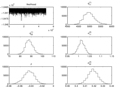
Figure 1: Histogram representations of marginal posterior probability densities of the 5 sought GP parameters generated by RW, given the training data.

We notice that the reciprocal correlation length scale $q^{(1)}_{11}$ is an order of magnitude higher than $q^{(1)}_{22}$; correlation between values of sampled function $\boldsymbol{\xi}(\cdot)$, computed at 2 different $s_{1}$ and the same $s_{2}$ then wanes more quickly in than correlation between sampled functions computed at same $s_{1}$ and different $S_{2}$ values. Here $\boldsymbol{s}=(s_{1},s_{2})^{T}$ and given that $\boldsymbol{S}$ is the location of the observer who observes the velocities of her neighbouring stars on a two-dimensional polar grid, $S_{1}$ is interpreted as the radial coordinate of the observer’s location in the Galaxy and $S_{2}$ is the observer’s angular coordinate. Then it appears that the velocities measured by observers at different radial coordinates, but at the same angle, are correlated over shorter length scales than velocities measured by observers at the same radial coordinate, but different angles. This is understood to be due to the astro-dynamical influences of the Galactic features included by Chakrabarty (2007) in the simulation that generates the training data that we use here. This simulation incorporates the joint dynamical effect of the Galactic spiral arms and the Galactic bar (of stars) that rotate at different frequencies (as per the astronomical model responsible for the generation of our training data), pivoted at the centre of the Galaxy. An effect of this joint handiwork of the bar and the spiral arms is to generate distinctive stellar velocity distributions at different radial (i.e. along the $S_{1}$ direction) coordinates, at the same angle ($s_{2}$). On the other hand, the stellar velocity distributions are more similar at different $S_{2}$ values, at the same $s_{1}$. This pattern is borne by Figure 9 of Chakrabarty (2004), in which the radial and angular variation of the standard deviations of these bivariate velocity distributions are plotted. Then it is understandable why the correlation length scales are shorter along the $S_{1}$ direction, than along the $S_{2}$ direction. Furthermore, for the correlation parameter $\rho$, physics suggests that the correlation will be zero among the two components of a velocity vector. These two components are after all, the components of the velocity vector in a 2-dimensional orthogonal basis. However, the MCMC chain shows that there is a small (negative) correlation between the two components of the stellar velocity vector.

4.1 Predicting $\boldsymbol{s}^{(test)}$

In the first method, we perform posterior sampling using RW, from the joint posterior probability density of all parameters (GP parameters as well as solar location vector), given test+training data. In Figure 2, we present the results of marginal posterior probability densities of the solar location coordinates $s^{(test)}_{1}$, $s^{(test)}_{2}$; $q_{11}^{1*}$ and $q_{22}^{1*}$ that get updated once the test data is added to augment the training data, and parameters $\sigma_{11}^{3*}$, $\sigma_{22}^{3*}$ and $\rho^{*}$. Traces of the likelihood and of the marginal posterior probabilities of all learnt parameters, given all data, are included in Figure 2 of the supplementary section. 95$\%$ HPD credible regions computed on each parameter in this inference scheme, are displayed in Table 1 of the supplementary section.

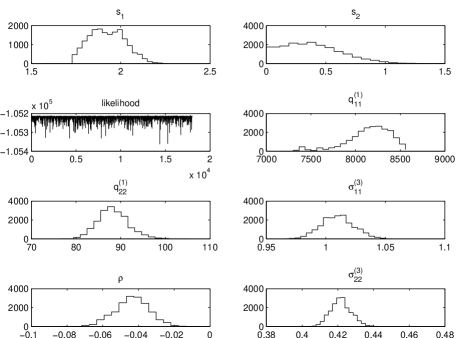
Figure 2: Histogram representations of marginal densities of $s^{(test)}_{1}$ and $s^{(test)}_{2}$ and the 5 GP parameters, from an MCMC chain run using test and training data.

We notice that the values of the inverse correlation length $q_{11}^{(1*)}$ has undergone substantial change with the introduction of the test data over the originally used training data–with the modal value increasing by a factor little less than 2. However $q_{22}^{(1*)}$ is almost the same as $q_{22}^{(1)}$. Thus, the introduction of the test data has caused shorter correlation length scales along the $S_{1}$ direction to be imposed, i.e. two observers seated at two different radial coordinates will find their observed velocities correlated over even shorter length scales–where such velocities are part of the augmented data set–than when the training data alone is used. However, there is very little effect of the added information from the test data on $q_{22}^{(1)}$. This indicates that while the generation of the velocities of nearby stars at a given observer angular coordinate was done well in the astronomical simulations performed by Chakrabarty (2007), the simulations failed to adequately capture the generation of stellar velocities at a given radial location. At least, on a comparative note, the simulations were a better representative of the test data measured by the Hipparcos satellite, when it came to the dependence of the velocities on observer angular coordinate, than on the observer radial coordinate.

The marginal distributions of $s_{1}^{(test)}$ indicates that the marginal is nearly bimodal, with modes at about 1.85 and 2 in model units. The distribution of $s_{2}^{(test)}$ on the other hand is quite strongly skewed towards values of $s_{2}^{(test)}\lesssim 1$ radians, i.e. $s_{2}^{(test)}\lesssim 57$ degrees, though the probability mass in this marginal density falls sharply after about 0.4 radians, i.e. about 23 degrees. These values tally quite well with previous work (Chakrabarty et al., 2015). In that earlier work, using the training data that we use in this work, (constructed using the the astronomical model $sp3bar3{\_}18$ discussed by Chakrabarty et al. (2015)), the marginal distribution of $s_{1}^{(test)}$ was learnt to be bimodal, with modes at about 1.85 and 2, in model units–this is what we find in our inference scheme. The distribution of $s_{2}^{(test)}$ found by (Chakrabarty et al., 2015) is however more constricted, with a sharp mode at about 0.32 radians (i.e. about 20 degrees). We do notice a mode at about this value in our inference, but unlike in the results of (Chakrabarty et al., 2015), we do not find the probability mass declining to low values beyond about 15 degrees. One possible reason for this lack of compatibility could be that in (Chakrabarty et al., 2015), the matrix of velocities $\boldsymbol{V}$ was vectorised, so that the training data then resembled a matrix, rather than a 3-tensor as we know it to be. Such vectorisation could have led to some loss of correlation information, leading to the results of (Chakrabarty et al., 2015).

When we predict $\boldsymbol{s}^{(test)}$ using test+training data, at the (modal values of the) GP parameters that are learnt from the training data, we generate samples from the posterior predictive of $\boldsymbol{s}^{(test)}$ (Equation 7) using RW. The marginal posterior predictive densities of $s_{1}^{(test)}$ and $s_{2}^{(test)}$ are shown in Figure 3. Trace of the likelihood and traces of the marginal posterior probability of the solar location parameters are shown in Figure 3 of the supplementary section.

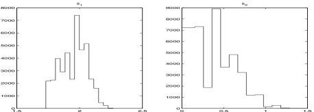
Figure 3: Histograms representing marginal posterior predictive probability densities of $s^{(test)}_{1}$ and $s^{(test)}_{2}$ given test+training data and GP parameters that are learnt given training data alone.

Results from the marginal predictive densities have similarities with the results from the marginals obtained in the other inference scheme, shown in Figure 2. Firstly, the modes of $s_{1}^{(test)}$ at about 1.85 and 2 are again noticed in Figure 3. The posterior predictive of $s_{2}^{(test)}$ is noticed to bear high probability mass in the [0,1] radian interval, though–as with the inference using the first method–here too, there is a decline after about 0.4 radians. However, the small dip noticed in Figure 2 at about 0.3 radians, is more pronounced here. In Chakrabarty et al. (2015), a secondary mode inward of about 0.3 radians, was missed. Thus, the vectorisation-based approach used by Chakrabarty et al. (2015) is found to have missed correlation information at low angles, i.e. very close to the long axis of the Galactic bar.

4.2 Astronomical implications

The radial coordinate of the observer in the Milky Way, i.e. the solar radial location is dealt with in model units, but will need to be scaled to real galactic unit of distance, which is kilo parsec (kpc). Now, from independent astronomical work, the radial location of the Sun is set as 8 kpc. Then our estimate of $S_{1}$ is to be scaled to 8 kpc, which gives 1 model unit of length to be $\displaystyle{\frac{8\mbox{kpc}}{\mbox{our estimate of\>\>}S_{1}}}$. Our main interest in learning the solar location is to find the frequency $\Omega_{bar}$ with which the Galactic bar is rotating, pivoted at the galactic centre, loosely speaking. Here $\Omega_{bar}=\displaystyle{\frac{v_{0}}{\mbox{1 model unit of length}}}$, where $v_{0}=220$ km/s (see Chakrabarty (2007) for details). The solar angular location being measured as the angular distance from the long-axis of the Galactic bar, our estimate of $S_{2}$ actually tells us the angular distance between the Sun-Galactic centre line and the long axis of the bar. These estimates are included in Table 2 of the supplementary section.

5 Conclusion

Our aim here is to advance a general methodology that allows for covariance modelling of high-dimensional data sets, to then be able to make an inverse learning of the input variable, given new or test data, when such data becomes available. To this effect, we make a simple application of the method, to thereafter check our results against results obtained previously, using the same data that we use. Our results compare favourably with previous work discussed in the literature (Chakrabarty et al., 2015).

Supplementary Section

Introduction In this supplement, there are two sections. The first section presents some of the results of our inference in 3 figures and 2 tables. The second section presents a schematic representation of the MCMC technique–namely the Random-Walk Metropolis-Hastings (RW)–that we have used in our work to perform posterior sampling.

1.   Results In our application we model the functional relationship between the 2-dimensional location vector $\boldsymbol{S}$ of the observer and the observable–which is 50$\times 2$ matrix $\boldsymbol{V}$ of 2-dimensional velocity vectors of 50 stars in the neighbourhood of a fiduciary observer.

Figure 4 presents trace of the likelihood of the training data given the unknown parameters of the GP that is used to model this functional relationship. Traces of the marginal posterior probability density of each of these GP parameters, given the training data, are also shown.

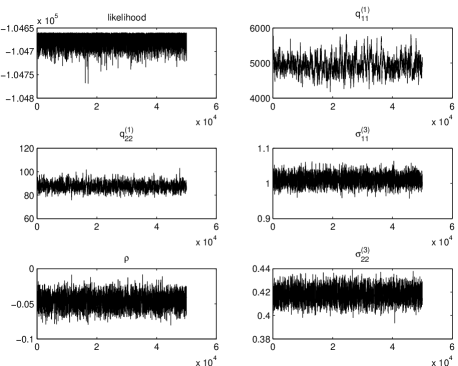
Figure 4: Traces of likelihood and marginal posterior density of GP parameters $q_{11}^{(1)},q_{22}^{(1)},\sigma_{11}^{(3)},\sigma_{22}^{(3)},\rho$ given training data.

Figure 5 presents trace of the likelihood of the training+test data given the unknown parameters of the GP and the location $\boldsymbol{s}^{(test)}=(s_{1}^{(test)},s_{2}^{(test)})^{T}$ of the Sun at which the test data is realised. Traces of the marginal posterior probability density of each of these GP parameters and the solar location, given the training+test data, are also shown. Details of this inference in discussed in Section 3.1 of the main paper.

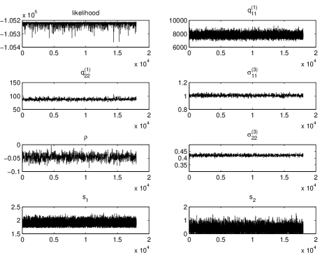
Figure 5: Traces of likelihood and marginal posterior density of parameters $s_{1}^{(test)},s_{2}^{(test)},q_{11}^{(1)},q_{22}^{(1)},\sigma_{11}^{(3)},\sigma_{22}^{(3)},\rho$ given training and test data.

Figure 6 presents traces of the posterior predictive probability of the location parameters $s_{1}^{(test)}$ and $s_{2}^{(test)}$ of the Sun, given all data and the modal values of parameters of the GP learnt using training data. Again, details of this inference is discussed in Section 3.1 of the main paper.

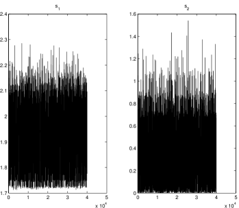
Figure 6: Traces of posterior predictive density of parameters $s_{1}^{(test)},s_{2}^{(test)}$ given training+test data and the modal values of the five GP parameters listed above, that were learnt from the training data alone.

Table 1: $95\%$ HPD on each learnt parameter, using the three inference schemes

Parameters	using only training data	sampling from posterior predictive	sampling from joint
$q^{(1)}_{11}$	[4572.4,5373.2]		[7566.8,8460.4]
$q^{(1)}_{22}$	[82.50,93.12]		[82.30,93.44]
$\sigma^{(3)}_{11}$	[0.9884,1.0337]		[0.9848,1.0310]
$\rho$	[-0.0627,-0.0310]		[-0.0620,-0.0304]
$\sigma^{(3)}_{22}$	[0.4087,0.4270]		[0.4116,0.4306]
$s_{1}$	-	[1.7496,2.0995]	[1.7547,2.0816]
$s_{2}$	-	[0.079,0.7609]	[0.0393,0.8165]

Table 2: $95\%$ HPD on each Galactic feature parameter learnt from the solar location coordinates learnt using the two predictive inference schemes listed above and as reported in a past paper for the same training and test data.

	$95\%$ HPD for $\Omega_{bar}$ (km/s/kpc)	for angular distance of bar to Sun (degrees)
from posterior predictive	$[48.11,57.73]$	$[4.53,43.62]$
from joint posterior	$[48.25,57.244]$	$[2.25,46.80]$
from Chakrabarty et. al (2015)	$[46.75,62.98]$	$[17.60,79.90]$

Table 1 summarises the 95$\%$ HPD credible regions of all learnt parameters, under the 3 different inference schemes, namely learning the GP parameters from training data alone; learning the GP and solar location parameters by sampling from the joint posterior probability density of all parameters, given all data; learning the solar location parameters by sampling from the posterior predictive of these, given all data and the modal values of the GP parameters learnt using training data alone.

Table 2 displays the Galactic feature parameters that derive frof the learnt solar location parameters, under the different inference schemes, namely, sampling from the joint posterior probability of all parameters given all data and from the posterior predictive of the solar location coordinates given all data and GP parameters already learnt from training data alone. The derived Galactic feature parameters are the the bar rotational frequency $\Omega_{bar}$ in the real astronomical units of km/s/kpc and the angular distance between the bar and the Sun, in degrees. The table also includes results from Chakrabarty et. al (2015), the reference for which is in the main paper.

2.   Random-Walk Metropolis-Hastings In this section we discuss the used MCMC technique–to be precise, RW. We base our discussion to the inference that is made using test+training data $\boldsymbol{D}^{*}$, on the unknown observer location coordinates $s_{1}^{(test)}$ and $s_{2}^{(test)}$ at which the test data is realised, the unknown correlation length scales $q_{11}^{1*}$ and $q_{22}^{1*}$ that parametrise the SQE parametrisation of the covariance matrix $\boldsymbol{\Sigma}_{1}$, the diagonal elements $\sigma_{11}^{(3)}$ and $\sigma_{22}^{(3)}$ of the covariance matrix $\boldsymbol{\Sigma}_{3}^{*}$ and the correlation between its non-diagonal elements, $\rho^{*}$. Here, the “^∗ superscript on the unknown parameters indicate their values that can be different as inferred using the augmented data $\boldsymbol{D}^{*}$, as distinguished from their value learnt with training data alone–which was marked with no asterisked superscript.

In the discussion of the inference scheme below, we refer to our 7 unknowns with the notation $\theta_{1},\ldots,\theta_{7}$.

1. Set the seed $\theta_{i}=\theta_{i}^{(0)}$, $i=1,\ldots,7$

2. In the $t$-th iteration, let current $\theta_{i}$ be $\theta_{i}^{(t)}$. Propose the value $\tilde{\theta_{i}}\sim{\cal N}(\theta_{i}^{(t-1)},\sigma_{i}^{2})$. Do this for each $i=1,\ldots,7$

3. Compute the acceptance ratio

   $$\alpha=\displaystyle{\frac{\pi(\tilde{\theta_{1}}\ldots\tilde{\theta_{7}}|\boldsymbol{D}^{*})}{\pi({\theta_{1}^{(t)}}\ldots\tilde{\theta_{7}^{(t)}}|\boldsymbol{D}^{*})}}$$

   Here the joint posterior $\pi(\cdot|\boldsymbol{D}^{*})$, of unknowns given the augmented data, is given in Equation 6 of the main paper.
   Generate uniform random number $u\sim{\cal U}[0,1]$. If $u\leq\alpha$, accept $\theta_{i}^{(t)}=\tilde{\theta_{i}}\>\forall i=1,\ldots,7$. If $u>\alpha$, set $\theta_{i}^{(t)}={\theta_{i}}^{(t-1)}\>\forall i$. Return to Step 2.

References

- Ramsay and Silverman (2014) J. Ramsay and B. W. (eds.) Silverman. Functional Data Analysis. Springer Series in Statistics. Springer, Philadelphia, 2014.
- Hofmann (2011) B. Hofmann. Ill-posedness and regularization of inverse problems—a review on mathematical methods. In The Inverse Problem. Symposium ad Memoriam H. v. Helmholtz, H. Lubbig (Ed)., pages 45–66. Akademie-Verlag, Berlin; VCH, Weinheim, 2011.
- Tarantola (2005) A. Tarantola. Inverse Problem Theory and Methods for Model Parameter Estimation. SIAM, Philadelphia, 2005.
- Gelman et al. (1995) A. Gelman, J. B. Carlin, H. S. Stern, and D. R. Rubin. Bayesian Data Analysis. Chapman and Hall, 1995. Second Edition.
- Neal (1998) R. M. Neal. Regression and classification using gaussian process priors (with discussion). In J. M. Bernardo et. al, editor, Bayesian Statistics 6, pages 475–501. Oxford University Press, 1998.
- Alquier et al. (2011) P. Alquier, E. Gautier, and G. (eds.) Stoltz. Inverse Problems and High-Dimensional Estimation. Number 203 in Lecture Notes in Statstics. Springer-Verlag, Berlin Heidelberg, 2011.
- Cavalier (2008) L. Cavalier. Nonparametric statistical inverse problems. Inverse Problems, 24(3):0340046, 2008.
- Zhao et al. (2014) Q. Zhao, G. Zhou, L. Zhang, and A. Cichocki. Tensor-variate gaussian processes regression and its application to video surveillance. In Acoustics, Speech and Signal Processing (ICASSP), 2014 IEEE International Conference on, pages 1265–1269. IEEE, 2014.
- Xu et al. (2012) Z. Xu, F. Yan, and A. Qi. Infinite tucker decomposition: Nonparametric bayesian models for multiway data analysis. In Proceedings of the 29th International Conference on Machine Learning, 2012.
- Hoff, P. D. (2011) Hoff, P. D. Separable covariance arrays via the Tucker product, with applications to multivariate relatonal data. Bayesian Analysis, 6(2):179–196, 2011.
- Hou et al. (2015) M. Hou, Y. Wang, and B. Chaib-draa. Online local gaussian process for tensor-variate regression: Application to fast reconstruction of limb movements from brain signal. In Acoustics, Speech and Signal Processing (ICASSP), 2015 IEEE International Conference on, pages 5490 – 5494. IEEE, 2015.
- Robert and Casella (2004) C. Robert and G. Casella. Monte Carlo Statistical Methods. Number 2 in Springer Texts in Statistics. Springer-Verlag, New York, 2004.
- Chakrabarty et al. (2015) Dalia Chakrabarty, M. Biswas, and S. Bhattacharya. Bayesian nonparametric estimation of milky way parameters using matrix-variate data, in a new gaussian process based method. Electronic Journal of Statistics, 9(1):1378–1403, 2015.
- Chakrabarty (2007) D. Chakrabarty. Phase Space around the Solar Neighbourhood. Astronomy & Astrophysics, 467:145, 2007.
- Aston and Kirch (2012) J. A. D. Aston and Claudia Kirch. Evaluating stationarity via change-point alternatives with applications to fmri data. Annals of Applied Statistics, 6(4):1906–1948, 2012.
- Knuth (1997) D. Knuth. The Art of Computer Programming: Seminumerical Algorithms. Addison-Wesley Longman Publishing Co., Boston, MA, USA, 1997.
- Chakrabarty (2004) D. Chakrabarty. Patterns in the outer parts of galactic disks. Monthly Notices of the Royal Astronomical Society, 352:427, 2004.