Optimality Conditions for Nonlinear Semidefinite Programming via Squared Slack Variables

Abstract

In this work, we derive second-order optimality conditions for nonlinear semidefinite programming (NSDP) problems, by reformulating it as an ordinary nonlinear programming problem using squared slack variables. We first consider the correspondence between Karush-Kuhn-Tucker points and regularity conditions for the general NSDP and its reformulation via slack variables. Then, we obtain a pair of “no-gap” second-order optimality conditions that are essentially equivalent to the ones already considered in the literature. We conclude with the analysis of some computational prospects of the squared slack variables approach for NSDP.

Keywords: Nonlinear semidefinite programming, squared slack variables, optimality conditions, second-order conditions.

1 Introduction

We consider the following nonlinear semidefinite programming (NSDP) problem:

$$\begin{array}[]{ll}\underset{x}{\mbox{minimize}}&f(x)\\ \mbox{subject to}&G(x)\in{\mathcal{S}^{m}_{+}},\end{array}$$ (P1)

where $f\colon\mathbb{R}^{n}\to\mathbb{R}$ and $G\colon\mathbb{R}^{n}\to\mathcal{S}^{m}$ are twice continuously differentiable functions, $\mathcal{S}^{m}$ is the linear space of all real symmetric matrices of dimension $m\times m$, and $\mathcal{S}^{m}_{+}$ is the cone of all positive semidefinite matrices in $\mathcal{S}^{m}$. Second-order optimality conditions for such problems were originally derived by Shapiro in [20]. It might be fair to say that the second-order analysis of NSDP problems is more intricated than its counterpart for classical nonlinear programming problems. That is one of the reasons why it is interesting to have alternative ways for obtaining optimality conditions for (P1); see the works by Forsgren [9] and Jarre [12]. In this work, we propose to use the squared slack variables approach for deriving these optimality conditions.

It is well-known that the squared slack variables can be used to transform a nonlinear programming (NLP) problem with inequality constraints into a problem with only equality constraints. For NLP problems, this technique was hardly considered in the literature because it increases the dimension of the problem and may lead to numerical instabilities [18]. However, recently, Fukuda and Fukushima [10] showed that the situation may change in the nonlinear second-order cone programming context. Here, we observe that the slack variables approach can be used also for NSDP problems, because, like the nonnegative orthant and the second-order cone, the cone of positive semidefinite matrices is also a cone of squares. More precisely, $\mathcal{S}^{m}_{+}$ can be represented as

$$\mathcal{S}^{m}_{+}=\{Z\circ Z\mid Z\in\mathcal{S}^{m}\},$$ (1.1)

where $\circ$ is the Jordan product associated with the space $\mathcal{S}^{m}$, which is defined as

$$W\circ Z:=\frac{WZ+ZW}{2}$$

for any $W,Z\in\mathcal{S}^{m}$. Note that actually $Z\circ Z=ZZ=Z^{2}$ for any $Z\in\mathcal{S}^{m}$.

The fact above allows us to develop the squared slack variables approach. In fact, by introducing a slack variable $Y\in\mathcal{S}^{m}$ in (P1), we obtain the following problem:

$$\begin{array}[]{ll}\underset{x,Y}{\mbox{minimize}}&f(x)\\ \mbox{subject to}&G(x)-Y\circ Y=0,\end{array}$$ (P2)

which is an NLP problem with only equality constraints. Note that if $(x,Y)\in\mathbb{R}^{n}\times\mathcal{S}^{m}$ is a global (local) minimizer of (P2), then $x$ is a global (local) minimizer of (P1). Moreover, if $x\in\mathbb{R}^{n}$ is a global (local) minimizer of (P1), then there exists $Y\in\mathcal{S}^{m}$ such that $(x,Y)$ is a global (local) minimizer of (P2). However, the relation between stationary points, or Karush-Kuhn-Tucker (KKT) points, of (P1) and (P2) is not so trivial. As in [10], we will take a closer look at this issue, and investigate also the relation between constraint qualifications for (P1) and (P2), using second-order conditions.

We remark that second-order conditions for these two problems are vastly different. While (P2) is a run-of-the-mill nonlinear programming problem, (P1) has nonlinear conic constraints, which are more difficult to deal with. Moreover, it is known that second-order conditions for NSDPs include an extra term, which takes into account the curvature of the cone. For more details, we refer to the papers of Kawasaki [13], Cominetti [7] and Shapiro [20]. The main objective of this work is to show that, under appropriate regularity conditions, second-order conditions for (P1) and (P2) are essentially the same. This suggests that the addition of the slack term already encapsulates most of the nonlinear structure of the cone. In the analysis, we also propose and use a sharp characterization of positive semidefiniteness that takes into account the rank information. We believe that such a characterization can be useful in other contexts as well.

Finally, we present results of some numerical experiments where NSDPs are reformulated as NLPs using slack variables. Note that we are not necessarily advocating the use of slack variables and we are, in fact, driven by curiosity about its computational prospects. Nevertheless, there are a couple of reasons why this could be interesting. First of all, conventional wisdom would say that using squared slack variables is not a good idea, but, in reality, even for linear SDPs there are good reasons to use such variables. In [5, 6], Burer and Monteiro transform a linear SDP $\inf\{\mathrm{tr}(CX)\mid\mathcal{A}X=b,X\in{\mathcal{S}^{m}_{+}}\}$ into $\inf\{\mathrm{tr}(CVV^{\top})\mid\mathcal{A}VV^{\top}=b\}$, where $V$ is a square matrix and $\mathrm{tr}$ denotes the trace map. The idea is to use a theorem, proven independently by Barvinok [1] and Pataki [16], which bounds the rank of possible optimal solutions. By doing so, it is possible to restrict $V$ to be a rectangular matrix instead of a square one, thereby reducing the number of variables. Another reason to use squared slack variables is that the reformulated NLP problem can be solved by efficient NLP solvers that are widely available. In fact, while there are a number of solvers for linear SDPs, as we move to the general nonlinear case, the situation changes drastically [22].

Throughout the paper, the following notations will be used. For $x\in\mathbb{R}^{s}$ and $Y\in\mathbb{R}^{\ell\times s}$, $x_{i}\in\mathbb{R}$ and $Y_{ij}\in\mathbb{R}$ denote the $i$th entry of $x$ and the $(i,j)$ entry ($i$th row and $j$th column) of $Y$, respectively. The identity matrix of dimension $\ell$ is denoted by $I_{\ell}$. The transpose, the Moore-Penrose pseudo-inverse, and the rank of $Y\in\mathbb{R}^{\ell\times s}$ are denoted by $Y^{\top}\in\mathbb{R}^{s\times\ell},Y^{\dagger}\in\mathbb{R}^{s\times\ell}$, and ${\mathrm{rank}\,}Y$, respectively. If $Y$ is a square matrix, its trace is denoted by $\mathrm{tr}(Y):=\sum_{i}Y_{ii}$. For square matrices $W$ and $Y$ of the same dimension, their inner product is denoted by $\langle W,Y\rangle:=\mathrm{tr}(W^{\top}Y)$. We will use the notation $Z\succeq 0$ for $Z\in{\mathcal{S}^{m}_{+}}$. In that case, we will denote by $\sqrt{Z}$ the positive semidefinite square root of $Z$, that is, $\sqrt{Z}$ satisfies $\sqrt{Z}\succeq 0$ and $\sqrt{Z}^{2}=Z$. For any function $\mathcal{P}\colon\mathbb{R}^{s+\ell}\to\mathbb{R}$, the gradient and the Hessian at $(x,y)\in\mathbb{R}^{s+\ell}$ with respect to $x$ are denoted by $\nabla_{x}\mathcal{P}(x,y)$ and $\nabla_{x}^{2}\mathcal{P}(x,y)$, respectively. Moreover, for any linear operator $\mathcal{G}\colon\mathbb{R}^{s}\to\mathcal{S}^{\ell}$ defined by $\mathcal{G}v=\sum_{i=1}^{s}v_{i}\mathcal{G}_{i}$ with $\mathcal{G}_{i}\in\mathcal{S}^{\ell}$, $i=1,\dots,s$, and $v\in\mathbb{R}^{s}$, the adjoint operator $\mathcal{G}^{*}:\mathcal{S}^{\ell}\to\mathbb{R}^{s}$ is defined by

$$\mathcal{G}^{*}Z=(\langle\mathcal{G}_{1},Z\rangle,\dots,\langle\mathcal{G}_{s},Z\rangle)^{\top},\quad Z\in\mathcal{S}^{\ell}.$$

Given a mapping $\mathcal{H}\colon\mathbb{R}^{s}\to\mathcal{S}^{\ell}$, its derivative at a point $x\in\mathbb{R}^{s}$ is denoted by $\nabla\mathcal{H}(x)\colon\mathbb{R}^{s}\to\mathcal{S}^{\ell}$ and defined by

$$\nabla\mathcal{H}(x)v=\sum_{i=1}^{s}v_{i}\frac{\partial\mathcal{H}(x)}{\partial x_{i}},\quad v\in\mathbb{R}^{s},$$

where $\partial\mathcal{H}(x)/\partial x_{i}\in\mathcal{S}^{\ell}$ are the partial derivative matrices. Finally, for a closed convex cone $K$, we will denote by $\mathrm{lin}\,K$ the largest subspace contained in $K$. Note that $\mathrm{lin}\,K=K\cap-K$.

The paper is organized as follows. In Section 2, we recall a few basic definitions concerning KKT points and second-order conditions for (P1) and (P2). We also give a sharp characterization of positive semidefiniteness. In Section 3, we prove that the original and the reformulated problems are equivalent in terms of KKT points, under some conditions. In Section 4, we establish the relation between constraint qualifications of those two problems. The analyses of second-order sufficient conditions and second-order necessary conditions are presented in Sections 5 and 6, respectively. In Section 7, we show some computational results. We conclude in Section 8, with final remarks and future works.

2 Preliminaries

2.1 A sharp characterization of positive semidefiniteness

It is a well-known fact that a matrix $\Lambda\in\mathcal{S}^{m}$ is positive semidefinite if and only if $\langle\Lambda,W^{2}\rangle\geq 0$ for all $W\in\mathcal{S}^{m}$. This statement is equivalent to the self-duality of the cone $S^{m}_{+}$. However, we get no information about the rank of $\Lambda$. In the next lemma, we give a new characterization of positive semidefinite matrices, which takes into account the rank information.

Lemma 2.1.

Let $\Lambda\in\mathcal{S}^{m}$. The following statements are equivalent:

1. $\Lambda\in{\mathcal{S}^{m}_{+}}$;

2. There exists $Y\in\mathcal{S}^{m}$ such that ${Y\circ\Lambda}=0$ and $Y\in\Phi(\Lambda)$, where

   $$\Phi(\Lambda):=\big{\{}Y\in\mathcal{S}^{m}\,|\,\langle{W\circ W},\Lambda\rangle>0\mbox{ for all }0\neq W\in\mathcal{S}^{m}\mbox{ with }{Y\circ W}=0\big{\}}.$$ (2.1)

For any $Y$ satisfying the conditions in $(ii)$, we have ${\mathrm{rank}\,}\Lambda=m-{\mathrm{rank}\,}Y$. Moreover, if $\sigma$ and $\sigma^{\prime}$ are nonzero eigenvalues of $Y$, then $\sigma+\sigma^{\prime}\neq 0$.

Proof.

Let us prove first that $(ii)$ implies $(i)$. Since the inner product is invariant under orthogonal transformations, we may assume without loss of generality that $Y$ is diagonal, i.e.,

$$Y=\begin{pmatrix}D&0\\ 0&0\end{pmatrix},$$

where $D$ is a $k\times k$ nonsingular diagonal matrix, and ${\mathrm{rank}\,}Y=k$. We partition $\Lambda$ in blocks in a similar way:

$$\Lambda=\begin{pmatrix}A&B\\ B^{\top}&C\end{pmatrix},$$

where $A\in\mathcal{S}^{k},B\in\mathbb{R}^{k\times(m-k)}$, and $C\in\mathcal{S}^{m-k}$. We will proceed by proving that $A=0$, $B=0$ and $C$ is positive definite.

First, observe that, by assumption,

$$0={Y\circ\Lambda}=\begin{pmatrix}{D\circ A}&DB/2\\ B^{\top}D/2&0\end{pmatrix}$$ (2.2)

holds. Since $D$ is nonsingular, this implies $B=0$. Now, let us prove that $A=0$. From (2.2) and the fact that $D$ is diagonal, we obtain

$$0=2({D\circ A})_{ij}=A_{ij}(D_{ii}+D_{jj}).$$ (2.3)

Again, because $D$ is nonsingular, it must be the case that all diagonal elements of $A$ should be zero. Now, suppose that $A_{ij}$ is nonzero for some $i$ and $j$, with $i\neq j$. In face of (2.3), this can only happen if $D_{ii}+D_{jj}=0$. Let us now consider the following matrix:

$$W=\begin{pmatrix}\widetilde{W}&0\\ 0&0\end{pmatrix}\in\mathcal{S}^{m},$$

where $\widetilde{W}\in\mathcal{S}^{k}$ is a submatrix containing only two nonzero elements, $\widetilde{W}_{ij}=1$ and $\widetilde{W}_{ji}=1$. Then, easy calculations show that ${\widetilde{W}\circ D}=0$, which also implies ${W\circ Y}=0$. Moreover, $\langle W\circ W,\Lambda\rangle=0$ because $\widetilde{W}^{2}={\widetilde{W}\circ\widetilde{W}}$ is the diagonal matrix having $1$ in the $(i,i)$ entry and $1$ in the $(j,j)$ entry, and since $A_{ii}$ and $A_{jj}$ are zero. We conclude that $Y\notin\Phi(\Lambda)$, contradicting the assumptions. So, it follows that $A$ must be zero. Similarly, we have that $D_{ii}+D_{jj}$ is never zero, which corresponds to the statement about eigenvalues $\sigma$ and $\sigma^{\prime}$ in the lemma. In fact, if $D_{ii}+D_{jj}$ is zero, then, by taking $W$ exactly as before, we have ${W\circ Y}=0$ and $\langle W\circ W,\Lambda\rangle=0$. Once again, this shows that $Y\notin\Phi(\Lambda)$, which is a contradiction.

It remains to show that $C$ is positive definite. Taking an arbitrary nonzero $\tilde{H}\in\mathcal{S}^{m-k}$, and defining

$$H=\begin{pmatrix}0&0\\ 0&\tilde{H}\end{pmatrix}\in\mathcal{S}^{m},$$

we easily obtain $H\circ Y=0$. Since $Y\in\Phi(\Lambda)$, we have $\langle H^{2},\Lambda\rangle>0$. But this shows that $\langle\tilde{H}^{2},C\rangle>0$, which implies that $C$ is positive definite. In particular, the rank of $\Lambda$ is equal to the rank of $C$, which is $m-\mathrm{rank}\,Y$.

Now, let us prove that $(i)$ implies $(ii)$. Similarly, we may assume $\Lambda=\bigl{(}\begin{smallmatrix}0&0\\ 0&C\end{smallmatrix}\bigr{)}$, with $C$ positive definite. Then, we can take $Y=\bigl{(}\begin{smallmatrix}E&0\\ 0&0\end{smallmatrix}\bigr{)}$, where $E$ is any positive definite matrix. It follows that any matrix $W\in\mathcal{S}^{m}$ satisfying ${Y\circ W}=0$ must have the shape $\bigl{(}\begin{smallmatrix}0&0\\ 0&F\end{smallmatrix}\bigr{)}$, for some matrix $F$. Since $C$ is positive definite, it is clear that $\langle{W\circ W},\Lambda\rangle>0$, whenever $W$ is nonzero. ∎

The statement about the sum of nonzero eigenvalues might seem innocuous at first, but it will be very useful in Section 5. In fact, the idea for this new characterization of positive semidefiniteness comes from the second-order conditions of (P2). For now, let us present another result that will be necessary. Given $A\in\mathcal{S}^{m}$, denote by $L_{A}\colon\mathcal{S}^{m}\to\mathcal{S}^{m}$ the linear operator defined by

$$L_{A}(E):={A\circ E}$$

for all $E\in\mathcal{S}^{m}$. There are many examples of invertible matrices $A$ for which the operator $L_{A}$ is not invertible. This is essentially due to the failure of the condition on the eigenvalues. The following proposition is well-known in the context of Euclidean Jordan algebra (see [21, Proposition 1]), but we include here a short-proof for completeness.

Proposition 2.2.

Let $A\in\mathcal{S}^{m}$. Then, $L_{A}$ is invertible if and only if $\sigma+\sigma^{\prime}\neq 0$ for every pair of eigenvalues $\sigma,\sigma^{\prime}$ of $A$; in this case, $A$ must be invertible.

Proof.

The statements in the proposition are all invariant under orthogonal transformations. Thus, we may assume without loss of generality that $A$ is already diagonalized, and so $A_{kk}$ is an eigenvalue of $A$ for every $k=1,\ldots,m$.

Let us show that the invertibility of $L_{A}$ implies the statement about the eigenvalues of $A$. We will do so by proving the contrapositive. Take $i$ and $j$ such that $A_{ii}+A_{jj}=0$. Let $W$ be such that all the entries are zero except for $W_{ij}=W_{ji}=1$. Then, we have ${A\circ W}=0$. This shows that the kernel of $L_{A}$ is non-trivial and consequently, $L_{A}$ is not invertible.

Reciprocally, since we assume that $A$ is diagonal, for every $W\in\mathcal{S}^{m}$, we have $2(L_{A}(W))_{ij}=W_{ij}(A_{ii}+A_{jj})$ for all $i$ and $j$. Due to the fact that $A_{ii}+A_{jj}$ is never zero, the kernel of $L_{A}$ must only contain the zero matrix. Hence $L_{A}$ is invertible, and the result follows. ∎

In view of Proposition 2.2, the matrix $D$ which appears in the proof of Lemma 2.1 is such that $L_{D}$ is invertible. This will play an important role when we discuss the relation between the second-order sufficient conditions of problems (P1) and (P2).

2.2 KKT conditions and constraint qualifications

Now, let us consider the following lemma, which will allow us to present appropriately the KKT conditions of problems (P1) and (P2).

Lemma 2.3.

The following statements hold.

• For any matrices $A,B\in\mathbb{R}^{m\times m}$, let $\varphi\colon\mathbb{R}^{m\times m}\to\mathbb{R}$ be defined by $\varphi(Z):=\mathrm{tr}(Z^{\top}AZB)$. Then, we have $\nabla\varphi(Z)=AZB+A^{\top}ZB^{\top}$.

• For any matrix $A\in\mathcal{S}^{m}$, let $\varphi\colon\mathcal{S}^{m}\to\mathbb{R}$ be defined by $\varphi(Z):=\langle Z\circ Z,A\rangle$. Then, we have $\nabla\varphi(Z)=2{Z\circ A}$.

• For any matrix $A\in\mathbb{R}^{m\times m}$ and function $\theta\colon\mathbb{R}^{n}\to\mathcal{S}^{m}$, let $\psi\colon\mathbb{R}^{n}\to\mathbb{R}$ be defined by $\psi(x)=\langle\theta(x),A\rangle$. Then, we have $\nabla\psi(x)=\nabla\theta(x)^{*}A$.

• Let $A,B\in\mathcal{S}^{m}$. Then, they commute, i.e., $AB=BA$, if and only if $A$ and $B$ are simultaneously diagonalizable by an orthogonal matrix, i.e., there exists an orthogonal matrix $Q$ such that $QAQ^{\top}$ and $QBQ^{\top}$ are diagonal.

• Let $A,B\in\mathcal{S}^{m}_{+}$. Then, $AB=0$ if and only if $\langle A,B\rangle=0$.

Proof.

(a) See [2, Section 10.7].

(b) Note that $\varphi(Z)=\langle{Z\circ Z},\Lambda\rangle=\frac{1}{2}\langle ZZ^{\top},A\rangle+\frac{1}{2}\langle Z^{\top}Z,A\rangle=\frac{1}{2}\mathrm{tr}(ZZ^{\top}A)+\frac{1}{2}\mathrm{tr}(Z^{\top}ZA)=\frac{1}{2}\mathrm{tr}(Z^{\top}AZ)+\frac{1}{2}\mathrm{tr}(Z^{\top}ZA)$. Let $\varphi_{1}(Z)=\mathrm{tr}(Z^{\top}AZ)$ and $\varphi_{2}(Z)=\mathrm{tr}(Z^{\top}ZA)$. Then, from item (a), we have $\nabla\varphi_{1}(Z)=AZ+A^{\top}Z$ and $\nabla\varphi_{2}(Z)=ZA+ZA^{\top}$. Taking into account the symmetry of $A$, we have $\nabla\varphi_{1}(Z)=2AZ$ and $\nabla\varphi_{2}(Z)=2ZA$. Hence we have $\nabla\varphi(Z)=\frac{1}{2}\nabla\varphi_{1}(Z)+\frac{1}{2}\nabla\varphi_{2}(Z)=2{A\circ Z}$.

(c) Observe that $\psi(x)=\langle\theta(x),A\rangle=\mathrm{tr}(\theta(x)A)=\sum_{i,j}\theta(x)_{ij}A_{ij}$ for any $x\in\mathbb{R}^{n}$. Then, we have

$$\nabla\psi(x)=\left(\begin{array}[]{c}\sum_{i,j}(\partial\theta(x)_{ij}/\partial x_{1})A_{ij}\\ \vdots\\ \sum_{i,j}(\partial\theta(x)_{ij}/\partial x_{n})A_{ij}\end{array}\right)=\left(\begin{array}[]{c}\langle\partial\theta(x)/\partial x_{1},A\rangle\\ \vdots\\ \langle\partial\theta(x)/\partial x_{n},A\rangle\\ \end{array}\right)=\nabla\theta(x)^{*}A,$$

where the last equality follows from the definition of adjoint operator.

(d) See [2, Section 8.17].

(e) See [2, Section 8.12]. ∎

We can now recall the KKT conditions of problems (P1) and (P2). First, define the Lagrangian function $L\colon\mathbb{R}^{n}\times\mathcal{S}^{m}\to\mathbb{R}$ associated with problem (P1) as

$$L(x,\Lambda):=f(x)-\langle G(x),\Lambda\rangle.$$

We say that $(x,\Lambda)\in\mathbb{R}^{n}\times\mathcal{S}^{m}$ is a KKT pair of problem (P1) if the following conditions are satisfied:

$$\nabla f(x)-\nabla G(x)^{*}\Lambda=0,$$ (P1.1)

$$\Lambda\succeq 0,$$ (P1.2)

$$G(x)\succeq 0,$$ (P1.3)

$${\Lambda\circ G(x)}=0,$$ (P1.4)

where, from Lemma 2.3(c), we have $\nabla f(x)-\nabla G(x)^{*}\Lambda=\nabla_{x}L(x,\Lambda)$. Applying the trace map on both sides of (P1.4), we see that condition (P1.4) is equivalent to $\langle\Lambda,G(x)\rangle=0$. This result, together with the fact that $\Lambda\succeq 0$ and $G(x)\succeq 0$, shows that (P1.4) is also equivalent to $\Lambda G(x)=0$, by Lemma 2.3(e). Moreover, the equality (P1.4) implies that $\Lambda$ and $G(x)$ commute, which means, by Lemma 2.3(d), that they are simultaneously diagonalizable by an orthogonal matrix. The following definition is also well-known.

Definition 2.4.

If $(x,\Lambda)\in\mathbb{R}^{n}\times\mathcal{S}^{m}$ is a KKT pair of (P1) such that

$${\mathrm{rank}\,}G(x)+{\mathrm{rank}\,}\Lambda=m,$$

then $(x,\Lambda)$ is said to satisfy the strict complementarity condition.

As for the equality constrained NLP problem (P2), we observe that $(x,Y,\Lambda)\in\mathbb{R}^{n}\times\mathcal{S}^{m}\times\mathcal{S}^{m}$ is a KKT triple if the conditions below are satisfied:

$$\nabla_{(x,Y)}\mathcal{L}(x,Y,\Lambda) =0,$$

$$G(x)-Y\circ Y =0,$$

where $\mathcal{L}\colon\mathbb{R}^{n}\times\mathcal{S}^{m}\times\mathcal{S}^{m}\to\mathbb{R}$ is the Lagrangian function associated with (P2), which is given by

$$\mathcal{L}(x,Y,\Lambda):=f(x)-\langle G(x)-Y\circ Y,\Lambda\rangle.$$

From Lemma 2.3(b),(c), these conditions can be written as follows:

$$\nabla f(x)-\nabla G(x)^{*}\Lambda=0,$$ (P2.1)

$${\Lambda\circ Y}=0,$$ (P2.2)

$$G(x)-Y\circ Y=0.$$ (P2.3)

For problem (P1), we say that the Mangasarian-Fromovitz constraint qualification (MFCQ) holds at a point $x$ if there exists some $d\in\mathbb{R}^{n}$ such that

$$G(x)+\nabla G(x)d\in\mathrm{int}\,{\mathcal{S}^{m}_{+}},$$

where $\mathrm{int}\,{\mathcal{S}^{m}_{+}}$ denotes the interior of ${\mathcal{S}^{m}_{+}}$, that is, the set of symmetric positive definite matrices. If $x$ is a local minimum for (P1), MFCQ ensures the existence of a Lagrange multiplier $\Lambda$ and that the set of multipliers is bounded. A more restrictive assumption is the nondegeneracy condition discussed in [20], where it is presented in terms of a transversality condition on the map $G$. However, at the end, it boils down to the following condition.

Definition 2.5.

Suppose that $(x,\Lambda)\in\mathbb{R}^{n}\times\mathcal{S}^{m}$ is a KKT pair of (P1) such that

$$\mathcal{S}^{m}=\mathrm{lin}\,{\mathcal{T}_{{\mathcal{S}^{m}_{+}}}(G(x))}+\mathrm{Im}\,\nabla G(x),$$

where $\mathrm{Im}\,\nabla G(x)$ denotes the image of the linear map $\nabla G(x)$, ${\mathcal{T}_{{\mathcal{S}^{m}_{+}}}(G(x))}$ denotes the tangent cone of $\mathcal{S}^{m}_{+}$ at $G(x)$, and $\mathrm{lin}\,{\mathcal{T}_{{\mathcal{S}^{m}_{+}}}(G(x))}$ is the lineality space of the tangent cone ${\mathcal{T}_{{\mathcal{S}^{m}_{+}}}(G(x))}$, i.e., $\mathrm{lin}\,{\mathcal{T}_{{\mathcal{S}^{m}_{+}}}(G(x))}={\mathcal{T}_{{\mathcal{S}^{m}_{+}}}(G(x))}\cap-{\mathcal{T}_{{\mathcal{S}^{m}_{+}}}(G(x))}$ (see, for instance, the observations on page 310 in [20]). Then, $(x,\Lambda)$ is said to satisfy the nondegeneracy condition.

A good thing about the nondegeneracy condition is that it ensures that $\Lambda$ is unique.

For problem (P2), a common constraint qualification is the linear independence constraint qualification (LICQ), which simply requires that the gradients of the constraints be linearly independent. In Section 4, we will show that LICQ and the nondegeneracy are essentially equivalent.

2.3 Second-order conditions

Since (P2) is just an ordinary equality constrained nonlinear program, second-order sufficient conditions are well-known and can be written as follows.

Proposition 2.6.

Let $(x,Y,\Lambda)\in\mathbb{R}^{n}\times\mathcal{S}^{m}\times\mathcal{S}^{m}$ be a KKT triple of problem (P2). The second-order sufficient condition (SOSC-NLP) holds if

$$\langle\nabla_{x}^{2}L(x,\Lambda)v,v\rangle+2\langle{W\circ W},\Lambda\rangle>0$$ (2.4)

for every nonzero $(v,W)\in\mathbb{R}^{n}\times\mathcal{S}^{m}$ such that $\nabla G(x)v-2{Y\circ W}=0$.

Proof.

The second-order sufficient condition for (P2) holds if

$$\langle\nabla_{(x,Y)}^{2}\mathcal{L}(x,Y,\Lambda)(v,W),(v,W)\rangle>0$$

for every nonzero $(v,W)\in\mathbb{R}^{n}\times\mathcal{S}^{m}$ such that $\nabla G(x)v-2{Y\circ W}=0$; see [3, Section 3.3] or [15, Theorem 12.6]. Since

$$\langle\nabla_{(x,Y)}^{2}\mathcal{L}(x,Y,\Lambda)(v,W),(v,W)\rangle=\langle\nabla_{x}^{2}L(x,\Lambda)v,v\rangle+2\langle{W\circ W},\Lambda\rangle,$$

we have the desired result. ∎

Similarly, we have the following second-order necessary condition. Note that we require the LICQ to hold.

Proposition 2.7.

Let $(x,Y)$ be a local minimum for (P2) and $(x,Y,\Lambda)\in\mathbb{R}^{n}\times\mathcal{S}^{m}\times\mathcal{S}^{m}$ be a KKT triple such that LICQ holds. Then, the following second-order necessary condition (SONC-NLP) holds:

$$\langle\nabla_{x}^{2}L(x,\Lambda)v,v\rangle+2\langle{W\circ W},\Lambda\rangle\geq 0$$ (2.5)

for every $(v,W)\in\mathbb{R}^{n}\times\mathcal{S}^{m}$ such that $\nabla G(x)v-2{Y\circ W}=0$.

Proof.

See [15, Theorem 12.5]. ∎

Second-order conditions for (P1) are a more delicate matter. Let $(x,\Lambda)$ be a KKT pair of (P1). It is true that a sufficient condition for optimality is that the Hessian of the Lagrangian be positive definite over the set of critical directions. However, replacing “positive definite” by “positive semidefinite” does not yield a necessary condition. Therefore, it seems that there is a gap between necessary and sufficient conditions. In order to close the gap, it is essential to add an additional term to the Hessian of the Lagrangian. For the theory behind this see, for instance, the papers by Kawasaki [13], Cominetti [7], and Bonnans, Cominetti and Shapiro [4]. The condition below was obtained by Shapiro in [20] and it is sufficient for $(x,\Lambda)$ to be a local minimum, see Theorem 9 therein.

Proposition 2.8.

Let $(x,\Lambda)\in\mathbb{R}^{n}\times\mathcal{S}^{m}$ be a KKT pair of problem (P1) satisfying strict complementarity and the nondegeneracy condition. The second-order sufficient condition (SOSC-SDP) holds if

$$\langle(\nabla_{x}^{2}L(x,\Lambda)+H(x,\Lambda))d,d\rangle>0$$ (2.6)

for all nonzero $d\in\mathcal{C}(x)$, where

$$\mathcal{C}(x):=\left\{d\in\mathbb{R}^{n}\,\middle|\,\nabla G(x)d\in{\mathcal{T}_{{\mathcal{S}^{m}_{+}}}(G(x))},\langle\nabla f(x),d\rangle=0\right\}$$

is the critical cone at $x$, and $H(x,\Lambda)\in\mathcal{S}^{m}$ is a matrix with elements

$$H(x,\Lambda)_{ij}:=2\,\mathrm{tr}\left(\frac{\partial G(x)}{\partial x_{i}}G(x)^{\dagger}\frac{\partial G(x)}{\partial x_{j}}\Lambda\right)$$ (2.7)

for $i,j=1,\ldots,n$. In this case, $(x,\Lambda)$ is a local minimum for (P1). Conversely, if $x$ is a local minimum for (P1) and $(x,\Lambda)$ is a KKT pair satisfying strict complementarity and nondegeneracy, then the following second-order necessary condition (SONC-SDP) holds:

$$\langle(\nabla_{x}^{2}L(x,\Lambda)+H(x,\Lambda))d,d\rangle\geq 0$$ (2.8)

for all $d\in\mathcal{C}(x)$.

3 Equivalence between KKT points

Let us now establish the relation between KKT points of the original problem (P1) and its reformulation (P2). We start with the following simple implication.

Proposition 3.1.

Let $(x,\Lambda)\in\mathbb{R}^{n}\times\mathcal{S}^{m}$ be a KKT pair of problem (P1). Then, there exists $Y\in\mathcal{S}^{m}$ such that $(x,Y,\Lambda)$ is a KKT triple of (P2).

Proof.

Let $Y\in{\mathcal{S}^{m}_{+}}$ be the positive semidefinite matrix satisfying $G(x)={Y\circ Y}$. Let us show that $(x,Y,\Lambda)$ is a KKT triple of (P2). The conditions (P2.1) and (P2.3) are immediate. We need to show that (P2.2) holds.

Recall that (P1.4) along with (P1.2) and (P1.3) implies $G(x)\Lambda=0$, due to Lemma 2.3(e). It means that every column of $\Lambda$ lies in the kernel of $G(x)$. However, $G(x)$ and $Y$ share exactly the same kernel, since $G(x)=Y^{2}$. It follows that $Y\Lambda=0$, so that ${Y\circ\Lambda}=0$.

∎

The converse is not always true. That is, even if $(x,Y,\Lambda)$ is a KKT triple of (P2), $(x,\Lambda)$ may fail to be a KKT pair of (P1), since $\Lambda$ need not be positive semidefinite. This, however, is the only obstacle for establishing equivalence.

Proposition 3.2.

If $(x,Y,\Lambda)\in\mathbb{R}^{n}\times\mathcal{S}^{m}\times\mathcal{S}^{m}$ is a KKT triple of (P2) such that $\Lambda$ is positive semidefinite, then $(x,\Lambda)$ is a KKT pair of (P1).

Proof.

The only condition that remains to be verified is (P1.4). Due to (P2.2), we have

$$0 =\langle Y,{Y\circ\Lambda}\rangle=\langle{Y\circ Y},\Lambda\rangle=\langle G(x),\Lambda\rangle.$$

Since $G(x)$ and $\Lambda$ are both positive semidefinite, we must have ${G(x)\circ\Lambda}=0$. ∎

The previous proposition leads us to consider conditions which ensure that $\Lambda$ is positive semidefinite. It turns out that if the second-order sufficient condition for (P2) is satisfied at $(x,Y,\Lambda)$, then $\Lambda$ is positive semidefinite. In fact, a weaker condition is enough to ensure positive semidefiniteness.

Proposition 3.3.

Suppose that $(x,Y,\Lambda)\in\mathbb{R}^{n}\times\mathcal{S}^{m}\times\mathcal{S}^{m}$ is a KKT triple of (P2) such that $Y\in\Phi(\Lambda)$, where $\Phi(\Lambda)$ is defined by (2.1), that is,

$$\langle{W\circ W},\Lambda\rangle>0$$ (3.1)

for every nonzero $W\in\mathcal{S}^{m}$ such that ${Y\circ W}=0$. Then $(x,\Lambda)$ is a KKT pair of (P1) satisfying strict complementarity.

Proof.

Due to Lemma 2.1, $\Lambda$ is positive semidefinite and ${\mathrm{rank}\,}Y=m-{\mathrm{rank}\,}\Lambda$. Now, since $G(x)=Y^{2}$, we have ${\mathrm{rank}\,}G(x)={\mathrm{rank}\,}Y$. Therefore $(x,\Lambda)$ must satisfy the strict complementarity condition. ∎

Corollary 3.4.

Suppose that SOSC-NLP is satisfied at a KKT triple $(x,Y,\Lambda)\in\mathbb{R}^{n}\times\mathcal{S}^{m}\times\mathcal{S}^{m}$. Then $(x,\Lambda)$ is a KKT pair for (P1) which satisfies the strict complementarity condition.

Proof.

If we take $v=0$ in the definition of SOSC-NLP, we obtain $Y\in\Phi(\Lambda)$. So, the result follows from Proposition 3.3. ∎

The next result is a refinement of Proposition 3.1.

Proposition 3.5.

Suppose that $(x,\Lambda)\in\mathbb{R}^{n}\times\mathcal{S}^{m}$ is a KKT pair of (P1) which satisfies the strict complementarity condition. Then there exists some $Y\in\Phi(\Lambda)$ such that $(x,Y,\Lambda)$ is a KKT triple of (P2).

Proof.

Without loss of generality, we may assume that $G(x)$ has the shape $\bigl{(}\begin{smallmatrix}A&0\\ 0&0\end{smallmatrix}\bigr{)}$, where $A\in{\mathcal{S}^{k}_{+}}$ and $k={\mathrm{rank}\,}G(x)$. Since $G(x)$ and $\Lambda$ are both positive semidefinite, the condition ${G(x)\circ\Lambda}=0$ is equivalent to $G(x)\Lambda=0$. It follows that $\Lambda$ has the shape $\bigl{(}\begin{smallmatrix}0&0\\ 0&C\end{smallmatrix}\bigr{)}$ for some matrix $C\in{\mathcal{S}^{m-k}_{+}}$. However, strict complementarity holds only if $C$ is positive definite. Therefore, it is enough to pick $Y$ to be the positive semidefinite matrix satisfying $Y^{2}=G(x)$.

Finally, note that if $W=\bigl{(}\begin{smallmatrix}W_{1}&W_{2}\\ W_{2}^{\top}&W_{3}\end{smallmatrix}\bigr{)}$, with $W\in\mathcal{S}^{m},W_{1}\in\mathcal{S}^{k}$, $W_{2}\in\mathbb{R}^{k\times(m-k)}$, $W_{3}\in\mathcal{S}^{m-k}$, then the condition ${Y\circ W}=0$ together with Proposition 2.2 implies $W_{1}=0$, $W_{2}=0$. Since $C$ is positive definite, we must have $\langle\Lambda,{W\circ W}\rangle>0$, if $W\neq 0$. From (2.1), this shows that $Y\in\Phi(\Lambda)$. ∎

4 Relations between constraint qualifications

In this section, we shall show that the nondegeneracy in Definition 2.5 is essentially equivalent to LICQ for (P2). In [20], Shapiro mentions that the nondegeneracy condition for (P1) is an analogue of LICQ, but he also states that the analogy is imperfect. For instance, when $G(x)$ is diagonal, (P1) naturally becomes an NLP, since the semidefiniteness constraint is reduced to the nonnegativity of the diagonal elements. However, even in that case, LICQ and the nondegeneracy in Definition 2.5 might not be equivalent (see page 309 of [20]). In this sense, it is interesting to see whether a correspondence between the conditions can be established when (P1) is reformulated as (P2). Before that, we recall some facts about the geometry of the cone of positive semidefinite matrices.

Let $A\in{\mathcal{S}^{m}_{+}}$ and let $U$ be an $m\times k$ matrix whose columns form a basis for the kernel of $A$. Then, the tangent cone of ${\mathcal{S}^{m}_{+}}$ at $A$ is written as

$${\mathcal{T}_{{\mathcal{S}^{m}_{+}}}(A)}=\{E\in\mathcal{S}^{m}\mid U^{\top}EU\in{\mathcal{S}^{k}_{+}}\}$$

(see [17] or [20, Equation 26]). For example, if $A$ can be written as $\bigl{(}\begin{smallmatrix}D&0\\ 0&0\end{smallmatrix}\bigr{)}$, where $D$ is positive definite, then the matrices in ${\mathcal{T}_{{\mathcal{S}^{m}_{+}}}(A)}$ have the shape $\bigl{(}\begin{smallmatrix}C&F\\ F^{\top}&H\end{smallmatrix}\bigr{)}$, where the only restriction is that $H$ should be positive semidefinite.

Our first step is to notice that nondegeneracy implies that the only matrix which is orthogonal to both $\mathrm{lin}\,{\mathcal{T}_{{\mathcal{S}^{m}_{+}}}(G(x))}$ and $\mathrm{Im}\,\nabla G(x)$ is the trivial one, i.e.,

$$W\in(\mathrm{lin}\,{\mathcal{T}_{{\mathcal{S}^{m}_{+}}}(G(x))})^{\perp}\text{ and }\nabla G(x)^{*}W=0\quad\Rightarrow\quad W=0,$$ (Nondegeneracy)

where $\perp$ denotes the orthogonal complement.

On the other hand, the LICQ constraint qualification for (P2) holds at a feasible point $(x,Y)$ if the linear function which maps $(v,W)$ to $\nabla G(x)v-2{W\circ Y}$ is surjective. This happens if and only if the adjoint map has trivial kernel. The adjoint map takes $W\in\mathcal{S}^{m}$ and maps it to $(\nabla G(x)^{*}W,-2{W\circ Y})$. So the surjectivity assumption amounts to requiring that every $W$ which satisfies both $\nabla G(x)^{*}W=0$ and ${W\circ Y}=0$ must actually be $0$, that is,

$${W\circ Y}=0\text{ and }\nabla G(x)^{*}W=0\quad\Rightarrow\quad W=0.$$ (LICQ)

The subspaces $\ker L_{Y}=\{W\mid{Y\circ W}=0\}$ and $(\mathrm{lin}\,{\mathcal{T}_{{\mathcal{S}^{m}_{+}}}(G(x))})^{\perp}$ are closely related. The next proposition clarifies this connection.

Proposition 4.1.

Let $V=Y^{2}$, then $(\mathrm{lin}\,{\mathcal{T}_{{\mathcal{S}^{m}_{+}}}(V)})^{\perp}\subseteq\ker L_{Y}$. If $Y$ is positive semidefinite, then $\ker L_{Y}\subseteq(\mathrm{lin}\,{\mathcal{T}_{{\mathcal{S}^{m}_{+}}}(V)})^{\perp}$ as well.

Proof.

Note that if $Q$ is an orthogonal matrix, then ${\mathcal{T}_{{\mathcal{S}^{m}_{+}}}(Q^{\top}VQ)}=Q^{\top}{\mathcal{T}_{{\mathcal{S}^{m}_{+}}}(V)}Q$. The same is true for $\ker L_{Y}$, i.e., $\ker L_{Q^{\top}YQ}=Q^{\top}\ker L_{Y}Q$. So, without loss of generality, we may assume that $Y$ is diagonal and that

$$Y=\begin{pmatrix}D&0\\ 0&0\end{pmatrix},$$

where $D$ is an $r\times r$ nonsingular diagonal matrix. Then, we have

$${\mathcal{T}_{{\mathcal{S}^{m}_{+}}}(V)} =\left\{\begin{pmatrix}A&B\\ B^{\top}&C\end{pmatrix}\,\middle|\,A\in\mathcal{S}^{r},B\in\mathbb{R}^{r\times(m-r)},C\in{\mathcal{S}^{m-r}_{+}}\right\},$$

$$\mathrm{lin}\,{\mathcal{T}_{{\mathcal{S}^{m}_{+}}}(V)} =\left\{\begin{pmatrix}A&B\\ B^{\top}&0\end{pmatrix}\,\middle|\,A\in\mathcal{S}^{r},B\in\mathbb{R}^{r\times(m-r)}\right\},$$

$$(\mathrm{lin}\,{\mathcal{T}_{{\mathcal{S}^{m}_{+}}}(V)})^{\perp} =\left\{\begin{pmatrix}0&0\\ 0&C\end{pmatrix}\,\middle|\,C\in\mathcal{S}^{m-r}\right\}.$$

This shows that every matrix $Z\in(\mathrm{lin}\,{\mathcal{T}_{{\mathcal{S}^{m}_{+}}}(V)})^{\perp}$ satisfies $YZ=0$ and therefore lies in $\ker L_{Y}$. Now, the kernel of $L_{Y}$ can be described as follows:

$$\ker L_{Y}=\left\{\begin{pmatrix}A&0\\ 0&C\end{pmatrix}\,\middle|\,{A\circ D}=0,C\in\mathcal{S}^{m-r}\right\}.$$

If $Y$ is positive semidefinite, then $D$ is positive definite and the operator $L_{D}$ is nonsingular. Hence ${A\circ D}=0$ implies $A=0$. In this case, $\ker L_{Y}$ coincides with $(\mathrm{lin}\,{\mathcal{T}_{{\mathcal{S}^{m}_{+}}}(V)})^{\perp}$. ∎

Corollary 4.2.

If $(x,Y)\in\mathbb{R}^{n}\times\mathcal{S}^{m}$ satisfies LICQ for the problem (P2), then nondegeneracy is satisfied at $x$ for (P1). On the other hand, if $x$ satisfies nondegeneracy and if $Y=\sqrt{G(x)}$, then $(x,Y)$ satisfies LICQ for (P2).

Proof.

It follows easily from Proposition 4.1. ∎

5 Analysis of second-order sufficient conditions

In this section, we examine the relations between KKT points of (P1) and (P2) that satisfy second-order sufficient conditions.

Proposition 5.1.

Suppose that $(x,Y,\Lambda)\in\mathbb{R}^{n}\times\mathcal{S}^{m}\times\mathcal{S}^{m}$ is a KKT triple of (P2) satisfying SOSC-NLP. Then $(x,\Lambda)$ is a KKT pair of (P1) that satisfies strict complementarity and (2.6). If additionally, $(x,Y,\Lambda)$ satisfies LICQ for (P2) or $(x,\Lambda)$ satisfies nondegeneracy for (P1), then $(x,\Lambda)$ satisfies SOSC-SDP as well.

Proof.

In Corollary 3.4, we have already shown that $(x,\Lambda)$ is a KKT pair of (P1) and strict complementarity is satisfied. In addition, if $(x,Y,\Lambda)$ satisfies LICQ for (P2), then Corollary 4.2 ensures that $(x,\Lambda)$ satisfies nondegeneracy for (P1). It only remains to show that (2.6) is also satisfied. To this end, consider an arbitrary nonzero $d\in\mathbb{R}^{n}$ such that $\nabla G(x)d\in{\mathcal{T}_{{\mathcal{S}^{m}_{+}}}(G(x))}$ and $\langle\nabla f(x),d\rangle=0$. We are thus required to show that

$$\langle(\nabla_{x}^{2}L(x,\Lambda)+H(x,\Lambda))d,d\rangle>0,$$ (5.1)

where $H(x,\Lambda)$ is defined in (2.7). A first observation is that, due to (P1.1), we have $\langle\nabla G(x)d,\Lambda\rangle=\langle d,\nabla G(x)^{*}\Lambda\rangle=\langle d,\nabla f(x)\rangle=0$, that is, $\nabla G(x)d\in\{\Lambda\}^{\perp}$. We recall that $H(x,\Lambda)$ satisfies

$$\langle H(x,\Lambda)d,d\rangle=2\langle\Lambda,(\nabla G(x)d)^{\top}G^{\dagger}(x)\nabla G(x)d\rangle.$$ (5.2)

The strategy here is to first identify the shape and properties of several matrices involved, before showing that (5.1) holds. Without loss of generality, we may assume that $G(x)$ is diagonal, i.e.,

$$G(x)=\begin{pmatrix}D&0\\ 0&0\end{pmatrix},$$

where $D$ is a $k\times k$ diagonal positive definite matrix. We also have

$$Y=\begin{pmatrix}E&0\\ 0&0\end{pmatrix},$$

with $E$ an invertible diagonal matrix such that $E^{2}=D$. Since SOSC-NLP holds, considering $v=0$ in (2.4), we obtain $\langle{W\circ W},\Lambda\rangle>0$ for all nonzero $W\in\mathcal{S}^{m}$ such that ${W\circ Y}=0$, which, by (2.1), shows that $Y\in\Phi(\Lambda)$. From (P2.2), we also have ${Y\circ\Lambda}=0$. Thus, Lemma 2.1 ensures that every pair $\sigma,\sigma^{\prime}$ of nonzero eigenvalues of $Y$ satisfies $\sigma+\sigma^{\prime}\neq 0$. Since the eigenvalues of $E$ are precisely the nonzero eigenvalues of $Y$, it follows that $L_{E}$ is an invertible operator, by virtue of Proposition 2.2. Moreover, due to the strict complementarity condition, we obtain

$$\Lambda=\begin{pmatrix}0&0\\ 0&\Gamma\end{pmatrix},$$

where $\Gamma\in{\mathcal{S}^{m-k}_{+}}$ is positive definite. The pseudo-inverse of $G(x)$ is given by

$$G(x)^{\dagger}=\begin{pmatrix}D^{-1}&0\\ 0&0\end{pmatrix}.$$

We partition $\nabla G(x)d$ in blocks in the following fashion:

$$\nabla G(x)d=\begin{pmatrix}A&B\\ B^{\top}&C\end{pmatrix},$$

where $A\in\mathcal{S}^{k}$, $B\in\mathbb{R}^{k\times(m-k)}$ and $C\in\mathcal{S}^{m-k}$. Inasmuch as $\nabla G(x)d$ lies in the tangent cone ${\mathcal{T}_{{\mathcal{S}^{m}_{+}}}(G(x))}$, $C$ must be positive semidefinite. However, as observed earlier, we have $\langle\nabla G(x)d,\Lambda\rangle=0$, which yields $\langle C,\Gamma\rangle=0$. Since $\Gamma$ is positive definite, this implies $C=0$, and hence

$$\nabla G(x)d=\begin{pmatrix}A&B\\ B^{\top}&0\end{pmatrix}.$$

We are now ready to show that (5.1) holds. We shall do that by considering $v=d$ in (2.4) and exhibiting some $W$ such that $\nabla G(x)d-2{Y\circ W}=0$ and $2\langle{W\circ W},\Lambda\rangle=\langle H(x,\Lambda)d,d\rangle$. Then SOSC-NLP will ensure that (5.1) holds. Note that, for any $Z\in\mathcal{S}^{m-k}$,

$$W_{Z}=\begin{pmatrix}L_{E}^{-1}(A)/2&E^{-1}B\\ B^{\top}E^{-1}&Z\end{pmatrix}$$

is a solution to the equation $\nabla G(x)d-2{Y\circ W}=0$. Moreover, any solution to that equation must have this particular shape. Therefore, the proof will be complete if we can choose $Z$ such that $2\langle{W\circ W},\Lambda\rangle=\langle H(x,\Lambda)d,d\rangle$ holds. Observe that, by (5.2),

$$2\langle{W_{Z}\circ W_{Z}},\Lambda\rangle-\langle H(x,\Lambda)d,d\rangle =2\langle W_{Z}^{2},\Lambda\rangle-2\langle(\nabla G(x)d)^{\top}G^{\dagger}(x)\nabla G(x)d,\Lambda\rangle$$

$$=2\langle Z^{2}+B^{\top}E^{-2}B,\Gamma\rangle-2\langle B^{\top}D^{-1}B,\Gamma\rangle$$

$$=\langle 2Z^{2}+2B^{\top}D^{-1}B-2B^{\top}D^{-1}B,\Gamma\rangle$$

$$=\langle 2Z^{2},\Gamma\rangle.$$ (5.3)

Thus, taking $Z=0$ yields $2\langle{W_{Z}\circ W_{Z}},\Lambda\rangle=\langle H(x,\Lambda)d,d\rangle$. This completes the proof. ∎

Proposition 5.2.

Suppose that $(x,\Lambda)\in\mathbb{R}^{n}\times\mathcal{S}^{m}$ is a KKT pair for (P1) satisfying (2.6) and the strict complementarity condition. Then, there exists $Y\in\mathcal{S}^{m}$ such that $(x,Y,\Lambda)$ is a KKT triple for (P2) satisfying SOSC-NLP.

Proof.

Again, we assume without loss of generality that $G(x)$ is diagonal, so that

$$G(x)=\begin{pmatrix}D&0\\ 0&0\end{pmatrix},$$

where $D$ is a $k\times k$ diagonal positive definite matrix. Take $Y$ such that

$$Y=\begin{pmatrix}E&0\\ 0&0\end{pmatrix},$$

where $E^{2}=D$ and $E$ is positive definite; in particular $L_{E}$ is invertible. Then $(x,Y,\Lambda)$ is a KKT triple for (P2). Due to strict complementarity, we have

$$\Lambda=\begin{pmatrix}0&0\\ 0&\Gamma\end{pmatrix},$$

where $\Gamma\in{\mathcal{S}^{m-k}_{+}}$ is positive definite. We are required to show that

$$\langle\nabla_{x}^{2}L(x,\Lambda)v,v\rangle+2\langle{W\circ W},\Lambda\rangle>0$$ (5.4)

for every nonzero $(v,W)$ such that $\nabla G(x)v-2{Y\circ W}=0$. So, let $(v,W)$ satisfy $\nabla G(x)v-2{Y\circ W}=0$. Let us first consider what happens when $v=0$. Partitioning $W$ in blocks, we have

$${Y\circ\begin{pmatrix}W_{1}&W_{2}\\ W_{2}^{\top}&W_{3}\end{pmatrix}}=\begin{pmatrix}{E\circ W_{1}}&EW_{2}/2\\ W_{2}^{\top}E/2&0\end{pmatrix}.$$

Recall that $L_{E}$ as well as $E$ is invertible. So, ${Y\circ W}=0$ implies $W_{1}=0$ and $W_{2}=0$. If $W\neq 0$, then $W_{3}$ must be nonzero, which in turn implies that ${W_{3}\circ W_{3}}$ must also be nonzero. We then have $\langle{W\circ W},\Lambda\rangle=\langle{W_{3}\circ W_{3}},\Gamma\rangle$. But $\langle{W_{3}\circ W_{3}},\Gamma\rangle$ must be greater than zero, since $\Gamma$ is positive definite. Thus, in this case, (5.4) is satisfied.

Now, we suppose that $v$ is nonzero. First, we will show that $\nabla G(x)v$ lies in the tangent cone ${\mathcal{T}_{{\mathcal{S}^{m}_{+}}}(G(x))}$ and that $\nabla G(x)v$ is orthogonal to $\Lambda$, which implies $0=\langle\nabla G(x)v,\Lambda\rangle=v^{\top}\nabla G(x)^{*}\Lambda=v^{\top}\nabla f(x)$. This shows that $v$ lies in the critical cone $\mathcal{C}(x)$.

Note that the image of the operator $L_{Y}$ only contains matrices having the lower right $(m-k)\times(m-k)$ block equal to zero. Therefore, $\nabla G(x)v=2{Y\circ W}$ implies that $\nabla G(x)v$ has the shape

$$\nabla G(x)v=\begin{pmatrix}A&B\\ B^{\top}&0\end{pmatrix}.$$

Hence, $\nabla G(x)v\in{\mathcal{T}_{{\mathcal{S}^{m}_{+}}}(G(x))}$ and $\nabla G(x)v$ is orthogonal to $\Lambda$. Due to SOSC-SDP, we must have

$$\langle(\nabla_{x}^{2}L(x,\Lambda)+H(x,\Lambda))v,v\rangle>0.$$

Thus, if $\langle H(x,\Lambda)v,v\rangle\leq 2\langle{W\circ W},\Lambda\rangle$ holds, then we have (5.4). In fact, since $W$ satisfies $\nabla G(x)v-2{Y\circ W}=0$, the chain of equalities finishing at (5.3) readily yields $\langle H(x,\Lambda)v,v\rangle\leq 2\langle{W\circ W},\Lambda\rangle$. ∎

Here, we remark one interesting consequence of the previous analysis. The second-order sufficient condition for NSDPs in [20] is stated under the assumption that the pair $(x,\Lambda)$ satisfies both strict complementarity and nondegeneracy. However, since (P1) and (P2) share the same local minima, Proposition 5.2 implies that we may remove the nondegeneracy assumption from SOSC-SDP. We now state a sufficient condition for (P1) based on the analysis above.

Proposition 5.3 (A Sufficient Condition via Slack Variables).

Let $(x,\Lambda)\in\mathbb{R}^{n}\times\mathcal{S}^{m}$ be a KKT pair for (P1) satisfying strict complementarity. Assume also that the following condition holds:

$$\langle\nabla_{x}^{2}L(x,\Lambda)v,v\rangle+2\langle{W\circ W},\Lambda\rangle>0$$ (5.5)

for every nonzero $(v,W)\in\mathbb{R}^{n}\times\mathcal{S}^{m}$ such that $\nabla G(x)v-2{\sqrt{G(x)}\circ W}=0$. Then, $x$ is a local minimum for (P1).

Apart from the detail of requiring nondegeneracy, the condition above is equivalent to SOSC-SDP, due to Propositions 5.1 and 5.2.

6 Analysis of second-order necessary conditions

We now take a look at the difference between second-order necessary conditions that can be derived from (P1) and (P2). Since the inequalities (2.5) and (2.8) are not strict, we need a slightly stronger assumption to prove the next proposition.

Proposition 6.1.

Suppose that $(x,Y,\Lambda)\in\mathbb{R}^{n}\times\mathcal{S}^{m}\times\mathcal{S}^{m}$ is a KKT triple of (P2) satisfying LICQ and SONC-NLP. Moreover, assume that $Y$ and $\Lambda$ are positive semidefinite. If $(x,\Lambda)$ is a KKT pair for (P1) satisfying strict complementarity, then it also satisfies SONC-SDP.

Proof.

Since $(x,Y,\Lambda)$ satisfies LICQ for (P2) and $Y$ is positive semidefinite, Corollary 4.2 implies that $(x,\Lambda)$ satisfies nondegeneracy. Under the assumption that $(x,\Lambda)$ is strictly complementary, the only thing missing is to show that (2.8) holds. To do so, we proceed as in Proposition 5.1. We partition $G(x),Y,\Lambda$, $G(x)^{\dagger}$ and $\nabla G(x)d$ in blocks in exactly the same way. The only difference is that, since (2.5) does not hold strictly, we cannot make use of Lemma 2.1 in order to conclude that $L_{E}$ is invertible. Nevertheless, since we assume that $Y$ is positive semidefinite, all the eigenvalues of $E$ are strictly positive anyway. So, as before, we can conclude that $L_{E}$ is an invertible operator, by Proposition 2.2. Due to strict complementarity, we can also conclude that $\Gamma\in{\mathcal{S}^{m-k}_{+}}$ is positive definite and that $C=0$.

All our ingredients are now in place and we can proceed exactly as in the proof of Proposition 5.1. Namely, we have to prove that, given $d\in\mathcal{C}(x)$, the inequality $\langle(\nabla_{x}^{2}L(x,\Lambda)+H(x,\Lambda))d,d\rangle\geq 0$ holds. As before, the way to go is to craft a matrix $W$ satisfying both $\nabla G(x)d-2{Y\circ W}=0$ and $\langle H(x,\Lambda)d,d\rangle=2\langle{W\circ W},Z\rangle$. Then SONC-NLP will ensure that (2.8) holds. Actually, it can be done by taking

$$W=\begin{pmatrix}L_{E}^{-1}(A)/2&E^{-1}B\\ B^{\top}E^{-1}&0\end{pmatrix}$$

and following the same line of arguments that leads to (5.3). ∎

Proposition 6.2.

Suppose that $(x,\Lambda)\in\mathbb{R}^{n}\times\mathcal{S}^{m}$ is a KKT pair for (P1) satisfying SONC-SDP. Then, there exists $Y\in\mathcal{S}^{m}$ such that $(x,Y,\Lambda)$ is a KKT triple for (P2) satisfying SONC-NLP.

Proof.

It is enough to choose $Y$ to be $\sqrt{G(x)}$. If we do so, Corollary 4.2 ensures that $(x,Y,\Lambda)$ satisfies LICQ. We now have to check that (2.5) holds. For this, we can follow the proof of Proposition 5.2 by considering (2.8) instead of (2.6). No special considerations are needed for this case. ∎

Assume that $(x,\Lambda)$ is a KKT pair of (P1) satisfying nondegeneracy and strict complementarity. Then, Proposition 6.1 gives an elementary route to prove that SONC-SDP holds. This is because if we select $Y$ to be the positive semidefinite square root of $G(x)$, all the conditions of Proposition 6.1 are satisfied, which means that (2.8) must hold. Moreover, if we were to derive second-order necessary conditions for (P1) from scratch, we could consider the following.

Proposition 6.3 (A Necessary Condition via Slack Variables).

Let $x\in\mathbb{R}^{n}$ be a local minimum of (P1). Assume that $(x,\Lambda)\in\mathbb{R}^{n}\times\mathcal{S}^{m}$ is a KKT pair for (P1) satisfying strict complementarity and nondegeneracy. Then the following condition holds:

$$\langle\nabla_{x}^{2}L(x,\Lambda)v,v\rangle+2\langle{W\circ W},\Lambda\rangle\geq 0$$ (6.1)

for every $(v,W)\in\mathbb{R}^{n}\times\mathcal{S}^{m}$ such that $\nabla G(x)v-2{\sqrt{G(x)}\circ W}=0$.

Propositions 6.1 and 6.2 ensure that the condition above is equivalent to SONC-SDP. Comparing Propositions 5.3 and 6.3, we see that the second-order conditions derived through the aid of slack variables have “no-gap” in the sense that, apart from regularity conditions, the only difference between them is the change from “$>$” to “$\geq$”.

7 Computational experiments

Let us now examine the validity of the squared slack variables method for NSDP problems. We tested the slack variables approach on a few simple problems. Our solver of choice was PENLAB [8], which is based on PENNON [14] and uses an algorithm based on the augmented Lagrangian technique. As far as we know, PENLAB is the only open-source general nonlinear programming solver capable of handling nonlinear SDP constraints. Because of that, we have the chance of comparing the “native” approach against the slack variables approach using the same code. We ran PENLAB with the default parameters. All the tests were done on a notebook with the following specs: Ubuntu 14.04, CPU Intel i7-4510U with 4 cores operating at 2.0Ghz and 4GB of RAM.

In order to use an NLP solver to tackle (P1), we have to select a vectorization strategy. We decided to vectorize an $n\times n$ symmetric matrix by transforming it into an $\frac{n(n+1)}{2}$ vector, such that the columns of the lower triangular part are stacked one on top of the other. For instance, the matrix $\bigl{(}\begin{smallmatrix}1&2\\ 2&3\end{smallmatrix}\bigr{)}$ is transformed to the column vector $(1,2,3)^{\top}$.

7.1 Modified Hock-Schittkowski problem 71

There is a known suite of problems for testing nonlinear optimization problems collected by Hock and Schittkowski [11, 19]. The problem below is a modification of problem 71 of [19] and it comes together with PENLAB. Both the constraints and the objective function are nonconvex. The problem has the following formulation:

$$\begin{array}[]{ll}\underset{x\in\mathbb{R}^{6}}{\mbox{minimize}}&x_{1}x_{4}(x_{1}+x_{2}+x_{3})+x_{3}\\ \mbox{subject to }&x_{1}x_{2}x_{3}x_{4}-x_{5}-25=0,\\[5.0pt] &x_{1}^{2}+x_{2}^{2}+x_{3}^{2}+x_{4}^{4}-x_{6}-40=0,\\[5.0pt] &\begin{pmatrix}x_{1}&x_{2}&0&0\\ x_{2}&x_{4}&x_{2}+x_{3}&0\\ 0&x_{2}+x_{3}&x_{4}&x_{3}\\ 0&0&x_{3}&x_{1}\end{pmatrix}\in{\mathcal{S}^{4}_{+}},\\[20.0pt] &1\leq x_{i}\leq 5,\qquad i=1,2,3,4\\[5.0pt] &x_{i}\geq 0,\qquad i=5,6.\end{array}$$ (HS)

We reformulate the problem (HS) by removing the positive semidefiniteness constraints and adding a squared slack variable $Y$. We then test both formulations using PENLAB. The initial point is set to be $x=(5,5,5,5,0,0)$ and the slack variable to be the identity matrix $Y=I_{4}$. This produces infeasible points for both formulations. Nevertheless, PENLAB was able to solve the problem via both approaches. The results can be seen in Table 1. The first three columns count the numbers of evaluations of the augmented Lagrangian function, its gradients and its Hessians, respectively. The fourth column is the number of outer iterations. The “time” column indicates the time in seconds as measured by PENLAB. The last column indicates the optimal value obtained. It seems that there were no significant differences in performance between both approaches.

Table 1: Slack vs “native” for (HS)

	functions	gradients	Hessians	iterations	time (s)	opt. value
slack	110	57	44	13	0.54	87.7105
native	123	71	58	13	0.57	87.7105

7.2 The closest correlation matrix problem — simple version

Given an $m\times m$ symmetric matrix $H$ with diagonal entries equal to one, we want to find the element in ${\mathcal{S}^{m}_{+}}$ which is closest to $H$ and has all diagonal entries also equal to one. The problem can be formulated as follows:

$$\begin{array}[]{ll}\underset{X}{\mbox{minimize}}&\langle X-H,X-H\rangle\\ \mbox{subject to}&X_{ii}=1\qquad\forall\,i,\\ &X\in{\mathcal{S}^{m}_{+}}.\end{array}$$ (Cor)

This problem is convex and, due to its structure, we can use slack variables without increasing the number of variables. We have the following formulation:

$$\begin{array}[]{ll}\underset{X}{\mbox{minimize}}&\langle({X\circ X})-H,({X\circ X})-H\rangle\\ \mbox{subject to}&({X\circ X})_{ii}=1\qquad\forall\,i,\\ &X\in S^{m}.\end{array}$$ (Cor-Slack)

In our experiments, we generated 100 symmetric matrices $H$ such that the diagonal elements are all $1$ and other elements are uniform random numbers between $-1$ and $1$. For both Cor and Cor-Slack, we used $X=I_{m}$ as an initial solution in all instances. We solved problems with $m=5,10,15,20$ and the results can be found in Table 2. The columns “mean”, “min” and “max” indicate, respectively, the mean, minimum and maximum of the running times in seconds of all instances. For this problem, both formulations were able to solve all instances. We included the “mean time” column just to give an idea about the magnitude of the running time. In reality, for fixed $m$, the running time oscillated highly among different instances, as can be seen by the difference between the maximum and the minimum running times. We noted no significant difference between the optimal values obtained from both formulations.

Table 2: Comparison between Cor and Cor-Slack

	Cor-Slack			Cor
$m$	mean (s)	min (s)	max (s)	mean (s)	min (s)	max (s)
5	0.090	0.060	0.140	0.201	0.130	0.250
10	0.153	0.120	0.230	0.423	0.330	0.630
15	0.287	0.210	0.430	1.306	1.020	1.950
20	0.556	0.450	1.180	3.491	2.820	4.990

We tried, as much as possible, to implement gradients and Hessians of both problems in a similar way. As Cor is an example that comes with PENLAB, we also performed some minor tweaks to conform to that goal. Performance-wise, the formulation Cor-Slack seems to be competitive for this example. In most instances, Cor-Slack had a faster running time. In Figure 1, we show the comparison between running times, instance-by-instance, for the case $m=20$.

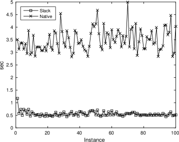
Figure 1: Cor vs. Cor-Slack. Instance-by-instance running times for $m=20$.

7.3 The closest correlation matrix problem — extended version

We consider an extended formulation for Cor as suggested in one of PENLAB’s examples, with extra constraints to bound the eigenvalues of the matrices:

$$\begin{array}[]{ll}\underset{X,z}{\mbox{minimize }}&\langle zX-H,zX-H\rangle\\ \mbox{subject to }&zX_{ii}=1\qquad\forall\,i,\\ &I_{m}\preceq X\preceq\kappa I_{m},\end{array}$$ (Cor-Ext)

where $\kappa$ is some positive number greater than $1$ and the notation $X\succeq\kappa I_{m}$ means $X-\kappa I_{m}\in{\mathcal{S}^{m}_{+}}$. This is a nonconvex problem, and using slack variables, we obtain the following formulation:

$$\begin{array}[]{l}\begin{array}[]{ll}\underset{X,Y_{1},Y_{2},z}{\mbox{minimize }}&\langle zX-H,zX-H\rangle\\ \end{array}\\ \begin{array}[]{llll}\mbox{subject to }&zX_{ii}&=1&\forall\,i,\\ &\kappa I_{m}-X&={Y_{1}\circ Y_{1}},&\\ &X-I_{m}&={Y_{2}\circ Y_{2}}.&\end{array}\end{array}$$ (Cor-Ext-Slack)

In our experiments, we set $\kappa=10$. As before, we generated 100 symmetric matrices $H$ whose diagonal elements are all $1$ and other elements are uniform random numbers between $-1$ and $1$. For Cor-Ext, we used $z=1$ and $X=I_{m}$ as initial points. For Cor-Ext-Slack, we used an infeasible starting point $z=1$, $X=Y_{2}=I_{m}$ and $Y_{1}=3I_{m}$. We solved problems with $m=5,10,15,20$ and the results can be found in Table 3. The columns have the same meaning as in Section7.2. This time, we saw a higher failure rate for the formulation Cor-Ext-Slack. We tried a few different initial points, but the results stayed mostly the same. The best results were obtained for the case $m=5$ and $m=10$, where Cor-Ext-Slack had a performance comparable to Cor-Ext, although the latter seldom failed. For $m=15$ and $m=20$, Cor-Ext-Slack was slower than Cor-Ext, which is expected, because the number of variables increased significantly. However, it was still able to solve the majority of instances. In Figure 2, we show the comparison of running times, instance-by-instance, for the cases $m=10$ and $m=20$.

Table 3: Comparison between Cor-Ext and Cor-Ext-Slack

	Cor-Ext-Slack				Cor-Ext
$m$	mean (s)	min (s)	max (s)	fail	mean (s)	min (s)	max (s)	fail
5	0.236	0.130	0.830	15	0.445	0.250	2.130	1
10	0.741	0.420	2.580	3	1.206	0.580	7.300	0
15	4.651	2.090	26.96	15	3.809	1.960	14.12	0
20	24.32	15.20	69.34	8	9.288	5.150	36.81	0

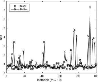
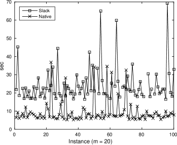
Figure 2: Cor-Ext vs Cor-Ext-Slack. Instance-by-instance running times for $m=10$ and $m=20$. Failures are represented by omitting the corresponding running time.

8 Final remarks

In this article, we have shown that the optimality conditions for (P1) and (P2) are essentially the same. One intriguing part of this connection is the fact that the addition of squared slack variables seems to be enough to capture a great deal of the structure of ${\mathcal{S}^{m}_{+}}$. The natural progression from here is to expand the results to symmetric cones. In this article, we already saw some results that have a distinct Jordan-algebraic flavor, such as Lemma 2.1. It would be interesting to see how these results can be further extended and, whether clean proofs can be obtained without recoursing to the classification of simple Euclidean Jordan algebras.

As for the computational results, we found it mildly surprising that the slack variables approach was able to outperform the “native” approach in many instances. This warrants a deeper investigation of whether this could be a reliable tool for attacking NSDPs that are not linear. These are precisely the ones that are not covered by the earlier work by Burer and Monteiro [5, 6].

References

- [1] Barvinok, A.: Problems of distance geometry and convex properties of quadratic maps. Discrete Comput. Geom. 13(1), 189–202 (1995)
- [2] Bernstein, D.S.: Matrix Mathematics: Theory, Facts, and Formulas, 2nd edn. Princeton University Press (2009)
- [3] Bertsekas, D.P.: Nonlinear Programming, 2nd edn. Athena Scientific (1999)
- [4] Bonnans, J.F., Cominetti, R., Shapiro, A.: Second order optimality conditions based on parabolic second order tangent sets. SIAM J. Optim. 9(2), 466–492 (1999)
- [5] Burer, S., Monteiro, R.D.: A nonlinear programming algorithm for solving semidefinite programs via low-rank factorization. Math. Program. 95(2), 329–357 (2003)
- [6] Burer, S., Monteiro, R.D.: Local minima and convergence in low-rank semidefinite programming. Math. Program. 103(3), 427–444 (2005)
- [7] Cominetti, R.: Metric regularity, tangent sets, and second-order optimality conditions. Appl. Math. Optim. 21(1), 265–287 (1990)
- [8] Fiala, J., Kočvara, M., Stingl, M.: PENLAB: A matlab solver for nonlinear semidefinite optimization. ArXiv e-prints (2013)
- [9] Forsgren, A.: Optimality conditions for nonconvex semidefinite programming. Math. Program. 88(1), 105–128 (2000)
- [10] Fukuda, E.H., Fukushima, M.: The use of squared slack variables in nonlinear second-order cone programming. Submitted (2015)
- [11] Hock, W., Schittkowski, K.: Test examples for nonlinear programming codes. J. Optim. Theory Appl. 30(1), 127–129 (1980)
- [12] Jarre, F.: Elementary optimality conditions for nonlinear SDPs. In: Handbook on Semidefinite, Conic and Polynomial Optimization, International Series in Operations Research & Management Science, vol. 166, pp. 455–470. Springer (2012)
- [13] Kawasaki, H.: An envelope-like effect of infinitely many inequality constraints on second-order necessary conditions for minimization problems. Math. Program. 41(1-3), 73–96 (1988)
- [14] Kočvara, M., Stingl, M.: PENNON: A code for convex nonlinear and semidefinite programming. Optim. Methods Softw. 18(3), 317–333 (2003)
- [15] Nocedal, J., Wright, S.J.: Numerical Optimization, 1st edn. Springer Verlag, New York (1999)
- [16] Pataki, G.: On the rank of extreme matrices in semidefinite programs and the multiplicity of optimal eigenvalues. Math. Oper. Res. 23(2), 339–358 (1998)
- [17] Pataki, G.: The geometry of semidefinite programming. In: H. Wolkowicz, R. Saigal, L. Vandenberghe (eds.) Handbook of Semidefinite Programming: Theory, Algorithms, and Applications. Kluwer Academic Publishers (2000)
- [18] Robinson, S.M.: Stability theory for systems of inequalities, part II: Differentiable nonlinear systems. SIAM J. Numer. Anal. 13(4), 497–513 (1976)
- [19] Schittkowski, K.: Test examples for nonlinear programming codes – all problems from the Hock-Schittkowski-collection. Tech. rep., Department of Computer Science, University of Bayreuth (2009)
- [20] Shapiro, A.: First and second order analysis of nonlinear semidefinite programs. Math. Program. 77(1), 301–320 (1997)
- [21] Sturm, J.F.: Similarity and other spectral relations for symmetric cones. Linear Algebra Appl. 312(1-3), 135–154 (2000)
- [22] Yamashita, H., Yabe, H.: A survey of numerical methods for nonlinear semidefinite programming. J. Oper. Res. Soc. Jpn. 58(1), 24–60 (2015)