Three Twin Neutrinos: Evidence from LSND and MiniBooNE
Abstract
We construct a neutrino model of three twin neutrinos in light of the neutrino appearance excesses at LSND and MiniBooNE. The model, which includes a twin parity, naturally predicts identical lepton Yukawa structures in the Standard Model and the twin sectors. As a result, a universal mixing angle controls all three twin neutrino couplings to the Standard Model charged leptons. This mixing angle is predicted to be the ratio of the electroweak scale over the composite scale of the Higgs boson and has the right order of magnitude to fit the data. The heavy twin neutrinos decay within the experimental lengths into active neutrinos plus a long-lived Majoron and can provide a good fit, at around confidence level, to the LSND and MiniBooNE appearance data while simultaneously satisfying the disappearance constraints. For the Majorana neutrino case, the fact that neutrinos have a larger scattering cross section than anti-neutrinos provides a natural explanation for MiniBooNE’s observation of a larger anti-neutrino appearance excess.
I Introduction
The past decade has seen a series of anomalies emerge in short baseline (SBL) neutrino oscillation experiments which cannot be explained within the three active neutrino framework of the Standard Model (SM). Here, SBL refers to experiments with the ratio of the oscillation distance over the neutrino energy, , which are sensitive to neutrino oscillations involving mass squared splittings . The LSND experiment Aguilar:2001ty reports evidence of oscillation consistent with , as well as a less dramatic excess for oscillation Athanassopoulos:1997er . The MiniBooNE collaboration also searched for the same signal, reporting excesses in both electron and anti-electron neutrino events Aguilar-Arevalo:2013pmq , again suggesting oscillations of the form and , consistent with the LSND results. Together, these observations lead to the tantalizing suggestion of additional “sterile” neutrino flavors at a mass scale of .
Many schemes have been considered to fit the excess, including 3 active plus sterile neutrino oscillation schemes (3+), with most of the attention being focused on and Conrad:2013mka ; Karagiorgi:2006jf ; Giunti:2010jt ; Nelson:2010hz ; Kopp:2011qd ; Fan:2012ca ; Kuflik:2012sw ; Huang:2013zga ; Aguilar-Arevalo:2013pmq ; Kopp:2013vaa . While even the simple 3+1 scheme can provide a good fit to the () appearance excesses, these fits are in tension with , and disappearance constraints from MiniBooNE+SciBooNE Cheng:2012yy ; Mahn:2011ea and LSND+KARMEN Conrad:2011ce , respectively. To ameliorate the disappearance constraint, some authors have also considered fairly prompt decay of sterile neutrinos PalomaresRuiz:2005vf (i.e. ) to allow the decay of sterile neutrinos to active neutrinos within the experimental lengths. In most cases, a decay of this form requires the coupling of neutrinos to a new light state (potentially a Majoron Chikashige:1980qk ; Chikashige:1980ui ; Gelmini:1980re ), which enables the sterile neutrinos to decay through the process . While some authors have also considered decays of the form Gninenko:2009ks to explain the MiniBooNE signal, this decay cannot explain the LSND excess and we will not consider it here.
Very little attention has been focused on the 3+3 oscillation scheme, mainly in the interest of minimality and because there was no clear indication that adding a third sterile neutrino would improve the 3+2 fit. However, when the sterile neutrino sector is embedded within a model that “mirrors” the SM particle content Kobzarev:1966qya ; Berezhiani:1995yi ; FOOT199167 , the 3+3 scenario becomes natural to consider. One well motivated model of this type is the “Twin Higgs” model Chacko:2005pe ; Craig:2015pha , although others have been considered Barbieri:2005ri ; Foot200775 ; Foot:1999ph ; DELAGUILA1985237 ; Foot:1996hp . The Twin Higgs model contains a full or partial copy of the SM gauge group and particle content, with couplings in the two sectors related by a discrete symmetry. The particle content in each sector, usually denoted and , transforms under its own gauge group and is sterile with respect to the other sector. An attractive feature of the Twin Higgs model is that it provides a solution to the little hierarchy problem without requiring new particles charged under the SM gauge group, at least below the cutoff of the effective theory. In this model, the Higgs field is a pseudo-Nambu Goldstone boson (PNGB) associated with spontaneous breaking of an approximate global symmetry. A twin symmetry is introduced to constrain the form of corrections to the PNGB Higgs potential, allowing natural electroweak symmetry breaking with no quadratically divergent corrections to the Higgs mass at one-loop level.
In this paper, we construct a 3+3 neutrino model within the Twin Higgs framework, although many of our phenomenological studies can be applied to other models with similar flavor structures. Two higher dimensional operators turn out to be relevant for the neutrino sectors. The first operator is dimension-five and respects both the and symmetries. After the Higgs fields develop their vacuum expectation values (VEV’s), three out of the total six neutrinos become massive and can be identified as the three sterile neutrinos. Because of -enforced Yukawa alignment between the two sectors, only one universal mixing angle in addition to the usual Pontecorvo-Maki-Nakagawa-Sakata (PMNS) matrix is required to describe how the three sterile neutrinos interact with the SM charged leptons. This mixing angle is predicted to be the ratio of two Higgs VEV’s, , and has the right order of magnitude to fit the SBL excesses. The second relevant operator is dimension-six, which is -conserving and -breaking. It is responsible for coupling the Majoron to neutrinos and additionally for providing mass to the light active neutrinos. We will show that after satisfying various constraints, the three heavy sterile neutrinos can decay into active neutrinos plus one Majoron with the decay distance within the experimental lengths. In what follows, we will analyze oscillation and decay of Dirac and Majorana sterile neutrinos within the context of this 3+3 “Twin Neutrino” model. We will show that promptly decaying sterile neutrinos in this model can provide a good fit to the LSND and MiniBooNE anomalies.
II The Twin Neutrino Model
Motivated by the Twin Higgs model, we consider a global non-Abelian symmetry in the electroweak parts of both the SM and twin sectors. The two Higgs doublets and , which transform under and gauge symmetries, can be grouped together as a quadruplet of : . At the minimum of its invariant potential, the quadruplet develops a VEV of , spontaneously breaking down to its subgroup. As a result, there are seven Nambu-Goldstone-bosons (NGB’s) in the low energy theory below the cutoff . Turning on electroweak gauge interactions in both sectors, the quadruplet VEV breaks the twin electroweak gauge symmetry to a single with three NGB’s eaten by the three massive gauge bosons and . 111An additional Higgs mechanism may be required to provide the twin photon mass. The remaining four NGB’s can be identified as the SM Higgs doublet, , which acquire mass and become PNGB’s after turning on breaking gauge or Yukawa interactions.
The little hierarchy problem can be alleviated by imposing an additional symmetry between the two sectors which forces all couplings to be the same. This is because in the gauge sector, the one loop corrections to the Higgs mass which are quadratic in have the form and are independent of the PNGB Higgs field. In addition, the logarithmically divergent part contributes to the coefficient of the -breaking operator at the order of , so the Higgs field mass is generically suppressed compared to the VEV TeV. To obtain the lighter Higgs boson mass at 125 GeV, the coefficient is needed to be around 1/4, which suggests additional breaking terms in the scalar potential. Minimizing the potential for the two Higgs doublets with small -breaking terms, the ratio of the two VEV’s is
| (1) |
with the electroweak VEV, GeV. Later we will show that this ratio will be crucial to determine the fermion mass spectrum in the twin sector.
The fermion Yukawa couplings explicitly break the global ) symmetry. The twin parity is required to ensure that there are no corrections to the SM Higgs mass proportional to at the one-loop level. Therefore, we keep the Yukawa couplings in both sectors to be exactly the same, both for charged leptons and neutrinos. For the charged leptons, the -invariant and -breaking Yukawa couplings in the Lagrangian are
| (2) |
Here, the indexes “” denote lepton flavors. After inputting the scalar VEV’s, we have the three twin charged-lepton masses exactly proportional to the SM ones: . For instance, the twin electron is anticipated to have a mass of .
II.1 Majorana Neutrinos
In the neutrino sector, we will consider both Majorana and Dirac neutrino cases and will only focus on the spectrum with normal ordering, which is preferred for the Majorana case. In this subsection, we first study the Majorana neutrinos for both SM and twin sectors. Different from the charged-lepton sector, we can have the following -invariant and -conserving Majorana mass operators
| (3) |
Here, and with . The cutoff, , could be related to the some heavy right-handed neutrino masses to realize the See-Saw mechanism. After Higgs doublets get their VEV’s, the linear combinations are massive and are approximately the three sterile neutrino states. To provide mass for other combinations, we introduce the following -invariant and -breaking dimension-six operator
| (4) |
Here, the new gauge-singlet scalar carries both SM and twin lepton numbers. Furthermore, one could define a discrete symmetry in the twin sector with , and , such that additional operators for coupling to only SM leptons are forbidden. This discrete symmetry is important for our later discussion of -related phenomenology. The Yukawa couplings are chosen to be identical for Eq. (3) and Eq. (4), which could originate from a UV theory at a much higher than TeV scale.
After develops a VEV with , 222We take the VEV of to be a real number. Its complex phase is physical, but will not change our phenomenological study later. the neutrino mass matrix is
| (7) | |||||
| (8) |
In the leading order of and , the three heavy (sterile) neutrino masses are
| (9) |
where is the eigenvalue of the Yukawa matrix . Because of flavor alignment in the SM and twin sectors, the ratios of the neutrino masses satisfy
| (10) |
to the leading order of the small parameter, , in our model. For a normal ordering mass spectrum of active neutrinos, , and from Ref. Agashe:2014kda , we have eV2 and eV2. The twin neutrino masses are shown in Fig. 1 for two different values of .
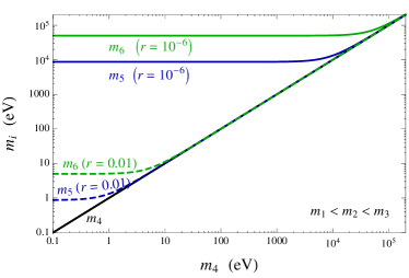
In the charged-lepton mass-eigenstate basis, the diagonalization unitary matrix can be written in terms of a tensor product
| (11) |
where is the PMNS matrix in the SM (the experimental values are taken from Ref. Agashe:2014kda ) and is a rotation matrix
| (14) |
To the leading order of , the new mixing angle between the SM and twin neutrino sectors is
| (15) |
Consequently, the three active neutrinos () interact with the SM charged leptons with a strength proportional to , while the three sterile neutrinos () have interactions suppressed by . The sterile neutrino interaction strengths with SM charged leptons are therefore related to the fine-tuning problem for the SM Higgs boson.
In this model, there is a PNGB or Majoron Chikashige:1980qk ; Chikashige:1980ui ; Gelmini:1980re associated with the global symmetry breaking of . The relevant Yukawa couplings for the Majoron particle, , defined as , in our models is flavor diagonal and are
| (16) |
The sterile neutrinos are not stable particles and have the decay widths of
| (17) | |||||
In our numerical study later, we will focus on the parameter region of or and .
Since the mass operators in Eq. (3) explicitly break the symmetry, we anticipate a non-zero mass for the Majoron filed, . The one-loop diagram mediated by and generates a mass for
| (18) | |||||
For a normal ordering neutrino mass spectrum, we have eV for keV, and . The Majoron decay width is
| (19) |
For a normal ordering neutrino mass spectrum, eV, and , the decay width at rest is eV.
II.2 Dirac Neutrinos
For the Dirac neutrino case, one need to introduce an additional set of right-handed neutrinos in both the SM and twin sectors. The -invariant and -conserving Dirac mass operators are
| (20) |
Furthermore, the following and -breaking dimension-five operator is introduced to provide light neutrino masses and decay couplings for the heavy neutrinos
| (21) |
After develops a VEV with , the neutrino mass matrix is
| (24) | |||||
| (25) |
with the left-handed rotation matrix as
| (26) |
Using the same parametrization in Eq. (15) and in the limit of , we still have . The mass ratios for this Dirac neutrino model is
| (27) |
In the Dirac neutrino model, we also have a PNGB associated with the symmetry breaking of . The couplings of the Majoron, , parametrized by are
| (28) | |||||
| (29) |
The sterile neutrino decay widths are
| (30) |
In our model, the active neutrinos from sterile neutrino decays are left-handed.
III Constraints from unitary, meson decays and neutrinoless double beta decay
For both the Majorana and Dirac neutrino models, we have the model parameters: , (related to the coupling ), and . In this section, we study the existing constraints on our model parameters from unitarity of the active neutrino mixing matrix, neutrinoless double beta decay and meson decays.
The mixing between active and twin neutrinos reduces the couplings of active neutrinos to charged leptons in the SM. The mixing matrix, , is a unitary matrix in our model, but the mixing matrix, , is not unitary and has the normalization property of . Using the results in Ref. Parke:2015goa and neglecting the effects of sterile decay products, we have found that
| (31) |
at C.L.
There are additional bounds on the sterile neutrino decay widths from the pion and kaon three-body decay into the new Majoron state and the electron-muon universality tests of their total leptonic widths (see Ref. deGouvea:2015euy for a recent summary). Using the analysis in Ref. Barger:1981vd and the measurement of branching ratio Britton:1993cj ; Aguilar-Arevalo:2015cdf , the predicted deviation from universality is with the experimental value of (the updated value of provides a similar bound), so the bound on our model parameters is
| (32) |
at 90% C.L. Here, for the Majorana(Dirac) neutrino case. In Fig. 2, we show the constraints on our model parameters in the and plane.
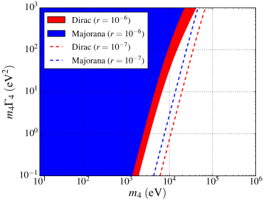
For the Majorana neutrino case, searches for the neutrinoless double beta decay can also impose bounds on our model parameter space. The amplitude of is proportional to the effective Majorana mass
| (33) |
The -violating phases can affect the predicted effective Majorana mass. In our model, we have identical Majorana and Dirac phases for the SM and twin sectors. In Fig. 3, we show the allowed parameter space by allowing arbitrary Majorana phases but fixed Dirac phase of .
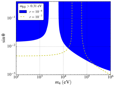
We did not find additional processes like or provide more stringent bounds than from and meson decays.
Because of the fairly large interaction strength () among sterile neutrinos, active neutrinos and the Majoron particle, both sterile neutrinos and the Majoron particles stay within the supernova core. Our model does not have an additional energy loss problem for supernova SN1987A. For sterile neutrinos with a mass below around 1 MeV, they contribute to additional relativistic degrees of freedom and are constrained from BBN Barger:2003zg ; Ade:2015xua . However, to have a conclusive statement, additional analysis or non-standard cosmology should be taken into account. We do not explore these directions here.
IV Neutrino Appearance and Disappearance
In this section, we write down general neutrino appearance and disappearance formulas for our model. Since we have both oscillation and decay, we will keep both effects for neutrino appearance and disappearance. For the short-baseline experiments, the differential probability for a neutrino of flavor with energy converting into a neutrino of flavor with energy in the interval of is Lindner:2001fx ; PalomaresRuiz:2005vf
| (34) | |||||
Here, the neutrino decay widths, for and for , are defined in the rest frame. for the Majorana(Dirac) neutrino case. For the case of neutrino goes to neutrino, the energy spectrum function is . For the Majorana model, the helicity-flip formula for has only the second term (the decaying part) with a different energy spectrum function, . For the case with initial anti-neutrinos, one should replace the elements of by their complex conjugates.
In our numerical studies, we will focus on the pure oscillation case as well as the case where the decay effect dominates. For the pure oscillation case with and in the limits of and (the short-baseline approximation), the neutrino appearance probability is
| (35) | |||||
for . Here, the phase . The formula for the anti-neutrino case can be obtained by a replacement of . In our model, only a single Dirac phase enters both sectors. In the small mixing angle limit of and order of unity, we have , . So, a large -violating phase can affect the (anti-)neutrino appearance probabilities. The disappearance probability is independent of -violating phase and has
| (36) |
Comparing Eqs. (35) and (36), one can see that the appearance probability is suppressed by , while the disappearance is only suppressed by . We will later show because of this fact it is challenging to only use oscillation to explain LSND and MiniBooNE anomalies.
For the case in which sterile neutrino decay effects are dominant and in the limit of , the appearance probability is
| (37) | |||||
For the Majorana model, the helicity-flip formula for is similar but using . The disappearance has contributions from both terms in Eq. (34) and is
| (38) | |||||
ignoring additional terms suppressed by . One can see that for the decay case both appearance and disappearance are suppressed by the same power of . This fact will make the decay model a better fit to LSND and MiniBooNE data.
V Fit to LSND, MiniBooNE and SciBooNE data
In this section, we will consider both cases for interpreting short-baseline experimental data with or without sterile neutrino decays. For the first case without sterile neutrino decays, the energy spectrum of the neutrinos near the far detector follows the initial injected neutrino spectrum. On the other hand, for the second case with sterile neutrino decays, additional care should be taken to account for the energy spectrum change.
V.1 Oscillation without decay
To interpret the LSND event excess of anti-neutrino appearance, Aguilar:2001ty (we will ignore the less significant excess in the neutrino appearance observed by LSND Athanassopoulos:1997er ), and to derive the preferred model parameter space, we follow Ref. Giunti:2010jt to account the energy spectrum as well as the conversion of the neutrino energy spectrum to measured positron energy spectrum, , from the inverse neutron decay process . The measured positron energy has the range of . For the simplest sterile neutrino model, we have reproduced the LSND contours in Ref. Giunti:2010jt .
For the MiniBooNE and appearance analysis based on initial anti-neutrino and neutrino fluxes Aguilar-Arevalo:2013pmq , we use the data released by MiniBooNe collaboration MiniBooNE to derive the preferred contours in our model parameter space. We combine the two data sets in the (anti-)neutrino energy range of . Again, for the simplest sterile neutrino model, we reproduce the contours in the MiniBooNE publication Aguilar-Arevalo:2013pmq .
For the constraints from (anti-)neutrino disappearance, we use the combined SciBooNE and MiniBooNE analysis Cheng:2012yy for the anti-neutrino disappearance measurement, which provides more stringent constraints than the ones from the neutrino disappearance measurement Mahn:2011ea . We use the publicly available data SciBooNE to constrain our model parameter space. We have also checked additional constraints from appearance searches by KARMEN Armbruster:2002mp but found them to be less stringent, and we will not report them here.
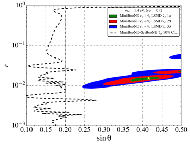
In Fig. 4, we show the LSND and MniBooNE preferred contours in terms of our model parameters: and by fixing eV and assuming , which provides a better fit than no violation with . From a three-dimensional parameter scan, we have found the point with the smallest at , and eV. This is an improvement by compared to the no oscillation fit. Unfortunately, the disappearance constraints from SciBooNE and MiniBooNE exclude all the appearance-data-preferred region. Furthermore, the constraints from unitarity of the three active neutrinos also exclude the LSND and MniBooNE preferred contours. This can be understood by the formulas in Section IV, which show that the appearance probabilities for the pure oscillation case have an additional with respect to the disappearance probabilities. The tension for appearance and disappearance data is a general feature even for a general global fit Kopp:2013vaa ; Giunti:2013aea .
V.2 Oscillation with decay
For the second case with the decay effects dominant, we need to know more information about the detectors. The first important piece of information is to know whether the sterile neutrinos generated at the source location have already decayed or not. It can be seen from Eq. (37) that in order to have a larger appearance probability, it is preferable to have all sterile neutrinos decay within the experimental lengths. Taking the Lorentz boost into account, this means . LSND has the distance range of m and the energy range of MeV; MiniBooNE has the distance around 540 m and the energy range of MeV; SciBooNE has the distance around 100 m and the energy range of MeV for the disappearance analysis Cheng:2012yy . Altogether, if eV2, the majority of sterile neutrinos have already decayed before reaching the detector. We also note that for large values of , all sterile neutrinos decay promptly and only and are relevant parameters for both appearance and disappearance experiments.
Both LSND and MiniBooNE are able to generate or initial fluxes. On the other hand, for the appeared electron neutrino or anti-neutrinos in the detectors, the LSND detectors are different from MiniBooNE and SciBooNE. The LSND experiment can distinguish and because after interacts via inverse beta decay in the mineral oil target of LSND, both a prompt positron and a correlated 2.2 MeV photon from neutron capture appear. This twofold signature is not true for . On the other hand, the MiniBooNE and SciBooNE can not distinguish and . In order to compare to the MiniBooNE and SciBooNE data, we need to add both and . Furthermore, we also note that the quasi-elastic cross sections for and interacting with CH2 in MiniBooNE are different. Using the cross sections in GENIE Andreopoulos:2015wxa and for the relevant energy range of MeV at MiniBooNE, we have
| (39) |
which is mainly due to from a negative axial-vector form factor Formaggio:2013kya . We will show later that because of different scattering cross sections the Majorana and Dirac models have different features for fitting appearance data.
Before we present our results, we also want to comment on the fact that the LSND or the MiniBooNE measured neutrino transition probability is not simply Eq. (34) for the sterile neutrino decay case. They have the measured probability for each energy bin to be Aguilar-Arevalo:2014xrr . For the full oscillation model, their measured probability matches to the theoretical oscillation probability. For the decay case at hand, the energy spectra of the initial neutrino flux at the source and the final flux at the detector are different. To compare to the LSND and MiniBooNE data plots, we use the following probability
| (40) | |||||
Here, the symbol “” means function convolution. For the Majorana model, we have for LSND and for MiniBooNE. For the Dirac model, we have for both LSND and MiniBooNE. For the initial anti-neutrino experiments, one just makes the interchange of . In deriving the above equation, we have also made the quasi-elastic approximation with the outgoing electron(positron) energy equal to the incoming neutrino(anti-neutrino) energy.
Based on Eqs. (39)(40), there is an interesting observation about our Majorana model prediction for MiniBooNE. Under the approximation of the same energy spectra of the initial fluxes, , one has
| (41) |
simply from the fact that the neutrino quasi-elastic cross section is larger than the anti-neutrino one.
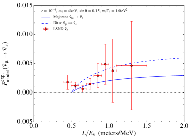
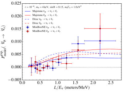
In Fig. 5, we show a comparison of a benchmark model point with , keV, and eV2, to the LSND data. The Dirac model has probabilities higher than the Majorana model simply by a factor of two. Note that the starting points of the model curves are higher than the actual data starting point. This is due to the approximation of using the shortest distance m and the maximal neutrino energy of MeV from muon decays at rest Giunti:2010jt . Similarly for MiniBooNE, in Fig. 6 we show both Majorana and Dirac model predictions for the same benchmark model point. As we argued before, the Majorana model has a larger excess for the initial run than the initial run at MiniBooNE. For the Dirac model, there is also some difference between the initial and runs, which comes from the slightly different energy spectra for the initial fluxes.
In Fig. 7 and for the Majorana model, we show the contour plot for the two most relevant model parameters, and , to fit the MiniBooNE and LSND appearance data. Also shown in this plot is the 90% C.L. constraints from MiniBooNE plus SciBooNE. Different from the pure oscillation case in Fig. 4, the constraint from the disappearance data is not stringent enough to rule out the best fit region for appearance data. For and keV (allowed from the neutrinoless double beta decay constraints in Fig. 3), the smallest to fit both MiniBooNE (using their Monte Carlo samples) and LSND (using their energy resolution) has and eV2. Compared to the fit without new physics, the difference is . For two degrees of freedom this means that the background-only fit has a -probability of (or ) relative to our twin neutrino decay model.
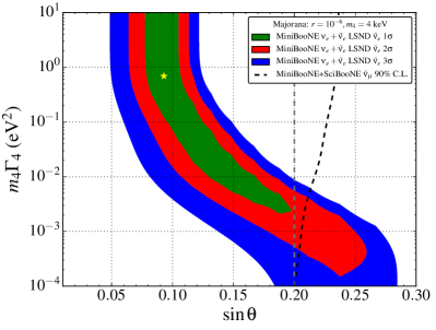
For the best fit point of the Majorana neutrino model, the six neutrino masses are 0.004 eV, 0.0096 eV, 0.050 eV, 4 keV, 9.56 keV, 50.0 keV. The three sterile neutrino widths are eV, eV and eV. The decay Yukawa coupling defined in Eq. (16) is . As a result, the Majoron receives a loop-generated contribution to its mass with a value of around 3 eV, which means that the Majoron can decay into all three active neutrinos. For the typical neutrino energy of 30 MeV at LSND (500 MeV at MiniBooNE), the Majoron travels far enough that it can be treated as an invisible particle for both experiments.
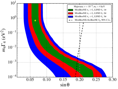
For the Dirac neutrino case, we show the allowed parameter region in Fig. 8 for fixed values of and keV. The best fit point is at and eV2 with (a probability of or ) compared to the fit without the three twin neutrinos. The Dirac model provides a slightly worse fit than the Majorana model, because the Majorana model has a higher model prediction for the anti-neutrino appearance probability than the neutrino one. We also note that the anti-neutrino disappearance constraint from MiniBooNE plus SciBooNE for the Dirac model is more stringent than for the Majorana model. This is simply due to the larger scattering cross section of neutrinos than anti-neutrinos.
VI Discussion and Conclusions
The twin neutrino scenario is very predictive. The neutrino mixing matrix is fixed by the usual PMNS matrix and the ratio of the Higgs VEV’s in the two sectors. Additionally, the signals observed by LSND and MiniBooNE dictates either or to be around . In the Majorana sterile neutrino decay scenario, the model also requires a normal ordering mass spectrum for the three active neutrinos to avoid the decay constraint. Because the SM and twin sectors are closely related by the twin symmetry, the number of free parameters is greatly reduced. The next generation neutrino experiments probing the twin sector neutrinos can also provide information about the SM active neutrino sector. Combining the experimental information from both sectors, it is very likely that we can completely determine all the parameters in the neutrino sector.
The decay sterile neutrino scenario provides a novel explanation to the LSND and MiniBooNE anomalies. Depending on whether neutrinos are Dirac or Majorana, one could have either only or both and to be decay products of the twin neutrino components in . For the Majorana case, the MiniBooNE run can have a larger excess than the run. This is because as a product of the twin partner has a larger scattering cross section than . Our explanation for the larger run excess does not require violation, which is necessary for the pure oscillation explanation.
Future experiments like MicroBooNE Soderberg:2009rz (see also Ref. Dutta:2015nlo for other interesting proposals) may provide decisive tests for the LSND and MiniBooNE excesses. Their results will not just cover our twin neutrino decay scenario, but also the pure oscillation interpretation. We also note that the IceCube collaboration is finalizing their (eV) sterile neutrino searches. Some preliminary results have shown significant improvement on constraining oscillation parameters Carlos:2015 ; Jones:2015bya . The IceCube bound is based on oscillation effects with a dramatical enhancement of the oscillation amplitude due to matter effects at TeV energies. Although our twin neutrino decay scenario is unlikely to be constrained by the IceCube search, it is interesting to explore how to search for the three twin neutrinos at large cosmic-ray neutrino experiments.
In summary, motivated by the LSND and MiniBooNE excesses, we have constructed an interesting neutrino model to link the sterile neutrino phenomenology to the new TeV-scale physics associated with electroweak symmetry breaking.
Acknowledgments. We would like to thank Vernon Barger, Josh Berger and Lisa Everett for useful discussion and comments. This work is supported by the U. S. Department of Energy under the contract DE-FG-02-95ER40896. Jordi Salvado is also supported by FPA2011-29678 and FPA2014-57816-P.
References
- (1) LSND Collaboration, A. Aguilar-Arevalo et al., Evidence for neutrino oscillations from the observation of anti-neutrino(electron) appearance in a anti-neutrino(muon) beam, Phys. Rev. D64 (2001) 112007, [hep-ex/0104049].
- (2) LSND Collaboration, C. Athanassopoulos et al., Evidence for muon-neutrino electron-neutrino oscillations from pion decay in flight neutrinos, Phys. Rev. C58 (1998) 2489–2511, [nucl-ex/9706006].
- (3) MiniBooNE Collaboration, A. A. Aguilar-Arevalo et al., Improved Search for Oscillations in the MiniBooNE Experiment, Phys. Rev. Lett. 110 (2013) 161801, [arXiv:1207.4809].
- (4) J. M. Conrad, W. C. Louis, and M. H. Shaevitz, The LSND and MiniBooNE Oscillation Searches at High , Ann. Rev. Nucl. Part. Sci. 63 (2013) 45–67, [arXiv:1306.6494].
- (5) G. Karagiorgi, A. Aguilar-Arevalo, J. M. Conrad, M. H. Shaevitz, K. Whisnant, M. Sorel, and V. Barger, Leptonic CP violation studies at MiniBooNE in the (3+2) sterile neutrino oscillation hypothesis, Phys. Rev. D75 (2007) 013011, [hep-ph/0609177]. [Erratum: Phys. Rev.D80,099902(2009)].
- (6) C. Giunti and M. Laveder, Short-Baseline Oscillations, Phys. Rev. D82 (2010) 093016, [arXiv:1010.1395].
- (7) A. E. Nelson, Effects of CP Violation from Neutral Heavy Fermions on Neutrino Oscillations, and the LSND/MiniBooNE Anomalies, Phys. Rev. D84 (2011) 053001, [arXiv:1010.3970].
- (8) J. Kopp, M. Maltoni, and T. Schwetz, Are there sterile neutrinos at the eV scale?, Phys. Rev. Lett. 107 (2011) 091801, [arXiv:1103.4570].
- (9) J. Fan and P. Langacker, Light Sterile Neutrinos and Short Baseline Neutrino Oscillation Anomalies, JHEP 04 (2012) 083, [arXiv:1201.6662].
- (10) E. Kuflik, S. D. McDermott, and K. M. Zurek, Neutrino Phenomenology in a 3+1+1 Framework, Phys. Rev. D86 (2012) 033015, [arXiv:1205.1791].
- (11) J. Huang and A. E. Nelson, MeV dark matter in the 3+1+1 model, Phys. Rev. D88 (2013) 033016, [arXiv:1306.6079].
- (12) J. Kopp, P. A. N. Machado, M. Maltoni, and T. Schwetz, Sterile Neutrino Oscillations: The Global Picture, JHEP 05 (2013) 050, [arXiv:1303.3011].
- (13) SciBooNE, MiniBooNE Collaboration, G. Cheng et al., Dual baseline search for muon antineutrino disappearance at , Phys. Rev. D86 (2012) 052009, [arXiv:1208.0322].
- (14) SciBooNE, MiniBooNE Collaboration, K. B. M. Mahn et al., Dual baseline search for muon neutrino disappearance at , Phys. Rev. D85 (2012) 032007, [arXiv:1106.5685].
- (15) J. M. Conrad and M. H. Shaevitz, Limits on Electron Neutrino Disappearance from the KARMEN and LSND - Carbon Cross Section Data, Phys. Rev. D85 (2012) 013017, [arXiv:1106.5552].
- (16) S. Palomares-Ruiz, S. Pascoli, and T. Schwetz, Explaining LSND by a decaying sterile neutrino, JHEP 09 (2005) 048, [hep-ph/0505216].
- (17) Y. Chikashige, R. N. Mohapatra, and R. D. Peccei, Spontaneously Broken Lepton Number and Cosmological Constraints on the Neutrino Mass Spectrum, Phys. Rev. Lett. 45 (1980) 1926.
- (18) Y. Chikashige, R. N. Mohapatra, and R. D. Peccei, Are There Real Goldstone Bosons Associated with Broken Lepton Number?, Phys. Lett. B98 (1981) 265.
- (19) G. B. Gelmini and M. Roncadelli, Left-Handed Neutrino Mass Scale and Spontaneously Broken Lepton Number, Phys. Lett. B99 (1981) 411.
- (20) S. N. Gninenko, The MiniBooNE anomaly and heavy neutrino decay, Phys. Rev. Lett. 103 (2009) 241802, [arXiv:0902.3802].
- (21) I. Yu. Kobzarev, L. B. Okun, and I. Ya. Pomeranchuk, On the possibility of experimental observation of mirror particles, Sov. J. Nucl. Phys. 3 (1966), no. 6 837–841. [Yad. Fiz.3,1154(1966)].
- (22) Z. G. Berezhiani and R. N. Mohapatra, Reconciling present neutrino puzzles: Sterile neutrinos as mirror neutrinos, Phys. Rev. D52 (1995) 6607–6611, [hep-ph/9505385].
- (23) R. Foot, H. Lew, and R. Volkas, A model with fundamental improper spacetime symmetries, Physics Letters B 272 (1991), no. 1 67 – 70.
- (24) Z. Chacko, H.-S. Goh, and R. Harnik, The Twin Higgs: Natural electroweak breaking from mirror symmetry, Phys. Rev. Lett. 96 (2006) 231802, [hep-ph/0506256].
- (25) N. Craig, A. Katz, M. Strassler, and R. Sundrum, Naturalness in the Dark at the LHC, JHEP 07 (2015) 105, [arXiv:1501.05310].
- (26) R. Barbieri, T. Gregoire, and L. J. Hall, Mirror world at the large hadron collider, hep-ph/0509242.
- (27) R. Foot and R. R. Volkas, Natural electroweak symmetry breaking in generalised mirror matter models, Physics Letters B 645 (2007), no. 1 75 – 81.
- (28) R. Foot and R. R. Volkas, Implications of mirror neutrinos for early universe cosmology, Phys. Rev. D61 (2000) 043507, [hep-ph/9904336].
- (29) F. del Aguila, The standard model with mirror fermions, Annals of Physics 165 (1985), no. 1 237 – 258.
- (30) R. Foot and R. R. Volkas, The Exact parity symmetric model and big bang nucleosynthesis, Astropart. Phys. 7 (1997) 283–295, [hep-ph/9612245].
- (31) Particle Data Group Collaboration, K. A. Olive et al., Review of Particle Physics, Chin. Phys. C38 (2014) 090001. http://pdg.lbl.gov/2015/reviews/rpp2014-rev-neutrino-mixing.pdf.
- (32) S. Parke and M. Ross-Lonergan, Unitarity and the Three Flavour Neutrino Mixing Matrix, arXiv:1508.05095.
- (33) A. de Gouvê and A. Kobach, Global Constraints on a Heavy Neutrino, arXiv:1511.00683.
- (34) V. D. Barger, W.-Y. Keung, and S. Pakvasa, Majoron Emission by Neutrinos, Phys. Rev. D25 (1982) 907.
- (35) D. I. Britton et al., Measurement of the neutrino branching ratio, Phys. Rev. D49 (1994) 28–39.
- (36) PiENu Collaboration, A. Aguilar-Arevalo et al., Improved Measurement of the Branching Ratio, Phys. Rev. Lett. 115 (2015), no. 7 071801, [arXiv:1506.05845].
- (37) P. Guzowski, L. Barnes, J. Evans, G. Karagiorgi, N. McCabe, and S. Soldner-Rembold, Combined limit on the neutrino mass from neutrinoless double- decay and constraints on sterile Majorana neutrinos, Phys. Rev. D92 (2015), no. 1 012002, [arXiv:1504.03600].
- (38) V. Barger, J. P. Kneller, H.-S. Lee, D. Marfatia, and G. Steigman, Effective number of neutrinos and baryon asymmetry from BBN and WMAP, Phys. Lett. B566 (2003) 8–18, [hep-ph/0305075].
- (39) Planck Collaboration, P. A. R. Ade et al., Planck 2015 results. XIII. Cosmological parameters, arXiv:1502.01589.
- (40) M. Lindner, T. Ohlsson, and W. Winter, A Combined treatment of neutrino decay and neutrino oscillations, Nucl. Phys. B607 (2001) 326–354, [hep-ph/0103170].
- (41) http://www-boone.fnal.gov/for_physicists/data_release/nue_nuebar_2012/.
- (42) http://www-sciboone.fnal.gov/data_release/joint_numubar_disap/.
- (43) KARMEN Collaboration, B. Armbruster et al., Upper limits for neutrino oscillations muon-anti-neutrino electron-anti-neutrino from muon decay at rest, Phys. Rev. D65 (2002) 112001, [hep-ex/0203021].
- (44) C. Giunti, M. Laveder, Y. F. Li, and H. W. Long, Pragmatic View of Short-Baseline Neutrino Oscillations, Phys. Rev. D88 (2013) 073008, [arXiv:1308.5288].
- (45) C. Andreopoulos, C. Barry, S. Dytman, H. Gallagher, T. Golan, R. Hatcher, G. Perdue, and J. Yarba, The GENIE Neutrino Monte Carlo Generator: Physics and User Manual, arXiv:1510.05494. http://www.genie-mc.org.
- (46) J. A. Formaggio and G. P. Zeller, From eV to EeV: Neutrino Cross Sections Across Energy Scales, Rev. Mod. Phys. 84 (2012) 1307, [arXiv:1305.7513].
- (47) MiniBooNE Collaboration, A. A. Aguilar-Arevalo et al., Using L/E Oscillation Probability Distributions, arXiv:1407.3304.
- (48) MicroBooNE Collaboration, M. Soderberg, MicroBooNE: A New Liquid Argon Time Projection Chamber Experiment, AIP Conf. Proc. 1189 (2009) 83–87, [arXiv:0910.3497].
- (49) B. Dutta, Y. Gao, R. Mahapatra, N. Mirabolfathi, L. E. Strigari, and J. W. Walker, Sensitivity to oscillation with a sterile fourth generation neutrino from ultra-low threshold neutrino-nucleus coherent scattering, arXiv:1511.02834.
- (50) C. A. Argelles Delgado, New physics with atmospheric neutrinos. PhD thesis, University of Wisconsin-Madison, 2015.
- (51) B. J. P. Jones, Sterile Neutrinos in Cold Climates. PhD thesis, MIT, 2015.