Late-time quantum backreaction of a very light nonminimally coupled scalar

Abstract

We investigate the backreaction of the quantum fluctuations of a very light ($m\!\lesssim\!H_{\text{today}}$) nonminimally coupled spectator scalar field on the expansion dynamics of the Universe. The one-loop expectation value of the energy momentum tensor of these fluctuations, as a measure of the backreaction, is computed throughout the expansion history from the early inflationary universe until the onset of recent acceleration today. We show that, when the nonminimal coupling $\xi$ to Ricci curvature is negative ($\xi_{c}\!=\!1/6$ corresponding to conformal coupling), the quantum backreaction grows exponentially during inflation, such that it can grow large enough rather quickly (within a few hundred e-foldings) to survive until late time and constitute a contribution of the cosmological constant type of the right magnitude to appreciably alter the expansion dynamics. The unique feature of this model is in that, under rather generic assumptions, inflation provides natural explanation for the initial conditions needed to explain the late-time accelerated expansion of the Universe, making it a particularly attractive model of dark energy.

I Introduction

The recent accelerated expansion of the Universe and its cause is one of the most puzzling mysteries in cosmology and physics today. Since the observations of type Ia supernovae (SNeIa) reported by two groups Perlmutter:1998np ; Riess:1998cb , a lot of observations have been accumulating to indicate that the Universe is well described by the $\Lambda$CDM model (for recent observational results, see e.g. Ref. Adam:2015rua ; Ade:2015xua ). Although the cosmological constant (CC) gives a good fit to the data and explains well the current cosmic acceleration, future observations promise to provide much tighter constraints of the models. That motivated theorists to explore other possibilities, which generically came to be known as dark energy (DE) (for a review on dark energy see e.g. Ref. Amendola:2011bo ). The origin of dark energy could be matter whose properties mimic those of cosmological constant, but it could be also in the modification of gravity on cosmological scales Clifton:2011jh . In fact, due to the intricate coupling between gravity and matter in some theories, it is not always possible to tell whether dark energy comes from a new kind of matter or from a modification of gravity.

In this work we examine the idea that dark energy originates from the backreaction of quantum fluctuations originating in the primordial inflationary universe. The idea that the origin of dark energy can be linked to primordial inflation has not been widely explored (for an early attempt to link the cause of inflation with the cause of dark energy see Ref. Peebles:1998qn , for a more recent attempt see GarciaBellido:2011de ). Also, early attempts Kolb:2005da ; Kolb:2005me to link quantum fluctuations of the inflaton to dark energy turned out not to be correct Hirata:2005ei . Indeed, a careful one-loop calculation of the energy-momentum tensor from inflationary gravitons Glavan:2013mra , and an educated estimate of the corresponding energy-momentum tensor from scalar cosmological perturbations Glavan:2013mra shows that, rather than contributing to dark energy, these inflationary perturbations contribute a tiny amount (about $10^{-13}$ of the critical density today) to dark matter.

Recently, the idea of relating quantum backreaction to dark energy has again drawn some attention, and here we give a brief overview. In Glavan:2013mra the minimally coupled massless spectator scalar was studied where it was found that the quantum backreaction in late-time matter era scales just as nonrelativistic matter fluid driving the background expansion, but its fraction is tiny, about $10^{-13}$ of the critical density. This ratio is determined by the same ratio reached by the end of inflation, and it effectively freezes afterwards. The same was concluded for the contribution from gravitons. The result for scalars was subsequently confirmed in Aoki:2014ita . There it was also investigated what are the influences of possible pre-inflationary periods on the magnitude of late-time quantum backreaction, and it was found it could be increased if additional inflationary periods at a much higher (Planck) energy scale existed prior to the standard one, but the late-time scaling cannot be changed.

However, when one considers the quantum backreaction from inflationary quantum fluctuations of a massless non-minimally coupled spectator scalar field, and when the relevant non-minimal coupling is negative (such that it gives a tachyonic mass to the scalar during inflation), then under reasonable conditions on inflation and non-minimal coupling, the scalar field can yield a large quantum backreaction at late times Glavan:2014uga , making it potentially a candidate for dark energy (the analysis performed in Glavan:2014uga is perturbative, and hence any statements about whether that is a reliable candidate for dark energy cannot be made). In this model the backreaction can grow considerably during inflation (even to nonperturbative values), how fast depending on the nonminimal coupling (this was already found in Finelli:2008zg ; Finelli:2010sh for more general slow-roll inflation), so its ratio to the background fluid is greatly enhanced compared to the minimally coupled case. This ratio again freezes during radiation period, but starts to evolve again in matter period.

Another idea involves the late-time quantum backreaction from inflationary quantum fluctuations of a very light spectator scalar field Ringeval:2010hf , where the backreaction contributes like a CC at late-time matter era. In order for this idea to work, the authors of Ref. Ringeval:2010hf needed to lower the scale of inflation and furthermore they needed a humongously large number of e-foldings of inflation ($N_{I}\!\gtrsim\!10^{60}$). In a more recent paper Aoki:2014dqa it was pointed out that the mechanism works as well for inflation at the grand-unified scale and that the required number of e-foldings is ‘only’ about $10^{13}$. When compared with the original work Ringeval:2010hf , that was a significant improvement. In Aoki:2014dqa it was also studied how some pre-inflationary periods can lead to lowering the requirements on the number of e-foldings of this model where they managed to get it down to $N_{I}\!\sim\!240$ with the assumption of another Planck scale inflationary period preceding the GUT scale one.

Apart from various technical improvements, the goal of this paper is to study the late-time quantum backreaction from inflationary quantum fluctuations of scalar fields and its relation to dark energy in more general models, without relying on any pre-inflationary physics, and one of the important result of this work is the realization that the simple addition of a small non-minimal coupling to the Ricci scalar can completely alleviate the constraint on the length of inflation. We show that the late time one-loop quantum backreaction from a nonminimally coupled, light spectator scalar field can be a good candidate for dark energy. In our model conditions on inflation are completely relaxed: inflation can occur at the grand unified scale and it can last as little as hundreds of e-foldings.

The model of a very light, nonminimally coupled spectator scalar was studied and proposed as a dark energy model very soon after the discovery of the recent accelerated expansion of the universe by Parker and Raval Parker:1999td ; Parker:1999ac ; Parker:1999fc ; Parker:2000pr ; Parker:2001ws . In those works the main effect derives from the ultraviolet quantum fluctuations, as opposed to the work presented here where the main contribution to the energy-momentum tensor comes from the infrared (super-Hubble) quantum fluctuations. We provide a more detailed comparison of our work with that of Parker and Raval in section VIII.

Quantum fluctuations of fields are generally nonvanishing, so we expect them to contribute as corrections to the classical Einstein’s equations. This statement can be neatly summarized by the following equation,

$$G_{\mu\nu}=8\pi G_{\!N}\Bigl{[}T_{\mu\nu}^{\text{cl}}+\langle\hat{T}_{\mu\nu}^{\text{Q}}\rangle\Bigr{]}\,,$$ (1)

which can be recognized as a quantum corrected Einstein’s equation The two source terms on the right are the classical energy-momentum tensor of matter fields, and the quantum backreaction, respectively. The quantum backreaction is the expectation value of the energy-momentum tensor operator of quantum fluctuations of matter fields, and the metric field. The evidence that quantum fluctuations indeed interact gravitationally comes from studying the fluctuations in the spectrum of the CMB, and ultimately attributing it to the spectrum of primordial inflationary quantum scalar fluctuations. As opposed to the spatial variations of the quantum fluctuations, which ultimately contribute to the CMB temperature fluctuations, here we study the homogeneous nonvanishing contribution of quantum fluctuations. We want to study the effects of the backreaction term in cosmology, in particular its influence on the dynamics of the large scale expansion of the universe, and its possible connection to the dark energy problem. That is a rather ambitious task, and in this work we opt to address less ambitious, but still very important questions:

• Can the backreaction every become large enough to influence the expansion dynamics?

• When does it become large and how it depends on the parameters of the model and the expansion history?

• What is the behaviour of the backreaction when it becomes large and does it tend to accelerate the expansion?

Since we are interested in modeling DE, we want the backreaction not to spoil the previous expansion history. Therefore, its influence on the expansion has to be negligibly small up until the recent onset of accelerated expansion. Therefore, we study equation (1) perturbatively, in the sense that we do not consider the backreaction actually backreacting on the classical evolution, since it is small by assumption (we thoroughly check whether this assumption is satisfied in different epochs in the history of the Universe). The formalism appropriate for this study is the quantum field theory in curved space-time, originating in the late 60’s and early 70’s Chernikov:1968zm ; Parker:1969au ; Parker:1971pt ; Zeldovich:1971mw , and by now a well established subject, covered in standard references Birrell:1982ix ; Fulling:1989nb ; Mukhanov:2007zz ; Parker:2009uva . Of course, when the backreaction becomes large, this approach breaks down, and a full self-consistent solution is needed.

Here we study the backreaction from quantum fluctuations of a very light, nonminimally coupled, spectator scalar field as they evolve from an initial state specified at the beginning of inflationary period of our Universe, through the radiation and matter dominated era, up until the onset of the late-time acceleration period (see Fig. 1 for the schematic depiction of the expansion history). The leading order contribution to one-loop expectation value of the energy-momentum tensor of these quantum fluctuations is computed in each era, as a controlled expansion in small ratios of physical parameters.

This paper is organized as follows. The following section introduces definitions and conventions for the cosmological space-time. The third section presents the scalar field model, outlines its quantization, and defines the main quantities to be computed – the scalar field mode function and the expectation value of the energy-momentum tensor. The representation and approximations of the evolution of the mode function is given in Section IV. In Section V the quantum backreaction energy density and pressure integrals are analyzed from a general point of view, and the relevant contributions are identified. Section VI is devoted to calculating approximate mode functions on constant epsilon backgrounds, in particular their expansion in the small mass limit. In section VII the dominant contributions to energy density and pressure of the backreaction are evaluated. In the concluding section VIII we summarize the results and discuss their connection to dark energy. An outline of the future work is also given.

II FLRW background

The line element of a $D$-dimensional, spatially flat Friedmann-Lemaître-Robertson-Walker (FLRW) space-time is given by

$$ds^{2}=g_{\mu\nu}dx^{\mu}dx^{\nu}=-dt^{2}+a^{2}(t)d\vec{x}^{\,2}=a^{2}(\eta)\Bigl{[}-d\eta^{2}+d\vec{x}^{\,2}\Bigr{]}\,,$$ (2)

where $g_{\mu\nu}$ is the metric, $a$ is the scale factor, $t$ denotes physical (cosmological) time, and $\eta$ conformal time. The physical and conformal time are related via $dt=ad\eta$. In this work we prefer to perform computations in conformal time, for which the metric is conformally flat, $g_{\mu\nu}=a^{2}(\eta)\eta_{\mu\nu}$, and $\eta_{\mu\nu}=\text{diag}(-1,1,\dots,1)$ is the $D$-dimensional Minkowski metric. All the expressions are written in $D$ dimensions in order to facilitate dimensional regularization utilized in computing quantum expectation values ($D\!=\!4$ is the number of physical space-time dimensions). We adopt the natural units convention ($c=\hbar=1$), unless explicitly stated. The geometric conventions we use are $\Gamma^{\alpha}_{\mu\nu}=\frac{1}{2}g^{\alpha\beta}(\partial_{\mu}g_{\nu\beta}+\partial_{\nu}g_{\mu\beta}-\partial_{\beta}g_{\mu\nu})$ for Christoffel symbols, ${R^{\alpha}}_{\mu\beta\nu}=\partial_{\beta}\Gamma^{\alpha}_{\mu\nu}-\partial_{\nu}\Gamma^{\alpha}_{\mu\beta}+\Gamma^{\alpha}_{\beta\rho}\Gamma^{\rho}_{\mu\nu}-\Gamma^{\alpha}_{\nu\rho}\Gamma^{\rho}_{\mu\beta}$ for the Riemann tensor, $R_{\mu\nu}={R^{\alpha}}_{\mu\alpha\nu}$ for the Ricci tensor, and $R={R^{\mu}}_{\mu}$ for the Ricci scalar.

The dynamics of the scale factor is governed by the Friedmann equations,

$$\Bigl{(}\frac{\mathcal{H}}{a}\Bigr{)}^{2}=\frac{6}{(D\!-\!2)(D\!-\!1)}\times\frac{8\pi G_{\!N}}{3}\sum_{i}\rho_{i}\,,$$ (3)

$$\frac{\mathcal{H}^{\prime}\!-\!\mathcal{H}^{2}}{a^{2}}=\frac{2}{D\!-\!2}\times(-4\pi G_{\!N})\sum_{i}(\rho_{i}+p_{i})\,,$$ (4)

where $\rho_{i}$ and $p_{i}$ are the energy density and pressure of the $i$-th matter fluid, respectively, $\mathcal{H}\!=\!a^{\prime}/a$ is the conformal Hubble rate related to the physical one $H$ via $\mathcal{H}\!=\!aH$, and a prime denotes differentiation with respect to conformal time. The (noninteracting) matter fluids each satisfy the conservation equation,

$$\rho_{i}^{\prime}+(D\!-\!1)\mathcal{H}(\rho_{i}+p_{i})=0\,.$$ (5)

They are usually assumed to be ideal fluids, characterized by a linear equation of state,

$$p_{i}=w_{i}\rho_{i}\,,$$ (6)

with a constant equation of state parameter $w_{i}$. Using this equation of state the conservation equation (5) can be easily integrated to yield the scaling of the fluid’s energy density and pressure,

$$\rho_{i}=\frac{p_{i}}{w_{i}}=\rho_{i,0}\Bigl{(}\frac{a}{a_{0}}\Bigr{)}^{3(1+w_{i})}\,,$$ (7)

where $\rho_{i,0}\!=\!\rho_{i}(\eta_{0})$ and $a_{0}\!=\!a(\eta_{0}).$

The expansion history of our universe consists of a few eras in which one fluid dominates over the others that can be neglected. In such regimes Friedmann equations are readily solved for the scale factor and the Hubble rate,

$$a(\eta)={} a_{0}\Bigl{[}1+(\epsilon\!-\!1)\mathcal{H}_{0}(\eta\!-\!\eta_{0})\Bigr{]}^{\frac{1}{\epsilon-1}}\ ,\qquad\mathcal{H}(\eta)=\mathcal{H}_{0}\Bigl{(}\frac{a}{a_{0}}\Bigr{)}^{1-\epsilon}\,,$$ (8)

where $\mathcal{H}(\eta_{0})\!=\!\mathcal{H}_{0}$, and the principal slow-roll parameter $\epsilon$ (which is a measure of the acceleration of the universe), generally defined as

$$\epsilon=-\frac{\dot{H}}{H^{2}}=1-\frac{\mathcal{H}^{\prime}}{\mathcal{H}^{2}}\,,$$ (9)

is a constant during single fluid dominated era, related to the equation of state parameter,

$$\epsilon=\frac{(D\!-\!1)}{2}(1\!+\!w)\,,$$ (10)

and we use it to characterize different cosmological eras. A schematic depiction of the expansion history of the Universe assumed in this work, in terms of $\epsilon$ parameter and the conformal Hubble rate is given in Fig. 1 and Fig. 2, respectively.

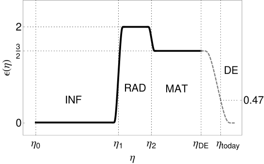
Figure 1: Schematic depiction of the expansion history in terms of $\epsilon\!=\!-\dot{H}/H^{2}$ parameter, consisting of three past cosmological eras – inflation period, radiation dominated period, and matter dominated period – and the today we are in a dark energy dominated period. Time $\eta_{0}$ corresponds to beginning of inflation, $n_{1}$ to the end of inflation, $\eta_{2}$ to the time of radiation-matter equality, and $\eta_{\text{DE}}$ to the onset of dark energy domination period. Today we are at at $\epsilon_{\text{today}}\!=\!0.47$. The first two transitions are assumed to be fast in the sense that the scale of the duration of the transition $\tau$ satisfies $\tau_{i}\!\ll\!1/\mathcal{H}_{i}$. We approximate the inflationary period by an exact de Sitter one, $\epsilon_{I}\!=\!0$.

Figure 2: Schematic depiction of the evolution of the conformal Hubble rate $\mathcal{H}$ throughout the expansion history of the universe. Hubble rates at the times of transitions satisfy the hierarchy $\mathcal{H}_{0}\!\ll\!\mathcal{H}_{\text{DE}}\!\ll\!\mathcal{H}_{2}\!\ll\!\mathcal{H}_{1}$. As in Fig. 1, time $\eta_{0}$ denotes the beginning of inflation, time $\eta_{1}$ the end of inflation, $\eta_{2}$ the end of radiation and beginning of matter dominated period (radiation-matter equality), and time $\eta_{\text{DE}}$ denotes the onset of dark energy domination.

III Scalar field model

This section introduces the model of a nonminimally coupled massive scalar field on cosmological space-time studied in this work. The quantization of the scalar on FLRW backgrounds is outlined, and the main quantities to be calculated – expectation values of the energy-momentum tensor components – are defined. The choice of initial state is discussed.

The action for the massive nonminimally coupled scalar on curved space-time is

$$S_{\phi}=\int\!d^{D}\!x\,\sqrt{-g}\,\Biggl{[}-\frac{1}{2}g^{\mu\nu}\partial_{\mu}\phi\partial_{\nu}\phi-\frac{1}{2}m^{2}\phi^{2}-\frac{1}{2}\xi R\phi^{2}\Biggr{]}\,,$$ (11)

where $m$ is the scalar field mass, and $\xi$ is the nonminimal coupling constant. Note that the sign convention we use implies $\xi_{c}=(D\!-\!2)/[4(D\!-\!1)]\xrightarrow{D\rightarrow 4}1/6$ is the conformal coupling.

III.1 Quantization on FLRW

On a FLRW background the Lagrangian density takes the form

$$\mathcal{L}_{\phi}=\frac{a^{D-2}}{2}\bigg{[}\bigl{(}\phi^{\prime}\bigr{)}^{2}-\bigl{(}\vec{\nabla}\phi\bigr{)}^{2}-(ma)^{2}\phi^{2}-\xi a^{2}R\,\phi^{2}\bigg{]}\,.$$ (12)

In order to quantize this field we need to switch to the Hamilton formalism. First we define a canonically conjugate momentum,

$$\pi(x)=\frac{\partial\mathcal{L}_{\phi}}{\partial\phi^{\prime}(x)}=a^{D-2}(\eta)\phi^{\prime}(x)\,,$$ (13)

and then the Hamiltonian via the Legendre transform,

$$H[\phi,\pi;\eta)={} \int\!d^{D-1}x\Bigl{[}\pi(x)\phi^{\prime}(x)-\mathcal{L}_{\phi}(x)\Bigr{]}$$

$$={} \frac{a^{D-2}}{2}\int\!d^{D-1}x\Bigl{[}a^{4-2D}\pi^{2}+\bigl{(}\vec{\nabla}\phi\bigr{)}^{2}+(ma)^{2}\phi^{2}+\xi a^{2}R\,\phi^{2}\Bigr{]}\,.$$ (14)

Next we promote $\phi$ and $\pi$ to operators, and their Poisson brackets to commutators,

$$\bigl{[}\hat{\phi}(\eta,\vec{x}),\hat{\pi}(\eta,\vec{x}^{\,\prime})\bigr{]}=i\delta^{D-1}(\vec{x}\!-\!\vec{x}^{\,\prime})\,,$$ (15)

$$\bigl{[}\hat{\phi}(\eta,\vec{x}),\hat{\phi}(\eta,\vec{x}^{\,\prime})\bigr{]}=0=\bigl{[}\hat{\pi}(\eta,\vec{x}),\hat{\pi}(\eta,\vec{x}^{\,\prime})\bigr{]}\,.$$ (16)

The Hamiltonian operator defined as

$$\hat{H}(\eta)=H\bigl{[}\hat{\phi},\hat{\pi};\eta\bigr{)}$$ (17)

now determines the dynamics via Heisenberg equations for the field operators,

$$\hat{\phi}^{\prime}(\eta,\vec{x})={} i\bigl{[}\hat{H}(\eta),\hat{\pi}(\eta,\vec{x})\bigr{]}=a^{2-D}(\eta)\,\hat{\pi}(\eta,\vec{x})\,,$$ (18)

$$\hat{\pi}^{\prime}(\eta,\vec{x})={} i\bigl{[}\hat{H}(\eta),\hat{\phi}(\eta,\vec{x})\bigr{]}=a^{D-2}(\eta)\Bigl{[}\vec{\nabla}^{2}-(ma)^{2}-\xi a^{2}(\eta)R(\eta)\Bigr{]}\hat{\phi}(\eta,\vec{x})\,.$$ (19)

These two combined together yield the equation of motion for the field operator

$$\Biggl{\{}\frac{\partial^{2}}{\partial\eta^{2}}+(D\!-\!2)\mathcal{H}\frac{\partial}{\partial\eta}-\vec{\nabla}^{2}+(ma)^{2}+(D\!-\!1)\xi\Bigl{[}2\mathcal{H}^{\prime}+(D\!-\!2)\mathcal{H}^{2}\Bigr{]}\Biggr{\}}\hat{\phi}(x)=0\,,$$ (20)

where $\vec{\nabla}^{2}\!=\!\sum_{i}\partial_{i}^{2}$ is the Laplace operator. This is just a Klein-Gordon equation,

$$\Bigl{[}\square-m^{2}-\xi R\Bigr{]}\hat{\phi}=0\,,$$ (21)

specialized to FLRW, where $\square\!=\!g^{\mu\nu}\nabla_{\mu}\nabla_{\nu}\!=\!(-g)^{-1/2}\partial_{\mu}[(-g)^{1/2}g^{\mu\nu}\partial_{\nu}]$ is the d’Alembert operator. This equation is standardly analyzed in Fourier (comoving momentum) space,

$$\hat{\phi}(\eta,\vec{x})=a^{\frac{2-D}{2}}\int\!\frac{d^{D-1}k}{(2\pi)^{\frac{D-1}{2}}}\Biggl{[}e^{i\vec{k}\cdot\vec{x}}U(\eta,k)\,\hat{b}(\vec{k})+e^{-i\vec{k}\cdot\vec{x}}U^{*}(\eta,k)\,\hat{b}^{{\dagger}}(\vec{k})\Biggr{]}\,,$$ (22)

where $\hat{b}(\vec{k})$ and $\hat{b}^{\dagger}(\vec{k})$ are the annihilation and creation operators, respectively, which satisfy the following commutation relations,

$$\bigl{[}\hat{b}(\vec{k}),\hat{b}^{{\dagger}}(\vec{k}^{\,\prime})\bigr{]}=\delta^{D-1}(\vec{k}\!-\!\vec{k}^{\,\prime})\,,$$ (23)

$$\bigl{[}\hat{b}(\vec{k}),\hat{b}(\vec{k}^{\,\prime})\bigr{]}=0=\bigl{[}\hat{b}^{{\dagger}}(\vec{k}),\hat{b}^{{\dagger}}(\vec{k}^{\,\prime})\bigr{]}\,,$$ (24)

and $U(k,\eta)$ is the mode function. Note the $a^{\frac{2-D}{2}}$ factor taken out in the definition of the Fourier transform (22). The commutation relations (15-16) and (23-24) require the Wronskian of the mode function to be normalized as,

$$U(k,\eta)U^{\prime*}(k,\eta)-U^{\prime}(k,\eta)U^{*}(k,\eta)=i\,.$$ (25)

The equation of motion satisfied by the mode function is the one for a harmonic oscillator with a time dependent frequency,

$$U^{\prime\prime}(k,\eta)+\Bigl{[}k^{2}+\mathcal{M}^{2}(\eta)\Bigr{]}U(k,\eta)=0\,,$$ (26)

where

$$\mathcal{M}^{2}=m^{2}a^{2}-\frac{1}{4}\Bigl{[}D\!-\!2\!-\!4\xi(D\!-\!1)\Bigr{]}\Bigl{[}2\mathcal{H}^{\prime}+(D\!-\!2)\mathcal{H}^{2}\Bigr{]}\,.$$ (27)

The state $|\Omega\rangle$ that we choose to examine we pick to be the one annihilated by the annihilation operator, $\hat{b}(\vec{k})|\Omega\rangle=0$, which implies there is no classical condensate (hence the name spectator),

$$\langle\Omega|\hat{\phi}(t,\vec{x})|\Omega\rangle=0\,.$$ (28)

This state respects the symmetries of the background space-time, namely homogeneity and isotropy, which is evident from requiring the mode function to depend only on the modulus of the comoving momentum. In order to completely specify this state one needs to specify the initial conditions for the mode function (initial state), which we comment upon in subsection III.3.

III.2 Energy-momentum tensor

The energy-momentum tensor operator is defined as

$$\hat{T}_{\mu\nu}(x)={} \left.\frac{-2}{\sqrt{-g}}\frac{\delta S_{\phi}[\phi,g^{\mu\nu}]}{\delta g^{\mu\nu}(x)}\right|_{\phi\rightarrow\hat{\phi}}$$

$$={} \partial_{\mu}\hat{\phi}(x)\,\partial_{\nu}\hat{\phi}(x)-\frac{1}{2}g_{\mu\nu}(x)\Bigl{[}g^{\alpha\beta(x)}\partial_{\alpha}\hat{\phi}(x)\,\partial_{\beta}\hat{\phi}(x)\Bigr{]}-\frac{m^{2}}{2}g_{\mu\nu}(x)\hat{\phi}^{2}(x)$$

$$+\xi\Bigl{[}G_{\mu\nu}(x)-\nabla_{\mu}\nabla_{\nu}+g_{\mu\nu}(x)\square\Bigr{]}\hat{\phi}^{2}(x)\,,$$ (29)

where $G_{\mu\nu}=R_{\mu\nu}\!-\!\frac{1}{2}g_{\mu\nu}R$ is the Einstein tensor, $\nabla$ denotes the covariant derivative, and $\square=g^{\mu\nu}\nabla_{\mu}\nabla_{\nu}$ is the covariant d’Alembertian operator. The expectation value of the energy momentum tensor operator with respect to the state defined in the previous section is diagonal, and is conveniently expressed in terms of energy density and pressure,

$$\rho_{Q}={} \frac{1}{a^{2}}\langle\Omega|\hat{T}_{00}|\Omega\rangle$$

$$={} \frac{a^{-D}}{(4\pi)^{\frac{D-1}{2}}\,\Gamma\!\left(\frac{D-1}{2}\right)}\int\limits_{0}^{\infty}\!\!dk\,k^{D-2}\Biggl{\{}2k^{2}|U|^{2}-\frac{1}{2}\bigl{[}D\!-\!2\!-\!4\xi(D\!-\!1)\bigr{]}\mathcal{H}^{\prime}|U|^{2}$$

$$+2m^{2}a^{2}|U|^{2}-\frac{1}{2}\bigl{[}D\!-\!2\!-\!4\xi(D\!-\!1)\bigr{]}\mathcal{H}\frac{\partial}{\partial\eta}|U|^{2}+\frac{1}{2}\frac{\partial^{2}}{\partial\eta^{2}}|U|^{2}\Biggr{\}}\,,$$ (30)

$$\delta_{ij}p_{Q}={} \frac{1}{a^{2}}\langle\Omega|\hat{T}_{ij}|\Omega\rangle$$

$$={} \frac{\delta_{ij}a^{-D}}{(4\pi)^{\frac{D-1}{2}}\,\Gamma\!\left(\frac{D-1}{2}\right)}\int\limits_{0}^{\infty}\!\!dk\,k^{D-2}\Biggl{\{}\frac{2k^{2}}{(D\!-\!1)}|U|^{2}-\frac{1}{2}\bigl{[}D\!-\!2\!-\!4\xi(D\!-\!1)\bigr{]}\mathcal{H}^{\prime}|U|^{2}$$

$$-\frac{1}{2}\bigl{[}D\!-\!2\!-\!4\xi(D\!-\!1)\bigr{]}\mathcal{H}\frac{\partial}{\partial\eta}|U|^{2}+\frac{(1\!-\!4\xi)}{2}\frac{\partial^{2}}{\partial\eta^{2}}|U|^{2}\Biggr{\}}\,,$$ (31)

where we have used the equation of motion (26) to write

$$|U^{\prime}|^{2}=\bigl{(}k^{2}+\mathcal{M}^{2}\bigr{)}|U|^{2}+\frac{1}{2}\frac{\partial^{2}}{\partial\eta^{2}}|U|^{2}\,,$$ (32)

and eliminate $|U^{\prime}|^{2}$ in favor of $|U|^{2}$ and its derivatives. We can take some derivatives out of the integral to write the (30) and (31) in a convenient way

$$\rho_{Q}={} \frac{a^{-D}}{(4\pi)^{\frac{D-1}{2}}\,\Gamma\!\left(\frac{D-1}{2}\right)}\Biggl{\{}2\,\mathcal{I}_{1}+\Biggl{[}2(ma)^{2}-\frac{1}{2}\bigl{[}D\!-\!2\!-\!4\xi(D\!-\!1)\bigr{]}\bigl{[}\mathcal{H}^{\prime}+\mathcal{H}\partial_{\eta}\bigr{]}+\frac{1}{2}\partial_{\eta}^{2}\Biggr{]}\mathcal{I}_{0}\Biggr{\}}\,,$$ (33)

$$p_{Q}={} \frac{a^{-D}}{(4\pi)^{\frac{D-1}{2}}\,\Gamma\!\left(\frac{D-1}{2}\right)}\Biggl{\{}\frac{2\,\mathcal{I}_{1}}{(D\!-\!1)}-\Biggl{[}\frac{1}{2}\bigl{[}D\!-\!2\!-\!4\xi(D\!-\!1)\bigr{]}\bigl{[}\mathcal{H}^{\prime}+\mathcal{H}\partial_{\eta}\bigr{]}+\frac{(1\!-\!4\xi)}{2}\partial_{\eta}^{2}\Biggr{]}\mathcal{I}_{0}\Biggr{\}}\,,$$ (34)

where we have defined the two integrals,

$$\mathcal{I}_{n}=\int\limits_{0}^{\infty}\!dk\,k^{D-2+2n}\,|U(k,\eta)|^{2}\,,\qquad n=0,1\,.$$ (35)

Finding a good approximation for these integrals is one of the two main technical tasks of this work.

III.3 Choice of state

Understanding how the choice of the initial state affects our final results is important, and this is what we discuss next at some length. We assume that the Universe starts in a natural state defined on a global equal-time hyper-surface $\Sigma_{0}$ as the Chernikov-Tagirov-Bunch-Davies (CTBD) vacuum state in the ultraviolet (UV). This means that the mode function reduces to the flat space form in the deep UV,

$$U(k,\eta)\rightarrow\frac{e^{-ik\eta}}{\sqrt{2k}}\,,$$ (36)

(a more precise statement is given in Appendix A). Furthermore, we assume the state is suitably regulated in the infrared (on super-Hubble wavelengths). That is namely necessary to regulate the infrared (IR) modes since attempting to impose the usual Bunch-Davies condition on the infrared modes would produce unphysical infrared divergences in the initial one-loop energy-momentum tensor. Infrared states can be regulated in various ways: (i) by choosing the global CTBD vacuum state associated with the epoch that precedes inflation in which the CTBD state is regular, (ii) by making the Universe’s (initial) equal-time hyper-surface compact, or (iii) by introducing a comoving IR cutoff. The first prescription can be achieved by e.g. assuming a pre-inflationary radiation epoch Janssen:2009nz ; Glavan:2014uga , while the second on by imposing a positive constant spatial curvature ($\kappa\!>\!0$) on $\Sigma_{0}$ or by making $\Sigma_{0}$ compact by imposing periodic boundary conditions (in the former case $\Sigma_{0}$ is a three-dimensional sphere $S^{3}$ while in the latter case $\Sigma_{0}$ is a 3-dimensional torus $T^{3}$). The third option is technically perhaps the simplest, and we employ it in this work. It should be stressed that the point of view on this regularization is not to throw away the deep IR modes below the cutoff on principal grounds, but rather that they are smoothly suppressed under this scale and contribute negligibly to the observables. Then the leading approximation to this case is to introduce a sharp cutoff. The deep IR suppression can be attributed to some physical process during or before inflation, or can be viewed as an approximation to the state obtained by placing the Universe in a co-moving box. One can show Tsamis:1992xa that, to leading order in powers of the IR comoving cutoff $k_{0}$, (expectation values of) physical observables are correctly reproduced by the sudden cutoff approximation.

All these methods qualitatively agree. For (i) and (ii) this was shown in Janssen:2009nz in the sense that qualitative dependence on the relevant physical scale is the same, where in the case of a pre-inflationary radiation epoch the relevant physical scale is the Hubble parameter at the radiation-inflation transition, in the case when $\Sigma_{0}\equiv S^{3}$ the relevant physical scale is $\sqrt{\kappa}$ and when $\Sigma_{0}\equiv T^{3}$ the relevant physical scale is the comoving length of the torus $L$. Note that the three aforementioned ways of regulating the infrared correspond to three (very) different physical situations.

Here we use the simple cutoff regularization – we effectively remove the modes below certain pivotal mode $k_{0}$. In practice this is implemented by cutting of the integration of $\mathcal{I}_{n}$ integrals (35) at $k_{0}$,

$$\mathcal{I}_{n}\approx\int\limits_{k_{0}}^{\infty}\!dk\,k^{D-2+2n}|U(k,\eta)|^{2}\,.$$ (37)

In the limit of very small $k_{0}$ this can be shown to be equivalent (up to corrections suppressed as $k_{0}^{2}$) to (i) mentioned above, with $k_{0}$ identified with $2\pi/L$, and is shown to be equivalent to (ii) here in Sec. VII by comparison to Janssen:2009nz ; Glavan:2014uga . The main point we are trying to make here is that, for a large class of initial states that are regular in the infrared one will get answers that qualitatively agree with the results obtained in this work, hence making the results of our analysis quite generic, i.e. to a large extent independent on the choice of the initial state.

IV Evolution of the mode function

The two main technical tasks of this work are (i) to solve for the time evolution of the mode function (26) as it evolves through cosmological eras, and (ii) to perform the integrals (30) and (31) over these mode functions to obtain the backreaction energy density and pressure. This section discusses these two issues from a more general point of view. The mode function is organized in a convenient way. Relevant integration interval is identified, and a sudden transition approximation introduced for the contributing modes. These considerations simplify following computations significantly.

IV.1 Bogolyubov coefficients

When it comes to the evolution of the mode function, unfortunately, exact results are known only for a handful of FLRW backgrounds. There is a way to write down a general solution for an arbitrary FLRW background, valid for all momentum scales Tsamis:2002qk , but it is difficult to make use of it practically. Luckily, for periods of constant $\epsilon$ (out of which most of the history of expansion consists, Fig. 1) the exact solutions are known in the massless limit, A convenient way to express them is in therms of Chernikov-Tagirov-Bunch-Davies (CTBD) mode function Chernikov:1968zm ; Bunch:1978yq ,

$$u_{\epsilon}(k,\eta)=\sqrt{\frac{\pi}{4|1\!-\!\epsilon|\mathcal{H}}}\,H_{\nu}^{(1)}\Bigl{(}\frac{k}{(1\!-\!\epsilon)\mathcal{H}}\Bigr{)}\,,$$ (38)

where the index of the Hankel function of the first kind $H_{\nu}^{(1)}$ is

$$\nu=\sqrt{\frac{1}{4}+\frac{(D\!-\!2\epsilon)}{4(1\!-\!\epsilon)^{2}}\bigl{[}D\!-\!2\!-\!4\xi(D\!-\!1)\bigr{]}}\,.$$ (39)

These functions are defined to reduce to the positive-frequency form (218) in the UV, and the IR is defined as an analytic continuation of the UV. The other linearly independent solution is a complex conjugate of (38). In the massive case, exact solutions are not known for constant $\epsilon$ periods, except in a few notable cases (de Sitter, and radiation dominated universe). Nevertheless, there is a way of making a controlled expansion of this function in the small ratio $m/H$ with which we will be concerned, which is sufficient for our purposes. This expansion is presented in Section VI.

Generally, the full mode function during a given constant $\epsilon$ period will be a linear combination of the CTBD mode functions,

$$U_{\epsilon}(k,\eta)=\alpha_{\epsilon}(k)u_{\epsilon}(k,\eta)+\beta_{\epsilon}(k)u_{\epsilon}^{*}(k,\eta)\,.$$ (40)

Coefficients $\alpha(k)$ and $\beta(k)$ are called the Bogolyubov coefficients, and they have to satisfy

$$|\alpha(k)|^{2}-|\beta(k)|^{2}=1\,,$$ (41)

as dictated by the Wronskian normalization (25). They are determined for each era by the initial conditions at the beginning of the given era, which are in turn given by the details of the transition from one era to another.

If $\tau$ is a small time scale of the transition between periods, then for momenta above this scale the Bogolyubov coefficients must reduce to

$$\alpha(k)\xrightarrow{k\rightarrow\infty}1\,,\qquad\beta(k)\xrightarrow{k\rightarrow\infty}0\,,$$ (42)

nonadiabatically, meaning faster than any power of $1/k$. This is provided that the initial condition is of adiabatic order $\infty$. Otherwise, if the initial state is of adiabatic order $n$, it retains that property during the evolution Kulsrud:1957zz . This we can also infer from considerations of Appendix A. The physical reason behind this conclusion is that the deep UV modes oscillate so fast so that their evolution is adiabatic.

In the IR, Bogolyubov coefficients are not universal as the deep UV are. On the contrary, they do depend on the details of the transition between the two periods of constant $\epsilon$. In case of a fast transition they are not so sensitive (to leading order) to the details of the transition, but rather depend just on the two periods connected by the transition. This we show in the next subsection.

IV.2 Sudden transition approximation

In case of fast transitions between constant $\epsilon$ periods, $\tau\!\ll\!1/\mathcal{H}$, the evolution of the IR modes, $k\!\ll\!1/\tau$, through the transition is well described by the so-called sudden transition approximation, where the $\epsilon$ parameter jumps discontinuously from one constant value to another. Physically, these modes are very slow compared to the transition scale, and the transition is effectively instantaneous for them. More precisely, the transition is instantaneous for the IR modes to leading order in the expansion in the transition scale $\tau$. We stress that this is an approximation for the evolution of the IR modes, not a model for the background evolution, and should not be extrapolated to UV modes.

Here we illustrate the sudden transition approximation on a specific example of transition between two periods $\epsilon_{0}$ and $\epsilon_{1}$. Let the evolution of $\epsilon$ between two periods be given by

$$\epsilon(\eta)=\left\{\begin{matrix}\epsilon_{0}&,&\eta<\eta_{0}-\frac{\tau}{2}\\ \epsilon_{\text{tr}}(\eta)&,&\eta_{0}-\frac{\tau}{2}<\eta<\eta_{0}+\frac{\tau}{2}\\ \epsilon_{1}&,&\eta>\eta_{0}+\frac{\tau}{2}\end{matrix}\right.$$ (43)

where

$$\epsilon_{\text{tr}}(\eta)=\frac{\epsilon_{0}}{2}\Biggl{[}1+\tanh\Biggl{(}\frac{1}{1+\frac{\eta-\eta_{0}}{\tau/2}}-\frac{1}{1-\frac{\eta-\eta_{0}}{\tau/2}}\Biggr{)}\Biggr{]}+\frac{\epsilon_{1}}{2}\Biggl{[}1+\tanh\Biggl{(}-\frac{1}{1+\frac{\eta-\eta_{0}}{\tau/2}}+\frac{1}{1-\frac{\eta-\eta_{0}}{\tau/2}}\Biggr{)}\Biggr{]}\,.$$ (44)

Before the transition let the full mode function be

$$U(k,\eta<\eta_{0}-\tfrac{\tau}{2})=\alpha_{0}(k)u_{0}(k,\eta)+\beta_{0}u_{0}^{*}(k,\eta)\equiv U_{0}(k,\eta)\,,$$ (45)

with some known Bogolyubov coefficients $\alpha_{0}$ and $\beta_{0}$. After the transition the mode function is

$$U(k,\eta>\eta_{0}+\tfrac{\tau}{2})=\alpha_{1}(k)u_{1}(k,\eta)+\beta_{1}u_{1}^{*}(k,\eta)\equiv U_{1}(k,\eta)\,.$$ (46)

The equation (26) we are trying to solve is the harmonic oscillator one with a time dependent frequency,

$$U^{\prime\prime}+\omega^{2}(\eta)U=0\,,$$ (47)

where

$$\omega^{2}(\eta)=k^{2}+\mathcal{M}^{2}(\eta)\,,$$ (48)

and $\mathcal{M}^{2}$ is defined in (27). One can check the WKB applicability condition $\omega^{\prime}/\omega^{2}\!\ll\!1$, and for which ranges of momenta is it satisfied,

$$\frac{\omega^{\prime}}{\omega^{2}}\sim\left\{\begin{matrix}\displaystyle\frac{\mathcal{H}^{2}}{k^{2}}\frac{1}{(k\tau)^{2}}&,&k\gg\mathcal{H}\\ \displaystyle 1/(\mathcal{H}\tau)&,&k\lesssim\mathcal{H}\end{matrix}\right.\ .$$ (49)

Since $\tau\!\ll\!1/\mathcal{H}$ by assumption, the only modes that evolve adiabatically are the ones for which at least $k>\mu\gg\mathcal{H}$.

For the modes $k\!<\!\mu$ another approximation applies. There $1/\tau$ is the largest scale in the hierarchy, and we can expand the evolution in powers of $\tau$. We do this by expanding $\epsilon(\eta)$ function (44),

$$\epsilon(\eta)\approx\epsilon_{0}\,\theta(\eta_{0}\!-\!\eta)+\epsilon_{1}\,\theta(\eta\!-\!\eta_{0})+\mathcal{O}(\tau)\,.$$ (50)

Now it is straightforward to match the two solutions (45) and (46), which are just the continuity conditions for the mode function and its derivative,

$$U_{0}(k,\eta_{0})=U_{1}(k,\eta_{0})\,,\qquad U_{0}^{\prime}(k,\eta_{0})=U_{1}^{\prime}(k,\eta_{0})\,.$$ (51)

Solving these conditions for Bogolyubov coefficients yields

$$\alpha_{1}(k)={} -i\Bigl{[}U_{0}(k,\eta_{0})u_{1}^{\prime*}(k,\eta_{0})-U_{0}^{\prime}(k,\eta_{0})u_{1}^{*}(k,\eta_{0})\Bigr{]}+\mathcal{O}(\tau)\,,$$ (52)

$$\beta_{1}(k)={} i\Bigl{[}U_{0}(k,\eta_{0})u_{1}^{\prime}(k,\eta_{0})-U_{0}^{\prime}(k,\eta_{0})u_{1}(k,\eta_{0})\Bigr{]}+\mathcal{O}(\tau)\,.$$ (53)

These two formulas comprise the sudden transition approximation for the Bogolyubov coefficients and the evolution of the mode function.

V Energy density and pressure integrals

In this section we analyze the integrals (35) on general grounds. They cannot be evaluated exactly (except for very simple mode functions Glavan:2013mra ), and we have to resort to approximation schemes. We first organize the integrand in a way which separates the part containing all the UV divergences (among other contributions), and the UV finite part containing possibly relevant IR contributions. The contributions from different scales, i.e. different integration intervals are examined, and the relevant interval where the dominant contribution comes from is identified. The analysis presented here greatly facilitates the evaluation of integrals (35), especially since we get away with not evaluating certain parts of integrals explicitly (as was done in Glavan:2014uga ).

V.1 Organizing the integrand

The integrands of integrals (35) contain the mode function only as a modulus $|U(k,\eta)|^{2}$, which can be written out in terms of the CTBD mode functions of a given constant $\epsilon$ period,

$$|U(k,\eta)|^{2}=|u(k,\eta)|^{2}+2|\beta(k)|^{2}|u(k,\eta)|^{2}+\alpha(k)\beta^{*}(k)u^{2}(k,\eta)+\alpha^{*}(k)\beta(k)[u^{*}(k,\eta)]^{2}\,,$$ (54)

where (41) was used. In the deep UV Bogolyubov coefficients reduce to (42) faster than power law (at least exponentially). Therefore, the UV divergent structure of integrals (35) is completely captured by the $|u(k,\eta)|^{2}$ on the right in (54). We split the integrals into two parts,

$$\mathcal{I}_{n}=\mathcal{I}^{\text{CTBD}}_{n}+\mathcal{I}^{\text{Bog.}}_{n}\,,$$ (55)

where the CTBD part is

$$\mathcal{I}^{\text{CTBD}}_{n}=\int\limits_{k_{0}}^{\infty}\!dkk^{D-2+2n}|u(k,\eta)|^{2}\,,$$ (56)

which contains all the UV divergences, and the Bogolyubov part,

$$\mathcal{I}_{n}^{\text{Bog.}}=\int\limits_{k_{0}}^{\infty}\!dk\,k^{2+2n}\,Z_{\text{Bog.}}(k,\eta)\,,$$ (57)

where the integrand is

$$Z_{\text{Bog.}}(k,\eta)=2|\beta(k)|^{2}|u(k,\eta)|^{2}+\alpha(k)\beta^{*}(k)u^{2}(k,\eta)+\alpha^{*}(k)\beta(k)[u^{2}(k,\eta)]^{*}\,.$$ (58)

Note that we take $D\!=\!4$ limit in the Bogolyubov part, since it is manifestly UV finite because of the properties of the Bogolyubov coefficients (42), which simplifies its evaluation.

We can immediately say a lot about the CTBD contribution (56). The way to compute it is to first split it in the UV and IR parts by introducing a UV cutoff $\mu\!\gg\!\mathcal{H}$,

$$\mathcal{I}_{n}^{\text{CTBD}}=\mathcal{I}_{n}^{\text{CTBD,UV}}+\mathcal{I}_{n}^{\text{CTBD,IR}}=\int\limits_{\mu}^{\infty}\!dkk^{D-2+2n}|u(k,\eta)|^{2}+\int\limits_{k_{0}}^{\mu}\!dkk^{2+2n}|u(k,\eta)|^{2}\,.$$ (59)

Its UV part needs to be regularized and then renormalized as is outlined in Appendix A, and its contribution is given in (241-242) and (246). Note that this UV contribution is dependent on the fiducial cutoff $\mu$ introduced by hand. That dependence cancels exactly with the opposite one coming from the IR contribution (which can be evaluated in $D\!=\!4$ from the start). This computation is performed explicitly in subsection VII.1 for inflationary era.

The only dimensionful quantities the CTBD part can depend on are the evolving Hubble rate and mass, and possibly on the IR regulator. The dependence on the regulator actually must cancel out with same contribution from the Bogolyubov part. The total dependence on the regulator in the final answer can only come from the CTBD part and it must have the same structure as the initial state Ford:1977in . Therefore, in the small mass limit we can represent possible contributions to energy density and pressure as

$$\frac{\mathcal{H}^{4}}{a^{4}}\biggl{\{}\ln(a)\Bigl{[}\#_{1}+\#_{2}\Bigl{(}\frac{ma}{\mathcal{H}}\Bigr{)}^{\!2}+\#_{3}\Bigl{(}\frac{ma}{\mathcal{H}}\Bigr{)}^{\!4}+\dots\Bigr{]}+\Bigl{[}\#_{4}+\#_{5}\Bigl{(}\frac{ma}{\mathcal{H}}\Bigr{)}^{\!2}+\#_{6}\Bigl{(}\frac{ma}{\mathcal{H}}\Bigr{)}^{\!4}+\dots\Bigr{]}\biggr{\}}\,,$$ (60)

where $\#_{i}$’s stand for some numerical coefficients of order one. This contribution is not relevant during the radiation or matter period. Its magnitude is tiny compared to the background. In matter period it also redshifts faster than the background. In radiation period it does not, rather it redshifts at the same rate as the background fluid ($\mathcal{H}^{4}a^{-4}\ln(a)$ term is absent in this case), but its magnitude is tiny. The contribution from this CTBD part is always negligible compared to the background, and therefore we can neglect it. If there is a large effect, it must lie in the Bogolyubov part. That contribution we analyze generally in the next subsection.

V.2 Bogolyubov part

We would like to argue on general grounds about the contributions from different momentum scales to this integral. For the sake of simplicity, consider the transition between two periods of constant $\epsilon$. Before the transition, during period $\epsilon_{0}$, the state was the CTBD one ($\alpha_{0}\!=\!1$, $\beta_{0}\!=\!0$). The state after the transition, during period $\epsilon_{1}$ is dictated by the transition between periods, which is assumed to be fast ($\tau_{0}\!\ll\!1/\mathcal{H}_{0}$). We examine the two cases for the second period separately – the decelerated case ($\epsilon_{1}\!>\!1$), and the accelerated case ($\epsilon_{1}\!<\!1$).

V.2.1 Decelerating period

After the transition to the decelerating period the time evolving Hubble rate $\mathcal{H}$ drops below the one at the transition point $\mathcal{H}_{0}$ (see Fig. 2) and eventually the hierarchy of scales depicted in Figure 3 is reached. This happens some time after the transition, which is the regime we are interested in. We split the integration into three intervals, separated by $\mu_{0}$ and $\mu$, according to this hierarchy. The modes in the highest interval $k>\mu_{0}$ contribute negligibly since the Bogolyubov coefficients are nonadiabatically suppressed there ($\beta\sim e^{-\tau k}$).

Figure 3: Hierarchy of scales after the transition to a decelerating period

The contribution of the middle interval can be estimated rather generally. We start by noting that

$$\bigl{|}\mathcal{I}_{n}^{\text{Bog.,mid.}}\bigr{|}=\left|\int\limits_{\mu}^{\mu_{0}}\!dk\,k^{2+2n}\,Z_{\text{Bog.}}(k,\eta)\right|$$

$$\hskip 14.22636pt\leq 2\int\limits_{\mu}^{\mu_{0}}\!dk\,k^{2+2n}\Bigl{[}\bigl{|}\beta_{1}(k)\bigr{|}^{2}+\bigl{|}\alpha_{1}(k)\bigr{|}\bigl{|}\beta_{1}(k)\bigr{|}\Bigr{]}\bigl{|}u_{1}(k,\eta)\bigr{|}^{2}\,.$$ (61)

The time dependent BD mode function may be expanded asymptotically as in (230) since $k\gg\mathcal{H}\gg ma$ on this interval,

$$|u_{1}(k,\eta)|^{2}\approx\frac{1}{2k}\Biggl{\{}1+\frac{\mathcal{H}^{2}}{4k^{2}}\Bigl{[}1+\mathcal{O}\Bigl{(}\frac{ma}{\mathcal{H}}\Bigr{)}^{\!2}\Bigr{]}+\mathcal{O}\Bigl{(}\frac{\mathcal{H}}{k}\Bigr{)}^{\!4}\Biggr{\}}$$ (62)

The momentum scales in question are much smaller than the scale of the transition $1/\tau$, so the Bogolyubov coefficients are well approximated by the sudden transition ones, and depend on three quantities: $k$, $\mathcal{H}_{0}$, $ma_{0}$. Since we are interested in the small mass limit we may expand the Bogolyubov coefficients in powers of $ma_{0}/\mathcal{H}_{0}$,

$$\beta_{1}(k,\mathcal{H}_{0},ma_{0})\approx\beta_{1}\Bigl{(}\frac{k}{\mathcal{H}_{0}}\Bigr{)}\Bigl{[}1+\mathcal{O}\Bigl{(}\frac{ma_{0}}{\mathcal{H}_{0}}\Bigr{)}\Bigr{]}\,,$$ (63)

and analogously for $\alpha_{1}$, so to leading order they depend only on the ratio $k/\mathcal{H}_{0}$. Therefore, we can approximate (61) with

$$\bigl{|}\mathcal{I}^{\text{Bog.,mid.}}_{n}\bigr{|}\lesssim\int\limits_{\mu}^{\mu_{0}}\!dk\,k^{1+2n}\Biggl{[}\Bigl{|}\beta_{1}\Bigl{(}\frac{k}{\mathcal{H}_{0}}\Bigr{)}\Bigr{|}^{2}+\Bigl{|}\alpha_{1}\Bigl{(}\frac{k}{\mathcal{H}_{0}}\Bigr{)}\Bigr{|}\Bigl{|}\beta_{1}\Bigl{(}\frac{k}{\mathcal{H}_{0}}\Bigr{)}\Bigr{|}\Biggr{]}\,.$$ (64)

Making a variable substitution $K=k/\mathcal{H}_{0}$ puts this integral into a form which is suitable for further approximation,

$$\bigl{|}\mathcal{I}^{\text{Bog.,mid.}}_{n}\bigr{|}\lesssim\mathcal{H}_{0}^{2+2n}\int\limits_{\mu/\mathcal{H}_{0}}^{\mu_{0}/\mathcal{H}_{0}}\!\!dK\,K^{1+2n}\Bigl{[}\bigl{|}\beta_{1}(K)\bigr{|}^{2}+\bigl{|}\alpha_{1}(K)\bigr{|}\bigl{|}\beta_{1}(K)\bigr{|}\Bigr{]}\,.$$ (65)

The integrand is now dimensionless, and the limits of integration are $\mu/\mathcal{H}_{0}\!\ll\!1$, and $\mu_{0}/\mathcal{H}_{0}\!\gg\!1$, so we may perform (asymptotic) expansions in these limits. It might happen so that the leading order contribution is dominated by one of the cutoffs, but this contribution (and in fact any other cutoff dependent one) must cancel with the opposite contribution from another part of the full integral. Although tedious, this can be checked explicitly as was done in Glavan:2014uga . Therefore, what we are interested in is the contribution independent off $\mu_{0}$ and $\mu$, since that is the only one that remains after all the parts are added up. That contribution has the following form,

$$\bigl{|}\mathcal{I}_{n}^{\text{Bog.,mid.}}\bigr{|}\sim\#\mathcal{H}_{0}^{2+2n}\,.$$ (66)

This gives the contribution to the energy density (and momentum) of the form

$$\rho\sim\#\frac{\mathcal{H}_{0}^{4}}{a^{4}}\,.$$ (67)

It is just a radiation-like contribution, and redshifts away faster than the background (or at the same rate in the case of radiation era). Therefore we may safely neglect it as long as it is not too big before the start of radiation period.

The lower part of the integral has a chance to contribute something that does not redshift away faster than the background. Its exact contribution is not so straightforward to estimate, but if there is an interesting effect to be found it derives from this contribution. Therefore, it is the only one we need to examine, which we do in Sec. VII. For completeness, next we examine the accelerated case, $\epsilon_{1}\!<\!1$.

V.2.2 Accelerating period

In the case of universe transitioning from one period of constant $\epsilon_{0}$ where the scalar was in a CTBD state, to an accelerating period of constant $\epsilon_{1}\!<\!1$, where the transition was fast, we soon reach a hierarchy of scales shown in Case A of Fig. 4, and afterwards the one in Case B, as the conformal Hubble rate continues to grow. We treat these two cases separately.

(a) Case A

(b) Case B

Figure 4: Hierarchy of scales after the transition to accelerating period; Case A: some time after the transition, Case B: very long after the transition.

Case A

The hierarchy of scales in this case is depicted on the left of Fig. 4. The contribution from the modes $k\!>\!\mu_{0}$ is negligible because of the nonadiabatic suppression of Bogolyubov coefficients, just as in the decelerating case.

The contribution from the middle interval can be estimated as

$$\bigl{|}\mathcal{I}_{n}^{\text{Bog.,mid.}}\bigr{|}\leq 2\int\limits_{\mu_{0}}^{\mu}\!dk\,k^{2+2n}\Bigl{[}\bigl{|}\beta_{1}(k)\bigr{|}^{2}+\bigl{|}\alpha_{1}(k)\bigr{|}\bigl{|}\beta_{1}(k)\bigr{|}\Bigr{]}\bigl{|}u_{1}(k,\eta)\bigr{|}^{2}$$ (68)

in a similar way as in the decelerating case. Here, because of the hierarchy of scales, we may expand the sudden transition Bogolyubov coefficients for large momenta (see Glavan:2013mra for the expansion),

$$\alpha(k)\approx{} 1+\mathcal{O}\Bigl{(}\frac{\mathcal{H}_{0}}{k}\Bigr{)}$$ (69)

$$\beta(k)\approx{} \frac{\mathcal{H}_{0}^{2}}{k^{2}}+\mathcal{O}\Bigl{(}\frac{\mathcal{H}_{0}}{k}\Bigr{)}\,.$$ (70)

The time dependent mode function depends on $k$, $\mathcal{H}$ and $ma$. Since $ma\ll k,\mathcal{H}$ we can expand away its $m$-dependence so that the leading order term depends only on $k/\mathcal{H}$ and $\mathcal{H}$. Then, using the variable substitution $K=k/\mathcal{H}$ in the middle integral we can estimate it as

$$|\mathcal{I}_{n}^{\text{Bog.,mid.}}|\leq\#\mathcal{H}_{0}^{2}\mathcal{H}^{2n+1}\int\limits_{\mu_{0}/\mathcal{H}}^{\mu/\mathcal{H}}\!dK\,K^{2n}|u_{1}(k,\mathcal{H})|^{2}\Bigl{[}1+\mathcal{O}\Bigl{(}\frac{\mathcal{H}}{\mathcal{H}_{0}}\Bigr{)}\Bigr{]}\,.$$ (71)

As in the decelerating case, this integral can be expanded for small lower and large upper limit. Neglecting as before terms dependent on the artificially introduced cutoffs, what can remain is a contribution $\#\mathcal{H}_{0}^{2}\mathcal{H}^{2n}$. Now, these contribute to energy density and pressure as $\#\mathcal{H}_{0}^{2}\mathcal{H}^{2}/a^{4}$. If the numerical coefficient is not exponentially large, this contribution is negligible compared to the background fluid energy density, and it only redshifts away faster than the background. Only the lower integrals remains to be evaluated.

Case B

In this case the reasoning of Case A applies, we just need not examine the middle integral, since here it is shifted into the region where Bogolyubov coefficients are nonadiabatically suppressed (as depicted on the right of Fig. 4), and hence contributes negligibly. One needs to examine the same (lower) interval to look for the dominant contribution.

VI Mode functions

In this section we derive the CTBD mode functions for each of the cosmological periods. Exact solutions are known for the inflationary and radiation periods. While we can perform integrals (35) over the exact inflationary mode functions, the radiation ones are too complicated, and need to be approximated. An expansion in small $m/H\!=\!ma/\mathcal{H}$ to first subleading order suffices for our goals. This expansion is performed in two ways. Firstly, the exact radiation period mode function is expanded, and the approximation valid for all momenta obtained. Secondly, the method for obtaining the approximation directly from the equation of motion (26) (without referring to the exact solution) is introduced, and the approximation for the radiation period mode function derived. This method is shown to reproduce the expansion of the exact result, which lends support for applying it in cases where the exact mode functions are not known. The matter period mode functions are not known exactly, and we apply this method in order to find its expansion to first subleading order in small mass, valid for all momenta. All the approximated mode functions derived in this section are simple enough so that integrals (35) can be performed, and the energy density and pressure of quantum backreaction computed.

VI.1 Inflationary era

Fortunately, the de Sitter inflationary period ($\epsilon_{I}\!=\!0$) CTBD mode functions are known exactly even in the massive case. The equation of motion for the mode function is

$$u^{\prime\prime}+\Bigl{[}k^{2}+(ma)^{2}-2(1\!-\!6\xi)\mathcal{H}^{2}\Bigr{]}u=0\,.$$ (72)

The positive frequency solution to this equation is

$$u_{I}(k,\eta)=\sqrt{\frac{\pi}{4\mathcal{H}}}\,H_{\nu_{I}}^{(1)}\Bigl{(}\frac{k}{\mathcal{H}}\Bigr{)}\,,$$ (73)

where

$$\nu_{I}=\sqrt{\frac{1}{4}+2(1\!-\!6\xi)-\Bigl{(}\frac{m}{H}\Bigr{)}^{2}}\,.$$ (74)

In this work we will be considering mass of the order of Hubble rate today (meaning that the ratio $m/H_{I}$ in inflation is extremely small), and nonminimal couplings $0\!>\!\xi\!\gtrsim\!-0.05$. More negative nonminimal couplings would lead to a too rapid growth of quantum fluctuations during inflation (as will be shown by the end of this subsection), and a larger mass would mean that the field becomes very massive at some point during the cosmological evolution and starts contributing like dust to the expansion (precluding it from having anything to do with DE). For most of the range of these two parameters $\nu_{I}\!>\!3/2$, which leads to an IR divergence. This divergence has to be regulated somehow, since it signals that the state chosen is unphysical. The practical method of regularization we choose is introducing a comoving IR cutoff $k_{0}$. The point of view we take on it is that it is a shortcut way of choosing a physical mode function, since the contribution of the modes below $k_{0}$ will be suppressed, and we neglect it from the start.

We will also need the small momentum ($k\!\ll\!\mathcal{H}$) expansion of the mode function in (73),

$$u_{I}(k,\eta)\approx-\frac{i}{\sqrt{\pi}}2^{\nu_{I}-1}\Gamma(\nu_{I})\mathcal{H}_{1}^{\nu_{I}-1/2}k^{-\nu_{I}}\Bigl{[}1+\mathcal{O}\Bigl{(}\frac{k}{\mathcal{H}}\Bigr{)}^{2}\Bigr{]}\,.$$ (75)

VI.2 Radiation era

In this subsection first the exact the radiation period CTBD mode function is derived, and then an expansion for $m/H\!\ll\!1$ performed (valid for all momenta). Secondly, this small mass expansion is derived directly from the equation of motion without referring to the exact solution with the help of Frobenius method. This serves to introduce the method which can be applied to cases where an exact solution is not known.

VI.2.1 Exact CTBD mode function

The CTBD mode functions for radiation period are also known in the massive case, but are unfortunately too complicated for practical analytical computations. The equation of motion for the modes is

$$u^{\prime\prime}+\Bigl{[}k^{2}+(ma)^{2}\Bigr{]}u=0\,.$$ (76)

In radiation period the scale factor and the conformal Hubble rate are related as

$$a\mathcal{H}=a_{1}\mathcal{H}_{1}\,,$$ (77)

where the quantities with index 1 refer to the values at the beginning of radiation period, so the equation (76) can be written as

$$u^{\prime\prime}+\Bigl{[}k^{2}+\frac{\overline{m}^{4}}{\mathcal{H}^{2}}\Bigr{]}u=0\,,$$ (78)

where we have defined

$$\overline{m}=\sqrt{ma_{1}\mathcal{H}_{1}}\,.$$ (79)

By making a variable substitution

$$s=\frac{i\,\overline{m}^{2}}{\mathcal{H}^{2}}\,,$$ (80)

the equation can be put in the form

$$\Biggl{\{}\frac{\partial^{2}}{\partial s^{2}}+\biggl{[}-\frac{1}{4}-\frac{i}{4s}\Bigl{(}\frac{k}{\overline{m}}\Bigr{)}^{2}+\frac{3}{16s^{2}}\biggr{]}\Biggr{\}}\bigl{(}s^{1/4}u\bigr{)}=0\,,$$ (81)

which is a Whittaker equation gradshteyn2007 ,

$$\Biggl{\{}\frac{\partial^{2}}{\partial s^{2}}+\biggl{[}-\frac{1}{4}+\frac{\lambda}{s}+\frac{\frac{1}{4}-\mu^{2}}{s^{2}}\biggr{]}\Biggr{\}}\bigl{(}s^{-1/4}u\bigr{)}=0\,,$$ (82)

with coefficients

$$\lambda=-\frac{i}{4}\Bigl{(}\frac{k}{\overline{m}}\Bigr{)}^{2}\ ,\qquad\mu=\frac{1}{4}\,.$$ (83)

The properly normalized (using the Wronskian 13.14.30 from NIST:DLMF ) CTBD mode function is

$$u_{R}(k,\eta)=\sqrt{\frac{\mathcal{H}}{2\overline{m}^{2}}}\ e^{-\frac{\pi k^{2}}{8\overline{m}^{2}}}\times W_{\!-\frac{ik^{2}}{4\overline{m}^{2}},\frac{1}{4}}\Bigl{(}\frac{i\,\overline{m}^{2}}{\mathcal{H}^{2}}\Bigr{)}\,,$$ (84)

where $W$ is the Whittaker function. By examining the UV expansion $k\!\rightarrow\!\infty$ of (84) (corresponding to the large parameter expansion 9.229 from gradshteyn2007 ),

$$u_{R}(k,\eta)\xrightarrow{k\rightarrow\infty}\frac{e^{-\frac{ik}{\mathcal{H}}}}{\sqrt{2k}}\times\exp\Bigl{[}\frac{i\pi}{2}+\frac{ik^{2}}{4\overline{m}^{2}}-\frac{ik^{2}}{4\overline{m}^{2}}\ln\Bigl{(}\frac{ik^{2}}{4\overline{m}^{2}}\Bigr{)}\Bigr{]}\,,$$ (85)

we see that it indeed is the positive-frequency mode function (the time-independent phase is irrelevant since it cancels out in all the physical quantities, the mode function is defined up to such a phase).

Next we want to find the expansion of this function in small parameter $ma/\mathcal{H}=\overline{m}^{2}/\mathcal{H}^{2}$, but valid for all momenta. In order to accomplish this we view the function as a function of momenta. In particular we represent it as a uniformly convergent power series in momenta. The coefficients in this expansion are functions of $m$ and $\mathcal{H}$, and them we expand in this small ratio.

It is more convenient to express the Whittaker function in terms of confluent hypergeometric functions,

$$W_{\!-\frac{ik^{2}}{4\overline{m}^{2}},\frac{1}{4}}\Bigl{(}\frac{i\overline{m}^{2}}{\mathcal{H}^{2}}\Bigr{)}={} \frac{-2\sqrt{\pi}\,e^{-\frac{i\overline{m}^{2}}{2\mathcal{H}^{2}}}}{\Gamma\left(\frac{1}{4}\!+\!\frac{ik^{2}}{4\overline{m}^{2}}\right)}\Bigl{(}\frac{i\overline{m}^{2}}{\mathcal{H}^{2}}\Bigr{)}^{\!\frac{3}{4}}{}_{1}F_{1}\Bigl{(}\frac{3}{4}\!+\!\frac{ik^{2}}{4\overline{m}^{2}};\frac{3}{2};\frac{i\overline{m}^{2}}{\mathcal{H}^{2}}\Bigr{)}$$

$$+\frac{\sqrt{\pi}\,e^{-\frac{i\overline{m}^{2}}{2\mathcal{H}^{2}}}}{\Gamma\!\left(\frac{3}{4}\!+\!\frac{ik^{2}}{4\overline{m}^{2}}\right)}\Bigl{(}\frac{i\overline{m}^{2}}{\mathcal{H}^{2}}\Bigr{)}^{\!\frac{1}{4}}{}_{1}F_{1}\Bigl{(}\frac{1}{4}\!+\!\frac{ik^{2}}{4\overline{m}^{2}};\frac{1}{2};\frac{i\overline{m}^{2}}{\mathcal{H}^{2}}\Bigr{)}\,.$$ (86)

The radius of convergence of the power series representation of the confluent hypergeometric function is infinite so we may safely examine it, and do manipulations of it,

$${}_{1}F_{1}\Bigl{(}\frac{1\!+\!\sigma}{2}\!+\!\frac{ik^{2}}{4\overline{m}^{2}};1\!+\!\sigma;\frac{i\overline{m}^{2}}{\mathcal{H}^{2}}\Bigr{)}=\sum_{n=0}^{\infty}\frac{\left(\frac{1\!+\!\sigma}{2}\!+\!\frac{ik^{2}}{4\overline{m}^{2}}\right)^{\!(n)}}{(1\!+\!\sigma)^{(n)}}\frac{1}{n!}\Bigl{(}\frac{i\overline{m}^{2}}{\mathcal{H}^{2}}\Bigr{)}^{n}\,,\qquad\Bigl{(}\sigma\!=\!\pm\frac{1}{2}\Bigr{)}\,,$$ (87)

where $(x)^{(n)}\!=\!x(x\!+\!1)(x\!+\!2)\dots(x\!+\!n\!-\!1)$ is the Pochhammer symbol. What we aim to do is to rewrite it as the power series in $k/\mathcal{H}$. In order to do this we write out the Pochhammer symbol,

$$\Bigl{(}\frac{1\!+\!\sigma}{2}+\frac{ik^{2}}{4\overline{m}^{2}}\Bigr{)}^{\!(n)}=\sum_{s=0}^{n}d_{n,s}^{(\sigma)}\Bigl{(}\frac{ik^{2}}{4\overline{m}^{2}}\Bigr{)}^{\!n-s}\,,$$ (88)

where $d$-coefficients can be determined by writing out the Pochhammer symbol. Using this the power series representation (87) of the confluent hypergeometric function can be rewritten as

$${}_{1}F_{1}\Bigl{(}\frac{1\!+\!\sigma}{2}\!+\!\frac{ik^{2}}{4\overline{m}^{2}};1\!+\!\sigma;\frac{i\overline{m}^{2}}{\mathcal{H}^{2}}\Bigr{)}=\sum_{s=0}^{\infty}\Bigl{(}\frac{ima}{\mathcal{H}}\Bigr{)}^{s}\times\sum_{n=0}^{\infty}\frac{d^{(\sigma)}_{n+s,s}}{(n\!+\!s)!\,(1\!+\!\sigma)^{(n+s)}}\Bigl{(}\frac{-k^{2}}{4\mathcal{H}^{2}}\Bigr{)}^{n}\,.$$ (89)

This power series is now straightforward to approximate this power series for small $ma/\mathcal{H}$ – we simply throw away all the terms except the first three ones,

$${}_{1}F_{1}\Bigl{(}\frac{1\!+\!\sigma}{2}\!+\!\frac{ik^{2}}{4\overline{m}^{2}};1\!+\!\sigma;\frac{i\overline{m}^{2}}{\mathcal{H}^{2}}\Bigr{)}\approx\sum_{s=0}^{3}\Bigl{(}\frac{ima}{\mathcal{H}}\Bigr{)}^{s}\times\sum_{n=0}^{\infty}\frac{d^{(\sigma)}_{n+s,s}}{(n\!+\!s)!\,(1\!+\!\sigma)^{(n+s)}}\Bigl{(}\frac{-k^{2}}{4\mathcal{H}^{2}}\Bigr{)}^{n}\,.$$ (90)

This approximation can be seen to be valid for all the ranges of momenta. For $k\gg ma$ this is just an expansion in $ma$ which is the smallest scale in the hierarchy. For $k\lesssim ma$ the function is well described by a double expansion, in $ma/\mathcal{H}$, and $k/\mathcal{H}$, so is good, it just retains more terms than necessary in this limit, which we neglect anyway. Now, we need only the first three $d$-coefficients introduced in (88),

$$d_{n,0}^{(\sigma)}=1\,,\qquad d_{n,1}^{(\sigma)}=\sum_{l=0}^{n-1}\Bigl{(}\frac{1}{2}\!+\!\sigma\!+\!l\Bigr{)}=\frac{n(n\!+\!\sigma)}{2}\,,$$ (91)

$$d_{n,2}^{(\sigma)}=\sum_{l=0}^{n-2}\sum_{j=l+1}^{n-1}\Bigl{(}\frac{1}{2}\!+\!\sigma\!+\!l\Bigr{)}\Bigl{(}\frac{1}{2}\!+\!\sigma\!+\!j\Bigr{)}=\frac{n(n\!-\!1)}{24}\Bigl{[}3n^{2}\!+\!(6\sigma\!-\!1)n\!-\!\frac{1}{4}\,\Bigr{]}\,.$$ (92)

The approximations for the confluent hypergeometric functions are then

$${}_{1}F_{1}\Bigl{(}\frac{3}{4}\!+\!\frac{ik^{2}}{4\overline{m}^{2}};\frac{3}{2};\frac{i\overline{m}^{2}}{\mathcal{H}^{2}}\Bigr{)}\approx\frac{\mathcal{H}}{k}\sin\Bigl{(}\frac{k}{\mathcal{H}}\Bigr{)}+\Bigl{(}\frac{ma}{\mathcal{H}}\Bigr{)}\times\frac{i\mathcal{H}}{2k}\sin\Bigl{(}\frac{k}{\mathcal{H}}\Bigr{)}$$

$$\hskip 56.9055pt+\Bigl{(}\frac{ma}{\mathcal{H}}\Bigr{)}^{2}\times\Biggl{\{}\Bigl{[}-\frac{1}{8}\!-\!\frac{\mathcal{H}^{2}}{4k^{2}}\!+\!\frac{\mathcal{H}^{4}}{4k^{4}}\Bigr{]}\frac{\mathcal{H}}{k}\sin\Bigl{(}\frac{k}{H}\Bigr{)}+\Bigl{[}\frac{\mathcal{H}^{2}}{6k^{2}}-\frac{\mathcal{H}^{4}}{4k^{4}}\Bigr{]}\cos\Bigl{(}\frac{k}{\mathcal{H}}\Bigr{)}\Biggr{\}}\,,$$ (93)

$${}_{1}F_{1}\Bigl{(}\frac{1}{4}\!+\!\frac{ik^{2}}{4\overline{m}^{2}};\frac{1}{2};\frac{i\overline{m}^{2}}{\mathcal{H}^{2}}\Bigr{)}\approx\cos\Bigl{(}\frac{k}{\mathcal{H}}\Bigr{)}+\Bigl{(}\frac{ma}{\mathcal{H}}\Bigr{)}\times\frac{i}{2}\cos\Bigl{(}\frac{k}{\mathcal{H}}\Bigr{)}$$

$$\hskip 56.9055pt+\Bigl{(}\frac{ma}{\mathcal{H}}\Bigr{)}^{2}\times\Biggl{\{}\Bigl{[}-\frac{1}{8}\!+\!\frac{\mathcal{H}^{2}}{4k^{2}}\Bigr{]}\cos\Bigl{(}\frac{k}{\mathcal{H}}\Bigr{)}+\Bigl{[}\frac{1}{6}-\frac{\mathcal{H}^{2}}{4k^{2}}\Bigr{]}\frac{\mathcal{H}}{k}\sin\Bigl{(}\frac{k}{\mathcal{H}}\Bigr{)}\Biggr{\}}\,.$$ (94)

After approximating the confluent hypergeometric functions in the small mass limit, we only need to approximate the exponential in (86),

$$e^{-\frac{i\overline{m}^{2}}{2\mathcal{H}^{2}}}\approx 1-\frac{ima}{2\mathcal{H}}-\frac{(ma)^{2}}{8\mathcal{H}^{2}}\,,$$ (95)

to arrive at an approximation for the full CTBD mode function in radiation period,

$$u_{R}(k,\eta)={} -i^{3/4}\frac{\sqrt{2\pi\overline{m}}\ e^{-\frac{\pi k^{2}}{8\overline{m}^{2}}}}{\Gamma\!\left(\frac{1}{4}\!+\!\frac{ik^{2}}{4\overline{m}^{2}}\right)}\Biggl{\{}\frac{1}{k}\sin\Bigl{(}\frac{k}{\mathcal{H}}\Bigr{)}$$

$$\hskip 28.45274pt+\Bigl{(}\frac{ma}{\mathcal{H}}\Bigr{)}^{2}\Biggl{[}-\Bigl{(}1\!-\!\frac{\mathcal{H}^{2}}{k^{2}}\Bigr{)}\frac{\mathcal{H}^{2}}{4k^{3}}\sin\Bigl{(}\frac{k}{\mathcal{H}}\Bigr{)}+\Bigl{(}1\!-\!\frac{3\mathcal{H}^{2}}{2k^{2}}\Bigr{)}\frac{\mathcal{H}}{6k^{2}}\cos\Bigl{(}\frac{k}{\mathcal{H}}\Bigr{)}\Biggr{]}\Biggr{\}}$$

$$+i^{1/4}\sqrt{\frac{\pi}{2\overline{m}}}\,\frac{e^{-\frac{\pi k^{2}}{8\overline{m}^{2}}}}{\Gamma\!\left(\frac{3}{4}\!+\!\frac{ik^{2}}{4\overline{m}^{2}}\right)}\Biggl{\{}\cos\Bigl{(}\frac{k}{\mathcal{H}}\Bigr{)}$$

$$\hskip 28.45274pt+\Bigl{(}\frac{ma}{\mathcal{H}}\Bigr{)}^{2}\Biggl{[}-\frac{\mathcal{H}^{2}}{4k^{2}}\cos\Bigl{(}\frac{k}{\mathcal{H}}\Bigr{)}-\Bigl{(}1\!-\!\frac{3\mathcal{H}^{2}}{2k^{2}}\Bigr{)}\frac{\mathcal{H}}{6k}\sin\Bigl{(}\frac{k}{\mathcal{H}}\Bigr{)}\Biggr{]}\Biggr{\}}\,.$$ (96)

Numerical comparisons with the exact CTBD mode function (84) show this is a very good approximation for small mass, $ma\!\ll\!\mathcal{H}$, for all the ranges of momenta. Note that we cannot expand the time-independent coefficients multiplying the curly brackets if we want this approximation to be valid for both small and large momenta. One important property that these coefficients satisfy is

$$\Im\Biggl{\{}\Biggl{[}-i^{3/4}\frac{\sqrt{2\pi\overline{m}}\ e^{-\frac{\pi k^{2}}{8\overline{m}^{2}}}}{\Gamma\!\left(\frac{1}{4}\!+\!\frac{ik^{2}}{4\overline{m}^{2}}\right)}\Biggr{]}^{*}\times\Biggl{[}i^{1/4}\sqrt{\frac{\pi}{2\overline{m}}}\,\frac{e^{-\frac{\pi k^{2}}{8\overline{m}^{2}}}}{\Gamma\!\left(\frac{3}{4}\!+\!\frac{ik^{2}}{4\overline{m}^{2}}\right)}\Biggr{]}\Biggr{\}}=\frac{1}{2}\,.$$ (97)

In the next subsection we develop a method to obtain this approximation directly from the equation of motion (78). We will be able to determine the time dependent functions in the curly brackets in (96), but not the time-independent coefficients in front of the brackets. However, the important property (97) will follow.

VI.2.2 Approximate CTBD mode functions from the equation of motion

Here we wish to derive the approximation (96) directly from the equation of motion (78). The reason for doing this alongside having an exact solution (85) is to establish the approximation method on an example where we can compare and test it. Then afterwards we will apply this method to the matter period case where exact solution is not available.

The method is in the spirit of the way in which we derived the small mass expansion of the mode function in the previous subsection. We use the Frobenius method Arfken to find the power series solution to the equation of motion, and then reorganize it to write it as a double power series in $ma/\mathcal{H}$ and $k/\mathcal{H}$, which is then straightforward to approximate.

Starting from the equation of motion (78), and making a variable substitution

$$z=\frac{k}{\mathcal{H}}\,,$$ (98)

puts the equation in the form

$$\Biggl{[}\frac{\partial^{2}}{\partial z^{2}}+1+\frac{\overline{m}^{4}}{k^{4}}z^{2}\Biggr{]}U=0\,.$$ (99)

The Frobenius method consists of assuming a power series solution,

$$U^{(\lambda)}=\sum_{n=0}^{\infty}C_{n}^{(\lambda)}z^{n+\lambda}\,,$$ (100)

plugging it in the equation (99), and solving order by order for the coefficients. The resulting equation, ordered in powers of $z$ is

$$0=\lambda(\lambda\!-\!1)C^{(\lambda)}_{0}z^{\lambda-2}+(1\!+\!\lambda)\lambda\,C^{(\lambda)}_{1}z^{\lambda-1}+\Bigl{[}(2\!+\!\lambda)(1\!+\!\lambda)C^{(\lambda)}_{2}+C^{\lambda}_{0}\Bigr{]}z^{\lambda}$$

$$+\Bigl{[}(3\!+\!\lambda)(2\!+\!\lambda)C^{(\lambda)}_{3}+C^{(\lambda)}_{1}\Bigr{]}z^{\lambda+1}+\sum_{n=0}^{\infty}\Biggl{[}(n\!+\!\lambda\!+\!4)(n\!+\!\lambda\!+\!3)C^{(\lambda)}_{n+4}+C^{(\lambda)}_{n+2}+\frac{\overline{m}^{4}}{k^{4}}C^{(\lambda)}_{n}\Biggr{]}z^{\lambda+2+n}\,.$$ (101)

Coefficients multiplying different powers of $z$ must vanish independently, which gives us an infinite set of equations. The leading order gives the so-called indical polynomial

$$0=\lambda(\lambda\!-\!1)\,,$$ (102)

whose roots

$$\lambda_{1}=1\,,\qquad\lambda_{2}=0\,,$$ (103)

distinguish between the two linearly independent solutions. The leading order coefficient $C^{(\sigma)}_{0}$ is the overall normalization of the function, and can not be determined by this method (stemming from the fact that equation (99) is linear and homogeneous).

The second order requires

$$0=(1\!+\!\lambda)\lambda\,C^{(\lambda)}_{1}\,,$$ (104)

which is satisfied by setting $C^{(\sigma)}_{1}=0$ . It is also straightforward to see that all the rest of the odd coefficients must vanish as well,

$$C^{(\lambda)}_{2n+1}=0\,,\qquad(n\in\mathbb{N})\,.$$ (105)

This leaves the even coefficients to be determined. Order $z^{\lambda}$ gives

$$C^{(\lambda)}_{2}=\frac{-1}{(2\!+\!\lambda)(1\!+\!\lambda)}C^{(\lambda)}_{0}\,,$$ (106)

and the remaining coefficients are determined by the recurrence relation,

$$C^{(\lambda)}_{2n+4}=-\frac{C^{(\lambda)}_{2n+2}+\frac{\overline{m}^{4}}{k^{4}}C^{(\lambda)}_{2n}}{(2n\!+\!\lambda\!+\!4)(2n\!+\!\lambda\!+\!3)}\,,\qquad(n\in\mathbb{N}_{0})\,.$$ (107)

We do not bother to solve this recurrence relation exactly, since the order of approximation we are after does not require it. Instead, we note that the coefficients have the following form,

$$C_{4n}^{(\lambda)}=C_{0}^{(\lambda)}\sum_{s=0}^{n}\ell^{(\lambda)}_{2n,s}\Bigl{(}\frac{\overline{m}}{k}\Bigr{)}^{\!4s}\,,\qquad C_{4n+2}^{(\lambda)}=C_{0}^{(\lambda)}\sum_{s=0}^{n}\ell^{(\lambda)}_{2n+1,s}\Bigl{(}\frac{\overline{m}}{k}\Bigr{)}^{\!4s}\,.$$ (108)

Plugging in this into the initial power series (100), and reorganizing, gives the desired double power series (remember that $\overline{m}^{2}/\mathcal{H}^{2}=ma/\mathcal{H}$),

$$U^{(\lambda)}=C_{0}^{(\lambda)}\Bigl{(}\frac{k}{\mathcal{H}}\Bigr{)}^{\lambda}\sum_{n=0}^{\infty}\sum_{s=0}^{n}\Biggl{\{}\ell^{(\lambda)}_{2n,s}\Bigl{(}\frac{ma}{\mathcal{H}}\Bigr{)}^{\!2s}\Bigl{(}\frac{k}{\mathcal{H}}\Bigr{)}^{4n-4s}+\ell^{(\lambda)}_{2n+1,s}\Bigl{(}\frac{ma}{\mathcal{H}}\Bigr{)}^{\!2s}\Bigl{(}\frac{k}{\mathcal{H}}\Bigr{)}^{4n-4s+2}\Biggr{\}}\,.$$ (109)

The approximation to first subleading order in small mass now consists of keeping just $s=0$ and $s=1$ terms,

$$U^{(\lambda)}={} C_{0}^{(\lambda)}\Bigl{(}\frac{k}{\mathcal{H}}\Bigr{)}^{\lambda}\Biggl{\{}\sum_{n=0}^{\infty}\ell^{(\lambda)}_{n,0}\Bigl{(}\frac{k}{\mathcal{H}}\Bigr{)}^{2n}+\Bigl{(}\frac{ma}{\mathcal{H}}\Bigr{)}^{\!2}\times\sum_{n=0}^{\infty}\ell^{(\lambda)}_{n+2,1}\Bigl{(}\frac{k}{\mathcal{H}}\Bigr{)}^{2n}\Biggr{\}}\,.$$ (110)

What remains is to solve for the needed $\ell$-coefficients by using (108) and the recurrence relation (107),

$$\ell^{(\lambda)}_{n,0}={} \frac{(-1)^{n}}{(\lambda\!+\!1)^{(2n)}}\,,$$ (111)

$$\ell^{(\lambda)}_{n,1}={} -\frac{(-1)^{n}}{(\lambda\!+\!1)^{(2n)}}\times\frac{(n\!-\!1)}{3}\Bigl{[}4n^{2}+n(6\lambda\!-\!5)+3\lambda(\lambda\!-\!1)\Bigr{]}\,,$$ (112)

and to resum the power series in (109) using these coefficients. The two linearly independent solutions ($\lambda_{1}=1,\lambda_{2}=0$) that we find are

$$v_{R1}={} \frac{1}{k}\sin\Bigl{(}\frac{k}{\mathcal{H}}\Bigr{)}+\Bigl{(}\frac{ma}{\mathcal{H}}\Bigr{)}^{2}\times\Biggl{\{}-\Bigl{[}1\!-\!\frac{\mathcal{H}^{2}}{k^{2}}\Bigr{]}\frac{\mathcal{H}^{2}}{4k^{3}}\sin\Bigl{(}\frac{k}{\mathcal{H}}\Bigr{)}+\Bigl{[}1\!-\!\frac{3\mathcal{H}^{2}}{2k^{2}}\Bigr{]}\frac{\mathcal{H}}{6k^{2}}\cos\Bigl{(}\frac{k}{\mathcal{H}}\Bigr{)}\Biggr{\}}\,,$$ (113)

$$v_{R2}={} \cos\Bigl{(}\frac{k}{\mathcal{H}}\Bigr{)}+\Bigl{(}\frac{ma}{\mathcal{H}}\Bigr{)}^{2}\times\Biggl{\{}-\frac{\mathcal{H}^{2}}{4k^{2}}\cos\Bigl{(}\frac{k}{\mathcal{H}}\Bigr{)}-\Bigl{[}1\!-\!\frac{3\mathcal{H}^{2}}{2k^{2}}\Bigr{]}\frac{\mathcal{H}}{6k}\sin\Bigl{(}\frac{k}{\mathcal{H}}\Bigr{)}\Biggr{\}}\,,$$ (114)

where we have picked the normalizations $C_{0}^{(1)}\!=\!1/k$ and $C_{0}^{(0)}\!=\!1$ for convenience, and so that the $k\!\rightarrow\!0$ limit is well defined for both functions. These two functions are exactly the ones in curly brackets in (96) that were found by expanding the exact solution (84) in small mass.

The CTBD mode function in radiation period is some linear combination of (113) and (114),

$$u_{R}(k,\eta)=A_{R}(k,m)v_{R1}(k,\eta)+B_{R}(k,m)v_{R2}(k,\eta)\,.$$ (115)

Since CTBD mode functions are assumed to satisfy the Wronskian normalization (25), it is easy to compute that the coefficients above must satisfy

$$\Im\Bigl{[}A_{R}^{*}(k,m)B_{R}(k,m)\Bigr{]}=\frac{1}{2}\,.$$ (116)

This is in fact an exact relation between these coefficients, valid to all orders in $m$, which we have already calculated from the exact solution in (97). We cannot say more about these coefficients just based on the equation of motion, but luckily we do not have to for the purposes of computing the backreaction energy-momentum tensor, (116) will be the only property needed.

Later we will need an IR expansion of the mode functions (113) and (114) which we include here,

$$v_{R1}\approx{} \mathcal{H}^{-1}\Biggl{[}1-\frac{1}{20}\Bigl{(}\frac{ma}{\mathcal{H}}\Bigr{)}^{\!2}+\mathcal{O}\Bigl{(}\frac{ma}{\mathcal{H}}\Bigr{)}^{\!4}\Biggr{]}+\mathcal{O}\Bigl{(}\frac{k}{\mathcal{H}}\Bigr{)}^{\!2}\,,$$ (117)

$$v_{R2}\approx{} \Biggl{[}1-\frac{1}{12}\Bigl{(}\frac{ma}{\mathcal{H}}\Bigr{)}^{\!2}+\mathcal{O}\Bigl{(}\frac{ma}{\mathcal{H}}\Bigr{)}^{\!4}\Biggr{]}+\mathcal{O}\Bigl{(}\frac{k}{\mathcal{H}}\Bigr{)}^{\!2}\,.$$ (118)

VI.3 Matter era

Here we apply the method introduced in the previous subsection from the start since the exact solution for the mode function is not known. During matter period ($\epsilon\!=\!3/2$) the background satisfies $a\mathcal{H}^{2}=a_{2}\mathcal{H}_{2}^{2}$. The equation of motion for the modes (26), when a variable substitution

$$z=\frac{2k}{\mathcal{H}}\,,$$ (119)

is put into the form

$$\Biggl{[}\frac{\partial^{2}}{\partial z^{2}}+1+\frac{\widetilde{m}^{6}}{16k^{6}}z^{4}-\frac{2(1\!-\!6\xi)}{z^{2}}\Biggr{]}U=0\,,$$ (120)

where we have defined a mass parameter

$$\widetilde{m}=\Bigl{[}ma_{2}\mathcal{H}_{2}^{2}\Bigr{]}^{1/3}\,,$$ (121)

which satisfies

$$\frac{\widetilde{m}^{3}}{\mathcal{H}^{3}}=\frac{ma}{\mathcal{H}}\ll 1\,.$$ (122)

We do not know the exact solutions of the equation of motion (120). That is why we will resort to the approximation scheme for the small mass expansion developed in the previous subsection.

As before, we use the Frobenius method to obtain a power series solution to the equation,

$$U^{(\lambda)}=\sum_{n=0}^{\infty}C_{n}^{(\lambda)}z^{n+\lambda}\,.$$ (123)

Organizing the equation in powers of $z$ yields

$$0={} \Bigl{[}\lambda(\lambda\!-\!1)\!-\!2(1\!-\!6\xi)\Bigr{]}C_{0}^{(\lambda)}z^{\lambda-2}+\Bigl{[}(\lambda\!+\!1)\lambda\!-\!2(1\!-\!6\xi)\Bigr{]}C_{1}^{(\lambda)}z^{\lambda-1}$$

$$+\biggl{\{}\Bigl{[}(\lambda\!+\!2)(\lambda\!+\!1)\!-\!2(1\!-\!6\xi)\Bigr{]}C_{2}^{(\lambda)}+C_{0}^{(\lambda)}\biggr{\}}z^{\lambda}$$

$$+\biggl{\{}\Bigl{[}(\lambda\!+\!3)(\lambda\!+\!2)\!-\!2(1\!-\!6\xi)\Bigr{]}C_{3}^{(\lambda)}+C_{1}^{(\lambda)}\biggr{\}}z^{\lambda+1}$$

$$+\biggl{\{}\Bigl{[}(\lambda\!+\!4)(\lambda\!+\!3)\!-\!2(1\!-\!6\xi)\Bigr{]}C_{4}^{(\lambda)}+C_{2}^{(\lambda)}\biggr{\}}z^{\lambda+2}$$

$$+\biggl{\{}\Bigl{[}(\lambda\!+\!5)(\lambda\!+\!4)\!-\!2(1\!-\!6\xi)\Bigr{]}C_{5}^{(\lambda)}+C_{3}^{(\lambda)}\biggr{\}}z^{\lambda+3}$$

$$+\sum_{n=0}^{\infty}\biggl{\{}\Bigl{[}(\lambda\!+\!6\!+\!n)(\lambda\!+\!5\!+\!n)\!-\!2(1\!-\!6\xi)\Bigr{]}C_{n+6}^{(\lambda)}+C_{n+4}^{(\lambda)}+\frac{\widetilde{m}^{6}}{16k^{6}}C_{n}^{(\lambda)}\biggr{\}}\,.$$ (124)

Coefficients multiplying different powers of $z$ must vanish independently. The order $z^{\lambda-2}$ gives the indicial polynomial,

$$\lambda(\lambda\!-\!1)-2(1\!-\!6\xi)=0\,,$$ (125)

whose solutions are

$$\lambda_{1}=\frac{1}{2}\Bigl{[}1+\sqrt{1\!+\!8(1\!-\!6\xi)}\Bigr{]}\equiv\frac{1}{2}+\nu\,,$$ (126)

$$\lambda_{2}=\frac{1}{2}\Bigl{[}1-\sqrt{1\!+\!8(1\!-\!6\xi)}\Bigr{]}\equiv\frac{1}{2}-\nu\,,$$ (127)

and $C_{0}^{(\lambda)}$ is the overall normalization constant. Note that in (126) and (127) above we have introduced the definition of $\nu$,

$$\nu=\sqrt{\frac{1}{4}+2(1\!-\!6\xi)}\,,$$ (128)

which would be the index of the Hankel functions in CTBD mode function of the matter period in the massless limit. The next order requires that $C_{1}^{(\lambda)}=0$, and in fact all the odd coefficients must vanish,

$$C^{(\lambda)}_{2n+1}=0\,,\qquad n\in\mathbb{N}\,.$$ (129)

Orders $z^{\lambda}$ and $z^{\lambda+2}$ give

$$C_{2}^{(\lambda)}=\frac{-C_{0}^{(\lambda)}}{2(2\lambda\!+\!1)}\,,\qquad C_{4}^{(\lambda)}=\frac{C_{0}^{(\lambda)}}{4(2\lambda\!+\!3)}\,,$$ (130)

which serve as initial conditions for the recurrence relation

$$C_{2n+6}^{(\lambda)}=\frac{-C_{2n+4}^{(\lambda)}-\frac{\widetilde{m}^{6}}{16k^{6}}C_{2n}^{(\lambda)}}{2(3\!+\!n)(2\lambda\!+\!5\!+\!2n)}\,,\qquad(n\!\in\!\mathbb{N}_{0})\,.$$ (131)

The indicial polynomial (125) was used to simplify the denominators of the above expressions for the coefficients.

In a similar fashion as for the case of radiation period in the previous section, the coefficients in the expansion (123) can be seen from (131) to have the form

$$C^{(\lambda)}_{6n}={} C_{0}\sum_{s=0}^{n}\ell_{3n,s}\Bigl{(}\frac{\widetilde{m}^{6}}{16k^{6}}\Bigr{)}^{s}\,,$$ (132)

$$C^{(\lambda)}_{6n+2}={} C_{0}\sum_{s=0}^{n}\ell_{3n+1,s}\Bigl{(}\frac{\widetilde{m}^{6}}{16k^{6}}\Bigr{)}^{s}\,,$$ (133)

$$C^{(\lambda)}_{6n+4}={} C_{0}\sum_{s=0}^{n}\ell_{3n+2,s}\Bigl{(}\frac{\widetilde{m}^{6}}{16k^{6}}\Bigr{)}^{s}\,,$$ (134)

where we will not need to solve for all the $\ell$-coefficients. Plugging these into the power series (123), and reorganizing gives

$$U^{(\lambda)}=C_{0}^{(\lambda)}\Bigl{(}\frac{2k}{\mathcal{H}}\Bigr{)}^{\!\lambda}\sum_{n=0}^{\infty}\sum_{s=0}^{n}\Bigl{(}\frac{2ma}{\mathcal{H}}\Bigr{)}^{\!2s}\Biggl{[}\ell^{(\lambda)}_{3n,s}+\ell^{(\lambda)}_{3n+1,s}\Bigl{(}\frac{2k}{\mathcal{H}}\Bigr{)}^{\!2}+\ell^{(\lambda)}_{3n+2,s}\Bigl{(}\frac{2k}{\mathcal{H}}\Bigr{)}^{\!4}\Biggr{]}\Bigl{(}\frac{2k}{\mathcal{H}}\Bigr{)}^{\!6(n-s)}\,,$$ (135)

which is straightforward to approximate in the $ma\!\ll\!\mathcal{H}$ limit, by keeping only $s\!=\!0$ and $s\!=\!1$ terms,

$$U^{(\lambda)}\approx C_{0}^{(\lambda)}\Bigl{(}\frac{2k}{\mathcal{H}}\Bigr{)}^{\!\lambda}\Biggl{\{}\sum_{n=0}^{\infty}\ell_{n,0}^{(\lambda)}\Bigl{(}\frac{2k}{\mathcal{H}}\Bigr{)}^{\!2n}+4\Bigl{(}\frac{ma}{\mathcal{H}}\Bigr{)}^{2}\sum_{n=0}^{\infty}\ell^{(\lambda)}_{n+3,1}\Bigl{(}\frac{2k}{\mathcal{H}}\Bigr{)}^{2n}\Biggr{\}}\,.$$ (136)

Now the $\ell$-coefficients we need can be found from (131), and they are

$$\ell_{n,0}^{(\lambda)}={} \frac{(-1)^{n}}{4^{n}\,n!\left(\frac{1}{2}\!+\!\lambda\right)^{(n)}}\,,$$ (137)

$$\ell_{n,1}^{(\lambda)}={} \frac{(-1)^{n}}{4^{n}\,n!\left(\frac{1}{2}\!+\!\lambda\right)^{(n)}}\times\frac{4n(n\!-\!1)(n\!-\!2)}{15}\Bigl{[}24\!-\!39n\!+\!12n^{2}\!-\!50\lambda\!+\!30n\lambda\!+\!20\lambda^{2}\Bigr{]}\,.$$ (138)

Resumming the series (136) yields the two linearly independent solutions to first subleading order in small $ma/\mathcal{H}$,

$$v_{M1}={} \Gamma(1\!+\!\nu)k^{-\nu}\mathcal{H}^{-1/2}\,J_{\nu}\Bigl{(}\frac{2k}{\mathcal{H}}\Bigr{)}$$

$$+\Bigl{(}\frac{ma}{\mathcal{H}}\Bigr{)}^{\!2}\times\frac{\Gamma(1\!+\!\nu)}{30}k^{-1-\nu}\mathcal{H}^{1/2}\Biggl{\{}\biggl{[}-6\!+\!(1\!-\!\nu)(2\!-\!\nu)\frac{\mathcal{H}^{2}}{k^{2}}\biggr{]}J_{1+\nu}\Bigl{(}\frac{2k}{\mathcal{H}}\Bigr{)}$$

$$\hskip 71.13188pt+(2\!-\!\nu)\biggl{[}3\!-\!(1\!-\!\nu)(2\!+\!\nu)\frac{\mathcal{H}^{2}}{k^{2}}\biggr{]}\frac{\mathcal{H}}{k}J_{2+\nu}\Bigl{(}\frac{2k}{\mathcal{H}}\Bigr{)}\Biggr{\}}+\mathcal{O}\Bigl{(}\frac{ma}{\mathcal{H}}\Bigr{)}^{\!4}\,,$$ (139)

$$v_{M2}={} \Gamma(1\!-\!\nu)k^{\nu}\mathcal{H}^{-1/2}\,J_{-\nu}\Bigl{(}\frac{2k}{\mathcal{H}}\Bigr{)}$$

$$+\Bigl{(}\frac{ma}{\mathcal{H}}\Bigr{)}^{\!2}\times\frac{\Gamma(1\!-\!\nu)}{30}k^{-1+\nu}\mathcal{H}^{1/2}\Biggl{\{}\biggl{[}-6\!+\!(1\!+\!\nu)(2\!+\!\nu)\frac{\mathcal{H}^{2}}{k^{2}}\biggr{]}J_{1-\nu}\Bigl{(}\frac{2k}{\mathcal{H}}\Bigr{)}$$

$$\hskip 71.13188pt+(2\!+\!\nu)\biggl{[}3\!-\!(1\!+\!\nu)(2\!-\!\nu)\frac{\mathcal{H}^{2}}{k^{2}}\biggr{]}\frac{\mathcal{H}}{k}J_{2-\nu}\Bigl{(}\frac{2k}{\mathcal{H}}\Bigr{)}\Biggr{\}}+\mathcal{O}\Bigl{(}\frac{ma}{\mathcal{H}}\Bigr{)}^{\!4}\,,$$ (140)

where a convenient overall normalization was chosen, $C_{0}^{(1/2+\nu)}\!=\!(2k)^{-1/2-\nu}$ and $C_{0}^{(1/2-\nu)}~{}\!=\!~{}(2k)^{-1/2+\nu}$, and $\nu$ was defined in (126).

The CTBD mode function in matter period is some linear combination of the two independent solutions above,

$$u_{M}(k,\eta)=A_{M}(k,m)v_{M1}(k,\eta)+B_{M}(k,m)v_{M2}(k,\eta)\,.$$ (141)

We cannot determine them just from the equation of motion, but they satisfy

$$\Im\Bigl{[}A^{*}_{M}(k,m)B_{M}(k,m)\Bigr{]}=\frac{1}{2\nu}\,,$$ (142)

which follows from the Wronskian normalization (25), and the Wronskian of the functions (139) and (140). We expect this to be an exact relation in the same way as the analogous one for radiation period (116), but we have not checked it explicitly. We will not need any other properties of the coefficients other than (142) in order to compute the energy-momentum tensor of the backreaction in matter period.

Later we will need also an IR expansion of the mode functions (139) and (140), which we give here,

$$v_{M1}\approx{} \mathcal{H}^{-1/2-\nu}\Biggl{\{}\biggl{[}1-\frac{1}{3(3\!+\!\nu)}\Bigl{(}\frac{ma}{\mathcal{H}}\Bigr{)}^{\!2}+\mathcal{O}\Bigl{(}\frac{ma}{\mathcal{H}}\Bigr{)}^{\!4}\biggr{]}+\mathcal{O}\Bigl{(}\frac{k}{\mathcal{H}}\Bigr{)}^{\!2}\Biggr{\}}\,,$$ (143)

$$v_{M2}\approx{} \mathcal{H}^{-1/2+\nu}\Biggl{\{}\biggl{[}1-\frac{1}{3(3\!-\!\nu)}\Bigl{(}\frac{ma}{\mathcal{H}}\Bigr{)}^{\!2}+\mathcal{O}\Bigl{(}\frac{ma}{\mathcal{H}}\Bigr{)}^{\!4}\biggr{]}+\mathcal{O}\Bigl{(}\frac{k}{\mathcal{H}}\Bigr{)}^{\!2}\Biggr{\}}\,.$$ (144)

VII Energy density and pressure

This section is devoted to computing the leading contributions to integrals (35), using the rationale from Section V, and the mode functions derived in Section VI. The computation is made for all three cosmological eras (Fig. 1), up until the onset of DE domination. The final answers are leading contributions in the small ratios of physical parameters (which satisfy a hierarchy from Fig. 2). Also, the computations are restricted to the regions long enough after the transition periods so that this hierarchy can be exploited. At the end of each subsection the minimally coupled limit is discussed, and compared to Aoki:2014dqa , as well as the limits of small nonminimal coupling which is the main focus of this work.

VII.1 Inflationary era

For exact de Sitter inflationary era we can actually evaluate the integrals (35) for the energy-momentum tensor exactly, and there is no need to resorting to approximations. First we compute the IR part of (35), using the CTBD mode function (73),

$$\mathcal{I}_{0}^{IR}={} \int\limits_{k_{0}}^{\mu}\!dk\,k^{2}\bigl{|}u_{I}(k,\eta)\bigr{|}^{2}$$

$$={} \frac{\mu^{2}}{4}+\frac{\mathcal{H}^{2}}{4}\Bigl{(}\nu_{I}^{2}\!-\!\tfrac{1}{4}\Bigr{)}\ln\Bigl{(}\frac{\mu}{\mathcal{H}}\Bigr{)}+\frac{\mathcal{H}^{2}}{8}\Bigl{(}\nu_{I}^{2}\!-\!\tfrac{1}{4}\Bigr{)}\biggl{[}2\ln 2\!-\!1\!-\!\psi\Bigl{(}-\tfrac{1}{2}\!-\!\nu_{I}\Bigr{)}\!-\!\psi\Bigl{(}-\tfrac{1}{2}\!+\!\nu_{I}\Bigr{)}\biggr{]}$$

$$+\frac{2^{2\nu_{I}-3}\,\Gamma^{2}(\nu_{I})}{\pi\left(\nu_{I}\!-\!\frac{3}{2}\right)}\mathcal{H}^{2\nu_{I}-1}k_{0}^{3-2\nu_{I}}\Bigl{[}1+\mathcal{O}\Bigl{(}\frac{k_{0}}{\mathcal{H}}\Bigr{)}^{\!2}\Bigr{]}\,,$$ (145)

$$\mathcal{I}_{1}^{IR}={} \int\limits_{k_{0}}^{\mu}\!dk\,k^{4}\bigl{|}u_{I}(k,\eta)\bigr{|}^{2}$$

$$={} \frac{\mu^{4}}{8}+\frac{\mathcal{H}^{2}\mu^{2}}{8}\Bigl{(}\nu_{I}^{2}\!-\!\tfrac{1}{4}\Bigr{)}+\frac{3\mathcal{H}^{2}}{16}\Bigl{(}\nu_{I}^{2}\!-\!\tfrac{1}{4}\Bigr{)}\Bigl{(}\nu_{I}^{2}\!-\!\tfrac{9}{4}\Bigr{)}\ln\Bigl{(}\frac{\mu}{\mathcal{H}}\Bigr{)}$$

$$+\frac{\mathcal{H}^{4}}{64}\Bigl{(}\nu_{I}^{2}\!-\!\tfrac{1}{4}\Bigr{)}\Bigl{(}\nu_{I}^{2}\!-\!\tfrac{9}{4}\Bigr{)}\biggl{[}12\ln 2\!-\!7\!-\!6\psi\Bigl{(}-\tfrac{3}{2}\!-\!\nu_{I}\Bigr{)}\!-\!6\psi\Bigl{(}-\tfrac{3}{2}\!+\!\nu_{I}\Bigr{)}\biggr{]}$$

$$+\frac{2^{2\nu_{I}-3}\,\Gamma^{2}(\nu_{I})}{\pi\left(\nu_{I}\!-\!\frac{5}{2}\right)}\mathcal{H}^{2\nu_{I}-1}k_{0}^{5-2\nu_{I}}\Bigl{[}1+\mathcal{O}\Bigl{(}\frac{k_{0}}{\mathcal{H}}\Bigr{)}^{\!2}\Bigr{]}\,.$$ (146)

Plugging these integrals into expressions (33) and (34) gives us the IR contributions to energy density and pressure during inflationary period. Combining these with the UV contributions (243) and (244) specialized to $\epsilon\!=\!0$ (including the conformal anomaly (247) as well), the dependence on the artificially introduced UV cutoff cancels as promised, and the physical renormalized quantity remains,

$$\rho_{Q}={} \frac{H_{I}^{4}}{32\pi^{2}}\Biggl{\{}-(1\!-\!6\xi)^{2}+\frac{1}{30}-2(1\!-\!6\xi)\Bigl{[}\frac{1\!-\!C_{0}}{2}\Bigr{]}\Bigl{(}\frac{m}{H}\Bigr{)}^{\!2}-\Bigl{[}\frac{1\!+\!2C_{0}}{4}\Bigr{]}\Bigl{(}\frac{m}{H_{I}}\Bigr{)}^{\!4}\Biggr{\}}$$

$$+\frac{4^{\nu_{I}-2}\,\Gamma^{2}(\nu_{I})}{\pi^{3}\left(\nu_{I}\!-\!\frac{3}{2}\right)}\biggl{[}\nu_{I}\Bigl{(}\nu_{I}\!-\!\tfrac{3}{2}\!+\!6\xi\Bigr{)}+\Bigl{(}\frac{m}{H_{I}}\Bigr{)}^{\!2}\biggr{]}H_{I}^{4}\Bigl{(}\frac{a_{0}H_{I}}{k_{0}}\Bigr{)}^{2\nu_{I}-3}\,,$$ (147)

$$p_{Q}={} \frac{H_{I}^{4}}{32\pi^{2}}\Biggl{\{}(1\!-\!6\xi)^{2}-\frac{1}{30}+2(1\!-\!6\xi)\Bigl{[}\frac{1\!-\!C_{0}}{2}\Bigr{]}\Bigl{(}\frac{m}{H_{I}}\Bigr{)}^{\!2}+\Bigl{[}\frac{1\!+\!2C_{0}}{4}\Bigr{]}\Bigl{(}\frac{m}{H_{I}}\Bigr{)}^{\!4}\Biggr{\}}$$

$$+\frac{4^{\nu_{I}-2}\,\Gamma^{2}(\nu_{I})}{\pi^{3}\left(\nu_{I}\!-\!\frac{3}{2}\right)}\nu_{I}\Bigl{[}\nu_{I}\!-\!\tfrac{3}{2}\!-\!4\xi(\nu_{I}\!-\!2)\Bigr{]}H_{I}^{4}\Bigl{(}\frac{a_{0}H_{I}}{k_{0}}\Bigr{)}^{2\nu_{I}-3}\,,$$ (148)

where

$$C_{0}=2\ln 2-1-\psi\Bigl{(}-\tfrac{1}{2}\!+\!\nu_{I}\Bigr{)}-\psi\Bigl{(}-\tfrac{1}{2}\!-\!\nu_{I}\Bigr{)}\,,$$ (149)

and $\nu_{I}$ is given in (74). In the expressions above we have reverted to using the physical Hubble rate $H_{I}(=\!a\mathcal{H})$, assumed to be constant during inflation ($\epsilon\!=\!0$), in order to make the expression more transparent.

The IR cutoff $k_{0}$ in (147) and (148) (and in the results to follow) can be given physical meaning by relating it to the Hubble scale at the beginning of inflation $\mathcal{H}_{0}$. In Janssen:2009nz (and Glavan:2014uga ), the IR regularization method employed was matching the inflationary period onto a pre-inflationary radiation-dominated period, where IR issues are absent (due to vanishing Ricci scalar), so the Hubble rate at the beginning of inflation was explicitly introduced. By specializing that result to $\epsilon\!=\!0$, and comparing it to the one above, we see that $k_{0}\!\sim\!\mathcal{H}_{0}$ of course. In this paper we will be dealing with the nonminimal coupling restricted to $0\!\leq\!-\xi\!\ll\!1$, in which case on de Sitter the two scales coincide to leading order in $\xi$, $k_{0}\!=\!\mathcal{H}_{0}$. Therefore, from now on we will be making this identification.

VII.1.1 Minimally coupled limit

Setting the nonminimal coupling $\xi$ to zero, and working in the small mass limit gives

$$\rho_{Q}={} -\frac{119H_{I}^{4}}{960\pi^{2}}+\frac{3H_{I}^{4}}{16\pi^{2}}\biggl{[}1-e^{-\frac{2}{3}\frac{m^{2}}{H_{I}^{2}}N}\biggr{]}\,,$$ (150)

$$p_{Q}={} \frac{119H_{I}^{4}}{960\pi^{2}}-\frac{3H_{I}^{4}}{16\pi^{2}}\biggl{[}1-e^{-\frac{2}{3}\frac{m^{2}}{H_{I}^{2}}N}\biggr{]}\,,$$ (151)

for the backreaction energy density and pressure, which is a standard result. In the expressions above $N$ stands for the number of e-foldings from the beginning of inflation, $N\!=\!\ln(a/a_{0})$. The first term corresponds to the energy density and pressure of an exactly massless scalar in a CTBD state during de Sitter inflation Habib:1999cs ; Glavan:2013mra . The second term is a contribution from $m^{2}\langle\phi^{2}\rangle$, whose behavior is well known for (slow roll) inflationary backgrounds Starobinsky:1986fx ; Finelli:2008zg ; Finelli:2010sh . For an extremely long inflation the energy density and pressure saturate to

$$\rho_{Q}=\frac{61H_{I}^{4}}{960\pi^{2}}\,,\qquad p_{Q}=-\frac{61H_{I}^{4}}{960\pi^{2}}\,,\qquad N_{I}\gg\Bigl{(}\frac{m}{H_{I}}\Bigr{)}^{\!-2}\,,$$ (152)

and contribute just a tiny correction to the effective cosmological constant (determined by the expansion rate). This limit was used in Ringeval:2010hf in the context of late-time quantum backreaction. For a “short” inflation the backreaction at the end of inflation can be approximated to be

$$\rho_{Q}=-\frac{119H_{I}^{4}}{960\pi^{2}}+\frac{H_{I}^{2}m^{2}}{8\pi^{2}}N_{I}\,,\qquad p_{Q}=\frac{119H_{I}^{4}}{960\pi^{2}}-\frac{H_{I}^{2}m^{2}}{8\pi^{2}}N_{I}\,,\qquad N_{I}\ll\Bigl{(}\frac{m}{H_{I}}\Bigr{)}^{\!-2}\,,$$ (153)

where here and henceforth $N_{I}$ is the total number of e-foldings of inflation. But $N_{I}$ does not have to be small, in fact it can still be very large if $m$ is very small compared to $H_{I}$. This limit proved better when constructing a DE model based on backreaction Aoki:2014dqa .

VII.1.2 Limit $(m/H_{I})^{2}\ll|\xi|\ll 1$

This is effectively a massless limit of the full result (147) and (148), and coincides with the results in Janssen:2009nz ,

$$\rho_{Q}\approx-\frac{3H_{I}^{4}}{32\pi^{2}}\,e^{8|\xi|N_{I}}\Bigl{[}1+\mathcal{O}(\xi)\Bigr{]}\,,\qquad p_{Q}\approx-\rho_{Q}\,.$$ (154)

In the end we will be interested in this range of parameters during inflation, when we try to construct a model in which the quantum backreaction is small throughout the expansion history, and becomes large only at the onset of the DE-dominated period (Fig. 1). We see that the backreaction (154) is negative and grows in amplitude exponentially with $N$ during inflation, and how much it grows depends on the value of nonminimal coupling and the duration of inflation. Since we want the backreaction to remain perturbative during inflation, this imposes a constraint on the $\xi-N_{I}$ parameter space depicted in Fig. 5, which was derived by requiring $\rho_{Q}/\rho_{B}\!<\!1$.

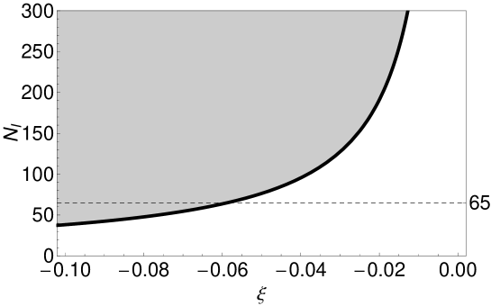
Figure 5: Parameter space of nonminimal coupling $\xi$, and the total number of e-foldings of inflation $N_{I}$. The bold curve corresponds to the condition $\rho_{Q}/\rho_{B}\!=\!1$ at the end of inflation ($H_{I}\!=\!10^{13}\,{\rm GeV}$), and the shaded region to situations when quantum backreaction starts to dominate even before the end of inflation. This part of parameter space is not examined in this work, but rather concentrate on the white region where quantum backreaction stays perturbative during inflation. The dashed line represents the requirement on the minimal duration of inflation. It follows that we restrict ourselves to considering $-0.05\lesssim\xi\leq 0$ in this work.

This implies for the number of e-foldings,

$$N_{I}\leq\frac{1}{8|\xi|}\ln\biggl{[}4\pi\Bigl{(}\frac{E_{P}}{\hbar H_{I}}\Bigr{)}^{2}\biggr{]}\,,$$ (155)

where the dimensionful units were restored, and $E_{P}\!=\!(\hbar c^{5}/G_{\!N})^{1/2}$ is the Planck energy, and the inflationary Hubble scale is taken to be $\hbar H_{I}\!\sim\!10^{13}\,{\rm GeV}$.

Although strong backreaction in inflation would be very interesting to study in its own right (especially since its energy density has a negative sign which would work towards slowing down inflation), here we restrict ourself to studying just the DE scenarios, for which we assume small backreaction at the end of inflation.

VII.2 Radiation era

Some time after the transition to the radiation period the hierarchy of scales $k_{0}\!\ll\!\mathcal{H}\!\ll\!\mathcal{H}_{1}$ is reached (together with the assumed $(ma)^{2}/\mathcal{H}^{2}\!\ll\!1$). The relevant contribution to integrals (35) is

$$\mathcal{I}_{n}\approx\int\limits_{k_{0}}^{\mu}\!dk\,k^{2+2n}Z_{\text{Bog.}}(k,\eta)\,,$$ (156)

as was established in subsection V.2.1, with

$$k_{0}\!\ll\!\mathcal{H}\!\ll\!\mu\!\ll\!\mathcal{H}_{1}\,,$$ (157)

and the integrand, as defined in (58), is

$$Z_{\text{Bog.}}(k,\eta)=2|\beta_{R}(k)|^{2}|u_{R}(k,\eta)|^{2}+\alpha_{R}(k)\beta^{*}(k)u_{R}^{2}(k,\eta)+\alpha_{R}^{*}(k)\beta_{R}(k)[u_{R}^{2}(k,\eta)]^{*}\,.$$ (158)

The Bogolyubov coefficients in this integrand are determined by the fast transition from the inflationary period to the radiation one. For the scales integrated over in (156) they are well approximated by the sudden transition ones (52) and (53),

$$\alpha_{R}(k)={} -i\Bigl{[}u_{I}(k,\eta_{1})u_{R}^{\prime*}(k,\eta_{1})-u_{I}^{\prime}(k,\eta_{1})u_{R}^{*}(k,\eta_{1})\Bigr{]}\,,$$ (159)

$$\beta_{R}(k)={} i\Bigl{[}u_{I}(k,\eta_{1})u_{R}^{\prime}(k,\eta_{1})-u_{I}^{\prime}(k,\eta_{1})u_{R}(k,\eta_{1})\Bigr{]}\,.$$ (160)

The inflationary CTBD mode function in Bogolyubov coefficients above is given by (73), and the radiation CTBD mode function by (115). For the range of integration in (156), the mode functions inside of Bogolyubov coefficients are in fact very well described by the small momentum limit (on top of small mass limit). We use this to simplify the integrand before integration.

Using the IR expansion (75) for the inflationary CTBD mode function, it follows that

$$u_{I}^{\prime}(k,\eta_{1})\approx\bigl{(}\nu_{I}\!-\!\tfrac{1}{2}\bigr{)}\mathcal{H}_{1}u_{I}(k,\eta_{1})\,,$$ (161)

and the Bogolyubov coefficients simplify to

$$\alpha_{R}(k)\approx{} -\bigl{|}u_{I}(k,\eta_{1})\bigr{|}\Bigl{[}u_{R}^{\prime*}(k,\eta_{1})-\bigl{(}\nu_{I}\!-\!\tfrac{1}{2}\bigr{)}\mathcal{H}_{1}u_{R}^{*}(k,\eta_{1})\Bigr{]}\equiv-\bigl{|}u_{I}(k,\eta_{1})\bigr{|}\widetilde{\beta}_{R}^{*}(k)\,,$$ (162)

$$\beta_{R}(k)\approx{} \bigl{|}u_{I}(k,\eta_{1})\bigr{|}\Bigl{[}u_{R}^{\prime}(k,\eta_{1})-\bigl{(}\nu_{I}\!-\!\tfrac{1}{2}\bigr{)}\mathcal{H}_{1}u_{R}(k,\eta_{1})\Bigr{]}\equiv\bigl{|}u_{I}(k,\eta_{1})\bigr{|}\widetilde{\beta}_{R}(k)\,,$$ (163)

and to leading order satisfy

$$\alpha_{R}(k)\approx-\beta_{R}^{*}(k)\,,$$ (164)

which implies the following simplification for the integrand (158),

$$Z_{\text{Bog.}}(k,\eta)\approx 4\bigl{|}u_{I}(k,\eta_{1})\bigr{|}^{2}\biggl{\{}\Im\Bigl{[}\widetilde{\beta}_{R}^{*}\,u_{R}(k,\eta)\Bigr{]}\biggr{\}}^{2}\,.$$ (165)

This integrand is further simplified by considering the small mass limit $ma/\mathcal{H}\!\ll\!1$, using the approximate mode functions (113) and (114),

$$\Im\Bigl{[}\widetilde{\beta}_{R}^{*}(k)u_{R}(k,\eta)\Bigr{]}\approx{} \Im\Bigl{[}A_{R}^{*}(k,m)B_{R}(k,m)\Bigr{]}\times\biggl{\{}v_{R2}^{\prime}(k,\eta_{1})v_{R1}(k,\eta)-v_{R1}^{\prime}(k,\eta_{1})v_{R2}(k,\eta)$$

$$-\bigl{(}\nu_{I}\!-\!\tfrac{1}{2}\bigr{)}\mathcal{H}_{1}\Bigl{[}v_{R2}(k,\eta_{1})v_{R1}(k,\eta)-v_{R1}(k,\eta_{1})v_{R2}(k,\eta)\Bigr{]}\biggr{\}}$$

$$={} \frac{1}{2}\biggl{\{}v_{R2}^{\prime}(k,\eta_{1})v_{R1}(k,\eta)-v_{R1}^{\prime}(k,\eta_{1})v_{R2}(k,\eta)$$

$$-\bigl{(}\nu_{I}\!-\!\tfrac{1}{2}\bigr{)}\mathcal{H}_{1}\Bigl{[}v_{R2}(k,\eta_{1})v_{R1}(k,\eta)-v_{R1}(k,\eta_{1})v_{R2}(k,\eta)\Bigr{]}\biggr{\}}\,,$$ (166)

where the property (116) was used, and it is the only place where we need to refer to coefficients $A_{R}$ and $B_{R}$, no matter how complicated they may be. Furthermore, we may expand this expression to leading order in $\mathcal{H}_{1}$ because of hierarchy (157),

$$\Im\Bigl{[}\widetilde{\beta}_{R}^{*}(k)u_{R}(k,\eta)\Bigr{]}\approx{} -\frac{1}{2}\bigl{(}\nu_{I}\!-\!\tfrac{1}{2}\bigr{)}\Biggl{\{}\frac{\mathcal{H}}{k}\sin\Bigl{(}\frac{k}{\mathcal{H}}\Bigr{)}+\Bigl{(}\frac{ma}{\mathcal{H}}\Bigr{)}^{\!2}\Bigl{(}\frac{\mathcal{H}}{k}\Bigr{)}^{\!2}\biggl{[}-\Bigl{(}1\!-\!\frac{\mathcal{H}^{2}}{k^{2}}\Bigr{)}\frac{\mathcal{H}}{4k}\sin\Bigl{(}\frac{k}{\mathcal{H}}\Bigr{)}$$

$$+\frac{1}{6}\Bigl{(}1\!-\!\frac{3\mathcal{H}^{2}}{2k^{2}}\Bigr{)}\cos\Bigl{(}\frac{k}{\mathcal{H}}\Bigr{)}\biggr{]}+\mathcal{O}\Bigl{(}\frac{ma}{\mathcal{H}}\Bigr{)}^{\!4}\Biggr{\}}\Bigl{(}\frac{\mathcal{H}_{1}}{\mathcal{H}}\Bigr{)}\Bigl{[}1+\mathcal{O}\Bigl{(}\frac{\mathcal{H}}{\mathcal{H}_{1}}\Bigr{)}\Bigr{]}\,,$$ (167)

so that now, after plugging in (73), the full integrand is well approximated by

$$Z_{\text{Bog.}}\approx{} \frac{4^{\nu_{I}-1}}{\pi}\Gamma^{2}(\nu_{I})\bigl{(}\nu_{I}\!-\!\tfrac{1}{2}\bigr{)}^{2}\Bigl{(}\frac{\mathcal{H}_{1}}{\mathcal{H}}\Bigr{)}^{\!2}\mathcal{H}_{1}^{2\nu_{I}-1}k^{-2\nu_{I}}\Biggl{\{}\frac{\mathcal{H}^{2}}{k^{2}}\sin^{2}\Bigl{(}\frac{k}{\mathcal{H}}\Bigr{)}$$

$$+\Bigl{(}\frac{ma}{\mathcal{H}}\Bigr{)}^{\!2}\times\frac{2\mathcal{H}^{3}}{k^{3}}\sin\Bigl{(}\frac{k}{\mathcal{H}}\Bigr{)}\biggl{[}-\Bigl{(}1\!-\!\frac{\mathcal{H}^{2}}{k^{2}}\Bigr{)}\frac{\mathcal{H}}{4k}\sin\Bigl{(}\frac{k}{\mathcal{H}}\Bigr{)}+\frac{1}{6}\Bigl{(}1\!-\!\frac{3\mathcal{H}^{2}}{2k^{2}}\Bigr{)}\cos\Bigl{(}\frac{k}{\mathcal{H}}\Bigr{)}\biggr{]}\Biggr{\}}\,.$$ (168)

Finally, we can perform the integrals (156) using this approximated integrand. The result we expand according to the hierarchy (157),

$$\mathcal{I}_{0}\approx{} \frac{\Gamma^{2}(\nu_{I})}{2^{3-2\nu_{I}}\pi}\bigl{(}\nu_{I}\!-\!\tfrac{1}{2}\bigr{)}^{2}\Biggl{\{}\frac{1}{\left(\nu_{I}\!-\!\frac{3}{2}\right)}\biggl{[}1-\frac{1}{10}\Bigl{(}\frac{ma}{\mathcal{H}}\Bigr{)}^{\!2}+\mathcal{O}\Bigl{(}\frac{ma}{\mathcal{H}}\Bigr{)}^{\!4}\biggr{]}\Bigl{(}\frac{\mathcal{H}_{0}}{\mathcal{H}}\Bigr{)}^{\!3-2\nu_{I}}\Bigl{[}1+\mathcal{O}\Bigl{(}\frac{\mathcal{H}_{0}}{\mathcal{H}}\Bigr{)}^{\!2}\Bigr{]}$$

$$-\frac{\Gamma(1\!-\!2\nu_{I})}{2^{1-2\nu_{I}}}\sin(\pi\nu_{I})\biggl{[}1-\frac{8\Gamma(-3\!-\!2\nu_{I})}{3\Gamma(1\!-\!2\nu_{I})}\bigl{(}\nu_{I}\!-\!\tfrac{1}{2}\bigr{)}(2\nu_{I}^{2}\!+\!4\nu_{I}\!+\!3)\Bigl{(}\frac{ma}{\mathcal{H}}\Bigr{)}^{\!2}+\mathcal{O}\Bigl{(}\frac{ma}{\mathcal{H}}\Bigr{)}^{\!4}\biggr{]}$$

$$-\frac{1}{2\left(\nu_{I}\!-\!\frac{1}{2}\right)}\Bigl{(}\frac{\mathcal{H}}{\mu}\Bigr{)}^{2\nu_{I}-1}\Bigl{[}1+\mathcal{O}\Bigl{(}\frac{\mathcal{H}}{\mu}\Bigr{)}^{\!2}\Bigr{]}\Biggr{\}}\mathcal{H}^{2}\Bigl{(}\frac{\mathcal{H}_{1}}{\mathcal{H}}\Bigr{)}^{\!2\nu_{I}+1}\Bigl{[}1+\mathcal{O}\Bigl{(}\frac{\mathcal{H}}{\mathcal{H}_{1}}\Bigr{)}\Bigr{]}\,,$$ (169)

$$\mathcal{I}_{1}\approx{} \frac{\Gamma^{2}(\nu_{I})}{2^{3-2\nu_{I}}\pi}\bigl{(}\nu_{I}\!-\!\tfrac{1}{2}\bigr{)}^{2}\Biggl{\{}\frac{1}{\left(\nu_{I}\!-\!\frac{5}{2}\right)}\biggl{[}1-\frac{1}{10}\Bigl{(}\frac{ma}{\mathcal{H}}\Bigr{)}^{\!2}+\mathcal{O}\Bigl{(}\frac{ma}{\mathcal{H}}\Bigr{)}^{\!4}\biggr{]}\Bigl{(}\frac{\mathcal{H}_{0}}{\mathcal{H}}\Bigr{)}^{\!5-2\nu_{I}}\Bigl{[}1+\mathcal{O}\Bigl{(}\frac{\mathcal{H}_{0}}{\mathcal{H}}\Bigr{)}^{\!2}\Bigr{]}$$

$$+\frac{\Gamma(3\!-\!2\nu_{I})}{2^{3-2\nu_{I}}}\sin(\pi\nu_{I})\biggl{[}1-\frac{8\Gamma(-1\!-\!2\nu_{I})}{3\Gamma(3\!-\!2\nu_{I})}\bigl{(}\nu_{I}\!-\!\tfrac{3}{2}\bigr{)}(2\nu_{I}^{2}\!+\!1)\Bigl{(}\frac{ma}{\mathcal{H}}\Bigr{)}^{\!2}+\mathcal{O}\Bigl{(}\frac{ma}{\mathcal{H}}\Bigr{)}^{\!4}\biggr{]}$$

$$-\frac{1}{2\left(\nu_{I}\!-\!\frac{3}{2}\right)}\Bigl{(}\frac{\mathcal{H}}{\mu}\Bigr{)}^{2\nu_{I}-3}\Bigl{[}1+\mathcal{O}\Bigl{(}\frac{\mathcal{H}}{\mu}\Bigr{)}^{\!2}\Bigr{]}\Biggr{\}}\mathcal{H}^{4}\Bigl{(}\frac{\mathcal{H}_{1}}{\mathcal{H}}\Bigr{)}^{\!2\nu_{I}+1}\Bigl{[}1+\mathcal{O}\Bigl{(}\frac{\mathcal{H}}{\mathcal{H}_{1}}\Bigr{)}\Bigr{]}\,.$$ (170)

Then plugging them into (33) and (34) gives the backreaction energy density and pressure (in the small mass limit),

$$\rho_{Q}\approx{} \frac{\Gamma(\nu_{I})H_{I}^{4}}{2^{5-2\nu_{I}}\pi^{3}}\bigl{(}\nu_{I}\!-\!\tfrac{1}{2}\bigr{)}e^{(2\nu_{I}\!-\!3)N_{I}}\Biggl{\{}\frac{\left(\nu_{I}\!-\!\frac{1}{2}\right)\Gamma(\nu_{I})}{\left(\nu_{I}\!-\!\frac{3}{2}\right)}\,\biggl{[}6\xi\Bigl{(}\frac{a_{1}}{a}\Bigr{)}^{\!4}+(1\!-\!3\xi)\Bigl{(}\frac{m}{H_{I}}\Bigr{)}^{\!2}\biggr{]}$$

$$\hskip 14.22636pt-\frac{\left(\nu_{I}\!-\!\frac{1}{2}\right)\Gamma(\nu_{I})}{\left(\nu_{I}\!-\!\frac{3}{2}\right)}\Bigl{(}\frac{\mathcal{H}_{0}}{\mu}\Bigr{)}^{\!2\nu_{I}-3}\Bigl{(}\frac{a_{1}}{a}\Bigr{)}^{\!4}-\sqrt{\pi}(\nu_{I}\!-\!1)\Gamma\bigl{(}\tfrac{3}{2}\!-\!\nu_{I}\bigr{)}\biggl{[}(1\!-\!6\xi)\Bigl{(}\frac{a_{1}}{a}\Bigr{)}^{\!4}$$

$$\hskip 14.22636pt-\frac{(1\!-\!6\xi)\left(\nu_{I}\!-\!\frac{3}{2}\right)+3\nu_{I}\left(\nu_{I}\!+\!\frac{3}{2}\right)+2(1\!-\!6\xi)\nu_{I}^{2}\left(\nu_{I}\!+\!\frac{3}{2}\right)}{6\nu_{I}(\nu_{I}\!-\!1)\left(\nu_{I}\!+\!\frac{1}{2}\right)\left(\nu_{I}\!+\!\frac{3}{2}\right)}\Bigl{(}\frac{m}{H_{I}}\Bigr{)}^{\!2}\biggr{]}\Bigl{(}\frac{\mathcal{H}_{0}}{\mathcal{H}}\Bigr{)}^{\!3\!-\!2\nu_{I}}\Biggr{\}}\,,$$ (171)

$$p_{Q}\approx{} \frac{\Gamma(\nu_{I})H_{I}^{4}}{2^{5-2\nu_{I}}\pi^{3}}\bigl{(}\nu_{I}\!-\!\tfrac{1}{2}\bigr{)}e^{(2\nu_{I}\!-\!3)N_{I}}\Biggl{\{}\frac{\left(\nu_{I}\!-\!\frac{1}{2}\right)\Gamma(\nu_{I})}{\left(\nu_{I}\!-\!\frac{3}{2}\right)}\,\biggl{[}2\xi\Bigl{(}\frac{a_{1}}{a}\Bigr{)}^{\!4}-(1\!-\!3\xi)\Bigl{(}\frac{m}{H_{I}}\Bigr{)}^{\!2}\biggr{]}$$

$$\hskip 14.22636pt-\frac{\left(\nu_{I}\!-\!\frac{1}{2}\right)\Gamma(\nu_{I})}{3\left(\nu_{I}\!-\!\frac{3}{2}\right)}\Bigl{(}\frac{\mathcal{H}_{0}}{\mu}\Bigr{)}^{\!2\nu_{I}-3}\Bigl{(}\frac{a_{1}}{a}\Bigr{)}^{\!4}+\frac{2\sqrt{\pi}}{3}(\nu_{I}\!-\!1)\Gamma\bigl{(}\tfrac{3}{2}\!-\!\nu_{I}\bigr{)}\biggl{[}(1\!-\!6\xi)(\nu_{I}\!-\!2)\Bigl{(}\frac{a_{1}}{a}\Bigr{)}^{\!4}$$

$$\hskip 14.22636pt-\frac{(1\!-\!6\xi)\left(\nu_{I}\!-\!\frac{3}{2}\right)+3\nu_{I}\left(\nu_{I}\!+\!\frac{3}{2}\right)+2(1\!-\!6\xi)\nu_{I}^{2}\left(\nu_{I}\!+\!\frac{3}{2}\right)}{6(\nu_{I}\!-\!1)\left(\nu_{I}\!+\!\frac{1}{2}\right)\left(\nu_{I}\!+\!\frac{3}{2}\right)}\Bigl{(}\frac{m}{H_{I}}\Bigr{)}^{\!2}\biggr{]}\Bigl{(}\frac{\mathcal{H}_{0}}{\mathcal{H}}\Bigr{)}^{\!3\!-\!2\nu_{I}}\Biggr{\}}\,.$$ (172)

We have given some parts of the expressions above in terms of physical quantities for the sake of clarity. The comment of the dependence on the arbitrary cutoff $\mu$ is warranted. It is bound to cancel with the same contribution from the remaining part of integration interval, and it does not contribute to the full result. The reason we kept it explicitly is because we want to take the minimally coupled limit, which we do and discuss in the next subsection.

VII.2.1 Minimally coupled limit

The minimally coupled limit consists in taking $\xi\!=\!0$, and then expanding $\nu_{I}$, defined in (74), for small mass in (171) and (172),

$$\rho_{Q}\approx{} \frac{3H_{I}^{4}}{16\pi^{2}}\biggl{[}1-e^{-\frac{2}{3}\frac{m^{2}}{H_{I}^{2}}N_{I}}\biggr{]}+\frac{H_{I}^{4}}{8\pi^{2}}\biggl{[}\ln\Bigl{(}\frac{a}{a_{1}}\Bigr{)}-\frac{1}{2}+\ln\Bigl{(}\frac{2\mu}{a_{1}H_{I}}\Bigr{)}+\gamma_{E}\biggr{]}\Bigl{(}\frac{a_{1}}{a}\Bigr{)}^{4}\,,$$ (173)

$$p_{Q}\approx{} -\frac{3H_{I}^{4}}{16\pi^{2}}\biggl{[}1-e^{-\frac{2}{3}\frac{m^{2}}{H_{I}^{2}}N_{I}}\biggr{]}+\frac{H_{I}^{4}}{24\pi^{2}}\biggl{[}\ln\Bigl{(}\frac{a}{a_{1}}\Bigr{)}-\frac{3}{2}+\ln\Bigl{(}\frac{2\mu}{a_{1}H_{I}}\Bigr{)}+\gamma_{E}\biggr{]}\Bigl{(}\frac{a_{1}}{a}\Bigr{)}^{4}\,.$$ (174)

Note that the dependence on $\mu$ has persisted in the final answer. This does not signal that the answer is wrong, but rather that the UV does not contribute a suppressed contribution. In the exactly massless limit of this result the first terms drop out from the energy density and pressure above, and what remains is exactly the result from Glavan:2013mra , where the massless minimally coupled case was studied from the start. What effectively cuts off the UV radiation-like contribution is the finite time of transition $\tau$ between the inflationary and radiation period.

We have assumed here that the radiation period does not last excessively long, more precisely,

$$N_{R}\ll\Bigl{(}\frac{m}{H_{I}}\Bigr{)}^{\!-2}\,,$$ (175)

where $N_{R}$ is the total number of e-foldings of radiation period, which will be satisfied by the requirements in the end. This first terms in (173) and (174) coincide with the ones computed in Aoki:2014dqa , since they derive from $m^{2}\langle\hat{\phi}^{2}\rangle$ term. Note that this term is not the dominant one for a very small mass.

VII.2.2 Limit $(m/H)^{2}\sim|\xi|\ll 1$

The leading order contribution in this limit is

$$\rho_{Q}\approx{} -\frac{3H_{I}^{4}}{32\pi^{2}}\,e^{8|\xi|N_{I}}\Biggl{[}\Bigl{(}\frac{a_{1}}{a}\Bigr{)}^{\!4}-\frac{1}{6|\xi|}\Bigl{(}\frac{m}{H_{I}}\Bigr{)}^{\!2}\Biggr{]}\,,$$ (176)

$$p_{Q}\approx{} -\frac{3H_{I}^{4}}{32\pi^{2}}\,e^{8|\xi|N_{I}}\Biggl{[}\frac{1}{3}\Bigl{(}\frac{a_{1}}{a}\Bigr{)}^{\!4}+\frac{1}{6|\xi|}\Bigl{(}\frac{m}{H_{I}}\Bigr{)}^{\!2}\Biggr{]}\,,$$ (177)

where we have assumed that the radiation period will not last longer (in e-foldings) than the inflationary period ($N_{I}\!>\!N_{R}\sim 60$), which will be true in the end for the ranges of nonminimal couplings of interest in this work. There are two qualitatively different contributions to the energy density and pressure above. The first contribution is radiation-like and it redshifts just as the background does. It is easy to see that if the constraint from Figure 5 is satisfied, this contribution will never dominate in radiation period.

The second contribution is of the CC type, and its energy density has a positive sign. For suitable choices of parameters one can get this contribution to be the dominant one in the backreaction during radiation period. And since it does not redshift away the ratio $\rho_{Q}/\rho_{B}$ grows, and it might grow to order one for suitable masses and small enough nonminimal couplings. But we are not interested in this scenario happening in radiation period. What we are interested in is realizing it in matter period, which we turn to next. During radiation period we require the CC-type contribution to be negligible, in which case (176) and (177) reduce to the massless limit of Glavan:2014uga ,

$$\rho_{Q}\approx-\frac{3H_{I}^{4}}{32\pi^{2}}\,e^{8|\xi|N_{I}}\Bigl{(}\frac{a_{1}}{a}\Bigr{)}^{\!4}\,,\qquad p_{Q}\approx\frac{1}{3}\rho_{Q}\,.$$ (178)

VII.3 Matter era

After the transition to the matter era, the following hierarchy of scales is reached (Fig. 2),

$$\mathcal{H}_{0}\ll\mathcal{H}\ll\mu\ll\mathcal{H}_{2}\ll\mathcal{H}_{1}\,,$$ (179)

where $\mu$ is a fiducial scale, introduced for the sake of isolating the relevant contribution to integrals (35),

$$\mathcal{I}_{n}\approx\int\limits_{\mathcal{H}_{0}}^{\mu}\!dk\,k^{2+2n}Z_{\text{Bog.}}(k,\eta)\,,$$ (180)

as discussed in Section V. The integrand here is

$$Z_{\text{Bog.}}=2\bigl{|}\beta_{M}(k)\bigr{|}^{2}\bigl{|}u_{M}(k,\eta)\bigr{|}^{2}+\alpha_{M}(k)\beta_{M}^{*}(k)u_{M}^{2}(k,\eta)+\alpha_{M}^{*}(k)\beta_{M}(k)[u_{M}^{2}(k,\eta)]^{*}\,,$$ (181)

where the Bogolyubov coefficients are well approximated by the sudden transition ones (52) and (53) determined by two fast transitions – from inflation to radiation, and from radiation to matter,

$$\alpha_{M}(k)={} -i\Bigl{[}\alpha_{R}(k)u_{R}(k,\eta_{2})+\beta_{R}(k)u_{R}^{*}(k,\eta_{2})\Bigr{]}u_{M}^{\prime*}(k,\eta_{2})$$

$$\hskip 56.9055pt+i\Bigl{[}\alpha_{R}(k)u_{R}^{\prime}(k,\eta_{2})+\beta_{R}(k)u_{R}^{\prime*}(k,\eta_{2})\Bigr{]}u_{M}^{*}(k,\eta_{2})\,,$$ (182)

$$\beta_{M}(k)={} i\Bigl{[}\alpha_{R}(k)u_{R}(k,\eta_{2})+\beta_{R}(k)u_{R}^{*}(k,\eta_{2})\Bigr{]}u_{M}^{\prime}(k,\eta_{2})$$

$$\hskip 56.9055pt+i\Bigl{[}\alpha_{R}(k)u_{R}^{\prime}(k,\eta_{2})+\beta_{R}(k)u_{R}^{\prime*}(k,\eta_{2})\Bigr{]}u_{M}(k,\eta_{2})\,.$$ (183)

Bogolyubov coefficients in radiation period $\alpha_{R}$ and $\beta_{R}$, appearing in the expression above, were already approximated in the previous subsection, where it was found that $\alpha_{R}\!\approx\!-\beta_{R}^{*}$. Applying this here gives

$$\alpha_{M}(k)\approx{} -2\Im\Bigl{[}\beta_{R}^{*}(k)u_{R}(k,\eta_{2})\Bigr{]}u_{M}^{\prime*}(k,\eta_{2})+2\Im\Bigl{[}\beta_{R}^{*}(k)u_{R}^{\prime}(k,\eta_{2})\Bigr{]}u_{M}^{*}(k,\eta_{2})\,,$$ (184)

$$\beta_{M}(k)\approx{} 2\Im\Bigl{[}\beta_{R}^{*}(k)u_{R}(k,\eta_{2})\Bigr{]}u_{M}^{\prime}(k,\eta_{2})-2\Im\Bigl{[}\beta_{R}^{*}(k)u_{R}^{\prime}(k,\eta_{2})\Bigr{]}u_{M}(k,\eta_{2})\,,$$ (185)

from where we see that again

$$\alpha_{M}(k)\approx-\beta_{M}^{*}(k)\,.$$ (186)

Now the integrand (181) simplifies to

$$Z_{\text{Bog.}}(k,\eta)\approx 4\biggl{\{}\Im\Bigl{[}\beta_{M}^{*}(k)u_{M}(k,\eta)\Bigr{]}\biggr{\}}^{2}\,.$$ (187)

which we can write out as

$$\Im\Bigl{[}\beta_{M}^{*}(k)u_{M}(k,\eta)\Bigr{]}={} 2\Im\Bigl{[}\beta_{R}^{*}(k)u_{R}(k,\eta_{2})\Bigr{]}\Im\Bigl{[}u_{M}^{\prime*}(k,\eta_{2})u_{M}(k,\eta)\Bigr{]}$$

$$-2\Im\Bigl{[}\beta_{R}^{*}(k)u_{R}^{\prime}(k,\eta_{2})\Bigr{]}\Im\Bigl{[}u_{M}^{*}(k,\eta_{2})u_{M}(k,\eta)\Bigr{]}\,.$$ (188)

Part of this integrand was already approximated in (168). Because of the hierarchy of scales (179) in matter period, we may expand this further in the IR limit,

$$\Im\Bigl{[}\beta_{R}^{*}(k)u_{R}(k,\eta_{2})\Bigr{]}\approx{} -\frac{2^{\nu_{I}-2}}{\sqrt{\pi}}\Gamma(\nu_{I})\bigl{(}\nu_{I}\!-\!\tfrac{1}{2}\bigr{)}\mathcal{H}_{1}^{\nu_{I}+1/2}\mathcal{H}_{2}^{-1}k^{-\nu_{I}}\biggl{[}1\!-\!\frac{1}{20}\Bigl{(}\frac{ma_{2}}{\mathcal{H}_{2}}\Bigr{)}^{\!2}\biggr{]}\,,$$ (189)

$$\Im\Bigl{[}\beta_{R}^{*}(k)u_{R}^{\prime}(k,\eta_{2})\Bigr{]}\approx{} -\frac{2^{\nu_{I}-2}}{\sqrt{\pi}}\Gamma(\nu_{I})\bigl{(}\nu_{I}\!-\!\tfrac{1}{2}\bigr{)}\mathcal{H}_{1}^{\nu_{I}+1/2}k^{-\nu_{I}}\biggl{[}1\!-\!\frac{1}{8}\Bigl{(}\frac{ma_{2}}{\mathcal{H}_{2}}\Bigr{)}^{\!2}\biggr{]}\,.$$ (190)

In the remaining part of the integrand we first use the property (142) to express it solely in terms of mode functions (139) and (140),

$$\Im\Bigl{[}u_{M}^{\prime*}(k,\eta_{2})u_{M}(k,\eta)\Bigr{]}={} \Im\Bigl{[}A_{M}^{*}(k,m)B_{M}(k,m)\Bigr{]}\!\times\!\Bigl{[}v_{M1}(k,\eta_{1})v_{M2}(k,\eta)-v_{M2}(k,\eta_{2})v_{M1}(k,\eta)\Bigr{]}$$

$$={} \frac{1}{2\nu}\Bigl{[}v_{M1}(k,\eta_{1})v_{M2}(k,\eta)-v_{M2}(k,\eta_{2})v_{M1}(k,\eta)\Bigr{]}\,,$$ (191)

and then we use the hierarchy (179) to simplify it further by expanding it to leading order in $\mathcal{H}_{2}$,

$$\Im\Bigl{[}u_{M}^{*}(k,\eta_{2})u_{M}(k,\eta)\Bigr{]}\approx\frac{\Gamma(\nu)}{2}\mathcal{H}_{2}^{-1/2+\nu}\mathcal{H}^{-1/2}k^{-\nu}$$

$$\hskip 28.45274pt\times\Biggl{\{}J_{\nu}\Bigl{(}\frac{2k}{\mathcal{H}}\Bigr{)}+\Bigl{(}\frac{ma}{\mathcal{H}}\Bigr{)}^{2}\times\frac{\mathcal{H}}{30k}\biggl{[}\Bigl{(}-6\!+\!(1\!-\!\nu)(2\!-\!\nu)\frac{\mathcal{H}^{2}}{k^{2}}\Bigr{)}J_{1+\nu}\Bigl{(}\frac{2k}{\mathcal{H}}\Bigr{)}$$

$$\hskip 150.79968pt+(2\!-\!\nu)\Bigl{(}3\!-\!(1\!-\!\nu)(2\!+\!\nu)\frac{\mathcal{H}^{2}}{k^{2}}\Bigr{)}\frac{\mathcal{H}}{k}J_{2+\nu}\Bigl{(}\frac{2k}{\mathcal{H}}\Bigr{)}\biggr{]}\Biggr{\}}\,,$$ (192)

$$\Im\Bigl{[}u_{M}^{\prime*}(k,\eta_{2})u_{M}(k,\eta)\Bigr{]}\approx-\frac{1}{2}\bigl{(}\nu\!-\!\tfrac{1}{2}\bigr{)}\mathcal{H}_{2}\times\Im\Bigl{[}u_{M}^{*}(k,\eta_{2})u_{M}(k,\eta)\Bigr{]}\,.$$ (193)

The full integrand is now given approximately as

$$Z_{\text{Bog.}}(k,\eta)\approx{} \frac{2^{2\nu_{I}-2}}{\pi}\Gamma^{2}(\nu_{I})\bigl{(}\nu_{I}\!-\!\tfrac{1}{2}\bigr{)}^{2}\bigl{(}\nu\!+\!\tfrac{3}{2}\bigr{)}^{2}\mathcal{H}_{1}^{2\nu_{I}-1}k^{-2\nu_{I}}\biggl{\{}\Im\Bigl{[}u_{M}^{*}(k,\eta_{2})u_{M}(k,\eta)\Bigr{]}\biggr{\}}^{2}$$

$$={} \frac{2^{2\nu_{I}-4}}{\pi}\Gamma^{2}(\nu_{I})\Gamma^{2}(\nu)\bigl{(}\nu_{I}\!-\!\tfrac{1}{2}\bigr{)}^{2}\bigl{(}\nu\!+\!\tfrac{3}{2}\bigr{)}^{2}\mathcal{H}_{1}^{2\nu_{I}+1}\mathcal{H}_{2}^{2\nu-1}\mathcal{H}^{-1}k^{-2\nu_{I}-2\nu}$$

$$\times\Biggl{\{}J_{\nu}^{2}\Bigl{(}\frac{2k}{\mathcal{H}}\Bigr{)}+\Bigl{(}\frac{ma}{\mathcal{H}}\Bigr{)}^{2}\times\frac{\mathcal{H}}{15k}J_{\nu}\Bigl{(}\frac{2k}{\mathcal{H}}\Bigr{)}\biggl{[}\Bigl{(}-6\!+\!(1\!-\!\nu)(2\!-\!\nu)\frac{\mathcal{H}^{2}}{k^{2}}\Bigr{)}J_{1+\nu}\Bigl{(}\frac{2k}{\mathcal{H}}\Bigr{)}$$

$$\hskip 113.81102pt+(2\!-\!\nu)\Bigl{(}3\!-\!(1\!-\!\nu)(2\!+\!\nu)\frac{\mathcal{H}^{2}}{k^{2}}\Bigr{)}\frac{\mathcal{H}}{k}J_{2+\nu}\Bigl{(}\frac{2k}{\mathcal{H}}\Bigr{)}\biggr{]}\Biggr{\}}\,.$$ (194)

Given the approximation (194), we can now perform integrals (35), and expand the result according to the hierarchy (179),

$$\mathcal{I}_{0}\approx{} \frac{\Gamma^{2}(\nu_{I})\Gamma^{2}(\nu)}{2^{5-2\nu_{I}}\pi}\bigl{(}\nu_{I}\!-\!\tfrac{1}{2}\bigr{)}^{2}\bigl{(}\nu\!+\!\tfrac{3}{2}\bigr{)}^{2}\times\Biggl{\{}\frac{1}{\left(\nu_{I}\!-\!\tfrac{3}{2}\right)\Gamma^{2}(1\!+\!\nu)}\Bigl{(}\frac{\mathcal{H}_{1}}{\mathcal{H}_{0}}\Bigr{)}^{2\nu_{I}-3}\biggl{[}1-\frac{2}{3(3\!+\!\nu)}\Bigl{(}\frac{ma}{\mathcal{H}}\Bigr{)}^{\!2}\biggr{]}$$

$$\hskip 28.45274pt-\frac{2^{-3+2\nu+2\nu_{I}}\Gamma\left(\frac{3}{2}\!-\!\nu_{I}\right)\Gamma(\nu_{I}\!+\!\nu\!-\!1)}{\sqrt{\pi}\,\Gamma(\nu_{I}\!+\!\nu\!-\!\frac{1}{2})\Gamma(\nu_{I}\!+\!2\nu\!-\!\frac{1}{2})}\Bigl{(}\frac{\mathcal{H}_{1}}{\mathcal{H}_{2}}\Bigr{)}^{\!2\nu_{I}-3}\Bigl{(}\frac{\mathcal{H}_{2}}{\mathcal{H}}\Bigr{)}^{\!2\nu_{I}-3}\Bigl{[}1+\mathcal{O}\Bigl{(}\frac{ma}{\mathcal{H}}\Bigr{)}^{\!2}\Bigr{]}\Biggr{\}}$$

$$\times\Bigl{(}\frac{\mathcal{H}_{1}}{\mathcal{H}_{2}}\Bigr{)}^{\!4}\Bigl{(}\frac{\mathcal{H}_{2}}{\mathcal{H}}\Bigr{)}^{2\nu_{I}-3}\mathcal{H}^{2}\,,$$ (195)

$$\mathcal{I}_{1}\approx{} \frac{\Gamma^{2}(\nu_{I})\Gamma^{2}(\nu)}{2^{5-2\nu_{I}}\pi}\bigl{(}\nu_{I}\!-\!\tfrac{1}{2}\bigr{)}^{2}\bigl{(}\nu\!+\!\tfrac{3}{2}\bigr{)}^{2}\times\Biggl{\{}\frac{1}{\left(\nu_{I}\!-\!\tfrac{5}{2}\right)\Gamma^{2}(1\!+\!\nu)}\Bigl{(}\frac{\mathcal{H}_{1}}{\mathcal{H}_{0}}\Bigr{)}^{2\nu_{I}-3}\mathcal{H}_{0}^{2}\biggl{[}1-\frac{2}{3(3\!+\!\nu)}\Bigl{(}\frac{ma}{\mathcal{H}}\Bigr{)}^{\!2}\biggr{]}$$

$$\hskip 28.45274pt+\frac{2^{-5+2\nu+2\nu_{I}}\Gamma\left(\frac{5}{2}\!-\!\nu_{I}\right)\Gamma(\nu_{I}\!+\!\nu\!-\!2)}{\sqrt{\pi}\,\Gamma(\nu_{I}\!+\!\nu\!-\!\frac{3}{2})\Gamma(\nu_{I}\!+\!2\nu\!-\!\frac{3}{2})}\Bigl{(}\frac{\mathcal{H}_{1}}{\mathcal{H}_{2}}\Bigr{)}^{\!2\nu_{I}-3}\Bigl{(}\frac{\mathcal{H}_{2}}{\mathcal{H}}\Bigr{)}^{\!2\nu_{I}-3}\mathcal{H}^{2}\Bigl{[}1+\mathcal{O}\Bigl{(}\frac{ma}{\mathcal{H}}\Bigr{)}^{\!2}\Bigr{]}\Biggr{\}}$$

$$\times\Bigl{(}\frac{\mathcal{H}_{1}}{\mathcal{H}_{2}}\Bigr{)}^{\!4}\Bigl{(}\frac{\mathcal{H}_{2}}{\mathcal{H}}\Bigr{)}^{2\nu_{I}-3}\mathcal{H}^{2}\,.$$ (196)

Plugging these two integrals into (33) and (34) yields the backreaction energy density and pressure in matter era,

$$\rho_{Q}\approx{} \frac{\Gamma^{2}(\nu_{I})H_{I}^{4}}{2^{5-2\nu_{I}}}\bigl{(}\nu_{I}\!-\!\tfrac{1}{2}\bigr{)}^{2}\bigl{(}\nu\!+\!\tfrac{3}{2}\bigr{)}^{2}e^{(2\nu_{I}-3)N_{I}}$$

$$\Biggl{\{}\biggl{[}-\frac{\left(\nu\!-\!\frac{3}{2}\right)\left(\nu\!+\!\frac{1}{2}\right)}{8\nu(\nu_{I}\!-\!\frac{3}{2})}\,e^{-4N_{R}}\Bigl{(}\frac{a_{2}}{a}\Bigr{)}^{\!3}+\frac{\left(\nu^{2}\!-\!\nu\!+\!\frac{9}{4}\right)}{12\nu^{2}\left(\nu_{I}\!-\!\frac{3}{2}\right)}\Bigl{(}\frac{m}{H_{I}}\Bigr{)}^{\!2}\biggr{]}\Bigl{(}\frac{a_{2}}{a}\Bigr{)}^{\frac{3}{2}-\nu}$$

$$-\frac{(1\!-\!6\xi)(\nu_{I}\!+\!\nu\!-\!3)\,\Gamma\!\left(\frac{3}{2}\!-\!\nu_{I}\right)\Gamma^{2}(\nu)\,\Gamma(2\nu_{I}\!+\!2\nu\!-\!4)}{\Gamma^{2}\!\left(\nu_{I}\!+\!\nu\!-\!\frac{3}{2}\right)\Gamma\!\left(\nu_{I}\!+\!2\nu\!-\!\frac{1}{2}\right)}\,e^{-4N_{R}}\Bigl{(}\frac{a_{2}}{a}\Bigr{)}^{\!\frac{9}{2}-\nu}\Bigl{(}\frac{\mathcal{H}_{0}}{\mathcal{H}}\Bigr{)}^{2\nu_{I}-3}\Biggr{\}}\,,$$ (197)

$$p_{Q}\approx{} \frac{\Gamma^{2}(\nu_{I})H_{I}^{4}}{2^{5-2\nu_{I}}}\bigl{(}\nu_{I}\!-\!\tfrac{1}{2}\bigr{)}^{2}\bigl{(}\nu\!+\!\tfrac{3}{2}\bigr{)}^{2}e^{(2\nu_{I}-3)N_{I}}$$

$$\Biggl{\{}\biggl{[}\frac{\left(\nu\!-\!\frac{3}{2}\right)^{2}\left(\nu\!+\!\frac{1}{2}\right)}{24\nu(\nu_{I}\!-\!\frac{3}{2})}\,e^{-4N_{R}}\Bigl{(}\frac{a_{2}}{a}\Bigr{)}^{\!3}-\frac{\left(\nu\!+\!\frac{3}{2}\right)\left(\nu^{2}\!-\!\nu\!+\!\frac{9}{4}\right)}{36\nu^{2}\left(\nu_{I}\!-\!\frac{3}{2}\right)}\Bigl{(}\frac{m}{H_{I}}\Bigr{)}^{\!2}\biggr{]}\Bigl{(}\frac{a_{2}}{a}\Bigr{)}^{\frac{3}{2}-\nu}$$

$$+\frac{(1\!-\!6\xi)(\nu_{I}\!+\!\nu\!-\!3)^{2}\,\Gamma\!\left(\frac{3}{2}\!-\!\nu_{I}\right)\Gamma^{2}(\nu)\,\Gamma(2\nu_{I}\!+\!2\nu\!-\!4)}{3\,\Gamma^{2}\!\left(\nu_{I}\!+\!\nu\!-\!\frac{3}{2}\right)\Gamma\!\left(\nu_{I}\!+\!2\nu\!-\!\frac{1}{2}\right)}\,e^{-4N_{R}}\Bigl{(}\frac{a_{2}}{a}\Bigr{)}^{\!\frac{9}{2}-\nu}\Bigl{(}\frac{\mathcal{H}_{0}}{\mathcal{H}}\Bigr{)}^{2\nu_{I}-3}\Biggr{\}}\,.$$ (198)

The terms containing factors $\mathcal{H}_{0}/\mathcal{H}$ must be negligible in order for us to have control over the approximation. The reason behind this lies in the IR regularization employed in this computation. We have introduced a sharp IR cutoff $k_{0}\!=\!\mathcal{H}_{0}$ in comoving momentum space arguing that it is an approximation of the contribution coming from a full state (from all scales) that is smoothly suppressed in the deep IR. The deep IR scales are assumed to contribute subdominantly, and hence they were dropped right from the start by the introduction of this cutoff. But once $\mathcal{H}\!<\!\mathcal{H}_{0}$ is reached by the cosmological evolution it means that there are no more modes in the IR except the ones below the cutoff scale $k_{0}$, so they are the only ones contributing relevantly to the backreaction (this was treated in the massless limit in Glavan:2014uga ). This is where our approximation breaks down. The physical requirement that we make on the model is that the inflation lasts long enough for the expressions above to be reliable. This will indeed be true for the cases of interest in this work.

VII.3.1 Minimally coupled limit

Setting $\xi\!=\!0$ in (197) and (198) produces the minimally coupled limit,

$$\rho_{Q}\approx{} \frac{3H_{I}^{4}}{32\pi^{2}}e^{(2\nu_{I}-3)N_{I}-4N_{R}}\Bigl{(}\frac{a_{2}}{a}\Bigr{)}^{\!3}+\frac{3H_{I}^{4}}{16\pi^{2}}\biggl{[}1-e^{-\frac{2}{3}\frac{m^{2}}{H_{I}^{2}}N_{I}}\biggr{]}\,,$$ (199)

$$p_{Q}\approx{} -\frac{3H_{I}^{4}}{16\pi^{2}}\biggl{[}1-e^{-\frac{2}{3}\frac{m^{2}}{H_{I}^{2}}N_{I}}\biggr{]}\,.$$ (200)

There are two types of contributions to the backreaction energy density and pressure here. The first one scales like nonrelativistic matter, and redshifts at the same rate as the background fluid driving the expansion. It is a contribution that was found in the massless minimally coupled case Glavan:2013mra . The second contribution is of the CC type, making it interesting in the context of DE scenarios. There are two limits one can discuss regarding the second term, which we do in the following.

In the limit of very long inflation, $N_{I}\!\gg\!(m/H_{I})^{-2}$, the CC-type contribution saturates to a maximum value during inflation, and remains constant throughout expansion (provided $m\!\ll\!H$ always). It is easy to see that it contributes dominantly to (199) and (200) (since it does not redshift away),

$$\rho_{Q}\approx\frac{3H_{I}^{4}}{16\pi^{2}}\,,\qquad p_{Q}\approx-\rho_{Q}\,.$$ (201)

This is a scenario that was suggested in Ringeval:2010hf , although the rigorous computation has not been performed, which we supply in this paper. It was found that in order for this limit to work as a DE model (requiring $\rho_{Q}/\rho_{B}\!\sim\!1$), i.e. for the backreaction to have the right value at late-time matter era, one must considerably lower the inflationary Hubble scale $(\hbar H_{I})\!\lesssim\!6\!\times\!10^{-3}\,{\rm eV}$ (corresponding to energy scale of inflation $E_{I}\!\lesssim\!5\!\times\!10^{3}\,{\rm GeV}$). The conditions $N_{I}\!\gg\!(m/H_{I})^{-2}$ for very long inflation, and $m/H_{\text{today}}\!<\!1$ then imply that $N_{I}\!\gtrsim\!10^{60}$.

In the limit of “short” inflation, $N_{I}\!\lesssim\!(m/H_{I})^{2}$, the CC-type contribution in (199) and (200) does not have enough time to reach its maximum value in inflation, but the value it has at the end of inflation freezes throughout subsequent expansion (provided $m\!\ll\!H$ always). For short enough inflation the backreaction energy density and pressure at late times in matter era are

$$\rho_{Q}\approx\frac{H_{I}^{2}m^{2}}{8\pi^{2}}N_{I}\,,\qquad p_{Q}\approx{}-\rho_{Q}\,.$$ (202)

The matter-like contribution never becomes important Glavan:2013mra compared to the background, and that is why we have neglected it above. This is the result and the scenario suggested in Aoki:2014dqa . It was found that in order to work as a DE scenario, one does not have to lower the inflationary scale, $(\hbar H_{I})\!\sim\!10^{13}\text{GeV}$, but still a very long inflation is required, $N_{I}\!\gtrsim 10^{13}$ (together with the mass being lighter than the Hubble rate today, $m\!\lesssim\!10^{-33}\text{eV}$). The computations of the quantum backreaction in Aoki:2014dqa were performed for inflationary and radiation periods, but a rigorous computation for the matter period was missing (even though the predicted result was correct), which is supplied by the limit taken in this subsection.

VII.3.2 Limit $(m/H)^{2}\sim|\xi|\ll 1$

In this limit the leading contributions to the quantum backreaction energy density and pressure are

$$\rho_{Q}\approx{} -\frac{3H_{I}^{4}}{32\pi^{2}}\,e^{8|\xi|N_{I}}\biggl{[}e^{-4N_{R}}\Bigl{(}\frac{a_{2}}{a}\Bigr{)}^{\!3}-\frac{1}{6|\xi|}\Bigl{(}\frac{m}{H_{I}}\Bigr{)}^{\!2}\biggr{]}\,,$$ (203)

$$p_{Q}\approx{} -\frac{3H_{I}^{4}}{32\pi^{2}}\,e^{8|\xi|N_{I}}\biggl{[}\frac{1}{6|\xi|}\Bigl{(}\frac{m}{H_{I}}\Bigr{)}^{\!2}\biggr{]}\,.$$ (204)

One can recognize two types of contributions – first one that survives in the massless limit and scales like nonrelativistic matter, and another that behaves like the CC and depends on the mass. We want to discuss in which cases the CC-type contribution dominates the backreaction, and under which conditions can it be large enough to influence the background dynamics.

Firstly, since the first matter-like contribution behaves like a tracer solution in matter and radiation era (see (176) and (177)), its ratio compared to the background is determined by the ratio at the end of inflation, which then freezes for subsequent evolution. So, if the conditions of Figure 5 are met, if the backreaction is small at the end of inflation ($\rho_{Q}/\rho_{B}\!\ll\!1$), this term will never be important.

The second CC-type contribution does not redshift away and can become comparable to the background, under the condition that $m\lesssim H_{\text{today}}$ (otherwise the field becomes heavy and starts contributing like nonrelativistic matter). A more precise constraint on the scalar field mass is to compare it to the Hubble rate at the onset of DE domination which we take to be the time of equality of the CC and matter defined by $\rho_{\text{M}}\!=\!\rho_{\text{CC}}$. It follows quickly from the first Friedmann equation and the density parameters of CC and matter today, $\Omega_{\text{CC}}\!=\!0.68$ and $\Omega_{\text{M}}\!=\!0.32$ Adam:2015rua ; Ade:2015xua , that

$$H_{\text{DE}}=H_{\text{today}}\times\sqrt{2\Omega_{\text{CC}}}=1.7\!\times\!10^{-33}{\rm eV}\,,$$ (205)

corresponding to $0.25$ e-foldings in the past of today (redshift $z\!=\!0.29$). The measure of the strength of the backreaction at late times is the ratio,

$$\frac{\rho_{Q}}{\rho_{B}}=\frac{e^{8|\xi|N_{I}}G_{N}H_{I}^{2}}{24\pi|\xi|}\Bigl{(}\frac{m}{H_{\text{DE}}}\Bigr{)}^{2}\,,$$ (206)

When this becomes of order one the backreaction starts dominating. Up until that moment the quantum backreaction behaves like a cosmological constant with positive energy density, so its tendency would be to speed up the expansion rate. The exact details of this process are a matter of performing the full self-consistent evolution, but at least the initial tendency is clear.

This model has three parameters – $m$, $\xi$, and $N_{I}$ – that are not completely independent. The mass is constrained to be smaller than the Hubble rate at the start of DE domination,

$$\frac{m}{H_{\text{DE}}}\!<\!1\,.$$ (207)

The nonminimal coupling $\xi$ and the duration of inflation $N_{I}$ are constrained in Fig. 5 by the requirement that backreaction remains perturbative during inflation. The crucial requirement for the model to work is that the ratio (206) is of order one. This condition determines the number of e-foldings as a function of the nonminimal coupling $\xi$ and the ratio (207),

$$N_{I}=\frac{1}{8|\xi|}\ln\biggl{[}24\pi|\xi|\Bigl{(}\frac{H_{\text{DE}}}{m}\Bigr{)}^{2}\Bigl{(}\frac{E_{P}}{\hbar H_{I}}\Bigr{)}^{\!2}\biggr{]}\,,$$ (208)

where $E_{P}\!=\!(\hbar c^{5}/G_{\!N})^{1/2}$ is the Planck energy. The plot of $N_{I}(\xi)$ for the case $(m/H_{\text{DE}})^{2}\!=\!0.1$ is shown in Fig. 6. Part of the curve in Fig. 6 does not lie in the allowed region of Fig. 5, and hence the model does not work for the whole considered range of nonminimal couplings $-0.1\!<\!\xi\!<\!0$, but still $0>\!\xi\!\sim\!-10^{-3}$ is allowed. Of course, the limits on nonminimal coupling depend on (207). In fact, we can derive this bound on nonminimal coupling dependent on the ratio $m/H_{\text{DE}}$ by requiring that the predicted number of e-foldings (208) satisfies the constraint from inflation (155), which gives

$$\xi>-\frac{1}{6}\Bigl{(}\frac{m}{H_{\text{DE}}}\Bigr{)}^{2}\,,$$ (209)

which does not depend on the inflationary scale $H_{I}$. Since for the case depicted in Fig. 6 $(m/H_{\text{DE}})^{2}\!=\!0.1$, the results should be trusted to the 10% level due to possible subleading mass corrections.

Figure 6: The relation between the nonminimal coupling parameter $\xi$ and the total number of e-foldings of inflation $N_{I}$ determined by condition $\rho_{Q}/\rho_{B}\!=\!1$, and $(m/H_{\text{DE}})^{2}\!=\!0.1$, represented by the bold curve. The shaded region is excluded by the requirements that quantum backreaction stays perturbative until late times (Fig. 5).

VIII Discussion and outlook

In this paper we investigate the evolution of quantum fluctuations of a very light, non-minimally coupled, spectator scalar field (11) throughout the history of the Universe, from the beginning of inflation and throughout inflation, radiation and matter era. When the field couples to a fixed classical homogeneous and isotropic cosmological background (characterised by the Hubble rate as a function of time, $H\!=\!H(t)$), and when gravity is assumed non-dynamical (i.e the quantum gravitational effects are turned off), the relevant scalar field equation (20) is linear and can thus in principle be solved exactly, at least with the help of numerical methods. Since here we are interested in the (one-loop quantum) backreaction of the scalar quantum fluctuations on the background space-time, numerically solving our problem turns out to be tedious (but can be done as in Suen:1987gu ). Instead, here we resort to approximate analytical treatment. Indeed, as illustrated in Fig. 1, it is convenient to split the history of the Universe into relatively long epochs, during which the principal slow roll parameter, $\epsilon\!=\!-\dot{H}/H^{2}$, is to a good approximation constant, and relatively short transition periods, during which $\epsilon$ rapidly changes. We show that, provided the transition periods are sufficiently short (for the transition in question that means that the characteristic time scale must be shorter than the Hubble time at the transition), they can be treated in a sudden transition approximation. This is so because the main contribution to the energy-momentum tensor, that determines the backreaction on the background space-time, comes from the infrared modes for which the sudden transition approximation applies.

It is important to investigate how the results depend on the choice of initial state (which when chosen naively suffers from IR divergences), and the IR regularization method. We have argued in subsection III.3 that the three viable regularization method must give at least qualitatively the same answer, which was supported by comparisons of explicit computations done using different schemes. Therefore, the results of our analysis are quite generic, i.e. to a large extent independent on the choice of the initial state.

It is also important to emphasize that, in the process of calculating the one-loop energy-momentum tensor, we have used dimensional regularization to remove all divergences and that our final result for the renormalized energy-momentum tensor is finite and cutoff independent. The cutoff independence is not trivial to achieve, since in the process of dimensional regularization one has to introduce an ultraviolet cutoff splitting the UV and IR parts. Regularization and renormalization procedures for the UV part are outlined in Appendix A. The cutoff dependence introduced this way is only fiducial and cancels completely when the two parts are added up, resulting in a cutoff independent, fully regulated, finite answer.

It is now a good moment to state the most important results of this work. The one-loop late-time contribution to the energy density and pressure in matter era, in the limit when $|\xi|\ll 1$ and $m/H_{\text{DE}}\!<\!1$ are of the form (see (203–204)),

$$\rho_{Q}\approx\frac{\hbar}{c^{3}}\times\frac{H_{I}^{2}}{8\pi^{2}}\Bigl{(}\frac{mc^{2}}{\hbar}\Bigr{)}^{\!2}\!\times\!\frac{e^{8|\xi|N_{I}}}{8|\xi|}\,,\qquad p_{Q}\approx-\rho_{Q}\,,$$ (210)

where $m$ is the scalar field mass, and $\xi$ its nonminimal coupling to the Ricci scalar (see action (11)), $\hbar H_{I}\!\sim\!10^{13}{\rm GeV}$ is the inflationary Hubble rate. Note that seemingly the one-loop energy density and pressure in (210) are proportional to $\hbar^{-1}$. This is a consequence of the convention for writing the quadratic part of the potential in terms of particle mass $m$. But $mc^{2}/\hbar$, which appears in action (11) instead of $m$ when dimensionful units are restored, should be considered as constant, and not as singular in the classical limit $\hbar\!\rightarrow\!0$. This means (210) is proportional to $\hbar$ in the usual one-loop sense.

Since $\rho_{Q}$ is approximately constant and $p_{Q}\!\approx\!-\rho_{Q}$, this contribution can be a good candidate for dark energy. The principal goal of the upcoming work GlavanProkopecStarobinsky:2015 – in which we study in the Gaussian approximation the self-consistent one-loop backreaction in the model (11) – is to establish whether this naîve proposition is justified. Namely, the perturbative treatment employed in this work fails to be reliable when the backreaction becomes significant, which is precisely when it becomes interesting from the dark energy point of view. The contribution (210) can be compared with the energy density at the onset of DE domination, $\rho_{B}\!=\!3M_{\rm P}^{2}H^{2}_{\text{DE}}$ (where $\hbar H_{\rm DE}\!=\!1.7\!\times\!10^{-33}{\rm eV}$ was defined in (205)), to give,

$$\frac{\rho_{Q}}{\rho_{B}}\approx\frac{1}{3\pi}\Bigl{(}\frac{\hbar H_{I}}{E_{\rm P}}\Bigr{)}^{\!2}\times\Bigl{(}\frac{mc^{2}}{\hbar H_{\text{DE}}}\Bigr{)}^{\!2}\times\frac{e^{8|\xi|N_{I}}}{8|\xi|}\,,$$ (211)

where the last factor represents the enhancement factor due to the inflationary particle production. In section VII.3 we show (see Eq. (209)) that the expression (211) is valid provided the following inequalities are satisfied,

$$\frac{mc^{2}}{\hbar H_{\text{DE}}}<1\,,\qquad 0>\xi>-\frac{1}{6}\Bigl{(}\frac{mc^{2}}{\hbar H_{\text{DE}}}\Bigr{)}^{2}\,.$$ (212)

The enhancement factor $e^{8|\xi|N_{I}}/(8|\xi|)$ in Eq. (211) needs to be sufficiently large to compensate the loop suppression factor, $(\hbar H_{I})^{2}/[3\pi E_{\rm P}^{2}]\!=\!G_{N}H_{I}^{2}\hbar/[3\pi c^{5}]\!\sim\!10^{-13}$, and the factor $[mc^{2}/(\hbar H_{\text{DE}})]^{2}$. The number of e-foldings of inflation required for that follows immediately from (211),

$$N_{I}=\frac{1}{8|\xi|}\ln\biggl{[}24\pi|\xi|\Bigl{(}\frac{\hbar H_{\text{DE}}}{mc^{2}}\Bigr{)}^{\!2}\Bigl{(}\frac{E_{\rm P}}{\hbar H_{I}}\Bigr{)}^{\!2}\biggr{]}\,,$$ (213)

where $E_{\rm P}\!\simeq\!1.2\times 10^{19}~{}{\rm GeV}$ is the Planck energy. This number of e-foldings, also shown in Fig. 6, must be consistent with the requirement that particle production does not lead to dominant contribution to the energy density during inflation, i.e. must be consistent with the bound shown in Fig. 5. Albeit these two conditions significantly restrict the allowed parameter space for $|\xi|$, one can show that, provided $\xi\!<\!0$ and $|\xi|\!\ll\!1$, there still exists an ample set of allowed choices for $\xi$.

In the following we discuss how our result (213) for the required number of e-foldings in our model with negative nonminimal coupling $\xi$ compares with other models, in particular with the minimally coupled case (when $\xi\!=\!0$) studied in Ref. Ringeval:2010hf ; Aoki:2014dqa . In the minimally coupled case, the amplification factor in (210) is simply $N_{I}$, such that

$$N_{I}=3\pi\Bigl{(}\frac{\hbar H_{\text{DE}}}{mc^{2}}\Bigr{)}^{2}\Bigl{(}\frac{E_{\rm P}}{\hbar H_{I}}\Bigr{)}^{\!2}\,.$$ (214)

While the number of e-foldings implied by Eq. (213) is typically hundreds or thousands, the number of e-foldings implied by the minimally coupled case (214) is of the order or greater than $10^{13}$ (for $\hbar H_{I}\!\simeq\!10^{13}~{}{\rm GeV}$), which is many orders of magnitude larger. There is a simple explanation for this large difference: while the rate of particle production in the minimally coupled case generates secular effects in the one-loop energy-momentum tensor that grow linearly in time, due to the tachyonic scalar mass generated by a negative $\xi$ during inflation particle production rate in the nonminimally coupled case generates an exponentially growing contribution to the one-loop energy-momentum tensor. This, at first sight small difference in the model, has thus very important consequences for model building and arguably favors scalar models with negative non-minimal coupling as the model of choice for dark energy from inflationary quantum fluctuations.

This paper is not the first to investigate the possibility that vacuum fluctuations of matter fields may be responsible for dark energy and here we make a cursory overview of these earlier works. Apart from our earlier papers Glavan:2013mra ; Glavan:2014uga , in which we investigated the late-time one-loop quantum backreaction from one-loop inflationary fluctuations of massless and minimally and nonminimally coupled scalars, and of gravitons, probably the closest to our work are the papers of Ringeval, Suyama, Takahashi, Yamaguchi and Yokoyama Ringeval:2010hf , of Aoki and Iso Aoki:2014dqa , results of which we discussed in the previous paragraph, and of Parker and Raval Parker:1999td ; Parker:1999ac ; Parker:1999fc ; Parker:2000pr ; Parker:2001ws , and of Parker and Vanzella Parker:2002xa ; Parker:2003as . Refs. Ringeval:2010hf ; Aoki:2014dqa investigated the late-time one-loop quantum backreaction from one-loop inflationary fluctuations of very light minimally coupled scalars. The conclusion of Ref. Ringeval:2010hf is that, provided inflation lasts long enough and it is at the right scale, the model can account for the observed dark energy, while the conclusion of Ref. Aoki:2014dqa (which improves on Ringeval:2010hf by performing a computation similar to the one presented in this work) is that inflation can occur at the grand-unified scale and provided it lasts for about $10^{13}$ e-foldings (see (214)) scalar field fluctuations can account for the dark energy. However, in Aoki:2014dqa , a careful removal of all cut-off dependences, and a careful construction of approximate mode functions in matter era are not accounted for, which we properly include in this paper.

In a series of papers that appeared soon after the original supernovae results, Parker and Raval Parker:1999td ; Parker:1999ac ; Parker:1999fc ; Parker:2000pr ; Parker:2001ws used the effective gravitational action obtained by integrating out the matter fields. The method used was the Schwinger-DeWitt proper time method and $\zeta$ function regularization Parker:1984dj ; Jack:1985mw ; Bekenstein:1981xe , which is an ultraviolet expansion of the effective action (that holds at short geodesic distances), and the final effective action is presented as an expansion in powers of $1/M^{2}$, where $M$ is the effective mass of the field (in the case of a non-minimally coupled scalar, $M^{2}\!=\!m^{2}\!+\!(\xi\!-\!\tfrac{1}{6})R$, where $m$ is the tree-level scalar mass and $R$ denotes the Ricci scalar curvature). In their effective action Parker and Raval maintain the terms of the order $M^{4}$, $M^{2}$, $M^{0}$, $M^{4}\ln(M^{2}/\mu^{2})$, $M^{2}\ln(M^{2}/\mu^{2})$, and $M^{0}\ln(M^{2}/\mu^{2})$, thus neglecting the inverse powers of $M^{2}$. Strictly speaking, this expansion applies (and hence the truncation is reasonable) when $M^{2}\!\gg\!\|{\rm Riem}\|,\|{\rm Ricc}\|,\|\square\|$, where $\|\cdot\|$ denote a suitably chosen norm. A careful look at those papers reveals that the analysis was conducted strictly speaking where the expansion does not apply, i.e. in the region of parameter space where $M^{2}$ is of the order or smaller than the components of e Ricci tensor, making the conclusions questionable (in fact abundant particle production in the Parker-Raval model occurs when $m^{2}\!\sim\!(\tfrac{1}{6}\!-\!\xi)R$, which is precisely where $M^{2}\sim 0$, at which point the expansion used to construct the model is unreliable). In contrast, the analysis in this work is performed in the opposite regime, namely in the regime when $m^{2}\!\ll\!\|{\rm Riem}\|,\|{\rm Ricc}\|$. This is not just a technical point, but an essential assumption required to get abundant particle production during inflation that we need in order to get large quantum backreaction discussed in this paper. Making a more detailed comparison with the first paper Parker:1999td reveals that a large late-time backreaction was obtained when $(\xi\!-\!\tfrac{1}{6})\!<\!0$, i.e. when $\xi$ is close to, but smaller than conformal coupling, $\xi_{c}\!=\!\tfrac{1}{6}$. This is to be contrasted with our results, which indicate that a large quantum backreaction is obtained only when both conditions, (1) $\xi\!<\!0$ and (2) there is a sufficiently long inflationary period preceding radiation era, are satisfied. Furthermore, the quantum backreaction in Parker:1999td becomes large (during matter era) at a particular redshift $z_{j}$ given by $(1\!+\!z_{j})^{3}\!=\!m^{2}M_{\rm P}^{2}/[\rho_{m0}(1/6-\xi)]=m^{2}\Omega_{m0}/[3H_{0}^{2}(\tfrac{1}{6}\!-\!\xi)]$ (here $\rho_{m0}$ denotes the matter density today and $\Omega_{m0}\!=\!\rho_{m0}/[3M_{\rm P}^{2}H_{0}]\!\simeq\!0.3$ and $H_{0}$ is the Hubble parameter today), at which moment a large particle production occurs due to an instability. We see no sign of this kind of instability, albeit in fairness to the reader we note that our analysis is perturbative and therefore we might not be able to see such an instability. In the remaining papers Parker:1999ac ; Parker:1999fc ; Parker:2000pr ; Parker:2001ws the same effective action is used, and hence the same comparative analysis applies.

The results presented in this work provide a very good motivation for further studies of the quantum backreaction effects in connection to the dark energy problem. In particular, the model presented here invites for more detailed studies that would:

• treat the backreaction self-consistently,

• confront the model with the currently existing dark energy data,

• make forecasts that would test the model against the upcoming data,

• examine the clustering properties of dark energy in this model, and

• address the issue of a very light scalar field mass required for the model to work.

By self-consistent treatment we mean solving self-consistently the quantum-corrected Friedmann equations (with the one-loop backreaction included) together with the scalar field equations. The perturbative treatment executed in this work fails as soon as the one-loop backreaction terms become comparable with the background contributions $\rho_{B}$ and $p_{B}$. The idea of the upcoming work GlavanProkopecStarobinsky:2015 is to extend the Starobinsky’s stochastic formalism Starobinsky:1986fx ; Starobinsky:1994bd for inflation to subsequent epochs and solve the resulting scalar field equations together with the Friedmann equations (that include the backreaction from the field fluctuations). This will allow us to get detailed predictions on how the (global) Hubble parameter depends on time when the backreaction starts dominating, and study its dependence on the principal parameters of our model: $m$, $\xi$ and $N_{I}$. Of course the choice of these parameters is already quite limited by the constraints discussed at length in this work. The results of the self-consistent study can then be used to confront the model with the existing (and upcoming) data that already today put rather strict constraints on the recent evolution of dark energy.

While in the initial work in Ref. GlavanProkopecStarobinsky:2015 we intend to study the dynamics of the Universe in the Gaussian approximation, in the follow up work we intend to generalize that work and calculate (perturbatively) the higher order (non-Gaussian) correlators, which can be used to further test the model. Namely, one of the hot topics in current studies of dark energy models involves the question whether dark energy clusters and if it does, how much. We expect that our model makes very specific predictions on how large non-Gaussian features in dark energy are today and how they evolve in recent times.

Next, we would like to make theoretical improvements of the model discussed in this work. In order for our model to work, the scalar field mass has to be very light. More precisely, it has to satisfy (212), which means that $m$ has to be smaller than the Hubble scale at the onset of DE domination, $(\hbar H_{\rm DE})\!\simeq\!1.7\!\times\!10^{-33}{\rm eV}$. Unless one has a mechanism for generation of such a tiny mass scale, this very light scalar mass remains a mystery of the model. In future work we intend to investigate (dynamical) mechanisms that can shed light on the question why the scalar mass is so tiny today.

To conclude, in light of the results presented in this work it is clear that the possibility that inflationary quantum fluctuations could be responsible for the observed dark energy should be taken seriously. However, it is also clear that much more work is needed to put that idea on more solid foundations.

Appendix A Regularization and renormalization

This appendix summarizes the dimensional regularization of the energy-momentum tensor integrals (30) and (31), and the renormalization procedure by introducing counterterms. It is comprised of well known results Birrell:1982ix ; Parker:2009uva .

The first task is to isolate the divergences in (30) and (31). In order to do that we examine just the UV parts of the integrals,

$$\rho_{Q}^{\text{UV},0}={} \frac{a^{-D}}{(4\pi)^{\frac{D-1}{2}}\,\Gamma\!\left(\frac{D-1}{2}\right)}\int\limits_{\mu}^{\infty}\!\!dk\,k^{D-2}\Biggl{\{}2k^{2}|U|^{2}-\frac{1}{2}\bigl{[}D\!-\!2\!-\!4\xi(D\!-\!1)\bigr{]}\mathcal{H}^{\prime}|U|^{2}$$

$$+2m^{2}a^{2}|U|^{2}-\frac{1}{2}\bigl{[}D\!-\!2\!-\!4\xi(D\!-\!1)\bigr{]}\mathcal{H}\frac{\partial}{\partial\eta}|U|^{2}+\frac{1}{2}\frac{\partial^{2}}{\partial\eta^{2}}|U|^{2}\Biggr{\}}\,,$$ (215)

$$p_{Q}^{\text{UV},0}={} \frac{\delta_{ij}a^{-D}}{(4\pi)^{\frac{D-1}{2}}\,\Gamma\!\left(\frac{D-1}{2}\right)}\int\limits_{\mu}^{\infty}\!\!dk\,k^{D-2}\Biggl{\{}\frac{2k^{2}}{(D\!-\!1)}|U|^{2}-\frac{1}{2}\bigl{[}D\!-\!2\!-\!4\xi(D\!-\!1)\bigr{]}\mathcal{H}^{\prime}|U|^{2}$$

$$-\frac{1}{2}\bigl{[}D\!-\!2\!-\!4\xi(D\!-\!1)\bigr{]}\mathcal{H}\frac{\partial}{\partial\eta}|U|^{2}+\frac{(1\!-\!4\xi)}{2}\frac{\partial^{2}}{\partial\eta^{2}}|U|^{2}\Biggr{\}}\,,$$ (216)

where the UV scale $\mu$ is assumed to be larger than any other physical scale (such as the curvature and the mass of the scalar). The momentum in the integrands is then much larger than any other physical scale appearing, whic is exploited in the following subsection.

A.1 Mode function in the UV

Therefore, we do not need the exact momentum dependence in order to isolate the divergences, its asymptotic expansion in powers of $1/k$ (where $k\!=\!\|\vec{k}\|$) is enough in order to accomplish the task. For that reason we first solve the equation of motion (26),

$$U^{\prime\prime}(k,\eta)+\Bigl{[}k^{2}+\mathcal{M}^{2}(\eta)\Bigr{]}U(k,\eta)=0\,,\qquad k\rightarrow\infty\,,$$ (217)

in the UV limit. The WKB method is well suited for that. Here we implement a somewhat simpler method, which is directly expanding the solution in inverse powers of momenta,

$$U(k,\eta)=\frac{e^{-ik\eta}}{\sqrt{2k}}\Biggl{[}1+\frac{iU_{1}(\eta)}{k}+\frac{U_{2}(\eta)}{k^{2}}+\frac{iU_{3}(\eta)}{k^{3}}+\frac{U_{4}(\eta)}{k^{4}}+\frac{iU_{5}(\eta)}{k^{5}}+\mathcal{O}(k^{-6})\Biggr{]}\,,$$ (218)

where we have assumed the mode function to be a pure positive-frequency one in the UV. The coefficient functions $U_{i}$ are all real, which does not seem to be a general ansatz, but it can be shown that their imaginary parts can always be absorbed into a time-independent phase, which we can always add since it does not show up in physical quantities.

It is enough to determine $U_{1}$-$U_{4}$ for the purpose of isolating UV divergences in (215) and (216). Equation of motion they satisfy are obtained by plugging ansatz (218) into (217), and organizing it order by order in momenta,

$$U_{1}^{\prime}(\eta)={} -\frac{1}{2}\mathcal{M}^{2}(\eta)\,,$$ (219)

$$U_{2}^{\prime}(\eta)={} \frac{1}{2}\Bigl{[}U_{1}^{\prime\prime}(\eta)+\mathcal{M}^{2}(\eta)U_{1}(\eta)\Bigr{]}\,,$$ (220)

$$U_{3}^{\prime}(\eta)={} -\frac{1}{2}\Bigl{[}U_{2}^{\prime\prime}(\eta)+\mathcal{M}^{2}(\eta)U_{2}(\eta)\Bigr{]}\,,$$ (221)

$$U_{4}^{\prime}(\eta)={} \frac{1}{2}\Bigl{[}U_{3}^{\prime\prime}(\eta)+\mathcal{M}^{2}(\eta)U_{3}(\eta)\Bigr{]}\,.$$ (222)

We also have to impose the Wronskian normalization (25), which we do order by order as well,

$$0={} 2U_{2}(\eta)+U_{1}^{2}(\eta)-U_{1}^{\prime}(\eta)\,,$$ (223)

$$0={} 2U_{4}(\eta)+2U_{3}(\eta)U_{1}(\eta)+U_{2}^{2}(\eta)-U_{3}^{\prime}(\eta)+U_{1}(\eta)U_{2}^{\prime}(\eta)-U_{1}^{\prime}(\eta)U_{2}(\eta)\,.$$ (224)

The solutions to equations of motion (219)-(222), and constraints (223) and (224) are,

$$U_{1}(\eta)={} -\frac{1}{2}\biggl{[}\int_{\eta_{0}}^{\eta}\!d\tau\mathcal{M}^{2}(\tau)\biggr{]}\,,$$ (225)

$$U_{2}(\eta)={} -\frac{\mathcal{M}^{2}(\eta)}{4}-\frac{1}{8}\biggl{[}\int_{\eta_{0}}^{\eta}\!d\tau\mathcal{M}^{2}(\tau)\biggr{]}^{2}\,,$$ (226)

$$U_{3}(\eta)={} \frac{1}{8}\Bigl{(}[\mathcal{M}^{2}(\eta)]^{\prime}-[\mathcal{M}^{2}(\eta_{0})]^{\prime}\Bigr{)}+\frac{\mathcal{M}^{2}(\eta)}{8}\biggl{[}\int_{\eta_{0}}^{\eta}\!d\tau\mathcal{M}^{2}(\tau)\biggr{]}$$

$$+\frac{1}{48}\biggl{[}\int_{\eta_{0}}^{\eta}\!d\tau\mathcal{M}^{2}(\tau)\biggr{]}^{3}+\frac{1}{8}\biggl{[}\int_{\eta_{0}}^{\eta}\!d\tau\mathcal{M}^{4}(\tau)\biggr{]}$$ (227)

$$U_{4}(\eta)={} \frac{[\mathcal{M}^{2}(\eta)]^{\prime\prime}}{16}+\frac{5\mathcal{M}^{4}(\eta)}{32}+\frac{1}{16}\Bigl{(}[\mathcal{M}^{2}(\eta)]^{\prime}-[\mathcal{M}^{2}(\eta_{0})]^{\prime}\Bigr{)}\biggl{[}\int_{\eta_{0}}^{\eta}\!d\tau\mathcal{M}^{2}(\tau)\biggr{]}$$

$$+\frac{\mathcal{M}^{2}(\eta)}{32}\biggl{[}\int_{\eta_{0}}^{\eta}\!d\tau\mathcal{M}^{2}(\tau)\biggr{]}^{2}+\frac{1}{384}\biggl{[}\int_{\eta_{0}}^{\eta}\!d\tau\mathcal{M}^{2}(\tau)\biggr{]}^{4}$$

$$+\frac{1}{16}\biggl{[}\int_{\eta_{0}}^{\eta}\!d\tau\mathcal{M}^{2}(\tau)\biggr{]}\biggl{[}\int_{\eta_{0}}^{\eta}\!d\tau\mathcal{M}^{4}(\tau)\biggr{]}\,.$$ (228)

The dependence on an arbitrary time $\eta_{0}$ (which corresponds to integration constants from (219)-(222)) is physically irrelevant in the sense that it can be absorbed into the time-independent overall phase which has no physical meaning. In fact, what we need to calculate (215) and (216) is just the modulus squared,

$$|U(k,\eta)|^{2}=\frac{1}{2k}\Biggl{\{}1+\frac{1}{k^{2}}\Bigl{[}2U_{2}(\eta)+U_{1}^{2}(\eta)\Bigr{]}+\frac{1}{k^{4}}\Bigl{[}2U_{4}(\eta)+2U_{1}(\eta)U_{3}(\eta)+U_{2}^{2}(\eta)\Bigr{]}+\mathcal{O}(k^{-6})\Biggr{\}}\,,$$ (229)

which is independent of all the integration constants,

$$|U(k,\eta)|^{2}=\frac{1}{2k}\Biggl{\{}1-\frac{\mathcal{M}^{2}(\eta)}{2k^{2}}+\frac{1}{8k^{4}}\Bigl{[}3\mathcal{M}^{4}(\eta)+[\mathcal{M}^{2}(\eta)]^{\prime\prime}\Bigr{]}+\mathcal{O}(k^{-6})\Biggr{\}}\,.$$ (230)

now it is straightforward to evaluate integrals (215) and (216),

$$\rho_{Q}^{UV,0}={} \frac{1}{16\pi^{2}a^{4}}\biggl{(}-\mu^{4}-\mu^{2}\Bigl{[}(1\!-\!6\xi)\mathcal{H}^{2}+(ma)^{2}\Bigr{]}\biggr{)}$$

$$+\frac{\mu^{D-4}}{(D\!-\!4)}\times\frac{a^{-D}}{(4\pi)^{\frac{D-1}{2}}\Gamma\left(\frac{D-1}{2}\right)}\Biggl{\{}\frac{(ma)^{4}}{8}+\frac{(D\!-\!6)}{16}\Bigl{[}D\!-\!2\!-\!4\xi(D\!-\!1)\Bigr{]}(ma)^{2}\mathcal{H}^{2}$$

$$+\frac{1}{128}\Bigl{[}D\!-\!2\!-\!4\xi(D\!-\!1)\Bigr{]}^{2}\Bigl{[}8\mathcal{H}^{\prime\prime}\mathcal{H}-4(\mathcal{H}^{\prime})^{2}-3(D\!-\!2)^{2}\mathcal{H}^{4}\Bigr{]}\Biggr{\}}+\mathcal{O}(\mu^{-2})\,,$$ (231)

$$p_{Q}^{UV,0}={} \frac{1}{48\pi^{2}a^{4}}\biggl{(}-\mu^{4}+\mu^{2}\Bigl{[}(1\!-\!6\xi)(2\mathcal{H}^{\prime}-\mathcal{H}^{2})+(ma)^{2}\Bigr{]}\biggr{)}$$

$$+\frac{\mu^{D-4}}{(D\!-\!4)}\times\frac{a^{-D}}{(4\pi)^{\frac{D-1}{2}(D\!-\!1)}\Gamma\left(\frac{D-1}{2}\right)}\Biggl{\{}-\frac{3(ma)^{4}}{8}-\frac{(D\!-\!6)}{16}\Bigl{[}D\!-\!2\!-\!4\xi(D\!-\!1)\Bigr{]}(ma)^{2}(2\mathcal{H}^{\prime}\!+\!\mathcal{H}^{2})$$

$$+\frac{1}{128}\Bigl{[}D\!-\!2\!-\!4\xi(D\!-\!1)\Bigr{]}^{2}\Bigl{[}-8\mathcal{H}^{\prime\prime\prime}+8\mathcal{H}^{\prime\prime}\mathcal{H}-4(\mathcal{H}^{\prime})^{2}$$

$$\hskip 85.35826pt+12(D\!-\!2)^{2}\mathcal{H}^{\prime}\mathcal{H}^{2}-3(D\!-\!2)^{2}\mathcal{H}^{4}\Bigr{]}\Biggr{\}}+\mathcal{O}(\mu^{-2})\,.$$ (232)

A.2 Counterterms

The action for the counterterms, which include a cosmological constant one, a Newton’s constant one, and a higher-derivative one, is given by

$$S_{\text{ct}}=\int\!d^{D}\!x\sqrt{-g}\Biggl{\{}\frac{G_{\!N}\Delta G_{\!N}^{-1}}{16\pi G_{\!N}}R-\frac{2\Delta\Lambda}{16\pi G_{N}}+(\alpha\!+\!\Delta\alpha)R^{2}\Biggr{\}}\,,$$ (233)

from where its their contribution to the energy-momentum tensor follows,

$$T_{\mu\nu}^{\text{ct}}=\frac{-2}{\sqrt{-q}}\frac{\delta S_{\text{ct}}}{\delta g^{\mu\nu}}=\frac{\Delta\Lambda}{8\pi G_{\!N}}g_{\mu\nu}-\frac{\Delta G_{\!N}^{-1}}{8\pi}G_{\mu\nu}+(\alpha\!+\!\Delta\alpha){}^{\scriptscriptstyle{(1)}\!}H_{\mu\nu}\,,$$ (234)

where

$${}^{\scriptscriptstyle{(1)}\!}H_{\mu\nu}=4\nabla_{\mu}\nabla_{\nu}R-4g_{\mu\nu}\square R+g_{\mu\nu}R^{2}-4R_{\mu\nu}R\,.$$ (235)

Specialized to FLRW space-time the counterterms contribution to the energy-momentum tensor is diagonal,

$$\rho_{\text{ct}}={} \frac{\Delta\Lambda}{8\pi G_{\!N}}+\frac{\Delta G_{\!N}^{-1}}{16\pi}(D\!-\!1)(D\!-\!2)\frac{\mathcal{H}^{2}}{a^{2}}$$

$$+(\alpha\!+\!\Delta\alpha)\frac{(D\!-\!1)^{2}}{a^{4}}\Bigl{[}-8\mathcal{H}^{\prime\prime}\mathcal{H}+4(\mathcal{H}^{\prime})^{2}-8(D\!-\!4)\mathcal{H}^{\prime}\mathcal{H}^{2}-(D\!-\!2)(D\!-\!10)\mathcal{H}^{4}\Bigr{]}\,,$$ (236)

$$p_{\text{ct}}={} -\frac{\Delta\Lambda}{8\pi G_{\!N}}+\frac{\Delta G_{\!N}^{-1}}{16\pi}\frac{(D\!-\!2)}{a^{2}}\Bigl{[}2\mathcal{H}^{\prime}+(D\!-\!3)\mathcal{H}^{2}\Bigr{]}$$

$$+(\alpha\!+\!\Delta\alpha)\frac{(D\!-\!1)}{a^{4}}\Bigl{[}8\mathcal{H}^{\prime\prime\prime}+8(2D\!-\!9)\mathcal{H}^{\prime\prime}\mathcal{H}+4(3D\!-\!11)(\mathcal{H}^{\prime})^{2}$$

$$\hskip 85.35826pt+12(D^{2}\!-\!10D\!+\!20)\mathcal{H}^{\prime}\mathcal{H}^{2}+(D\!-\!2)(D\!-\!5)(D\!-\!10)\mathcal{H}^{4}\Bigr{]}\,.$$ (237)

We choose the coefficients of the counterterms to be

$$\Delta\Lambda={} -\frac{G_{\!N}m^{4}}{4(4\pi)^{\frac{D-3}{2}}\,\Gamma\!\left(\frac{D-1}{2}\right)}\frac{\mu^{D-4}}{(D\!-\!4)}\,,$$ (238)

$$\Delta G_{\!N}^{-1}={} \frac{(D\!-\!6)[D\!-\!2\!-\!4\xi(D\!-\!1)]m^{2}}{8(4\pi)^{\frac{D-3}{2}}(D\!-\!2)\,\Gamma\!\left(\frac{D-1}{2}\right)}\frac{\mu^{D-4}}{(D\!-\!4)}\,,$$ (239)

$$\Delta\alpha={} \frac{[D\!-\!1\!-\!4\xi(D\!-\!1)]^{2}}{128(D\!-\!1)^{2}(4\pi)^{\frac{D-1}{2}}\,\Gamma\!\left(\frac{D-1}{2}\right)}\frac{\mu^{D-4}}{(D\!-\!4)}\,.$$ (240)

in order to absorb the divergences from (231) and (232). The finite parts of these coefficients were picked for convenience so as to cancel as much of finite parts of the bare expectation value.

A.3 Renormalized UV contribution

The renormalized UV contribution to energy density and pressure is obtained by adding the counterterms’ contribution (236) and (237) to the bare contribution (231) and (232),

$$\rho_{Q}^{UV}={} \frac{1}{16\pi^{2}a^{4}}\biggl{\{}-\mu^{4}-\mu^{2}\Bigl{[}(1\!-\!6\xi)\mathcal{H}^{2}+(ma)^{2}\Bigr{]}\biggr{\}}-\frac{m^{4}}{32\pi^{2}}\ln(a)+\frac{(1\!-\!6\xi)m^{2}}{16\pi^{2}a^{2}}\mathcal{H}^{2}\ln(a)$$

$$+\frac{(1\!-\!6\xi)^{2}}{32\pi^{2}a^{4}}\biggl{\{}\Bigl{[}\ln(a)+\widetilde{\alpha}\Bigr{]}\Bigl{[}-2\mathcal{H}^{\prime\prime}\mathcal{H}\!+\!(\mathcal{H}^{\prime})^{2}\!+\!3\mathcal{H}^{4}\Bigr{]}-2(\mathcal{H}^{\prime}\mathcal{H}^{2}\!+\!\mathcal{H}^{4})\biggr{\}}\,,$$ (241)

$$p_{Q}^{UV}={} \frac{1}{48\pi^{2}a^{4}}\biggl{\{}-\mu^{4}+\mu^{2}\Bigl{[}(1\!-\!6\xi)(2\mathcal{H}^{\prime}\!-\!\mathcal{H}^{2})+(ma)^{2}\Bigr{]}\biggr{\}}$$

$$+\frac{m^{4}}{32\pi^{2}}\Bigl{[}\ln(a)+\frac{1}{3}\,\Bigr{]}-\frac{(1\!-\!6\xi)m^{2}}{48\pi^{2}a^{2}}\Bigl{[}(2\mathcal{H}^{\prime}\!+\!\mathcal{H}^{2})\ln(a)+\mathcal{H}^{2}\Bigr{]}$$

$$+\frac{(1\!-\!6\xi)^{2}}{96\pi^{2}a^{4}}\biggl{\{}\Bigl{[}\ln(a)+\widetilde{\alpha}\Bigr{]}\Bigl{[}2\mathcal{H}^{\prime\prime\prime}\!-\!2\mathcal{H}^{\prime\prime}\mathcal{H}\!+\!(\mathcal{H}^{\prime})^{2}\!-\!12\mathcal{H}^{\prime}\mathcal{H}^{2}\!+\!3\mathcal{H}^{4}\Bigr{]}$$

$$\hskip 56.9055pt+4\mathcal{H}^{\prime\prime}\mathcal{H}\!+\!3(\mathcal{H}^{\prime})^{2}\!+\!6\mathcal{H}^{\prime}\mathcal{H}^{2}\!-\!5\mathcal{H}^{4}\biggr{\}}\,,$$ (242)

where $\widetilde{\alpha}=1152\alpha/(1\!-\!6\xi)^{2}$. Specialized to constant $\epsilon$ FLRW backgrounds these contributions are

$$\rho_{Q}^{UV}={} \frac{1}{16\pi^{2}a^{4}}\biggl{\{}-\mu^{4}-\mu^{2}\Bigl{[}(1\!-\!6\xi)\mathcal{H}^{2}+(ma)^{2}\Bigr{]}\biggr{\}}-\frac{m^{4}}{32\pi^{2}}\ln(a)+\frac{(1\!-\!6\xi)m^{2}}{16\pi^{2}a^{2}}\mathcal{H}^{2}\ln(a)$$

$$+\frac{(1\!-\!6\xi)^{2}}{32\pi^{2}}(2\!-\!\epsilon)\frac{\mathcal{H}^{4}}{a^{4}}\biggl{\{}3\epsilon\Bigl{[}\ln(a)+\widetilde{\alpha}\Bigr{]}-2\biggr{\}}\,,$$ (243)

$$p_{Q}^{UV}={} \frac{1}{48\pi^{2}a^{4}}\biggl{\{}-\mu^{4}+\mu^{2}\Bigl{[}(1\!-\!6\xi)(1\!-\!2\epsilon)\mathcal{H}^{2}+(ma)^{2}\Bigr{]}\biggr{\}}+\frac{m^{4}}{32\pi^{2}}\Bigl{[}\ln(a)+\frac{1}{3}\,\Bigr{]}$$

$$-\frac{(1\!-\!6\xi)m^{2}}{48\pi^{2}}\frac{\mathcal{H}^{2}}{a^{2}}\Bigl{[}(3\!-\!2\epsilon)\ln(a)+1\Bigr{]}$$

$$+\frac{(1\!-\!6\xi)^{2}}{96\pi^{2}}(2\!-\!\epsilon)\frac{\mathcal{H}^{4}}{a^{4}}\biggl{\{}-3\epsilon(3\!-\!4\epsilon)\Bigl{[}\ln(a)+\widetilde{\alpha}\Bigr{]}+(6\!-\!11\epsilon)\biggr{\}}\,.$$ (244)

Had we performed the renormalization procedure on arbitrary curved backgrounds, we would have found another contribution that breaks the classical conformal invariance – the conformal anomaly Capper:1974ic ; Dowker:1976zf ,

$$\rho_{\text{CA}}={} \frac{1}{2880\pi^{2}a^{4}}\Bigl{[}2\mathcal{H}^{\prime\prime}\mathcal{H}\!-\!(\mathcal{H}^{\prime})^{2}\Bigr{]}\,,$$ (245)

$$p_{\text{CA}}={} -\frac{1}{8640\pi^{2}a^{4}}\Bigl{[}2\mathcal{H}^{\prime\prime\prime}\!-\!2\mathcal{H}^{\prime\prime}\mathcal{H}\!+\!(\mathcal{H}^{\prime})^{2}\Bigr{]}\,,$$ (246)

which should be added to the contributions above. Specialized to constant $\epsilon$ backgrounds it is

$$\rho_{\text{CA}}=\frac{(1\!-\!\epsilon)^{2}\mathcal{H}^{4}}{960\pi^{2}a^{4}}\,,\qquad p_{\text{CA}}=-\frac{(1\!-\!\epsilon)^{2}(3\!-\!4\epsilon)\mathcal{H}^{4}}{2880\pi^{2}a^{4}}\,.$$ (247)

References

- (1) S. Perlmutter et al. [Supernova Cosmology Project Collaboration], “Measurements of Omega and Lambda from 42 high redshift supernovae,” Astrophys. J. 517 (1999) 565 [astro-ph/9812133].
- (2) A. G. Riess et al. [Supernova Search Team Collaboration], “Observational evidence from supernovae for an accelerating universe and a cosmological constant,” Astron. J. 116 (1998) 1009 [astro-ph/9805201].
- (3) R. Adam et al. [Planck Collaboration], “Planck 2015 results. I. Overview of products and scientific results,” arXiv:1502.01582 [astro-ph.CO].
- (4) P. A. R. Ade et al. [Planck Collaboration], “Planck 2015 results. XIII. Cosmological parameters,” arXiv:1502.01589 [astro-ph.CO].
- (5) L. Amendola and S. Tsujikawa, “Dark Energy: Theory and Observations,” Cambridge University Press (2011).
- (6) T. Clifton, P. G. Ferreira, A. Padilla and C. Skordis, “Modified Gravity and Cosmology,” Phys. Rept. 513, 1 (2012) [arXiv:1106.2476 [astro-ph.CO]].
- (7) P. J. E. Peebles and A. Vilenkin, “Quintessential inflation,” Phys. Rev. D 59 (1999) 063505 [astro-ph/9810509].
- (8) J. Garcia-Bellido, J. Rubio, M. Shaposhnikov and D. Zenhausern, “Higgs-Dilaton Cosmology: From the Early to the Late Universe,” Phys. Rev. D 84 (2011) 123504 [arXiv:1107.2163 [hep-ph]].
- (9) E. W. Kolb, S. Matarrese, A. Notari and A. Riotto, “Primordial inflation explains why the universe is accelerating today,” hep-th/0503117.
- (10) E. W. Kolb, S. Matarrese and A. Riotto, “On cosmic acceleration without dark energy,” New J. Phys. 8 (2006) 322 [astro-ph/0506534].
- (11) C. M. Hirata and U. Seljak, “Can superhorizon cosmological perturbations explain the acceleration of the Universe?,” Phys. Rev. D 72 (2005) 083501 [astro-ph/0503582].
- (12) D. Glavan, T. Prokopec and V. Prymidis, “Backreaction of a massless minimally coupled scalar field from inflationary quantum fluctuations,” Phys. Rev. D 89 (2014) 2, 024024 [arXiv:1308.5954 [gr-qc]].
- (13) H. Aoki, S. Iso and Y. Sekino, “Evolution of vacuum fluctuations generated during and before inflation,” Phys. Rev. D 89 (2014) 10, 103536 [arXiv:1402.6900 [hep-th]].
- (14) D. Glavan, T. Prokopec and D. C. van der Woude, “Late-time quantum backreaction from inflationary fluctuations of a nonminimally coupled massless scalar,” Phys. Rev. D 91 (2015) 2, 024014 [arXiv:1408.4705 [gr-qc]].
- (15) F. Finelli, G. Marozzi, A. A. Starobinsky, G. P. Vacca and G. Venturi, “Generation of fluctuations during inflation: Comparison of stochastic and field-theoretic approaches,” Phys. Rev. D 79 (2009) 044007 [arXiv:0808.1786 [hep-th]].
- (16) F. Finelli, G. Marozzi, A. A. Starobinsky, G. P. Vacca and G. Venturi, “Stochastic growth of quantum fluctuations during slow-roll inflation,” Phys. Rev. D 82 (2010) 064020 [arXiv:1003.1327 [hep-th]].
- (17) C. Ringeval, T. Suyama, T. Takahashi, M. Yamaguchi and S. Yokoyama, “Dark energy from primordial inflationary quantum fluctuations,” Phys. Rev. Lett. 105 (2010) 121301 [arXiv:1006.0368 [astro-ph.CO]].
- (18) H. Aoki and S. Iso, “Evolution of Vacuum Fluctuations of an Ultra-Light Massive Scalar Field generated during and before Inflation,” arXiv:1411.5129 [gr-qc].
- (19) L. Parker and A. Raval, “Nonperturbative effects of vacuum energy on the recent expansion of the universe,” Phys. Rev. D 60 (1999) 063512 [Phys. Rev. D 67 (2003) 029901] [gr-qc/9905031].
- (20) L. Parker and A. Raval, “Vacuum effects of ultralow mass particle account for recent acceleration of universe,” Phys. Rev. D 60 (1999) 123502 [Phys. Rev. D 67 (2003) 029902] [gr-qc/9908013].
- (21) L. Parker and A. Raval, “Vacuum driven metamorphosis,” gr-qc/9908069.
- (22) L. Parker and A. Raval, “New quantum aspects of a vacuum dominated universe,” Phys. Rev. D 62 (2000) 083503 [Phys. Rev. D 67 (2003) 029903] [gr-qc/0003103].
- (23) L. Parker and A. Raval, “A New Look at the Accelerating Universe,” Phys. Rev. Lett. 86 (2001) 749.
- (24) N. D. Birrell and P. C. W. Davies, “Quantum Fields in Curved Space,” Cambridge Monographs on Mathematical Physics (1984).
- (25) S. A. Fulling, “Aspects of Quantum Field Theory in Curved Space-time,” London Math. Soc. Student Texts 17 (1989) 1.
- (26) V. Mukhanov and S. Winitzki, “Introduction to quantum effects in gravity,” Cambridge University Press, Cambridge (2007)
- (27) L. E. Parker and D. Toms, “Quantum Field Theory in Curved Spacetime : Quantized Field and Gravity,” Cambridge Monographs on Mathematical Physics, Cambridge (2009)
- (28) N. A. Chernikov and E. A. Tagirov, “Quantum theory of scalar fields in de Sitter space-time,” Annales Poincare Phys. Theor. A 9 (1968) 109.
- (29) L. Parker, “Quantized fields and particle creation in expanding universes. 1.,” Phys. Rev. 183 (1969) 1057.
- (30) L. Parker, “Quantized fields and particle creation in expanding universes. 2.,” Phys. Rev. D 3 (1971) 346 [Phys. Rev. D 3 (1971) 2546].
- (31) Y. B. Zeldovich and A. A. Starobinsky, “Particle production and vacuum polarization in an anisotropic gravitational field,” Sov. Phys. JETP 34 (1972) 1159 [Zh. Eksp. Teor. Fiz. 61 (1971) 2161].
- (32) T. M. Janssen and T. Prokopec, “Regulating the infrared by mode matching: A Massless scalar in expanding spaces with constant deceleration,” Phys. Rev. D 83 (2011) 084035 [arXiv:0906.0666 [gr-qc]].
- (33) N. C. Tsamis and R. P. Woodard, “The Structure of perturbative quantum gravity on a De Sitter background,” Commun. Math. Phys. 162 (1994) 217.
- (34) N. C. Tsamis and R. P. Woodard, “Plane waves in a general Robertson-Walker background,” Class. Quant. Grav. 20 (2003) 5205 [astro-ph/0206010].
- (35) T. S. Bunch and P. C. W. Davies, “Quantum Field Theory in de Sitter Space: Renormalization by Point Splitting,” Proc. Roy. Soc. Lond. A 360 (1978) 117.
- (36) R. M. Kulsrud, “Adiabatic Invariant of the Harmonic Oscillator,” Phys. Rev. 106 (1957) 205.
- (37) L. H. Ford and L. Parker, “Infrared Divergences in a Class of Robertson-Walker Universes,” Phys. Rev. D 16 (1977) 245.
- (38) Gradshteyn, I. S. and Ryzhik, I. M. “Table of integrals, series, and products, Seventh Edition,” Elsevier/Academic Press, Amsterdam, 2007
- (39) “NIST Digital Library of Mathematical Functions”, http://dlmf.nist.gov/, Release 1.0.10 of 2015-08-07
- (40) G. B. Arfken and H. J. Weber, “Mathematical methods for physicists; 6th ed.,” Elsevier, Oxford (2005)
- (41) S. Habib, C. Molina-Paris and E. Mottola, “Energy momentum tensor of particles created in an expanding universe,” Phys. Rev. D 61 (2000) 024010 [gr-qc/9906120].
- (42) A. A. Starobinsky, “Stochastic De Sitter (inflationary) Stage In The Early Universe,” Lect. Notes Phys. 246 (1986) 107.
- (43) W. M. Suen and P. R. Anderson, “Reheating in the Higher Derivative Inflationary Models,” Phys. Rev. D 35 (1987) 2940.
- (44) D. Glavan, T. Prokopec and A. A. Starobinsky “Stochastic approach to late-time quantum backreaction,” in preparation
- (45) L. Parker, W. Komp and D. Vanzella, “Cosmological acceleration through transition to constant scalar c curvature,” Astrophys. J. 588 (2003) 663 [astro-ph/0206488].
- (46) L. Parker and D. A. T. Vanzella, “Acceleration of the universe, vacuum metamorphosis, and the large time asymptotic form of the heat kernel,” Phys. Rev. D 69 (2004) 104009 [gr-qc/0312108].
- (47) L. Parker and D. J. Toms, “New Form for the Coincidence Limit of the Feynman Propagator, or Heat Kernel, in Curved Space-time,” Phys. Rev. D 31 (1985) 953.
- (48) I. Jack and L. Parker, “Proof of Summed Form of Proper Time Expansion for Propagator in Curved Space-time,” Phys. Rev. D 31 (1985) 2439.
- (49) J. D. Bekenstein and L. Parker, “Path Integral Evaluation of Feynman Propagator in Curved Space-time,” Phys. Rev. D 23 (1981) 2850.
- (50) A. A. Starobinsky and J. Yokoyama, “Equilibrium state of a selfinteracting scalar field in the De Sitter background,” Phys. Rev. D 50 (1994) 6357 [astro-ph/9407016].
- (51) D. M. Capper and M. J. Duff, “Trace anomalies in dimensional regularization,” Nuovo Cim. A 23 (1974) 173.
- (52) J. S. Dowker and R. Critchley, “The Stress Tensor Conformal Anomaly for Scalar and Spinor Fields,” Phys. Rev. D 16 (1977) 3390.