Width and extremal height distributions of fluctuating interfaces with window boundary conditions

Abstract

We present a detailed study of squared local roughness (SLRDs) and local extremal height distributions (LEHDs), calculated in windows of lateral size $l$, for interfaces in several universality classes, in substrate dimensions $d_{s}=1$ and $d_{s}=2$. We show that their cumulants follow a Family-Vicsek type scaling, and, at early times, when $\xi\ll l$ ($\xi$ is the correlation length), the rescaled SLRDs are given by log-normal distributions, with their $n$th cumulant scaling as $(\xi/l)^{(n-1)d_{s}}$. This give rise to an interesting temporal scaling for such cumulants $\left\langle w_{n}\right\rangle_{c}\sim t^{\gamma_{n}}$, with $\gamma_{n}=2n\beta+{(n-1)d_{s}}/{z}=\left[2n+{(n-1)d_{s}}/{\alpha}\right]\beta$. This scaling is analytically proved for the Edwards-Wilkinson (EW) and Random Deposition interfaces, and numerically confirmed for other classes. In general, it is featured by small corrections and, thus, it yields exponents $\gamma_{n}$’s (and, consequently, $\alpha$, $\beta$ and $z$) in nice agreement with their respective universality class. Thus, it is an useful framework for numerical and experimental investigations, where it is, usually, hard to estimate the dynamic $z$ and mainly the (global) roughness $\alpha$ exponents. The stationary (for $\xi\gg l$) SLRDs and LEHDs of Kardar-Parisi-Zhang (KPZ) class are also investigated and, for some models, strong finite-size corrections are found. However, we demonstrate that good evidences of their universality can be obtained through successive extrapolations of their cumulant ratios for long times and large $l$’s. We also show that SLRDs and LEHDs are the same for flat and curved KPZ interfaces.

I Introduction

The Kardar-Parisi-Zhang (KPZ) equation Kardar et al. (1986)

$$\frac{\partial h(\vec{x},t)}{\partial t}=\nu\nabla^{2}h+\frac{\lambda}{2}(\nabla h)^{2}+\eta$$ (1)

is a paradigmatic model in out-of-equilibrium statistical physics. Originally proposed to describe growing interfaces, $h(\vec{x},t)$ can be viewed as the height at substrate position $\vec{x}$ and time $t$, $\nu$ as a surface tension, $\lambda$ as a “velocity excess” and $\eta(x,t)$ as a white noise with $\langle{\eta(x,t)}\rangle=0$ and $\langle{\eta(x,t)\eta(x^{\prime},t^{\prime})}\rangle=2D\delta^{d_{s}}(x-x^{\prime})\delta(t-t^{\prime})$ Barabasi and Stanley (1995). However, fluctuations in diverse other systems as, for example, one-dimensional driven lattice gases Kriecherbauer and Krug (2010); *Corwin-RMTA2012 and free fermions in a harmonic well Dean et al. (2015), directed polymers in a random media Halpin-Healy and Zhang (1995) and confined ledges of crystalline facets Ferrari et al. (2004); *einstein14 are also described by Eq. 1.

Since 2010, there has been a renewed interest on KPZ systems, mainly due to theoretical calculations of height distributions (HDs) in one-dimension $(d=1+1)$ Sasamoto and Spohn (2010); *Amir; *Calabrese; *Imamura, and reliable experimental realizations of this class in $d=1+1$ Takeuchi and Sano (2010); *TakeuchiSP; Yunker et al. (2013). In short, it is now know that the $1+1$ growth regime KPZ (HDs) are given by Tracy-Widom (TW) distributions Tracy and Widom (1994) from different ensembles depending on surface geometry (flat or curved), whereas the stationary HD is the Baik-Rains Baik and Rains (2000) distribution. Moreover, the temporal and spatial correlators are also different for flat and curved KPZ interfaces Prähofer and Spohn (2002); *Sasa2005; *Borodin2008. Extensive numerical simulations have confirmed these results in $d=1+1$ Alves et al. (2011); Oliveira et al. (2012); Alves et al. (2013); Halpin-Healy and Lin (2014), and showed the existence of similar scenarios in $2+1$  Halpin-Healy (2012); Oliveira et al. (2013); Halpin-Healy (2013); Carrasco et al. (2014) - where experimental evidences of universal HDs have been given in Almeida et al. (2014); Halpin-Healy and Palasantzas (2014); Almeida et al. (2015) - and higher dimensions Alves et al. (2014a).

Beyond the HDs, other fluctuations at surface can present universality. In 1994, Rácz and coworkers Foltin et al. (1994); Plischke et al. (1994); Rácz and Plischke (1994) demonstrated that global squared width (or roughness) distributions (WDs) - calculated at the steady-state regime with periodic boundary conditions (PBC) - are universal. Since then, PBC-WDs have been widely applied in numerical studies of growth models ao Reis (2005); Miranda and Aarão Reis (2008); Kelling and Ódor (2011); Marinari et al. (2002), being known to present smaller finite-size corrections than HDs and roughness scaling Oliveira and Aarão Reis (2007a). For linear interfaces, the exact probability density functions (pdf’s) of WDs were calculated for PBC Foltin et al. (1994); *racz2; Antal and Rácz (1996); Antal et al. (2002) and window boundary condition (WBC) Antal et al. (2002), in $d=1+1$. The latter - with the squared local roughness (SLR) calculated in windows of lateral size $l$ that span the surface (of size $L>l$) - being of special importance for experimental analysis, where usually it is pretty hard to attain the steady state. Indeed, the comparison of $2+1$ growth regime SLRDs (with WBC) from vapor deposited films Almeida et al. (2014); Halpin-Healy and Palasantzas (2014); Almeida et al. (2015) and the ones for KPZ models Paiva and Aarão Reis (2007); Halpin-Healy and Palasantzas (2014) have provided experimental evidences of their universality. More recently, a similar study in $d=1+1$ Halpin-Healy and Takeuchi (2015) have led to the same conclusion for the SLRDs of the celebrated KPZ turbulent liquid-crystal (TLC) experiment Takeuchi and Sano (2010); *TakeuchiSP, where evidences were provided that the $1+1$ KPZ SLRD agree with the Edwards-Wilkinson (EW) class (defined by Eq. 1 with $\lambda=0$) one, calculated exactly by Antal et al. Antal et al. (2002).

Other interesting measures at surface are the extremal heights - maximal and minimal heights relative to the mean -, which are associated with drastic events such as a short-circuit in a battery or the breakdown of a device due to corrosion Raychaudhuri et al. (2001). The fluctuations of the steady state (global) extremal heights (with PBC) have also been studied and universal distributions were found for several universality classes, including the KPZ one Raychaudhuri et al. (2001); Györgyi et al. (2007); Majumdar and Comtet (2004); Schehr and Majumdar (2006); Lee (2005); Oliveira and Aarão Reis (2008); Rambeau and Schehr (2010). Local extremal HDs (LEHDs) for KPZ class (with WBC) in $d=2+1$ was initially studied in Almeida et al. (2014), being very important to support the KPZ universality of CdTe/Si(001) films. Short after, a similar study was done for oligomer films Halpin-Healy and Palasantzas (2014), where a more detailed numerical study - establishing the universality of these distributions in KPZ class - was presented. Finally, the same analysis has been applied for the $1+1$ TLC interfaces and, beyond its universality, evidences was found Halpin-Healy and Takeuchi (2015) that the global extremal HD for EW surfaces with free BC Majumdar and Comtet (2004) plays also the role for KPZ with WBC (in $1+1$).

SLRDs and LEHDs (as well as HDs) have also been recently calculated for electrodeposited oxide films Brandt et al. (2015), providing strong evidences of diffusion dominated growth - Mullings-Herring (MH) class Mullins (1957); *Herring - in these systems. Despite all these applications Almeida et al. (2014); Halpin-Healy and Palasantzas (2014); Almeida et al. (2015); Halpin-Healy and Takeuchi (2015); Brandt et al. (2015), some aspects of the local distributions remains unexplored as, for example, their short time regime. Moreover, the role of finite-size corrections in such distributions needs more analysis, as pointed out very recently in Aarão Reis (2015). Here, we present a thorough numerical/theoretical analysis of these aspects considering models in KPZ and other universality classes. We show that the best way to access the universality of these local distributions is through successive extrapolations of their cumulant ratios in time and size, since they present strong $l$-dependence in some systems. Although HDs and correlators are different for the (full) flat and curved interfaces Sasamoto and Spohn (2010); *Amir; *Calabrese; *Imamura; Prähofer and Spohn (2002); *Sasa2005; *Borodin2008; Halpin-Healy (2012); Oliveira et al. (2013); Halpin-Healy (2013); Carrasco et al. (2014), we find equal WBC distributions in both geometries. Interestingly, at short times, the cumulants of SLRDs evolves in time following scaling relations that allow us to determine the (global) scaling exponents of roughening systems from a local, growth regime measure.

The rest of this paper is organized as follows. In Sec. II, we define the studied models and the growth methods, as well as the quantities of interest in this work. The scaling of the cumulants of the distributions is presented in Sec. III. In sections IV and V the universality of SLRDs and LEHDs, respectively, is analyzed. Our final discussions and conclusions are summarized in Sec. VI.

II Models and methods

II.1 Models

Most of the results presented in the following sections are for the (KPZ) restricted solid-on-solid (RSOS) Kim and Kosterlitz (1989), the Etching Mello et al. (2001) and the single step (SS) Barabasi and Stanley (1995) models, grown on flat substrates with fixed and enlarging sizes. However, in Sec. III, we also study the random deposition (RD), the Family Family (1986) (EW class), the conserved RSOS (CRSOS - Villain-Lai-Das Sarma (VLDS) class Villain (1991); *LDS) and the large curvature (LCM - MH class) models. In all cases, the interfaces were grow with periodic boundary conditions. In the Monte Carlo simulation of these models, at each time step, a position $i$ of a substrate with $N$ sites is randomly sorted and, then, the height $h_{i}$ of this site and/or its neighbors change according to the rules:

RSOS: $h_{i}\rightarrow h_{i}+1$, if the condition $|h_{j}-h_{i}|\leq 1$ is satisfied for all nearest neighbors (NN) $j$ of site $i$. Otherwise, $h_{i}$ remains unchanged;

Etching: first, if $h_{j}<h_{i}$, we make $h_{j}=h_{i}$ for all NN $j$. Then, $h_{i}\rightarrow h_{i}+1$;

SS: $h_{i}\rightarrow h_{i}+2$, if the condition $h_{j}-h_{i}=1$ is satisfied for all NN $j$. Otherwise, $h_{i}$ remains unchanged;

RD: $h_{i}\rightarrow h_{i}+1$;

Family: $h_{k}\rightarrow h_{k}+1$, where $k$ is the position with the minimal height among $i$ and the NN $j$.

CRSOS: if the RSOS rule is not fulfilled at site $i$, the particle diffuse on surface until find a site satisfying it;

LCM: $h_{k}\rightarrow h_{k}+1$, where $k$ is the position with the largest surface curvature among $i$ and the NN $j$.

After each deposition attempt the time is increased by $\Delta t=1/N$. The initial conditions are (chessboard) $h_{i}$ alternating between 0 and 1 for the SS model, and (flat) $h_{i}=0$ for the other models.

The method used for the substrate enlargement consists in duplicating columns - i. e., a column $i$ (or a row $j$, in $d=2+1$) is randomly sorted and, then, an identical column (or row) is created at position $i+1$ (or $j+1$)  - with a rate $\omega$ in each substrate direction Carrasco et al. (2014). These duplications (occurring with probability $P_{a}=\omega d_{s}/(N+\omega d_{s})$) are randomly mixed with deposition attempts (which have probability $P_{d}=N/(N+\omega d_{s})$), with $d_{s}=d-1$. After each event (deposition attempt or column duplication) the time is increased by $\Delta t=1/(N+\omega d_{s})$. We start the growth on substrates of lateral size $L_{0}=\omega$ and, thus, at the time $t$, its (average) size will be $\left\langle L\right\rangle=L_{0}+\omega t$. Since the value of the substrate enlarging rate $\omega>0$ has negligible effects on universal properties of the interfaces Carrasco et al. (2014), we consider here only one value of $\omega$, shown in Tab. 1.

$d$		$\omega$		$t_{max}$		substrate size		samples
$(1+1)$		0		$2\times 10^{4}$		$L=2^{17}$		$3000$
$(1+1)$		20		$2\times 10^{4}$		$\left\langle L\right\rangle_{max}\approx 4\times 10^{5}$		$3000$
$(2+1)$		0		$10^{3}$		$L=2^{11}$		$1500$
$(2+1)$		4		$10^{3}$		$\left\langle L\right\rangle_{max}\approx 4000$		$1500$

Table 1: Details of the simulations of flat models. $t_{max}$ is the maximal deposition time, which leads to the maximal average size $\left\langle L\right\rangle_{max}=\omega(t+1)$ for $\omega>0$.

We also study the version A of the (KPZ) Eden model Eden (1961) on the square lattice, where, starting from a single seed at the origin, a radial cluster is grown by randomly adding particles at one of the $N_{p}$ empty sites at its periphery. In order to eliminate the lattice imposed anisotropy, the growth on a given site $i$ happens with probability $p_{i}=(n_{i}/4)^{\kappa}$, where $n_{i}=1,2,3$ or $4$ is the number of occupied nearest neighbors of site $i$ and $\kappa$ is a parameter set to $\kappa=1.705$ Paiva and Ferreira (2007). When a particle is added, the time is increased by $1/N_{p}$. We run averages over 2500 clusters with up to $5.5\times 10^{9}$ particles.

II.2 Quantities of interest

The squared local roughness at position $i$ of a given surface at the time $t$ is defined as the variance of the heights of the $l^{d_{s}}$ sites inside a box of lateral size $l$, centered at site $i$

$$w_{2,i}(l,t)\equiv\bar{h^{2}}_{i}(l,t)-\bar{h}_{i}(l,t)^{2}.$$ (2)

Measuring $w_{2,i}(l,t)$ for all positions $i$ of the substrate of size $L\geq l$, as well as for different surfaces (samples) at the same time $t$, we obtain a set of values and from them we built the squared local roughness distributions (SLRDs) $P(w_{2})$, so that $P(w_{2})dw_{2}$ gives the probability of finding the squared roughness in the range $[w_{2},w_{2}+dw_{2}]$. In a similar way, we define the maximal ($M$) and the minimal ($m$) relative height within a given box $i$, respectively, as

$$M_{i}\equiv h_{max,i}-\bar{h}_{i}\quad\text{and}\quad m_{i}\equiv|h_{min,i}-\bar{h}_{i}|,$$ (3)

where $h_{max,i}$ ($h_{min,i}$) is the maximal (minimal) height inside the box $i$. From the values of $M_{i}$ and $m_{i}$ for different $i$’s and samples, we built the maximal [$P(M)$ - MAHDs] and the minimal [$P(m)$ - MIHDs] height distributions, respectively, so that $P(X)dX$ is the probability of finding $X$ in the interval $[X,X+dX]$, with $X=M$ or $m$.

At first glance, the probability density functions (pdf’s) $P(X)$ (with $X=w_{2},M$ or $m$) may depend on the box size $l$, the time $t$ and parameters related to the specific growing system. So, we must compare rescaled distributions and the best way to do this is making Oliveira and Aarão Reis (2007a); Györgyi et al. (2007)

$$P(X)=\frac{1}{\sigma_{X}}\Phi_{X}\left(\frac{X-\left\langle X\right\rangle}{\sigma_{X}}\right),$$ (4)

where $\sigma_{X}\equiv\left\langle X^{2}\right\rangle_{c}^{1/2}$ is the standard deviation of $X$. The function $\Phi_{X}$ is expected to assume universal forms for a given class and dimension. In order to characterize this pdf’s, we will analyze the first adimensional cumulant ratios of the non-rescaled $P(X)$: $R\equiv{\left\langle X\right\rangle}/{\left\langle X^{2}\right\rangle_{c}^{1/2}}$, the skewness $S\equiv{\left\langle X^{3}\right\rangle_{c}}/{\left\langle X^{2}\right\rangle_{c}^{3/2}}$, and the kurtosis $K\equiv{\left\langle X^{4}\right\rangle_{c}}/{\left\langle X^{2}\right\rangle_{c}^{2}}$, where $\left\langle X^{n}\right\rangle_{c}$ is the $n$th cumulant of the fluctuating variable $X$.

III Cumulant scaling

In this section, the time evolution of the local distributions is investigated. All results presented here for flat models were obtained for fixed size substrates. We have checked notwithstanding that similar results are found for enlarging systems.

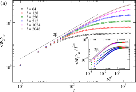
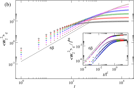
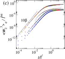
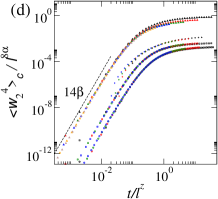
Figure 1: (Color online) (a) First and (b) second cumulants of SLRDs as a function of time $t$, calculated in different box sizes $l$ for $d=1+1$ surfaces of the Etching model. The insets of (a) and (b) and the plots in (c) and (d) show the collapse of the rescaled cumulants for all KPZ models in $d=1+1$. From bottom to top, collapsed curves for RSOS, SS, Eden and Etching models are shown. The dashed lines have the indicated slopes, where $\beta=1/3$.

III.1 SLRDs

The first cumulant (the mean) of the SLRDs, $\left\langle w_{2}\right\rangle_{c}$, is the squared local roughness - a standard quantity in the analysis of fluctuating interfaces Krug (1997). In KPZ systems, the scaling of $\left\langle w_{2}\right\rangle_{c}$ in time $t$ and box size $l$ is given by the Family-Vicsek (FV) Family and Vicsek (1985) scaling $\left\langle w_{2}\right\rangle_{c}\sim l^{2\alpha}f_{1}\left(t/l^{z}\right)$, where $f_{1}(x)$ is a scaling function behaving as $f_{1}(x)\approx const.$ for $x\gg 1$ and $f_{1}(x)\sim x^{2\beta}$ for $x\ll 1$, with $\beta=\alpha/z$ being the growth exponent. Therefore, for small times $(t\ll l^{z})$, so that the lateral correlation length ($\xi\sim t^{1/z}$) is smaller than $l$, $\left\langle w_{2}\right\rangle_{c}\sim t^{2\beta}$. On the other hand, for $t\gg l^{z}$ (i. e, for $\xi\gg l$), $\left\langle w_{2}\right\rangle_{c}$ becomes constant in time and scales as $\left\langle w_{2}\right\rangle_{c}\sim l^{2\alpha}$. This well-known scaling is shown in Fig. 1a for the ($1+1$) Etching model.

From the FV scaling, we might expect, for the $n$th cumulant of SLRDs, that

$$\left\langle w_{2}^{n}\right\rangle_{c}\sim l^{2n\alpha}f_{n}\left(t/l^{z}\right),$$ (5)

as is, indeed, confirmed in the insets of Figs. 1a-b and Figs. 1c-d by the nice collapse of the rescaled cumulants for a given model, in $d=1+1$. Moreover, this scaling also holds in $d=2+1$, as shown in Figs. 2a and 2b for the RSOS and Etching models, respectively. In Fig. 1b, we see that $f_{2}(x)\approx const.$ for $t\gg l^{z}$, as expected. However, $\left\langle w_{2}^{2}\right\rangle_{c}$ depends on both $t$ and $l$ at short times. In general, we have found $\left\langle w_{2}^{n}\right\rangle_{c}\sim l^{(1-n)d_{s}}t^{\gamma_{n}}$, with the exponent $\gamma_{n}$ depending on the exponents $\beta$ and $\alpha$ (or $z$). Thus, $f_{n}(x)\sim x^{\gamma_{n}}$, rather than the simple behavior $f_{n}(x)\sim x^{2n\beta}$, which we could naively expect.

Actually, this $l$-dependence and non-trivial temporal scaling is not limited to KPZ systems, but a general feature of the cumulants of SLRDs, and also of (global) WDs, when $\xi\ll l$ (or $L$). For instance, a similar result can be proved for the EW class in $d=1+1$, for the global WD calculated by Antal and Rácz Antal and Rácz (1996) as a function of time. In fact, from the generating function of the moments calculated in Antal and Rácz (1996) it is straightforward to demonstrate that, at short times ($\xi\ll L$), $\left\langle W_{2}^{n}\right\rangle_{c}\sim L^{(1-n)}t^{\gamma_{n}}$, with $\gamma_{n}=n-1/2$ (see appendix A). Although $W_{2}$ is the global roughness (for PBC), we remark that, when $\xi\ll l\leq L$, the BCs becomes irrelevant, since most columns inside a given box are uncorrelated, and, thus, the same behavior shall be found for WBC. We have confirmed this through simulations of the Family model in $d=1+1$, where $\left\langle w_{2}^{n}\right\rangle_{c}\sim l^{(1-n)}t^{n-1/2}$ is indeed found.

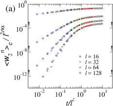
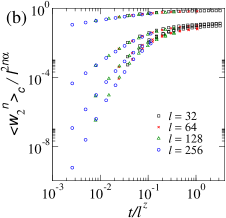
Figure 2: (Color online) First four rescaled SLRDs cumulants for the (a) RSOS and (b) Etching models in $d=2+1$. From top to bottom, curves for $n=1$, 2, 3 and 4 are shown. The exponents $\alpha=0.3869$ Pagnani and Parisi (2015) and $z=2-\alpha$ were used here.

Additional proof of the $l$-dependence in high order SLRDs’ cumulants is provided for the RD model, whose WD (calculated in appendix B) has $\left\langle W_{2}^{n}\right\rangle_{c}\sim L^{(1-n)d_{s}}t^{2n\beta}$. Since all heights are uncorrelated in this system, it is obvious that WD and SLRD are equivalent, so that $\left\langle w_{2}^{n}\right\rangle_{c}\sim l^{(1-n)d_{s}}t^{2n\beta}$. Noteworthy, the “expected” temporal scaling $\left\langle w_{2}^{n}\right\rangle_{c}\sim t^{2n\beta}$ is found in this case, suggesting that the correlation length (which is $\xi\sim 1$ here) is the responsible for the non-trivial $\gamma_{n}$ exponents in the other classes. In fact, for the $1+1$ EW class, where $\beta=1/4$ and $z=2$ Barabasi and Stanley (1995), one may write $\gamma_{n}=n-2\beta=2n\beta+(n-1)/z$ and, then, $\left\langle w_{2}^{n}\right\rangle_{c}\sim[l/\xi(t)]^{(1-n)}t^{2n\beta}$. The results for the ($1+1$) KPZ class (Fig. 1) are also consistent with this behavior. Therefore, the relevant measure in the finite-size scaling is $l_{R}=l/\xi(t)$, which gives the effective number of uncorrelated sites within a given box, so that, in general, $\left\langle w_{2}^{n}\right\rangle_{c}\sim l_{R}^{(1-n)d_{s}}t^{2n\beta}$.

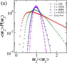
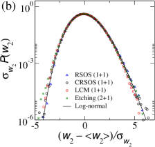
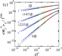
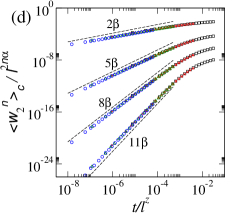
Figure 3: (Color online) Rescaled SLRDs for (a) $1+1$ SS model for $t=250$ and several $l$’s and (b) for several models with $t=100$ (25) and $l=2048$ (256) in $d=1+1$ ($2+1$). First four rescaled SLRDs cumulants for the (c) LCM and (d) CRSOS models in $d=1+1$. From top to bottom, curves for $n=1$, 2, 3 and 4 are shown. The dashed lines have the indicated slopes. In (a) $\alpha=3/2$, $\beta=3/8$ and $z=4$, and in (b) $\alpha=1$, $\beta=1/3$ and $z=3$ Barabasi and Stanley (1995).

The finite-size correction in the variance, $\left\langle w_{2}^{2}\right\rangle_{c}\sim 1/l_{R}^{d_{s}}$, can be simply understood noting that when $l_{R}^{d_{s}}$ random heights are summed, to obtain $\bar{h_{i}}$, $\bar{h_{i}^{2}}$ and, then, $w_{2,i}$, the central limit theorem states that the variance of the fluctuating variable $w_{2}$ will be of order $1/l_{R}^{d_{s}}$. So, when $l_{R}^{d_{s}}\rightarrow\infty$ (meaning that $t\rightarrow 0$ for a fixed $l$ or $l\rightarrow\infty$ for a fixed $t$) the SLRDs (and WDs) tends to a delta function, as pointed in Antal and Rácz (1996); Aarão Reis (2015). Interestingly, Antal and Rácz Antal and Rácz (1996) have showed that while the WD pdf of the $1+1$ EW class goes to a delta, it first approaches a log-normal distribution

$$P(x,t)=\frac{1}{\sqrt{2\pi}\sigma_{x}x}{\exp\left[{-\frac{(\ln(x)-\mu)^{2}}{2\sigma_{x}^{2}}}\right]},$$ (6)

with $x=w_{2}/\left\langle w_{2}\right\rangle$. We claim that, instead of a particularity of the $1+1$ EW class, this is a general feature of random (or almost random) interfaces. Indeed, in appendix B, we demonstrate that the SLRD/WD pdf for the RD approaches the log-normal (with $\mu=0$), when $l,L\gg 1$. Figure 3a shows scaled SLRDs for the $1+1$ SS (KPZ) model for a fixed $t$ and different $l$’s and, for large $l$’s (when $\xi\ll l$) they are well-fitted by Eq. 6. The limit $\xi\gg l$ will be discussed in Sec. IV. The same behavior is found in all universality classes in $d=1+1$ and $2+1$, for $\xi\ll l$, as shown in Fig. 3b. As shown in appendix B, if the variance of the log-normal scales as $\left\langle x^{2}\right\rangle_{c}\sim 1/l_{R}^{d_{s}}$, the high order cumulants shall be $\left\langle x^{n}\right\rangle_{c}\sim l_{R}^{(1-n)d_{s}}$, which explains the behavior $\left\langle w_{2}^{n}\right\rangle_{c}\sim l_{R}^{(1-n)d_{s}}t^{2n\beta}$. Finally, since $l_{R}\sim l/t^{1/z}$, in general, one has $\left\langle w_{2}^{n}\right\rangle_{c}\sim l^{(1-n)d_{s}}t^{\gamma_{n}}$ with

$$\gamma_{n}=2n\beta+\frac{(n-1)d_{s}}{z}=\left[2n+\frac{(n-1)d_{s}}{\alpha}\right]\beta.$$ (7)

In fact, for the RD model, where $\alpha,z\rightarrow\infty$ Barabasi and Stanley (1995), $\gamma_{n}=2n\beta$ is recovered. For KPZ class, $\alpha=1/2$, in $d=1+1$, yields $\gamma_{n}=(2n-1)2\beta$ as, indeed, observed in Fig. 1. Moreover, the scaled SLRDs cumulants for the LCM model (MH class) and the CRSOS model (VLDS class), shown, respectively, in Figs. 3c and 3d, have a nice scaling with $\gamma_{n}^{MH}=[2(4n-1)/3]\beta$ and $\gamma_{n}^{VLDS}=(3n-1)\beta$ for several decades in time. Since, $\alpha^{MH}=3/2$ and $\alpha^{VLDS}=1$, this confirms the general validity of the scaling law (7).

model		$\gamma_{1}$		$\gamma_{2}$		$\alpha$		$\beta$
RSOS		$0.483(9)$		$2.189(5)$		$0.39(1)$		$0.242(5)$
SS		$0.48(1)$		$2.20(1)$		$0.39(1)$		$0.240(5)$
Etching		$0.47(1)$		$2.18(2)$		$0.38(2)$		$0.235(5)$

Table 2: Exponents from $\left\langle w_{2}^{n}\right\rangle_{c}\sim t^{\gamma_{n}}$, with $n=1$ and $n=2$, and the corresponding scaling exponents $\beta=\gamma_{1}/2$ and $\alpha=\gamma_{1}/(\gamma_{2}-2\gamma_{1})$ for KPZ models in $d=2+1$.

Therefore, from estimates of the $\gamma_{n}$’s, it is possible to obtain the “classical” exponents $\alpha$, $\beta$ and $z$ from Eq. 7. For example, the values of $\gamma_{n}$ - calculated by estimating the effective exponents $\gamma_{n}^{eff}$ as the maxima of the successive slopes from the curves of $\ln\left\langle w_{2}^{n}\right\rangle_{c}\times\ln t$ and, then, extrapolating $\gamma_{n}^{eff}$ for large $l$’s - for KPZ models in $d=2+1$ are displayed in Tab. 2. The exponents $\alpha$ and $\beta$ obtained from them are in nice agreement with the best estimates known from the global roughness scaling ($\alpha=0.3869(4)$ and $\beta\approx 0.24$) Pagnani and Parisi (2015).

We remark that the usual way to determine $\alpha$ is to grow the interface until the steady state for different substrate sizes $L$ and then use the saturation roughness ($W_{sat}$) scale: $W_{sat}\sim L^{\alpha}$. However, usually, this requires long simulational times and, thus, the best available results are limited to relatively small $L$’s, mainly in $d\geqslant 2+1$ Kelling and Ódor (2011); Pagnani and Parisi (2015), where finite-size effects can play a relevant role. More important, it is very hard to attain the steady state in experiments and, thence, the possibility of estimating $\alpha$ from a temporal scaling, as devised here, is of paramount importance.

Actually, in systems following the FV scaling, $\alpha$ can be obtained in the growth regime from the scaling of the local roughness with the box size $l$ ($\left\langle w_{2}\right\rangle_{c}\sim l^{2\alpha_{loc}}$, where $\alpha_{loc}$ is the local roughness exponent), since $\alpha=\alpha_{loc}$. However, this scaling usually have strong corrections and may be also featured by crossover effects due to grain/mound structures at surface Oliveira and Aarão Reis (2007b); *tiago11Graos2. Even worse, several systems present anomalous scaling, so that $\alpha\neq\alpha_{loc}$ López (1999); *ramasco00. For instance, the scaling of the LCM model (the MH class), in $d=1+1$, is anomalous and $\alpha_{loc}=1$ whereas $\alpha=3/2$. As confirmed in Fig. 3c, the temporal scaling of the MH SLRDs’ cumulants yields the (global) exponent $\alpha$.

Reliable estimates of the correlation length $\xi(t)$ - and, consequently, of the dynamic exponent $z$ (from $\xi\sim t^{1/z}$) - are also difficult to obtain, for example, in surfaces with multipeaked grains/mounds Almeida et al. (2014, 2015). So, the possibility of calculating $z$ from a simple measure such as $\left\langle w_{2}^{n}\right\rangle_{c}$ is very useful. Indeed, from Eq. 7, one has $z=2/(\gamma_{2}-2\gamma_{1})$ and, then, using the values in Tab. 2, we find $z=1.63(3)$ (RSOS), $1.61(3)$ (SS) and $1.61(4)$ (Etching), again, in good agreement with the best known estimate ($z\approx 1.613$ Pagnani and Parisi (2015)).

III.2 LEHDs

At the PBC steady state, the mean (global) maximal relative height $\left\langle M_{sat}\right\rangle_{c}$ scales as the surface roughness $\left\langle M_{sat}\right\rangle_{c}\sim\left\langle W_{sat}\right\rangle\sim L^{\alpha}$ Raychaudhuri et al. (2001). The only known exception is the EW class in $d=2+1$, where $\left\langle W_{sat}\right\rangle\sim\sqrt{\ln{L}}$ and $\left\langle M_{sat}\right\rangle_{c}\sim\ln{L}$ Lee (2005); Oliveira and Aarão Reis (2008). Anyway, in most cases, this suggests for the cumulants of the local MAHDs that

$$\left\langle M^{n}\right\rangle_{c}\sim l^{n\alpha}g_{n}\left(t/l^{z}\right),$$ (8)

where the scaling function $g_{n}(x)$ would scale as $g_{n}(x)\sim const.$ for $x\gg 1$ and $g_{n}(x)\sim x^{\delta_{n}}$ for $x\ll 1$. This scaling is confirmed in Figs. 4a-4d by the good collapse of the high order ($n>1$) rescaled cumulants of the MAHDs for the KPZ models in $d=1+1$. However, for the mean $n=1$ (Fig. 4a) reasonable collapses are observed only for the larger $l$’s. Indeed, Raychaudhuri et al. Raychaudhuri et al. (2001) demonstrated that the (global) maximal relative height increases in time as $\left\langle M_{g}\right\rangle\sim t^{\beta}\left[C+\ln{L}-\left(\beta/\alpha\right)\ln{t}\right]^{1/a}$, where $C$ is a constant and the exponent $a$ is associated to the decay of the right tail either of the extremal height distribution or the velocity distribution. Therefore, the origin of the deviation in $\left\langle M\right\rangle_{c}$ (Fig. 4a) is certainly these logarithmic enhancements. It is impressive that such logarithmic seem not be present in the high order cumulants.

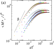
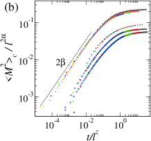
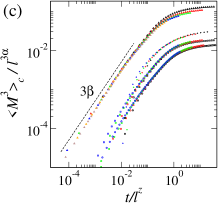
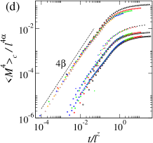
Figure 4: (Color online) (a) First, (b) second, (c) third and (d) forth rescaled cumulants of MAHDs, calculated in different box sizes $l$. From bottom to top, collapsed curves for RSOS, SS, Eden and Etching models in $d=1+1$ are shown. The dashed lines have the indicated slopes, where $\beta=1/3$.

As a consequence of the finite-time and -size effects, the scaling of $\left\langle M\right\rangle_{c}$ in time is not so clear, but is initially consistent with $\left\langle M\right\rangle_{c}\sim t^{\beta}$ (see Fig. 4a). On the other hand, for the higher order cumulants (Figs. 4b-4d), we find good power laws $\left\langle M^{n}\right\rangle_{c}\sim t^{n\beta}$. Thus, $g_{n}(x)\sim x^{n\beta}$ for $x\ll 1$, meaning that (asymptotically) $\left\langle M^{n}\right\rangle_{c}$ does not depend on $l$, for $t\ll l^{z}$, in contrast with $\left\langle w_{2}^{n}\right\rangle_{c}$. This happens because fluctuations in $M_{i}$ is dominated by $h_{max,i}$, which is not an average and, so, does not follow the central limit theorem. Therefore, it is not possible to determine $\alpha$ (and $z$) directly from $\left\langle M^{n}\right\rangle_{c}$ vs. $t$, but alternative measures of $\beta$ can be found.

For the RSOS, SS and Eden models, Fig. 4 shows that $\left\langle M^{n}\right\rangle_{c}$ deviate from the scaling at early times. This is due to the very smooth surfaces produced by these models at short times, which are almost flat inside a box ($M_{i}\lesssim 1$). In contrast, even for small $t$, the interfaces of the Etching model have a considerable roughness and, consequently, a well-behaved $\left\langle M^{n}\right\rangle_{c}$ scaling.

The cumulants of the local MIHDs, $\left\langle m^{n}\right\rangle_{c}$, follows a scale similar to Eq. 8, as shown in Fig. 5 for the RSOS model. However, the scaling functions $g_{n}^{min}(x)$ for $n=3$ and $4$ have a crossover at $t\ll l^{z}$, leading to deviations of the scaling $g_{n}^{min}(x)\sim x^{n\beta}$. Similar results were found for the other models in $d=1+1$.

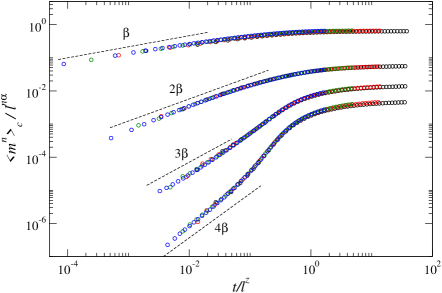
Figure 5: (Color online) First four rescaled cumulants of MIHDs for the RSOS model in $d=1+1$. From top to bottom, curves for $n=1$, 2, 3 and 4 are shown. The dashed lines have the indicated slopes, with $\beta=1/3$.

In two dimensions, the cumulants of MAHDs and MIHDs present stronger corrections than in $d=1+1$ and rescaling them according to Eq. 8 does not lead to good data collapse (not shown). So, in general, we may conclude that while the scaling of cumulants of the SLRDs is a powerful method to obtain the scaling exponents, the same does not happen with the one of the LEHDs.

IV Squared Local roughness distributions

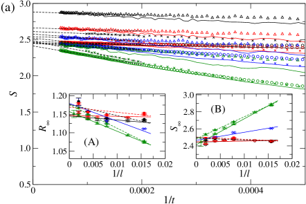
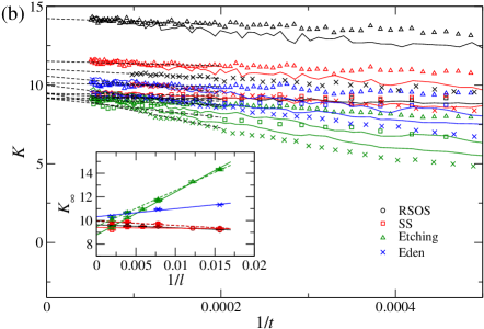
Figure 6: (Color online) (a) Skewness and (b) kurtosis as functions of $1/t$ for all KPZ models in $d=1+1$, calculated in boxes of sizes $l=64$ (black), $128$ (red), $256$ (blue) and $512$ (green). For RSOS, SS and Etching models, symbols are for growth on fixed size substrates, whilst full lines for enlarging ones. In (a), the insets show the extrapolated (in time) ratios (A) $R_{\infty}$ and (B) $S_{\infty}$. The extrapolated kurtosis are displayed in the inset of (b). In insets, open and full symbols are data for fixed size and enlarging substrates, respectively, while full and dashed lines are linear fits of them.

Figures 6a and 6b show the extrapolation of the skewness $S$ and kurtosis $K$ of the SLRDs, for $t\rightarrow\infty$ (i. e., for the regime of $\xi\gg l$), for the KPZ models in $d=1+1$ in both fixed size (symbols) and enlarging substrates (full lines). In all cases, good linear behaviors are found if we use $1/t$ in the abscissa, for long times. The extrapolated values $S_{\infty}$, $K_{\infty}$, and also of the ratio $R_{\infty}$, are displayed in the insets of Fig. 6. For RSOS and SS models, they present negligible $l$-dependences, allowing us to obtain accurate estimates of those ratios, whose averages are depicted in Tab. 3. On the other hand, stronger finite-size effects are observed in SLRDs of Eden and (mainly) of the Etching models. In the latter, this is certainly due to a large intrinsic width $w^{2}_{i}$ dominating the roughness at short scales. In fact, following the procedures and definitions in Ref. Alves et al. (2014b), we estimate here $\left\langle w^{2}_{i}\right\rangle=2.21(2)$ for the Etching model (in $d=1+1$). However, contrarily to its original version, for the Eden model, we do not find a correction consistent with an intrinsic width, so, it has other origin, possibly the existence of some remaining anisotropy at short scales. Anyway, for large $l$’s, we may observe those ratios converging towards the ones for SS/RSOS models. As noted by Halpin-Healy and Takeuchi Halpin-Healy and Takeuchi (2015), the SLRD by Antal et al. Antal et al. (2002) - calculated for steady state EW interfaces with WBC - should be also the pdf of $1+1$ SLRDs of KPZ class. Indeed, this pdf has ratios $R=1.12$, $S=2.55$ and $K=10.27$ that, although do not agree with our estimates within the error bars, are very close to them. A similar slight difference has been reported for the Euler integration of the KPZ equation Halpin-Healy and Takeuchi (2015).

In $d=2+1$, we find $R$, $S$ and $K$ extrapolating nicely, again, as $1/t$. The obtained $S_{\infty}$ and $K_{\infty}$ are displayed in Figs. 7a and 7b, respectively, where some finite-size effects are observed even for the RSOS and SS models, and more severe corrections in the Etching one (in this case we estimate $\left\langle w^{2}_{i}\right\rangle=2.7(1)$). Notwithstanding, again, as size increases these ratios converges to similar asymptotic places. The estimates for RSOS and SS models are depicted in Tab. 3, where we see that $S$ and $K$ as a nice agreement with the estimates from the Euler integration of KPZ equation Halpin-Healy and Palasantzas (2014) ($S=2.03$ and $K=7.11$). Moreover, the $R$ value is a bit larger than the estimate $1/R=0.53(2)$ in Aarão Reis (2015). For the Etching model, despite the stronger corrections, we find $R\approx 2.08$, $S\approx 1.95$ and $K\approx 6.4$. Whilst $R$ agrees with other models, the difference in $S$ and $K$ from the bottom limits are, respectively, $2.5$% and $8.5$%.

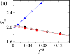
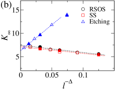
Figure 7: (Color online) Extrapolated ($t\rightarrow\infty$) (a) skewness and (b) kurtosis of SLRDs as functions of $1/l^{\Delta}$, for KPZ models grown on fixed size (open) and enlarging substrates (full symbols) in $d=2+1$. The dashed lines are linear fits of the data. $\Delta=1$ for RSOS and SS and $\Delta=1.25$ for Etching model.

dimension		$R$		$S$		$K$
$1+1$		$1.15(2)$		$2.44(4)$		$9.5(4)$
$2+1$		$2.05(5)$		$2.04(4)$		$7.3(3)$

Table 3: Cumulant ratios for KPZ SLRDs.

These results show that our extrapolation procedure (first in time, (A) to guarantee that $\xi\gg l$ and, then, for large $l$’s, (B) to overcome finite-size effects) is a reliable way to access the universality of local distributions. We recall that in recent works Almeida et al. (2014); Halpin-Healy and Palasantzas (2014); Halpin-Healy and Takeuchi (2015); Brandt et al. (2015); Aarão Reis (2015) this was achieved by performing simulations for very long growth times, to fulfill the requisite (A), and for several box sizes, in order (to try) to determine a plateau - a $l$-independent value of $R$, $S$ and $K$. Temporal extrapolations of the maxima (when they exist) of these plateaus can be also worthy Aarão Reis (2015). However, to observe clear (wide) plateaus in systems with strong finite-size corrections, huge growth times can be necessary. This was, indeed, observed for the ($2+1$) Etching model in Aarão Reis (2015). A similar problem shall happen in systems with large $z$, whose $\xi$’s increase very slowly in time. Moreover, in experiments, the limited number of samples and/or small $\xi$’s might prevent the observation of reliable plateaus.

On the other hand, within our framework, the temporal extrapolation provides good estimates of the cumulant ratios (for $\xi\gg l$) from data for (relatively) short deposition times. For comparison, Aarão Reis Aarão Reis (2015) has obtained $2.0\leq S\leq 2.2$ from simulations of the RSOS model, in $d=2+1$, for times up to $t=13000$, while we find here $S=2.04(4)$ from data for $t=1000$. Obviously, the temporal extrapolations cannot be done for arbitrarily short times, but we observe that working with $t$’s so that $\xi(t)\sim l$ is enough, which is much easier to work than $\xi\gg l$. For instance, recalling that $\xi=(\sqrt{A}|\lambda|t)^{1/z}$ Krug et al. (1992) and using the values of $A$ and $\lambda$ in Carrasco et al. (2014), for $t=1000$ (in $d=2+1$), one has $\xi_{SS}\approx 52$ and good extrapolations were possible for $l\lesssim 64$. In $d=1+1$, $\xi_{SS}\approx 737$ for $t=20000$ and we have worked with $l\leq 512$.

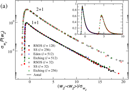
Figure 8: (Color online) Rescaled SLRDs for KPZ models in $d=1+1$ (bottom) and $d=2+1$ (top). Data for $d=2+1$ was shifted up two decades. Inset shows the same SLRDs in linear scaling, with data for $d=2+1$ centered in 5. Data for fixed size (RSOS and Etching) and enlarging substrates (SS) are shown.

Another interesting finding here is that the asymptotic KPZ SLRDs are the same for flat (fixed size) and curved (enlarging substrates) geometries. Indeed, in Fig. 6, we see that for long times $S$ (and also $K$), for the same model and $l$, tends to become equal regardless the substrate enlarges or not. This leads to temporal extrapolations $S_{\infty}$ and $K_{\infty}$ very similar for both subclasses. In $d=2+1$, this is even more evident (see the superimposed data in Fig. 7). Moreover, the asymptotic cumulant ratios for the (really curved) Eden surfaces agree quite well with the ones for other (flat surface) models, in $d=1+1$.

The rescaled SLRDs in $d=1+1$ and $d=2+1$ are shown in Fig. 8. The nice collapse of the distributions for different models, boxes sizes and geometries gives a final confirmation of their universality in both dimensions. We remark that SRLDs for Eden and Etching models for small $l$’s (not shown) do not present a good collapse, as expected from the corrections observed in their cumulant ratios. The Antal et al. Antal et al. (2002) pdf is also shown in Fig. 8 and presents an excellent agreement with the $1+1$ SLRDs. Thus, despite the small differences in their cumulant ratios, our results confirm the claim of Halpin-Healy and Takeuchi Halpin-Healy and Takeuchi (2015) that the steady state EW distribution also plays the role in KPZ growth regime, when WBC is considered. Concerning the right tail of the SLRDs, we find evidences of an exponential (in $d=1+1$) and stretched exponential (in $d=2+1$) decay, as also suggested in Halpin-Healy and Takeuchi (2015) and Paiva and Aarão Reis (2007); Halpin-Healy and Palasantzas (2014), respectively.

V Extremal relative height distributions

We start this section remarking that the MAHDs and MIHDs are directly related to the decay of the right and left tails, respectively, of the HDs. Since RSOS and SS models have HDs with $S<0$, their left (right) tails are equivalent to the right (left) ones of Eden and Etching models (whose HDs have $S>0$). Therefore, we will compare MIHDs of the former models with the MAHDs of the last ones, and vice-versa.

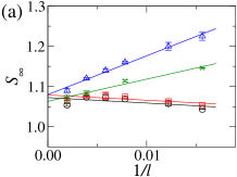
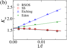
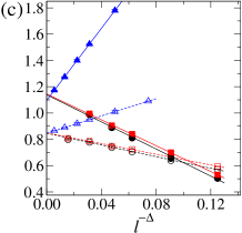
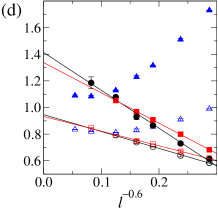
Figure 9: (Color online) Extrapolated (a) skewness and (b) kurtosis for LEHDs of KPZ models in $d=1+1$. For $d=2+1$, the extrapolated skewness (open) and kurtosis (full symbols) are shown in (c) for MAHDs and (d) for MIHDs. In (c), $\Delta=1$ for RSOS/SS and $\Delta=1.25$ for Etching model.

Performing an analysis of cumulant ratios of local MAHDs and MIHDs similar to the previous section, we find that they also extrapolate in time as $1/t$. The long time values obtained for $S$ and $K$ in $d=1+1$ are shown in Figs. 9a and 9b, respectively. Again, strong finite-size corrections are found for Eden and Etching models, but, after a size extrapolation, we find accurate estimates of $R$, $S$ and $K$ (depicted in Tab. 4). Since the stationary (within a box of size $l\ll\xi$) HDs are symmetric in $d=1+1$, MAHDs and MIHDs are identical. We recall that in Halpin-Healy and Takeuchi (2015) it was claimed that the Majumdar-Comtet (M-C) Majumdar and Comtet (2004) pdf - for (global) extremal heights of steady state $1+1$ EW interfaces with free BC - also represents the local MAHDs of $1+1$ KPZ systems. Indeed, our estimates for $S$ and $K$ are just slight smaller than the ones for the M-C distribution ($R=2.98$, $S=1.11$ and $K=1.69$), while $R$ agree within the error bar.

dimension		$R$		$S$		$K$
$1+1$		$3.00(5)$		$1.07(2)$		$1.60(3)$
$2+1$-MAHDs		$7.3(4)$		$0.84(2)$		$1.14(5)$
$2+1$-MIHDs		$7.3(4)$		$0.93(3)$		$1.35(10)$

Table 4: Cumulant ratios for KPZ LEHDs.

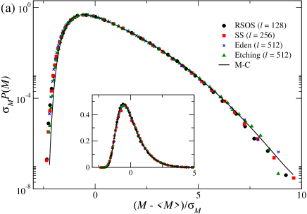
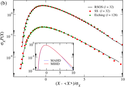
Figure 10: (Color online) (a) Rescaled LEHDs for KPZ models in $d=1+1$. Inset shows the same data in linear scale. (b) Rescaled MAHDs ($X=M$, top) and MIHDs ($X=m$, bottom) for KPZ models in $d=2+1$. MAHDs (MIHDs) were shifted two decades up (down). The non-shifted MAHD and MIHD of the RSOS model are displayed in the inset. Data for fixed size (RSOS and Etching) and enlarging substrates (SS) are shown.

For $d=2+1$, the stationary KPZ HD is asymmetric and, so, different LEHDs are expected. Indeed, different values for $S$ and $K$ are found for MA- and MIHDs for RSOS/SS models (see Tab. 4). The MAHDs’ ratios for the Etching model extrapolate to almost the same values, while the ones for MIHDs can not be extrapolated, due to a non-monotonic behavior (see Fig. 9d). It is worth to mention that in Ref. Halpin-Healy and Palasantzas (2014) $S=0.884/0.877$ and $K=1.20/1.17$ were reported for MA/MIHDs for the Euler integration of KPZ equation, which are quite close our estimates in most cases.

Figures 10a and 10b show the rescaled LEHDs for $d=1+1$ and $2+1$, respectively. In the one-dimensional case, an excellent data collapse for all models and a nice agreement with the M-C pdf in the peaks and right tails are observed, but a slight difference exits in the left tail, as also found in Halpin-Healy and Takeuchi (2015). In $d=2+1$, again, MAHDs (and MIHDs) for different models collapse quite well. As expected, from their similar cumulant ratios (Tab. 4), rescaled (2+1) KPZ MAHDs and MIHDs are very similar, presenting some difference only in their right tail (see inset of Fig. 10b).

VI Final discussions and Conclusion

In summary, we have presented a detailed numerical analysis of experimentally relevant local distributions of squared roughness (SLRDs) and extremal heights (LEHDs) - calculated in the growth regime of several models in one- and two-dimensions.

Strong finite-size effects were found in the distributions of some KPZ models, but strong evidences of their universality was obtained after appropriate extrapolations of their cumulant ratios. We claim that the procedure devised here advances over previous analysis of local distributions, since reliable estimates of cumulant ratios are obtained for relatively short times (so that $\xi\sim l$), instead of long times ($\xi\gg l$). This can be very important in the analysis of experimental interfaces, where typically $\xi$ is small and/or in universality classes with large $z$. We also emphasize that the cumulant ratio $R$, disregarded in most of previous works on local distributions, can be very useful to decide the universality class of a given system. For instance, local distributions for the MH class in $d=2+1$ have been recently studied in Brandt et al. (2015), where $R\approx 4$, $S\approx 0.88$ and $K\approx 0.85$ were found for the MAHDs ($=$ MIHDs in this class). Comparing these values with the ones in Tab. 4, we see that $S$ and $K$ are close to the KPZ ones, but a remarkable difference exists in $R$.

Although the underlying height fluctuations, temporal and spatial covariances, are different for flat and curved KPZ interfaces (in the growth regime) of KPZ interfaces, we find here that SRLDs and LEHDs do not present this dependence. Indeed, within a box of size $l\ll\xi$, we obtain stationary measures of $w_{2}$, $M$ and $m$ and, thus, our results are showing that stationary fluctuations in curved interfaces are the same as in flat ones.

Another very important finding here was the scaling of the SLRDs’ cumulants at early times. We stress that this scaling advances over other methods to calculate these exponents because it is not necessary to grow the interface until the steady-state (which, generally, demands long growth/simulation times) to obtain $\alpha$ and $z$. Moreover, this (temporal) scaling seems do not suffer from crossover effects and is not affected by scaling anomalies, as does the local roughness scaling with the box size $l$. Another advantage of this method is that smooth curves of $\left\langle w_{2}^{n}\right\rangle_{c}\times t^{\gamma_{n}}$ can be obtained even for a small number of surfaces (samples), since the cumulants are averaged over several boxes at surface. Thus, we believe that this method will be very useful in experimental studies. Furthermore, it can also be important to solve theoretical/numerical issues as, for example, the KPZ exponents in higher dimensions and its related upper critical dimension.

Appendix A Cumulants of the SLRD of EW class in $d=1+1$

Antal and Rácz Antal and Rácz (1996) have calculated the global roughness distribution $P(W_{2},t)$ of $1+1$ EW interfaces with PBC. For flat initial conditions, they found the generating function $G_{L}(\zeta,t)$ of its moments as

$$G_{L}(\zeta,t)=\mathcal{N}\prod_{m=1}^{\infty}\int dc_{m}dc_{m}^{*}\frac{\exp\left\{{-2|c_{m}|^{2}[\zeta+1/2\sigma_{m}^{2}(t)]}\right\}}{\sigma_{m}^{4}(t)},$$ (9)

where $\mathcal{N}$ is a normalization factor, $c_{m}$ (and $c_{-m}=c_{m}^{*}$) are the coefficients of the Fourier expansion of $h(x,t)-\bar{h}(t)$ and

$$\sigma_{m}^{2}(t)=\frac{D(1-e^{-2\nu q_{m}^{2}t})}{L\nu q_{m}^{2}},$$ (10)

with $q_{m}=2\pi m/L$. Defining $\left\langle W_{2}\right\rangle_{s}=DL/(12\nu)$ (the steady state squared roughness) and $\tau\equiv 8\pi^{2}\nu t/L^{2}=4\pi^{2}[\xi(t)/L]^{2}$, one may write $\sigma_{m}^{2}(t)={3\left\langle W_{2}\right\rangle_{s}(1-e^{-m^{2}\tau})}/{(\pi m)^{2}}$. Calculating the Gaussian integrals, $G_{L}(\zeta,t)$ can be obtained as well as $\Psi_{L}(\zeta,t)\equiv\ln G_{L}(\zeta,t)$, which is the generating function of the cumulants of $P(W_{2},t)$, given by

$$\left\langle W_{2}^{n}\right\rangle_{c} = (-1)^{n}\left(\frac{\partial\Psi_{L}}{\partial\zeta}\right)_{\zeta=0}$$

$$= \frac{(n-1)!6^{n}\left\langle W_{2}\right\rangle_{s}^{n}}{\pi^{2n}}\sum_{m=1}^{\infty}\frac{(1-e^{-\tau m^{2}})^{n}}{m^{2n}}.$$

For short times, so that $\tau\ll 1$ (and, thus, $\xi\ll L$), this sum can be approached by an integral yielding

$$\left\langle W_{2}^{n}\right\rangle_{c}\sim\left\langle W_{2}\right\rangle_{s}^{n}\tau^{n-1/2}\sim(D^{n}/\sqrt{\nu})L^{1-n}t^{n-1/2}.$$ (12)

Appendix B SLRD of random interfaces

Considering a random deposition on a hypercube substrate of dimension $d_{s}$ and lateral size $\mathcal{L}=La$, where $a$ is the lattice constant, $P(W_{2},t)$ can be calculated by particularizing the Antal and Rácz Antal and Rácz (1996) results, noting that

i) $\nu=0$ in a random growth, so that the variance $\sigma_{m}^{2}(t)$ (in Eq. 10) have to be changed to $\sigma^{2}(t)=2Dt/L^{d_{s}}$. Therefore, $\sigma^{2}$ no longer depends on the Fourier mode $m$ and, thus, all integrals in Eq. 9 are identical; and

ii) a cutoff have to be introduced in the product (in Eq. 9) of the $L^{d_{s}}$ modes.

After these considerations, we find the generating function

$$G_{L}(\zeta,t)=(1+2\zeta\sigma^{2})^{-(L^{d_{s}}/2)}$$ (13)

and, then, the cumulants

$$\left\langle W_{2}^{n}\right\rangle_{c}\sim L^{d_{s}}\sigma^{2n}\sim L^{(1-n)d_{s}}D^{n}t^{n}.$$ (14)

Defining the adimensional variable $x=W_{2}/\left\langle W_{2}\right\rangle=W_{2}/(2Dt)$, it is easy to calculate the inverse Laplace transform

$$P(W_{2},t)=\int_{-i\infty}^{i\infty}\frac{d\zeta}{2\pi i}G(\zeta)e^{\zeta W_{2}}=\frac{1}{\left\langle W_{2}\right\rangle}\Phi(x,t),$$ (15)

where

$$\Phi(x,t)=\frac{k^{k}}{(k-1)!}x^{k-1}e^{-kx},$$ (16)

with $k\equiv L^{d_{s}}/2$. Interestingly, this pdf does not depend explicitly on the time, but does on system size. Its cumulants are $\left\langle x^{n}\right\rangle_{c}=(n-1)!/k^{n-1}$. Then, when the system size diverges ($k\rightarrow\infty$), $\left\langle x^{n}\right\rangle_{c}\rightarrow 0$ for $n>1$, while $\left\langle x\right\rangle_{c}=1$, i. e., the distribution tends to a delta function. By the way, notwithstanding, it approaches a log-normal distribution. In fact, performing an expansion of $\Phi$ around its mean, defining $\epsilon=x-1$ and $\sigma_{x}^{2}\equiv\left\langle x^{2}\right\rangle_{c}=1/k$, we may write

$$\Phi(x,t)=\left(\frac{k^{k}e^{-k}}{(k-1)!}\right)\exp\left[-\frac{\epsilon-\ln(1+\epsilon)}{\sigma_{x}^{2}}\right]/x,$$ (17)

whose term into parenthesis converges to $1/(\sqrt{2\pi}\sigma_{x})$ for large $k$, while $[\epsilon-\ln(1+\epsilon)]\approx\ln^{2}(x)/2+\epsilon^{3}/6$ for $\epsilon\ll 1$. Then,

$$\Phi(x,t)\simeq\frac{1}{\sqrt{2\pi}\sigma_{x}x}{e^{-\frac{\ln^{2}(x)}{2\sigma_{x}^{2}}}}\left(1-\frac{\epsilon^{3}}{6\sigma_{x}^{2}}\right).$$ (18)

Defining the distance from the mean in terms of the standard deviation $\epsilon\equiv b\sigma_{x}$, we see that the correction $b^{3}/(6\sqrt{k})$ vanishes for large $k$. We remark that the cumulants of this log-normal have the form $\left\langle x\right\rangle_{c}=e^{\sigma_{x}^{2}/2}$, and $\left\langle x^{n}\right\rangle_{c}=\left\langle x\right\rangle_{c}^{n}(e^{\sigma_{x}^{2}}-1)^{n-1}g_{n}$, for $n>1$, with $g_{n}=const.+\mathcal{O}(e^{\sigma^{2}})$. Thence, if $\sigma_{x}\sim 1/L^{d_{s}}$ one finds $\left\langle x\right\rangle_{c}=1$ and $\left\langle x^{n}\right\rangle_{c}\sim L^{(1-n)d_{s}}$.

References

- Kardar et al. (1986) M. Kardar, G. Parisi, and Y.-C. Zhang, Phys. Rev. Lett. 56, 889 (1986).
- Barabasi and Stanley (1995) A.-L. Barabasi and H. E. Stanley, Fractal Concepts in Surface Growth (Cambridge University Press, Cambridge, England, 1995).
- Kriecherbauer and Krug (2010) T. Kriecherbauer and J. Krug, J. Phys. A 43, 403001 (2010).
- Corwin (2012) I. Corwin, Random Matrices Theory Appl. 1, 1130001 (2012).
- Dean et al. (2015) D. S. Dean, P. Le Doussal, S. N. Majumdar, and G. Schehr, Phys. Rev. Lett. 114, 110402 (2015).
- Halpin-Healy and Zhang (1995) T. Halpin-Healy and Y.-C. Zhang, Physics Reports 254, 215 (1995).
- Ferrari et al. (2004) P. L. Ferrari, M. Prähofer, and H. Spohn, Phys. Rev. E 69, 035102 (2004).
- Einstein and Pimpinelli (2014) T. L. Einstein and A. Pimpinelli, J. Stat. Phys. 155, 1178 (2014).
- Sasamoto and Spohn (2010) T. Sasamoto and H. Spohn, Phys. Rev. Lett. 104, 230602 (2010).
- Amir et al. (2011) G. Amir, I. Corwin, and J. Quastel, Commun. Pure Appl. Math. 64, 466 (2011).
- Calabrese and Le Doussal (2011) P. Calabrese and P. Le Doussal, Phys. Rev. Lett. 106, 250603 (2011).
- Imamura and Sasamoto (2012) T. Imamura and T. Sasamoto, Phys. Rev. Lett. 108, 190603 (2012).
- Takeuchi and Sano (2010) K. A. Takeuchi and M. Sano, Phys. Rev. Lett. 104, 230601 (2010).
- Takeuchi et al. (2011) K. A. Takeuchi, M. Sano, T. Sasamoto, and H. Spohn, Sci. Rep. 1, 34 (2011).
- Yunker et al. (2013) P. J. Yunker, M. A. Lohr, T. Still, A. Borodin, D. J. Durian, and A. G. Yodh, Phys. Rev. Lett. 110, 035501 (2013).
- Tracy and Widom (1994) C. Tracy and H. Widom, Commun. Math. Phys. 159, 151 (1994).
- Baik and Rains (2000) J. Baik and E. M. Rains, J. Stat. Phys. 100, 523 (2000).
- Prähofer and Spohn (2002) M. Prähofer and H. Spohn, J. Stat. Phys. 108, 1071 (2002).
- Sasamoto (2005) T. Sasamoto, J. Phys. A 38, L549 (2005).
- Borodin et al. (2008) A. Borodin, P. L. Ferrari, and T. Sasamoto, Commun. Pure Appl. Math. 61, 1603 (2008).
- Alves et al. (2011) S. G. Alves, T. J. Oliveira, and S. C. Ferreira, Europhys. Lett. 96, 48003 (2011).
- Oliveira et al. (2012) T. J. Oliveira, S. C. Ferreira, and S. G. Alves, Phys. Rev. E 85, 010601 (2012).
- Alves et al. (2013) S. G. Alves, T. J. Oliveira, and S. C. Ferreira, J. Stat. Mech. 2013, P05007 (2013).
- Halpin-Healy and Lin (2014) T. Halpin-Healy and Y. Lin, Phys. Rev. E 89, 010103 (2014).
- Halpin-Healy (2012) T. Halpin-Healy, Phys. Rev. Lett. 109, 170602 (2012).
- Oliveira et al. (2013) T. J. Oliveira, S. G. Alves, and S. C. Ferreira, Phys. Rev. E 87, 040102(R) (2013).
- Halpin-Healy (2013) T. Halpin-Healy, Phys. Rev. E 88, 042118 (2013).
- Carrasco et al. (2014) I. S. S. Carrasco, K. A. Takeuchi, S. C. Ferreira, and T. J. Oliveira, New J. Phys. 14, 123057 (2014).
- Almeida et al. (2014) R. A. L. Almeida, S. O. Ferreira, T. J. Oliveira, and F. D. A. Aarão Reis, Phys. Rev. B 89, 045309 (2014).
- Halpin-Healy and Palasantzas (2014) T. Halpin-Healy and G. Palasantzas, Europhys. Lett. 105, 50001 (2014).
- Almeida et al. (2015) R. A. L. Almeida, S. O. Ferreira, I. R. B. Ribeiro, and T. J. Oliveira, Europhys. Lett. 109, 46003 (2015).
- Alves et al. (2014a) S. G. Alves, T. J. Oliveira, and S. C. Ferreira, Phys. Rev. E 90, 020103(R) (2014a).
- Foltin et al. (1994) G. Foltin, K. Oerding, Z. Rácz, R. L. Workman, and R. K. P. Zia, Phys. Rev. E 50, R639 (1994).
- Plischke et al. (1994) M. Plischke, Z. Rácz, and R. K. P. Zia, Phys. Rev. E 50, 3589 (1994).
- Rácz and Plischke (1994) Z. Rácz and M. Plischke, Phys. Rev. E 50, 3530 (1994).
- ao Reis (2005) F. D. A. A. ao Reis, Phys. Rev. E 72, 032601 (2005).
- Miranda and Aarão Reis (2008) V. G. Miranda and F. D. A. Aarão Reis, Phys. Rev. E 77, 031134 (2008).
- Kelling and Ódor (2011) J. Kelling and G. Ódor, Phys. Rev. E 84, 061150 (2011).
- Marinari et al. (2002) E. Marinari, A. Pagnani, G. Parisi, and Z. Rácz, Phys. Rev. E 65, 026136 (2002).
- Oliveira and Aarão Reis (2007a) T. J. Oliveira and F. D. A. Aarão Reis, Phys. Rev. E 76, 061601 (2007a).
- Antal and Rácz (1996) T. Antal and Z. Rácz, Phys. Rev. E 54, 2256 (1996).
- Antal et al. (2002) T. Antal, M. Droz, G. Györgyi, and Z. Rácz, Phys. Rev. E 65, 046140 (2002).
- Paiva and Aarão Reis (2007) T. Paiva and F. D. A. Aarão Reis, Surf. Sci. 601, 419 (2007).
- Halpin-Healy and Takeuchi (2015) T. Halpin-Healy and K. A. Takeuchi, J. Stat. Phys. 160, 794 (2015).
- Raychaudhuri et al. (2001) S. Raychaudhuri, M. Cranston, C. Przybyla, and Y. Shapir, Phys. Rev. Lett. 87, 136101 (2001).
- Györgyi et al. (2007) G. Györgyi, N. R. Moloney, K. Ozogány, and Z. Rácz, Phys. Rev. E 75, 021123 (2007).
- Majumdar and Comtet (2004) S. N. Majumdar and A. Comtet, Phys. Rev. Lett. 92, 225501 (2004).
- Schehr and Majumdar (2006) G. Schehr and S. N. Majumdar, Phys. Rev. E 73, 056103 (2006).
- Lee (2005) D.-S. Lee, Phys. Rev. Lett. 95, 150601 (2005).
- Oliveira and Aarão Reis (2008) T. J. Oliveira and F. D. A. Aarão Reis, Phys. Rev. E 77, 041605 (2008).
- Rambeau and Schehr (2010) J. Rambeau and G. Schehr, Europhys. Lett. 91, 60006 (2010).
- Brandt et al. (2015) I. S. Brandt, V. C. Zoldan, V. Stenger, C. C. Plá Cid, A. A. Pasa, T. J. Oliveira, and F. D. A. Aarão Reis, J. Appl. Phys. 118, 145303 (2015).
- Mullins (1957) W. W. Mullins, J. Appl. Phys. 28, 333 (1957).
- Herring (1951) C. Herring, in The Physics of Powder Metallurgy, edited by W. E. Kingston (McGraw-Hill, New York, USA, 1951).
- Aarão Reis (2015) F. D. A. Aarão Reis, J. Stat. Mech. 2015, P11020 (2015).
- Kim and Kosterlitz (1989) J. M. Kim and J. M. Kosterlitz, Phys. Rev. Lett. 62, 2289 (1989).
- Mello et al. (2001) B. A. Mello, A. S. Chaves, and F. A. Oliveira, Phys. Rev. E 63, 041113 (2001).
- Family (1986) F. Family, J. Phys. A 19, L441 (1986).
- Villain (1991) J. Villain, J. Phys. I 1, 19 (1991).
- Lai and Das Sarma (1991) Z.-W. Lai and S. Das Sarma, Phys. Rev. Lett. 66, 2348 (1991).
- Note (1) In the SS model, a pair of neighboring columns has to be duplicated in order to conserve the symmetry of up and down steps at surface.
- Eden (1961) M. Eden, in Proceedings of Fourth Berkeley Symposium on Mathematics, Statistics, and Probability, Vol. 4, edited by J. Neyman (University of California Press, Berkeley,California, 1961) pp. 223–239.
- Paiva and Ferreira (2007) L. R. Paiva and S. C. Ferreira, J. Phys. A 40, F43 (2007).
- Krug (1997) J. Krug, Adv. Phys. 46, 139 (1997).
- Family and Vicsek (1985) F. Family and T. Vicsek, J. Phys. A 18, L75 (1985).
- Pagnani and Parisi (2015) A. Pagnani and G. Parisi, Phys. Rev. E 92, 010101(R) (2015).
- Oliveira and Aarão Reis (2007b) T. J. Oliveira and F. D. A. Aarão Reis, J. Appl. Phys. 101, 063507 (2007b).
- Oliveira and Aarão Reis (2011) T. J. Oliveira and F. D. A. Aarão Reis, Phys. Rev. E 83, 041608 (2011).
- López (1999) J. M. López, Phys. Rev. Lett. 83, 4594 (1999).
- Ramasco et al. (2000) J. J. Ramasco, J. M. López, and M. A. Rodríguez, Phys. Rev. Lett. 84, 2199 (2000).
- Alves et al. (2014b) S. G. Alves, T. J. Oliveira, and S. C. Ferreira, Phys. Rev. E 90, 052405 (2014b).
- Krug et al. (1992) J. Krug, P. Meakin, and T. Halpin-Healy, Phys. Rev. A 45, 638 (1992).