A Multilevel Correction Method for Interior Transmission Eigenvalue Problem

Abstract

In this paper, we give a numerical analysis for the transmission eigenvalue problem by the finite element method. A type of multilevel correction method is proposed to solve the transmission eigenvalue problem. The multilevel correction method can transform the transmission eigenvalue solving in the finest finite element space to a sequence of linear problems and some transmission eigenvalue solving in a very low dimensional spaces. Since the main computational work is to solve the sequence of linear problems, the multilevel correction method improves the overfull efficiency of the transmission eigenvalue solving. Some numerical examples are provided to validate the theoretical results and the efficiency of the proposed numerical scheme.

1 Introduction

Recently, many researchers are interested in the transmission eigenvalue problem [3, 8, 9, 10, 11, 14, 15, 16, 20, 23]. The transmission eigenvalue problem arises in the study of the inverse scattering for inhomogeneous media which not only has theoretical importance [11, 14], but also can be used to estimate the properties of the scattering material [8, 10, 25] since they can be determined from the scattering data. In the past few years, significant progress of the existence of transmission eigenvalues and applications has been made. We refer the readers to the recent papers [3, 5, 11].

Meanwhile, there are also many papers to give the numerical treatment for the transmission eigenvalue problem and the associated interior transmission problem [1, 4, 5, 15, 17, 18, 19, 26, 27]. But there are few papers providing the corresponding theoretical analysis for their numerical methods due to the difficulty that the problem is neither elliptic nor self-adjoint. The paper [19] presents an accurate error estimate of the eigenvalue and eigenfunction approximations for the Helmhotz transmission eigenvalue problem based on the iterative methods (bisection and secant) from [26]. The first aim of this paper is to give a theoretical analysis of the finite element method for the transmission eigenvalue problem with the inhomogeneous media.

In the past few years, a new type of multilevel correction method is proposed to solve the eigenvalue problem [21, 22, 28]. In the multilevel correction scheme, the solution on the finest mesh can be reduced to a series of solutions of the eigenvalue problem in a very low dimensional space and a series of solutions of the boundary value problem on the multilevel meshes. This multilevel correction method gives a way to construct a type of multigrid scheme for the eigenvalue problem [19, 29, 30]. The second aim of this paper is to propose a multilevel correction method for the transmission eigenvalue problem based on the obtained error estimate results.

The rest of this paper is organized as follows. In Section 2, we introduce the transmission eigenvalue problem and the corresponding theoretical results about the eigenvalue distribution. The finite element method and the corresponding error estimates are given in Section 3. Section 4 is devoted to introducing a type of multilevel correction method for the transmission eigenvalue problem. In Section 5, four examples are presented to validate the theoretical results and the efficiency of the proposed numerical methods. Some concluding remarks are given in the last section.

2 Transmission eigenvalue problem

First, we introduce some notation and the transmission eigenvalue problem. The letter $C$ (with or without subscripts) denotes a generic positive constant which may be different at its different occurrences through the paper. For convenience, the symbols $\lesssim$, $\gtrsim$ and $\approx$ will be used in this paper. Notations $x_{1}\lesssim y_{1},x_{2}\gtrsim y_{2}$ and $x_{3}\approx y_{3}$, mean that $x_{1}\leq C_{1}y_{1}$, $x_{2}\geq c_{2}y_{2}$ and $c_{3}x_{3}\leq y_{3}\leq C_{3}x_{3}$ for some constants $C_{1},c_{2},c_{3}$ and $C_{3}$ that are independent of mesh sizes.

In this paper, we are concerned with the transmission eigenvalues corresponding to the scattering of acoustic waves by a bounded simply connected inhomogeneous medium $\Omega\subset\mathcal{R}^{d}$ ($d=2,3$). The transmission eigenvalue problem is to find $k\in\mathcal{C}$, $(w,v)\in H^{1}(\Omega)\times H^{1}(\Omega)$ such that

$$\left\{\begin{array}[]{rcll}-{\rm div}\big{(}A\nabla w\big{)}&=&k^{2}n(x)w,&{\rm in}\ \Omega,\\ -\Delta v&=&k^{2}v,&{\rm in}\ \Omega,\\ w-v&=&0,&{\rm on}\ \partial\Omega,\\ \frac{\partial w}{\partial\nu_{A}}-\frac{\partial v}{\partial\nu}&=&0,&{\rm on}\ \partial\Omega,\end{array}\right.$$ (2.1)

where $\nu$ is the unit outward normal to the boundary $\partial\Omega$. There exists a real number $\gamma>1$ such that the symmetric matrix $A(x)$ and the index of refraction $n(x)$ satisfy that

$$\xi\cdot A\xi>\gamma|\xi|^{2}\ \ \ \forall\xi\in\mathcal{R}^{d},\quad n(x)>\gamma,\ \ a.e.\ \ \mbox{in}\ \Omega.$$ (2.2)

Values of $k$ such that there exists a nontrivial solution $(w,v)$ to (2.1) are called transmission eigenvalues.

Remark 2.1.

As in [4, 13], the numerical method and analysis can be extended to the case that there exists a real number $0<\gamma<1$ such that the symmetric matrix $A(x)$ and the index of refraction $n(x)$ satisfy that

$$0<\xi\cdot A\xi<\gamma|\xi|^{2}\ \ \ \forall\xi\in\mathcal{R}^{d},\quad 0<n(x)<\gamma,\ \ a.e.\ \ \mbox{in}\ \Omega.$$ (2.3)

Obviously, the eigenvalue problem (2.1) can be transformed into the following version: Find $\lambda\in\mathcal{C}$, $(u,w)\in H^{1}(\Omega)\times H^{1}(\Omega)$ such that

$$\left\{\begin{array}[]{rcll}-{\rm div}\big{(}A\nabla w\big{)}+n(x)w&=&\lambda n(x)w,&{\rm in}\ \Omega,\\ -\Delta v+v&=&\lambda v,&{\rm in}\ \Omega,\\ w-v&=&0,&{\rm on}\ \partial\Omega,\\ \frac{\partial w}{\partial\nu_{A}}-\frac{\partial v}{\partial\nu}&=&0,&{\rm on}\ \partial\Omega,\end{array}\right.$$ (2.4)

where $\lambda=k^{2}+1$. In the following of this paper, we mainly consider this eigenvalue problem. There are some papers [3, 10, 11, 20, 23] being concerned with the distribution of the eigenvalues for the eigenvalue problem (2.4).

In this paper, in order to give the analysis, we define the function spaces $\mathbb{V}$ and $\mathbb{W}$ as follows

$$\mathbb{V} := \Big{\{}\mathbf{\Psi}:=(\varphi,\psi)\in H^{1}(\Omega)\times H^{1}(\Omega)\ |\ \varphi-\psi\in H_{0}^{1}(\Omega)\Big{\}},$$ (2.5)

$$\mathbb{W} := L^{2}(\Omega)\times L^{2}(\Omega)$$ (2.6)

equipped with the norms

$$\|\mathbf{\Psi}\|_{\mathbb{V}}=\Big{(}\|\varphi\|_{1}^{2}+\|\psi\|_{1}^{2}\Big{)}^{1/2}\ \ {\rm and}\ \ \|\mathbf{\Psi}\|_{\mathbb{W}}=\Big{(}\|\varphi\|_{0}^{2}+\|\psi\|_{0}^{2}\Big{)}^{1/2},$$

respectively, where $\mathbf{\Psi}=(\varphi,\psi)\in\mathbb{V}$.

For the simplicity of notation, we define two sesquilinear forms

$$a(\mathbf{U},\mathbf{\Psi}) = \big{(}A\nabla w,\nabla\varphi\big{)}+\big{(}n(x)w,\varphi\big{)}-\big{(}\nabla v,\nabla\psi\big{)}-\big{(}v,\psi\big{)},$$ (2.7)

$$b(\mathbf{U},\mathbf{\Psi}) = \big{(}n(x)w,\varphi\big{)}-\big{(}v,\psi\big{)},$$ (2.8)

where $\mathbf{U}=(w,v),\mathbf{\Psi}=(\varphi,\psi)\in\mathbb{V}$. The associated variational form for (2.4) can be defined as follows: Find $(\lambda,\mathbf{U})\in\mathcal{C}\times\mathbb{V}$ such that $\|\mathbf{U}\|_{\mathbb{W}}=1$ and

$$a(\mathbf{U},\mathbf{\Psi}) = \lambda b(\mathbf{U},\mathbf{\Psi}),\ \ \ \forall\mathbf{\Psi}\in\mathbb{V}.$$ (2.9)

Then the corresponding adjoint eigenvalue problem is: Find $(\lambda,\mathbf{U}^{*})\in\mathcal{C}\times\mathbb{V}$ such that $\|\mathbf{U}^{*}\|_{\mathbb{W}}=1$ and

$$a(\mathbf{\Psi},\mathbf{U}^{*}) = \lambda b(\mathbf{\Psi},\mathbf{U}^{*}),\ \ \ \forall\mathbf{\Psi}\in\mathbb{V}.$$ (2.10)

In order to analyze the properties of the eigenvalue problem (2.9), we introduce the so-called $\mathbb{T}$-coercivity (inf-sup condition) for the bilinear form $a(\cdot,\cdot)$ (see, e.g., [3, 4, 5, 6, 13]). In this paper, the notation $\mathbb{T}$ denotes an isomorphic operator from $\mathbb{V}$ to $\mathbb{V}$ which is defined as follows

$$\mathbb{T}\mathbf{\Psi} = (\varphi,2\varphi-\psi),\ \ \ \ \forall\mathbf{\Psi}\in\mathbb{V}.$$ (2.11)

Similarly to [3, 4, 5], in order to give the eigenvalue distribution of (2.4), we also state the following $\mathbb{T}$-coercivity properties (inf-sup conditions).

Theorem 2.1.

The bilinear forms $a(\cdot,\cdot)$ and $b(\cdot,\cdot)$ have the following inf-sup conditions ($\mathbb{T}$-coercivities):

$$\inf_{0\neq\mathbf{\Phi}\in\mathbb{V}}\sup_{0\neq\mathbf{\Psi}\in\mathbb{V}}\frac{a(\mathbf{\Phi},\mathbf{\Psi})}{\|\mathbf{\Phi}\|_{\mathbb{V}}\|\mathbf{\Psi}\|_{\mathbb{V}}}\geq\mu_{a},$$ (2.12)

$$\inf_{0\neq\mathbf{\Phi}\in\mathbb{V}}\sup_{0\neq\mathbf{\Psi}\in\mathbb{V}}\frac{a(\mathbf{\Psi},\mathbf{\Phi})}{\|\mathbf{\Psi}\|_{\mathbb{V}}\|\mathbf{\Phi}\|_{\mathbb{V}}}\geq\mu_{a},$$ (2.13)

and

$$\inf_{0\neq\mathbf{\Phi}\in\mathbb{W}}\sup_{0\neq\mathbf{\Psi}\in\mathbb{W}}\frac{b(\mathbf{\Phi},\mathbf{\Psi})}{\|\mathbf{\Phi}\|_{\mathbb{W}}\|\mathbf{\Psi}\|_{\mathbb{W}}}\geq\mu_{b},$$ (2.14)

$$\inf_{0\neq\mathbf{\Phi}\in\mathbb{W}}\sup_{0\neq\mathbf{\Psi}\in\mathbb{W}}\frac{b(\mathbf{\Psi},\mathbf{\Phi})}{\|\mathbf{\Psi}\|_{\mathbb{W}}\|\mathbf{\Phi}\|_{\mathbb{W}}}\geq\mu_{b},$$ (2.15)

for some positive constants $\mu_{a}$ and $\mu_{b}$.

Proof.

From the conditions of the matrix $A$ and the refraction index $n(x)$, the following estimates hold

$$a(\mathbf{\Psi},\mathbb{T}\mathbf{\Psi}) = (A\nabla\varphi,\nabla\varphi)+(n(x)\varphi,\varphi)-(\nabla\psi,\nabla(2\varphi-\psi))$$ (2.16)

$$\ \ \ \ -(\psi,(2\varphi-\psi))$$

$$\geq \gamma\|\varphi\|_{1}^{2}+\|\psi\|_{1}^{2}-2(\nabla\psi,\nabla\varphi)-2(\psi,\varphi)$$

$$\geq \Big{(}\gamma-\frac{1}{\delta}\Big{)}\|\varphi\|_{1}^{2}+\Big{(}1-\delta\Big{)}\|\psi\|_{1}^{2}$$

$$\geq C\|\mathbf{\Psi}\|_{\mathbb{V}}^{2}.$$

Since $\gamma>1$, we can choose $\delta\in\Big{(}\frac{1}{\gamma},1\Big{)}$ such that $a(\cdot,\cdot)$ is $\mathbb{T}$-coercive which means there exists a positive constant $\mu_{a}$ such that the desired result (2.12) holds. In the same way, we can also prove the result (2.13).

Similarly, it is easy to prove that

$$\ b(\mathbf{\Psi},\mathbb{T}\mathbf{\Psi}) = (n(x)\varphi,\varphi)-(\psi,2\varphi-\psi)$$ (2.17)

$$\geq \Big{(}\gamma-\frac{1}{\delta}\Big{)}\|\varphi\|_{0}^{2}+(1-\delta)\|\psi\|_{0}^{2}.$$

Since $\gamma>1$, we can choose $\delta\in\Big{(}\frac{1}{\gamma},1\Big{)}$ such that $b(\cdot,\cdot)$ is $\mathbb{T}$-coercive in $\mathbb{W}\times\mathbb{W}$ which means the inf-sup conditions (2.14) and (2.15) hold for some positive constant $\mu_{b}$. ∎

We introduce the operators $\mathbb{K},\ \mathbb{K}_{*}\in\mathcal{L}(\mathbb{V})$ defined by the equations

$$a(\mathbb{K}\mathbf{\Phi},\mathbf{\Psi})=b(\mathbf{\Phi},\mathbf{\Psi}),\ \ a(\mathbf{\Psi},\mathbb{K}_{*}\mathbf{\Phi})=b(\mathbf{\Psi},\mathbf{\Phi}),\ \ \ \ \ \forall\mathbf{\Phi},\mathbf{\Psi}\in\mathbb{V}.$$ (2.18)

From Theorem 2.1, it is easy to know the operator $\mathbb{K}$ and $\mathbb{K}_{*}$ are linear bijective operators. Then the eigenvalue problem (2.9) can be written as an operator form for $\lambda\neq 0$ (denoting $\mu:=\lambda^{-1}$):

$$\mathbb{K}\mathbf{U}=\mu\mathbf{U},$$ (2.19)

with

$$\mathbb{K}_{*}\mathbf{U}^{*}=\bar{\mu}\mathbf{U}^{*}$$ (2.20)

for the adjoint eigenvalue problem (2.10). The $\mathbb{T}$-coercivity conditions (2.12)-(2.13) and (2.14)-(2.15) guarantee that every eigenvalue $\lambda$ is nonzero. From (2.12) and (2.13) and the compact embedding theorem of Sobolev spaces, it is well known that the operators $\mathbb{K}$ and $\mathbb{K}_{*}$ are compact. Thus the spectral theory for compact operators gives us a complete characterization of the eigenvalue problem (2.9).

There is a countable set of eigenvalues of (2.9). Let $\lambda$ be an eigenvalue of problem (2.9). There exists a smallest integer $\alpha$ such that

$${\rm Null}((\mathbb{K}-\mu)^{\alpha})={\rm Null}((\mathbb{K}-\mu)^{\alpha+1}),$$ (2.21)

where ${\rm Null}$ denotes the null space and we use the notation $\mu=\lambda^{-1}$. Let

$$M(\lambda)=M_{\lambda,\mu}={\rm Null}((\mathbb{K}-\mu)^{\alpha}),\quad Q(\lambda)=Q_{\lambda,\mu}={\rm Null}(\mathbb{K}-\mu)$$

denote the algebraic and geometric eigenspaces, respectively. The subspaces $M(\lambda)$ and $Q(\lambda)\subset M(\lambda)$ are finite dimensional. The numbers $m={\rm dim}M(\lambda)$ and $q={\rm dim}Q(\lambda)$ are called the algebraic and the geometric multiplicities of $\mu$ (and $\lambda$). The vectors in $M(\lambda)$ are generalized eigenvectors. The order of a generalized eigenvector is the smallest integer $p$ such that $(\mathbb{K}-\mu)^{p}\mathbf{U}=0$ (vectors in $Q(\lambda)$ being generalized eigenvectors of order $1$). Let us point out that a generalized eigenvector $\mathbf{U}^{p}$ of order $p$ satisfies

$$a(\mathbf{U}^{p},\mathbf{\Psi}) = \lambda b(\mathbf{U}^{p},\mathbf{\Psi})+\lambda a(\mathbf{U}^{p-1},\mathbf{\Psi}),\ \ \ \ \forall\mathbf{\Psi}\in\mathbb{V},$$ (2.22)

where $\mathbf{U}^{p-1}$ is a generalized eigenvector of order $p-1$.

Similarly we define the spaces of (generalized) eigenvectors for the adjoint problem

$$M^{*}(\lambda)=M_{\lambda,\mu}^{*}={\rm Null}((\mathbb{K}_{*}-\bar{\mu})^{\alpha}),\quad Q^{*}(\lambda)=Q^{*}_{\lambda,\mu}={\rm Null}(\mathbb{K}_{*}-\bar{\mu}).$$

Note that $\mu$ is an eigenvalue of $\mathbb{K}$ ($\lambda$ is an eigenvalue of problem (2.9)) if and only if $\bar{\mu}$ is an eigenvalue of $\mathbb{K}_{*}$ (${\bar{\lambda}}$ is an eigenvalue of adjoint problem (2.10)) with the ascent $\alpha$ and the algebraic multiplicity $m$ for both eigenvalues being the same.

3 Finite element method for Transmission eigenvalue problem

Now, let us define the finite element approximations for the problem (2.9). First we generate a shape-regular decomposition of the computational domain $\Omega\subset\mathcal{R}^{d}\ (d=2,3)$ into triangles or rectangles for $d=2$ (tetrahedrons or hexahedrons for $d=3$). The diameter of a cell $K\in\mathcal{T}_{h}$ is denoted by $h_{K}$. The mesh diameter $h$ describes the maximum diameter of all cells $K\in\mathcal{T}_{h}$. Based on the mesh $\mathcal{T}_{h}$, we construct a finite element space denoted by $\mathbb{V}_{h}\subset\mathbb{V}$. The same argument as in the beginning of this section illustrates that the following discrete inf-sup conditions also hold

$$\|\mathbf{\Phi}_{h}\|_{\mathbb{V}}\lesssim\sup_{\mathbf{\Psi}_{h}\in\mathbb{V}_{h}}\frac{a(\mathbf{\Phi}_{h},\mathbf{\Psi}_{h})}{\|\mathbf{\Psi}_{h}\|_{\mathbb{V}}}\ \ {\rm and}\ \ \|\mathbf{\Phi}_{h}\|_{\mathbb{V}}\lesssim\sup_{\mathbf{\Psi}_{h}\in\mathbb{V}_{h}}\frac{a(\mathbf{\Psi}_{h},\mathbf{\Phi}_{h})}{\|\mathbf{\Psi}_{h}\|_{\mathbb{V}}}.$$ (3.1)

The standard finite element method for the problem (2.9) is defined as follows: Find $(\lambda_{h},\mathbf{U}_{h})\in\mathcal{C}\times\mathbb{V}_{h}$ such that $\|\mathbf{U}_{h}\|_{\mathbb{W}}=1$ and

$$a(\mathbf{U}_{h},\mathbf{\Psi}_{h}) = \lambda_{h}b(\mathbf{U}_{h},\mathbf{\Psi}_{h}),\ \ \ \ \ \forall\mathbf{\Psi}_{h}\in\mathbb{V}_{h}.$$ (3.2)

Similarly, the discretization for the adjoint problem (2.10) can be defined as: Find $(\lambda_{h},\mathbf{U}_{h}^{*})\in\mathcal{C}\times\mathbb{V}_{h}$ such that $\|\mathbf{U}_{h}^{*}\|_{\mathbb{W}}=1$ and

$$a(\mathbf{\Psi}_{h},\mathbf{U}_{h}^{*}) = \lambda_{h}b(\mathbf{\Psi}_{h},\mathbf{U}_{h}^{*}),\ \ \ \ \ \forall\mathbf{\Psi}_{h}\in\mathbb{V}_{h}.$$ (3.3)

By introducing Galerkin projections $P_{h},\ P_{h}^{*}\in\mathcal{L}(\mathbb{V},\mathbb{V}_{h})$ with the following equations

$$a(P_{h}\mathbf{\mathbf{missing}}\Phi,\mathbf{\Psi}_{h}) = a(\mathbf{\mathbf{missing}}\Phi,\mathbf{\Psi}_{h}),\ \ \ \ \forall\mathbf{\Psi}_{h}\in\mathbb{V}_{h},$$

$$a(\mathbf{\Psi}_{h},P_{h}^{*}\mathbf{\mathbf{missing}}\Phi) = a(\mathbf{\Psi}_{h},\mathbf{\mathbf{missing}}\Phi),\ \ \ \ \forall\mathbf{\Psi}_{h}\in\mathbb{V}_{h},$$

the equation (3.2) can be rewritten as an operator form with $\mu_{h}:=\lambda_{h}^{-1}$ ($P_{h}$ is a bounded operator),

$$P_{h}\mathbb{K}\mathbf{U}_{h}=\mu_{h}\mathbf{U}_{h}.$$ (3.4)

Similarly for the adjoint problem (3.3), we have

$$P_{h}^{*}\mathbb{K}_{*}\mathbf{U}_{h}^{*}=\bar{\mu}_{h}\mathbf{U}_{h}^{*}.$$ (3.5)

Let $\mu$ be an eigenvalue (with algebraic multiplicity $m$) of the compact operator $\mathbb{K}$. If $\mathbb{K}$ is approximated by a sequence of compact operators $\mathbb{K}_{h}$ converging to $\mathbb{K}$ in norm, i.e., $\lim\limits_{h\rightarrow 0+}{\|\mathbb{K}-\mathbb{K}_{h}\|_{\mathbb{V}}}=0$, then for $h$ sufficiently small $\mu$ is approximated by exactly $m$ eigenvalues $\{\mu_{j,h}\}_{j=1,\cdots,m}$ (counted according to their algebraic multiplicities) of $\mathbb{K}_{h}$, i.e.,

$$\lim_{h\rightarrow 0+}\mu_{j,h}=\mu\ \ \ \ \ {\rm for}\ j=1,\cdots,m.$$

The space of generalized eigenvectors of $\mathbb{K}$ is approximated by the subspace

$$M_{h}(\lambda)=M_{h}^{\lambda,\mu}=\sum_{j=1}^{m}{\rm Null}((\mathbb{K}_{h}-\mu_{j,h})^{\alpha_{\mu_{j,h}}}),$$ (3.6)

where $\alpha_{\mu_{j,h}}$ is the smallest integer such that ${\rm Null}\big{(}(\mathbb{K}_{h}-\mu_{j,h})^{\alpha_{\mu_{j,h}}}\big{)}={\rm Null}\big{(}(\mathbb{K}_{h}-\mu_{j,h})^{\alpha_{\mu_{j,h}}+1}\big{)}$. We similarly define the space $Q_{h}(\lambda)=Q_{h}^{\lambda,\mu}=\sum_{j=1}^{m}{\rm Null}(\mathbb{K}_{h}-\mu_{j,h})$ and the counterparts $M_{h}^{*}(\lambda)$, $Q_{h}^{*}(\lambda)$ for the adjoint problem.

Now, we describe a computational scheme to produce the algebraic eigenspace $M_{h}(\lambda)$ from the geometric eigenspace $Q_{h}(\lambda)=\{\mathbf{U}_{1,h},\cdots,\mathbf{U}_{q,h}\}$ corresponding to eigenvalues $\{\lambda_{1,h},\cdots,\lambda_{q,h}\}$, which converge to the same eigenvalue $\lambda$.

Starting from all eigenfunctions in the geometric eigenspace $Q_{h}(\lambda)$ (of order $1$), we use the following recursive process to compute algebraic eigenspaces (c.f. [24])

$$\hskip-5.69046pt\left\{\begin{array}[]{rcl}a(\mathbf{U}_{j,h}^{p},\mathbf{\Psi}_{h})-\lambda_{j,h}b(\mathbf{U}_{j,h}^{p},\mathbf{\Psi}_{h})&=&\lambda_{j,h}a(\mathbf{U}_{j,h}^{p-1},\mathbf{\Psi}_{h}),\ \forall\mathbf{\Psi}_{h}\in\mathbb{V}_{h},\\ b(\mathbf{U}_{j,h}^{p},\mathbf{\Psi}_{h})&=&0,\ \ \ \ \quad\quad\quad\quad\quad\ \forall\mathbf{\Psi}_{h}\in Q_{h}({\lambda}),\end{array}\right.$$ (3.7)

where $p\geq 2$, $\mathbf{U}_{j,h}^{p}$ is the general eigenfunction of order $p$ and $\mathbf{U}_{j,h}^{1}=\mathbf{U}_{j,h}\in Q_{h}({\lambda})$ for $j=1,\cdots,q$.

With the above process, we generate the algebraic eigenspace

$$M_{h}(\lambda)=\{\mathbf{U}_{1,h},\cdots,\mathbf{U}_{q,h},\cdots,\mathbf{U}_{m,h}\}$$

corresponding to eigenvalues $\{\lambda_{1,h},\cdots,\lambda_{q,h},\cdots,\lambda_{m,h}\}$, which converge to the same eigenvalue $\lambda$. Similarly, we can produce the adjoint algebraic eigenspace $M_{h}^{*}(\lambda)$ from the geometric eigenspace $Q_{h}^{*}(\lambda)$.

For two linear spaces $A$ and $B$, we denote

$$\widehat{\Theta}(A,B)=\sup_{\mathbf{\Phi}\in A,\|\mathbf{\Phi}\|_{\mathbb{V}}=1}\inf_{\mathbf{\Psi}\in B}\|\mathbf{\Phi}-\mathbf{\Psi}\|_{\mathbb{V}},\ \ \widehat{\Phi}(A,B)=\sup_{\mathbf{\Phi}\in A,\|\mathbf{\Phi}\|_{\mathbb{W}}=1}\inf_{\mathbf{\Psi}\in B}\|\mathbf{\Phi}-\mathbf{\Psi}\|_{\mathbb{W}},$$

and define gaps between $A$ and $B$ in $\|\cdot\|_{\mathbb{V}}$ as

$$\Theta(A,B)=\max\big{\{}\widehat{\Theta}(A,B),\widehat{\Theta}(B,A)\big{\}},$$ (3.8)

and in $\|\cdot\|_{\mathbb{W}}$ as

$$\Phi(A,B)=\max\big{\{}\widehat{\Phi}(A,B),\widehat{\Phi}(B,A)\big{\}}.$$ (3.9)

Before introducing the convergence results of the finite element approximation for nonsymmetric eigenvalue problems, we define the following notations

$$\delta_{h}(\lambda)=\sup_{\mathbf{U}\in M(\lambda),\|\mathbf{U}\|_{\mathbb{V}}=1}\inf_{\mathbf{\Psi}_{h}\in\mathbb{V}_{h}}\|\mathbf{U}-\mathbf{\Psi}_{h}\|_{\mathbb{V}},$$ (3.10)

$$\delta_{h}^{*}(\lambda)=\sup_{\mathbf{U}\in M^{*}(\lambda),\|\mathbf{U}\|_{\mathbb{V}}=1}\inf_{\mathbf{\Psi}_{h}\in\mathbb{V}_{h}}\|\mathbf{U}-\mathbf{\Psi}_{h}\|_{\mathbb{V}},$$ (3.11)

$$\rho_{h}(\lambda)=\sup_{\mathbf{U}\in M(\lambda),\|\mathbf{U}\|_{\mathbb{W}}=1}\inf_{\mathbf{\Psi}_{h}\in\mathbb{V}_{h}}\|\mathbf{U}-\mathbf{\Psi}_{h}\|_{\mathbb{W}},$$ (3.12)

$$\rho_{h}^{*}(\lambda)=\sup_{\mathbf{U}\in M^{*}(\lambda),\|\mathbf{U}\|_{\mathbb{W}}=1}\inf_{\mathbf{\Psi}_{h}\in\mathbb{V}_{h}}\|\mathbf{U}-\mathbf{\Psi}_{h}\|_{\mathbb{W}},$$ (3.13)

$$\eta_{a}(h)=\sup_{\mathbf{\Phi}\in\mathbb{V},\|\mathbf{\Phi}\|_{\mathbb{W}}=1}\inf_{\mathbf{\Psi}_{h}\in\mathbb{V}_{h}}\|\mathbb{K}\mathbf{\Phi}-\mathbf{\Psi}_{h}\|_{\mathbb{V}},$$ (3.14)

$$\eta_{a}^{*}(h)=\sup_{\mathbf{\Phi}\in\mathbb{V},\|\mathbf{\Phi}\|_{\mathbb{W}}=1}\inf_{\mathbf{\Psi}_{h}\in\mathbb{V}_{h}}\|\mathbb{K}_{*}\mathbf{\Phi}-\mathbf{\Psi}_{h}\|_{\mathbb{V}}.$$ (3.15)

In order to derive error bounds for eigenpair approximations in the weak norm $\|\cdot\|_{\mathbb{W}}$, we need the following error estimates in the weak norm $\|\cdot\|_{\mathbb{W}}$ of the finite element approximation.

Lemma 3.1.

([2, Lemma 3.3 and Lemma 3.4])

$$\lim_{h\rightarrow 0}\eta_{a}(h)=0,\ \ \ \lim_{h\rightarrow 0}\eta_{a}^{*}(h)=0,$$ (3.16)

and

$$\rho_{h}(\lambda) \lesssim \eta_{a}^{*}(h)\delta_{h}(\lambda),$$ (3.17)

$$\rho_{h}^{*}(\lambda) \lesssim \eta_{a}(h)\delta_{h}^{*}(\lambda).$$ (3.18)

Base on the general theory of the error estimates for the eigenvalue problems by the finite element method [2, Section 8], we have the following results for the transmission eigenvalue problem.

Theorem 3.1.

When the mesh size $h$ is small enough, we have

$$\Theta(M(\lambda),M_{h}(\lambda))\lesssim\delta_{h}(\lambda),\ \ \ \Theta(M^{*}(\lambda),M^{*}_{h}(\lambda))\lesssim\delta^{*}_{h}(\lambda),$$ (3.19)

$$\Phi(M(\lambda),M_{h}(\lambda))\lesssim\rho_{h}(\lambda),\ \ \ \Phi(M^{*}(\lambda),M^{*}_{h}(\lambda))\lesssim\rho^{*}_{h}(\lambda),$$ (3.20)

$$|\lambda-\widehat{\lambda}_{h}|\lesssim\delta_{h}(\lambda)\delta_{h}^{*}(\lambda),$$ (3.21)

where $\widehat{\lambda}_{h}={\frac{1}{m}}\sum_{j=1}^{m}\lambda_{j,h}$ with $\lambda_{1,h},\cdots,\lambda_{m,h}$ converging to $\lambda$.

4 Multilevel correction method for transmission eigenvalue problem

In this section, we introduce a type of multilevel correction method for the transmission eigenvalue problem. This multilevel correction method consists of solving some auxiliary linear problems in a sequence of finite element spaces and an eigenvalue problem in a very low dimensional space. For more discussion about the multilevel correction method, please refer to [21, 22, 28].

In order to do multilevel correction scheme, we first generate a coarse mesh $\mathcal{T}_{H}$ with the mesh size $H$ and the coarse linear finite element space $\mathbb{V}_{H}$ is defined on the mesh $\mathcal{T}_{H}$ [7, 12]. Then we define a sequence of triangulations $\{\mathcal{T}_{h_{\ell}}\}_{\ell}$ of $\Omega\subset\mathcal{R}^{d}$ determined as follows. Suppose $\mathcal{T}_{h_{1}}$ (produced from $\mathcal{T}_{H}$ by regular refinements) is given and let $\mathcal{T}_{h_{\ell}}$ be obtained from $\mathcal{T}_{h_{\ell-1}}$ via regular refinement (produce $\beta^{d}$ subelements) such that

$$h_{\ell}\approx\frac{1}{\beta}h_{\ell-1},$$ (4.1)

where the integer $\beta>1$ denotes the refinement index [7, 24]. It always equals $2$ in the first three numerical experiments with quasi-uniform refinement. Based on this sequence of meshes, we construct the corresponding linear finite element spaces such that

$$\mathbb{V}_{H}\subseteq\mathbb{V}_{h_{1}}\subset\mathbb{V}_{h_{2}}\subset\cdots\subset\mathbb{V}_{h_{n}}.$$ (4.2)

Before designing the multilevel correction method, we first introduce a type of one correction step which can improve the accuracy of the given eigenpair approximation by solving a linear problem and an eigenvalue problem in a very low dimensional space. Assume that we have obtained the algebraic eigenpair approximations $(\lambda_{j}^{h_{\ell}},\mathbf{U}_{j}^{h_{\ell}})\in\mathcal{C}\times\mathbb{V}_{h_{\ell}}$ and the corresponding adjoint ones $(\bar{\lambda}_{j}^{h_{\ell}},\mathbf{U}_{j}^{h_{\ell},*})\in\mathcal{C}\times\mathbb{V}_{h_{\ell}}$ for $j=i,\cdots,i+m-1$, where eigenvalues $\{\lambda_{j}^{h_{\ell}}\}_{j=i}^{i+m-1}$ converge to the desired eigenvalue $\lambda_{i}$ of (2.9) with multiplicity $m$. Now we introduce a correction step to improve the accuracy of the current eigenpair approximations. Let $\mathbb{V}_{h_{\ell+1}}\subset V$ be the conforming finite element space based on a finer mesh $\mathcal{T}_{h_{\ell+1}}$ which is produced by refining $\mathcal{T}_{h_{\ell}}$. We start from a conforming linear finite element space $\mathbb{V}_{H}$ on the coarsest mesh $\mathcal{T}_{H}$ to design the following one correction step.

Algorithm 4.1.

One Correction Step

1. For $j=i,\cdots,i+m-1$ Do

   Solve the following two boundary value problems:

   $-$ Find $\widetilde{\mathbf{U}}_{j,h_{\ell+1}}\in\mathbb{V}_{h_{\ell+1}}$ such that

   $$a(\widetilde{\mathbf{U}}_{j,h_{\ell+1}},\mathbf{\Psi}_{h_{\ell+1}}) = b(\mathbf{U}_{j}^{h_{\ell}},\mathbf{\Psi}_{h_{\ell+1}}),\ \ \ \forall\mathbf{\Psi}_{h_{\ell+1}}\in\mathbb{V}_{h_{\ell+1}}.$$ (4.3)

   $-$ Find $\widetilde{\mathbf{U}}^{*}_{j,h_{\ell+1}}\in\mathbb{V}_{h_{\ell+1}}$ such that

   $$a(\mathbf{\Psi}_{h_{\ell+1}},\widetilde{\mathbf{U}}^{*}_{j,h_{\ell+1}}) = b(\mathbf{\Psi}_{h_{\ell+1}},\mathbf{U}^{h_{\ell},*}_{j}),\ \ \ \forall\mathbf{\Psi}_{h_{\ell+1}}\in\mathbb{V}_{h_{\ell+1}}.$$ (4.4)

   End Do

2. Define two new finite element spaces

   $$\mathbb{V}_{H,h_{\ell+1}}=\mathbb{V}_{H}\oplus{\rm span}\{\widetilde{\mathbf{U}}_{i,h_{\ell+1}},\cdots,\widetilde{\mathbf{U}}_{i+m-1,h_{\ell+1}}\}$$

   and

   $$\mathbb{V}^{*}_{H,h_{\ell+1}}=\mathbb{V}_{H}\oplus{\rm span}\{\widetilde{\mathbf{U}}^{*}_{i,h_{\ell+1}},\cdots,\widetilde{\mathbf{U}}^{*}_{i+m-1,h_{\ell+1}}\}.$$

   Solve the following two eigenvalue problems:

   $-$ Find $(\lambda_{j}^{h_{\ell+1}},\mathbf{U}_{j}^{h_{\ell+1}})\in\mathcal{C}\times\mathbb{V}_{H,h_{\ell+1}}$ such that $\|\mathbf{U}_{j}^{h_{\ell+1}}\|_{\mathbb{W}}=1$ and

   $$\hskip-28.45274pta(\mathbf{U}_{j}^{h_{\ell+1}},\mathbf{\Psi}_{H,h_{\ell+1}})=\lambda_{j}^{h_{\ell+1}}b(\mathbf{U}_{j}^{h_{\ell+1}},\mathbf{\Psi}_{H,h_{\ell+1}}),\ \ \forall\mathbf{\Psi}_{H,h_{\ell+1}}\in\mathbb{V}^{*}_{H,h_{\ell+1}}.$$ (4.5)

   $-$ Find $({\lambda}_{j}^{h_{\ell+1}},\mathbf{U}_{j}^{h_{\ell+1},*})\in\mathcal{C}\times\mathbb{V}^{*}_{H,h_{\ell+1}}$ such that $\|\mathbf{U}_{j}^{h_{\ell+1},*}\|_{\mathbb{W}}=1$ and

   $$\hskip-28.45274pta(\mathbf{\Psi}_{H,h_{\ell+1}},\mathbf{U}_{j}^{h_{\ell+1},*})={\lambda}_{j}^{h_{\ell+1}}b(\mathbf{\Psi}_{H,h_{\ell+1}},\mathbf{U}_{j}^{h_{\ell+1},*}),\ \ \forall\mathbf{\Psi}_{H,h_{\ell+1}}\in\mathbb{V}_{H,h_{\ell+1}}.$$ (4.6)

3. Choose $2q$ eigenpairs $\{\lambda_{j}^{h_{\ell+1}},\mathbf{U}_{j}^{h_{\ell+1}}\}_{j=i}^{i+q-1}$ and $\{\lambda_{j}^{h_{\ell+1}},\mathbf{U}_{j}^{h_{\ell+1},*}\}_{j=i}^{i+q-1}$ to define two new geometric eigenspaces

   $$Q_{h_{\ell+1}}(\lambda_{i})={\rm span}\big{\{}\mathbf{U}_{i}^{h_{\ell+1}},\cdots,\mathbf{U}_{i+q-1}^{h_{\ell+1}}\big{\}}$$

   and

   $$Q^{*}_{h_{\ell+1}}(\lambda_{i})={\rm span}\big{\{}\mathbf{U}_{i}^{h_{\ell+1},*},\cdots,\mathbf{U}_{i+q-1}^{h_{\ell+1},*}\big{\}}.$$

   Based on these two geometric eigenspaces $Q_{h_{\ell+1}}(\lambda_{i})$ and $Q^{*}_{h_{\ell+1}}(\lambda_{i})$, compute two algebraic eigenspaces

   $$M_{h_{\ell+1}}(\lambda_{i})={\rm span}\big{\{}\mathbf{U}_{i}^{h_{\ell+1}},\cdots,\mathbf{U}_{i+m-1}^{h_{\ell+1}}\big{\}}$$ (4.7)

   and

   $$M^{*}_{h_{\ell+1}}(\lambda_{i})={\rm span}\big{\{}\mathbf{U}_{i}^{h_{\ell+1},*},\cdots,\mathbf{U}_{i+m-1}^{h_{\ell+1},*}\big{\}}.$$ (4.8)

In order to simplify the notations and summarize the above three steps, we define

$$\big{(}\{\lambda_{j}^{h_{\ell+1}}\}_{j=i}^{i+m-1},M_{h_{\ell+1}}(\lambda_{i}),M^{*}_{h_{\ell+1}}(\lambda_{i})\big{)}=$$

$$\ \ \ \ \quad\quad{\it Correction}\big{(}\mathbb{V}_{H},\{\lambda_{j}^{h_{\ell}}\}_{j=i}^{i+m-1},M_{h_{\ell}}(\lambda_{i}),M^{*}_{h_{\ell}}(\lambda_{i}),\mathbb{V}_{h_{\ell+1}}\big{)}.$$

Remark 4.1.

Since in Step 1 of Algorithm 4.1, the solving processes for the boundary value problems are independent of each other for different $j$, we can implement them in parallel.

Theorem 4.1.

Assume the given eigenpairs $\big{(}\{\lambda_{j}^{h_{\ell}}\}_{j=i}^{i+m-1},M_{h_{\ell}}(\lambda_{i}),M^{*}_{h_{\ell}}(\lambda_{i})\big{)}$ in Algorithm 4.1 have the following error estimates

$$\Theta(M(\lambda_{i}),M_{h_{\ell}}(\lambda_{i})) \lesssim \varepsilon_{h_{\ell}}(\lambda_{i}),$$ (4.9)

$$\Theta(M^{*}(\lambda_{i}),M^{*}_{h_{\ell}}(\lambda_{i})) \lesssim \varepsilon^{*}_{h_{\ell}}(\lambda_{i}),$$ (4.10)

$$\Phi(M(\lambda_{i}),M_{h_{\ell}}(\lambda_{i})) \lesssim \eta_{a}^{*}(H)\varepsilon_{h_{\ell}}(\lambda_{i}),$$ (4.11)

$$\Phi(M^{*}(\lambda_{i}),M^{*}_{h_{\ell}}(\lambda_{i})) \lesssim \eta_{a}(H)\varepsilon^{*}_{h_{\ell}}(\lambda_{i}).$$ (4.12)

Then after one correction step, the resultant eigenpair approximations
$(\{\lambda_{j}^{h_{\ell+1}}\}_{j=i}^{i+m-1},M_{h_{\ell+1}}(\lambda_{i}),M^{*}_{h_{\ell+1}}(\lambda_{i}))$ have the following error estimates

$$\Theta(M(\lambda_{i}),M_{h_{\ell+1}}(\lambda_{i})) \lesssim \varepsilon_{h_{\ell+1}}(\lambda_{i}),$$ (4.13)

$$\Theta(M^{*}(\lambda_{i}),M^{*}_{h_{\ell+1}}(\lambda_{i})) \lesssim \varepsilon^{*}_{h_{\ell+1}}(\lambda_{i}),$$ (4.14)

$$\Phi(M(\lambda_{i}),M_{h_{\ell+1}}(\lambda_{i})) \lesssim \eta_{a}^{*}(H)\varepsilon_{h_{\ell+1}}(\lambda_{i}),$$ (4.15)

$$\Phi(M^{*}(\lambda_{i}),M^{*}_{h_{\ell+1}}(\lambda_{i})) \lesssim \eta_{a}(H)\varepsilon^{*}_{h_{\ell+1}}(\lambda_{i}),$$ (4.16)

where

$$\varepsilon_{h_{\ell+1}}(\lambda_{i}) := \eta_{a}^{*}(H)\varepsilon_{h_{\ell}}(\lambda_{i})+\delta_{h_{\ell+1}}(\lambda_{i}),$$

$$\varepsilon^{*}_{h_{\ell+1}}(\lambda_{i}) := \eta_{a}(H)\varepsilon^{*}_{h_{\ell}}(\lambda_{i})+\delta^{*}_{h_{\ell+1}}(\lambda_{i}).$$

Proof.

From (2.22), there exist the basis functions $\big{\{}\mathbf{U}_{j}\big{\}}_{j=i}^{i+m-1}$ of $M(\lambda_{i})$ such that

$$a(\mathbf{U}_{j},\mathbf{\Psi}) = b\left(\sum_{k=i}^{i+m-1}p_{jk}(\lambda_{i})\mathbf{U}_{k},\mathbf{\Psi}\right),\ \ \ \forall\mathbf{\Psi}\in\mathbb{V},$$ (4.17)

where $p_{jk}$ denotes a polynomial of degree no more than $\alpha$ for $k=i,\cdots,j$ with $p_{jj}(\lambda_{i})=\lambda_{i}$ and $p_{jk}(\lambda_{i})=0$ for $j<k\leq i+m-1$. We can define a matrix $\mathcal{P}:=(p_{j+1-i,k+1-i})_{i\leq j,k\leq i+m-1}\in\mathcal{C}^{m\times}$ such that

$$a(\bar{\mathbf{U}},\mathbf{\Psi})=b(\mathcal{P}\bar{\mathbf{U}},\mathbf{\Psi}),\ \ \ \ \forall\mathbf{\Psi}\in\mathbb{V},$$ (4.18)

where $\bar{\mathbf{U}}:=(\mathbf{U}_{i},\cdots,\mathbf{U}_{i+m-1})^{T}$. It is easy to know that the matrix $\mathcal{P}$ is nonsingular providing $\lambda_{i}\neq 0$.

For each $\widetilde{\mathbf{U}}_{j,h_{\ell+1}}$, from the definitions of $\Theta(M(\lambda_{i}),M_{h_{\ell}}(\lambda_{i}))$ and $\Phi(M(\lambda_{i}),M_{h_{\ell}}(\lambda_{i}))$, there exist a vector $\mathcal{R}_{j}:=(c_{1},\cdots,c_{m})^{T}\in\mathcal{C}^{m\times 1}$ such that

$$\|\mathbf{U}_{j}^{h_{\ell}}-\mathcal{R}_{j}^{T}\bar{\mathbf{U}}\|_{\mathbb{V}} \lesssim \varepsilon_{h_{\ell}}(\lambda_{i}),\ \ \quad\ \ \ \ \ \ \ {\rm for}\ j=i,\cdots,i+m-1,$$ (4.19)

$$\|\mathbf{U}_{j}^{h_{\ell}}-\mathcal{R}_{j}^{T}\bar{\mathbf{U}}\|_{\mathbb{W}} \lesssim \eta_{a}^{*}(H)\varepsilon_{h_{\ell}}(\lambda_{i}),\ \ \ \ {\rm for}\ j=i,\cdots,i+m-1.$$ (4.20)

For any $\mathbf{\Psi}_{h_{\ell+1}}\in\mathbb{V}_{h_{\ell+1}}$, we have

$${|}a(\widetilde{\mathbf{U}}_{j,h_{\ell+1}}-P_{h_{\ell+1}}\mathcal{R}_{j}\mathcal{P}^{-1}\bar{\mathbf{U}},\mathbf{\Psi}_{h_{\ell+1}}){|}={|}a(\widetilde{\mathbf{U}}_{j,h_{\ell+1}}-\mathcal{R}_{j}\mathcal{P}^{-1}\bar{\mathbf{U}},\mathbf{\Psi}_{h_{\ell+1}}){|}$$ (4.21)

$$= b(\mathbf{U}_{j}^{h_{\ell}}-\mathcal{R}_{j}^{T}\mathcal{P}^{-1}\mathcal{P}\bar{\mathbf{U}},\mathbf{\Psi}_{h_{\ell+1}})={|}b(\mathbf{U}_{j}^{h_{\ell}}-\mathcal{R}_{j}^{T}\bar{\mathbf{U}},\mathbf{\Psi}_{h_{\ell+1}}){|}$$

$$\lesssim \eta_{a}^{*}(H)\varepsilon_{h_{\ell}}(\lambda_{i})\|\mathbf{\Psi}_{h_{\ell+1}}\|_{\mathbb{V}}.$$

From (2.12) and (4.21), the following estimate holds

$$\|\widetilde{\mathbf{U}}_{j,h_{\ell+1}}-P_{h_{\ell+1}}\mathcal{R}_{j}^{T}\mathcal{P}^{-1}\bar{\mathbf{U}}\|_{\mathbb{V}} \lesssim \eta_{a}^{*}(H)\varepsilon_{h_{\ell}}(\lambda_{i}),$$ (4.22)

$$\ \ {\rm for}\ j=i,\cdots,i+m-1.$$

Combining with the error estimate

$$\|\mathcal{R}_{j}^{T}\mathcal{P}^{-1}\bar{\mathbf{U}}-P_{h_{\ell+1}}\mathcal{R}_{j}^{T}\mathcal{P}^{-1}\bar{\mathbf{U}}\|_{\mathbb{V}} \lesssim \delta_{h_{\ell+1}}(\lambda_{i}),$$ (4.23)

$$\ \ {\rm for}\ j=i,\cdots,i+m-1,$$

we have

$$\|\widetilde{\mathbf{U}}_{j,h_{\ell+1}}-\mathcal{R}_{j}^{T}\mathcal{P}^{-1}\bar{\mathbf{U}}\|_{\mathbb{V}} \lesssim \eta_{a}^{*}(H)\varepsilon_{h_{\ell}}(\lambda_{i})+\delta_{h_{\ell+1}}(\lambda_{i}),$$ (4.24)

$$\ \ \ \ \ \ \ {\rm for}\ j=i,\cdots,i+m-1.$$

After Step 3, from the definition of $\mathbb{V}_{H,h_{\ell+1}}$ and (4.24), we derive

$$\sup_{\mathbf{U}\in M(\lambda_{i}),\|\mathbf{U}\|_{\mathbb{V}}=1}\inf_{\mathbf{\Psi}_{H,h_{\ell+1}}\in\mathbb{V}_{H,h_{\ell+1}}}\|\mathbf{U}-\mathbf{\Psi}_{H,h_{\ell+1}}\|_{\mathbb{V}}$$ (4.25)

$$\leq \sup_{\mathbf{U}\in M(\lambda_{i}),\|\mathbf{U}\|_{\mathbb{V}}=1}\inf_{\mathbf{\Psi}_{h_{\ell+1}}\in\mathbb{V}_{h_{\ell+1}}}\|\mathbf{U}-\mathbf{\Psi}_{h_{\ell+1}}\|_{\mathbb{V}}$$

$$\lesssim \sup_{\mathbf{\Psi}_{h_{\ell+1}}\in\mathbb{V}_{h_{\ell+1}},\|\mathbf{\Psi}_{h_{\ell+1}}\|_{\mathbb{V}}=1}\inf_{\mathbf{U}\in M(\lambda_{i})}\|\mathbf{\Psi}_{h_{\ell+1}}-\mathbf{U}\|_{\mathbb{V}}$$

$$\lesssim \max_{j=i,\cdots,i+m-1}\|\widetilde{\mathbf{U}}_{j,h_{\ell+1}}-\mathcal{R}_{j}^{T}\mathcal{P}^{-1}\bar{\mathbf{U}}\|_{\mathbb{V}}$$

$$\lesssim \eta_{a}^{*}(H)\varepsilon_{h_{\ell}}(\lambda_{i})+\delta_{h_{\ell+1}}(\lambda_{i}),$$

where $\mathbb{V}_{h_{\ell+1}}:={\rm span}\{\widetilde{\mathbf{U}}_{i}^{h_{\ell+1}},\cdots,\widetilde{\mathbf{U}}_{i+m-1}^{h_{\ell+1}}\}$.

Similarly, we have

$$\sup_{\mathbf{U}_{*}\in M^{*}(\lambda_{i}),\|\mathbf{U}_{*}\|_{\mathbb{V}}=1}\inf_{\mathbf{\Psi}_{H,h_{\ell+1}}\in\mathbb{V}^{*}_{H,h_{\ell+1}}}\|\mathbf{U}^{*}-\mathbf{\Psi}_{H,h_{\ell+1}}\|_{\mathbb{V}}$$ (4.26)

$$\lesssim \eta_{a}(H)\varepsilon^{*}_{h_{\ell}}(\lambda_{i})+\delta^{*}_{h_{\ell+1}}(\lambda_{i}).$$

Then from the error estimate results stated in Theorem 3.1 for the eigenvalue problem (see, e.g., [2, Section 8]) and (4.25)-(4.26), the following error estimates hold

$$\Theta(M(\lambda_{i}),M_{h_{\ell+1}}(\lambda_{i})) \lesssim \eta_{a}^{*}(H)\varepsilon_{h_{\ell}}(\lambda_{i})+\delta_{h_{\ell+1}}(\lambda_{i}),$$ (4.27)

$$\Theta(M^{*}(\lambda_{i}),M^{*}_{h_{\ell+1}}(\lambda_{i})) \lesssim \eta_{a}(H)\varepsilon^{*}_{h_{\ell}}(\lambda_{i})+\delta^{*}_{h_{\ell+1}}(\lambda_{i}).$$ (4.28)

These are the desired estimates (4.13) and (4.14). Furthermore,

$$\Phi(M(\lambda_{i}),M_{h_{\ell+1}}(\lambda_{i}))$$ (4.29)

$$\lesssim \widetilde{\eta}_{a}^{*}(H)\sup_{\mathbf{U}\in M(\lambda_{i}),\|\mathbf{U}\|_{\mathbb{V}}=1}\inf_{\mathbf{\Psi}_{H,h_{\ell+1}}\in\mathbb{V}_{H,h_{\ell+1}}}\|\mathbf{U}-\mathbf{\Psi}_{H,h_{\ell+1}}\|_{\mathbb{V}}$$

$$\leq \eta_{a}^{*}(H)\varepsilon_{h_{\ell+1}}(\lambda_{i}),$$

where

$$\widetilde{\eta}_{a}^{*}(H):=\sup_{\mathbf{f}\in\mathbb{V},\|\mathbf{f}\|_{\mathbb{W}}=1}\inf_{\mathbf{\Psi}_{H,h_{\ell+1}}\in\mathbb{V}_{H,h_{\ell+1}}}\|\mathbb{K}_{*}\mathbf{f}-\mathbf{\Psi}_{H,h_{\ell+1}}\|_{\mathbb{V}}\leq\eta_{a}^{*}(H).$$ (4.30)

Then we obtain (4.15). A similar argument leads to (4.16). ∎

Now, based on the One Correction Step defined in Algorithm 4.1, we introduce a multilevel correction scheme for the transmission eigenvalue problem.

Algorithm 4.2.

Multilevel Correction Scheme

1. Construct a coarse conforming finite element space $\mathbb{V}_{h_{1}}$ on $\mathcal{T}_{h_{1}}$ such that $\mathbb{V}_{H}\subset\mathbb{V}_{h_{1}}$ and solve the following two eigenvalue problems:

   $-$ Find $(\lambda^{h_{1}},\mathbf{U}^{h_{1}})\in\mathcal{C}\times\mathbb{V}_{h_{1}}$ such that $\|\mathbf{U}^{h_{1}}\|_{\mathbb{W}}=1$ and

   $$a(\mathbf{U}^{h_{1}},\mathbf{\Psi}_{h_{1}}) = \lambda^{h_{1}}b(\mathbf{U}^{h_{1}},\mathbf{\Psi}_{h_{1}}),\ \ \ \ \forall\mathbf{\Psi}_{h_{1}}\in\mathbb{V}_{h_{1}}.$$ (4.31)

   $-$ Find $(\lambda^{h_{1}},\mathbf{U}^{h_{1},*})\in\mathcal{C}\times\mathbb{V}_{h_{1}}$ such that $\|\mathbf{U}^{h_{1},*}\|_{\mathbb{W}}=1$ and

   $$a(\mathbf{\Psi}_{h_{1}},\mathbf{U}^{h_{1},*}) = \lambda^{h_{1}}b(\mathbf{\Psi}_{h_{1}},\mathbf{U}^{h_{1},*}),\ \ \ \ \forall\mathbf{\Psi}_{h_{1}}\in\mathbb{V}_{h_{1}}.$$ (4.32)

   Choose $2q$ eigenpairs $\{\lambda_{j}^{h_{1}},\mathbf{U}_{j}^{h_{1}}\}_{j=i}^{i+q-1}$ and $\{\lambda_{j}^{h_{1}},\mathbf{U}_{j}^{h_{1},*}\}_{j=i}^{i+q-1}$ which approximate the desired eigenvalue $\lambda_{i}$ and its geometric eigenspaces of the eigenvalue problem (4.31) and its adjoint one (4.32). Based on these two geometric eigenspace, we compute the corresponding algebraic eigenspaces $M_{h_{1}}(\lambda_{i}):={\rm space}\big{\{}\mathbf{U}_{i}^{h_{1}},\cdots,\mathbf{U}_{i+m-1}^{h_{1}}\big{\}}$ and $M^{*}_{h_{1}}(\lambda_{i}):={\rm space}\big{\{}\mathbf{U}_{i}^{h_{1},*},\cdots,\mathbf{U}_{i+m-1}^{h_{1},*}\big{\}}$. Then do the following correction steps.

2. Construct a series of finer finite element spaces $\mathbb{V}_{h_{2}},\cdots,\mathbb{V}_{h_{n}}$ on the sequence of nested meshes $\mathcal{T}_{h_{2}},\cdots,\mathcal{T}_{h_{n}}$ (c.f. [7, 12]).

3. Do $\ell=1,\cdots,n-1$
   Obtain new eigenpair approximations $(\{\lambda_{j}^{h_{\ell+1}}\}_{j=i}^{i+m-1},M_{h_{\ell+1}}(\lambda_{i}),M^{*}_{h_{\ell+1}}(\lambda_{i}))$ by Algorithm 4.1

   $$\big{(}\{\lambda_{j}^{h_{\ell+1}}\}_{j=i}^{i+m-1},M_{h_{\ell+1}}(\lambda_{i}),M^{*}_{h_{\ell+1}}(\lambda_{i})\big{)}=$$

   $$\ \ \ \ \quad\quad{\it Correction}\big{(}\mathbb{V}_{H},\{\lambda_{j}^{h_{\ell}}\}_{j=i}^{i+m-1},M_{h_{\ell}}(\lambda_{i}),M^{*}_{h_{\ell}}(\lambda_{i}),\mathbb{V}_{h_{\ell+1}}\big{)}.$$

   End Do

Finally, we obtain eigenpair approximations $\big{(}\{\lambda_{j}^{h_{n}}\}_{j=i}^{i+m-1},M_{h_{n}}(\lambda_{i}),M^{*}_{h_{n}}(\lambda_{i})\big{)}$.

Theorem 4.2.

After implementing Algorithm 4.2, the resultant eigenpair approximations $(\{\lambda_{j}^{h_{n}}\}_{j=i}^{i+m-1},M_{h_{n}}(\lambda_{i}),M^{*}_{h_{n}}(\lambda_{i}))$ have the following error estimates

$$\Theta(M(\lambda_{i}),M_{h_{n}}(\lambda_{i})) \lesssim \varepsilon_{h_{n}}(\lambda_{i}),$$ (4.33)

$$\Phi(M(\lambda_{i}),M_{h_{n}}(\lambda_{i})) \lesssim \eta_{a}^{*}(H)\varepsilon_{h_{n}}(\lambda_{i}),$$ (4.34)

$$\Theta(M^{*}(\lambda_{i}),M^{*}_{h_{n}}(\lambda_{i})) \lesssim \varepsilon^{*}_{h_{n}}(\lambda_{i}),$$ (4.35)

$$\Phi(M^{*}(\lambda_{i}),M^{*}_{h_{n}}(\lambda_{i})) \lesssim \eta_{a}(H)\varepsilon^{*}_{h_{n}}(\lambda_{i}),$$ (4.36)

$$|\widehat{\lambda}_{i}^{h_{n}}-\lambda_{i}| \lesssim \varepsilon_{h_{n}}(\lambda_{i})\varepsilon^{*}_{h_{n}}(\lambda_{i}),$$ (4.37)

where $\widehat{\lambda}_{i}^{h_{n}}=\frac{1}{m}\sum_{j=i}^{i+m-1}\lambda_{j}^{h_{n}}$, $\varepsilon_{h_{n}}(\lambda_{i})=\sum_{k=1}^{n}\eta_{a}^{*}(H)^{n-k}\delta_{h_{\ell}}(\lambda_{i})$ and
$\varepsilon^{*}_{h_{n}}(\lambda_{i})=\sum_{k=1}^{n}\eta_{a}(H)^{n-k}\delta^{*}_{h_{\ell}}(\lambda_{i})$.

Proof.

First, we set $\varepsilon_{h_{1}}(\lambda_{i}):=\delta_{h_{1}}(\lambda_{i})$ and $\varepsilon_{h_{1}}^{*}(\lambda_{i}):=\delta_{h_{1}}^{*}(\lambda_{i})$. Then the following estimates hold

$$\Theta(M(\lambda_{i}),M_{h_{1}}(\lambda_{i})) \lesssim \varepsilon_{h_{1}}(\lambda_{i}),$$ (4.38)

$$\Phi(M(\lambda_{i}),M_{h_{1}}(\lambda_{i})) \lesssim \eta_{a}^{*}(h_{1})\varepsilon_{h_{1}}(\lambda_{i})\leq\eta_{a}^{*}(H)\varepsilon_{h_{1}}(\lambda_{i}),$$ (4.39)

$$\Theta(M^{*}(\lambda_{i}),M^{*}_{h_{1}}(\lambda_{i})) \lesssim \varepsilon^{*}_{h_{1}}(\lambda_{i}),$$ (4.40)

$$\Phi(M^{*}(\lambda_{i}),M^{*}_{h_{1}}(\lambda_{i})) \lesssim \eta_{a}(h_{1})\varepsilon^{*}_{h_{1}}(\lambda_{i})\leq\eta_{a}(H)\varepsilon^{*}_{h_{1}}(\lambda_{i}).$$ (4.41)

By recursive relation and Theorem 4.1, we derive

$$\Theta(M(\lambda_{i}),M_{h_{n}}(\lambda_{i})) \lesssim \varepsilon_{h_{n}}(\lambda_{i})=\eta_{a}^{*}(H)\varepsilon_{h_{n-1}}(\lambda_{i})+\delta_{h_{n}}(\lambda_{i})$$ (4.42)

$$\lesssim \eta_{a}^{*}(H)^{2}\varepsilon_{h_{n-2}}(\lambda_{i})+\eta_{a}^{*}(H)\delta_{h_{n-1}}(\lambda_{i})+\delta_{h_{n}}(\lambda_{i})$$

$$\lesssim \sum\limits_{k=1}^{n}\eta_{a}^{*}(H)^{n-k}\delta_{h_{\ell}}(\lambda_{i})$$

and

$$\Phi(M(\lambda_{i}),M_{h_{n}}(\lambda_{i})) \lesssim \eta_{a}^{*}(H)\sum\limits_{k=1}^{n}\eta_{a}^{*}(H)^{n-k}\delta_{h_{\ell}}(\lambda_{i}).$$ (4.43)

These are the estimates (4.33) and (4.34) and the estimates (4.35) and (4.36) can be proved similarly. From Theorem 3.1, (4.33) and (4.35), we can obtain the estimate (4.37). ∎

In order to give the final error estimate results for the eigenpair approximations by the multilevel correction method, we assume the following properties for the error estimates hold [7, 12, 24]

$$\delta_{h_{\ell}+1}(\lambda_{i})\approx\frac{1}{\beta}\delta_{h_{\ell}}(\lambda_{i}),\ \ \ \delta_{h_{\ell}+1}^{*}(\lambda_{i})\approx\frac{1}{\beta}\delta_{h_{\ell}}^{*}(\lambda_{i})$$ (4.44)

when the mesh sizes $h_{\ell}$, $h_{\ell+1}$ satisfy the relation (4.1) and the eigenfunctions have the corresponding regularities.

Corollary 4.1.

After implementing Algorithm 4.2, the resultant eigenpair approximations $(\{\lambda_{j}^{h_{n}}\}_{j=i}^{i+m-1},M_{h_{n}}(\lambda_{i}),M^{*}_{h_{n}}(\lambda_{i}))$ have the following error estimates

$$\Theta(M(\lambda_{i}),M_{h_{n}}(\lambda_{i})) \lesssim \delta_{h_{n}}(\lambda_{i}),$$ (4.45)

$$\Phi(M(\lambda_{i}),M_{h_{n}}(\lambda_{i})) \lesssim \eta_{a}^{*}(H)\delta_{h_{n}}(\lambda_{i}),$$ (4.46)

$$\Theta(M^{*}(\lambda_{i}),M^{*}_{h_{n}}(\lambda_{i})) \lesssim \delta^{*}_{h_{n}}(\lambda_{i}),$$ (4.47)

$$\Phi(M^{*}(\lambda_{i}),M^{*}_{h_{n}}(\lambda_{i})) \lesssim \eta_{a}(H)\delta^{*}_{h_{n}}(\lambda_{i}),$$ (4.48)

$$|\widehat{\lambda}_{i}^{h_{n}}-\lambda_{i}| \lesssim \delta_{h_{n}}(\lambda_{i})\delta^{*}_{h_{n}}(\lambda_{i}),$$ (4.49)

when the mesh size $H$ is small enough, the conditions (4.44), $C\beta\eta_{a}^{*}(H)<1$ and $C\beta\eta_{a}(H)<1$ hold for the hidden constant $C$.

Proof.

When the mesh size $H$ is small enough, the conditions (4.44) and $C\beta\eta_{a}^{*}(H)<1$ hold, we have the following inequalities

$$\varepsilon_{h_{n}}(\lambda_{i}) = \sum_{k=1}^{n}\eta_{a}^{*}(H)^{n-k}\delta_{h_{\ell}}(\lambda_{i})\approx\left(\sum_{k=1}^{n}\Big{(}\eta_{a}^{*}(H)\beta\Big{)}^{n-k}\right)\delta_{h_{n}}(\lambda_{i})$$

$$\lesssim \frac{1}{1-C\beta\eta_{a}^{*}(H)}\delta_{h_{n}}(\lambda_{i})\lesssim\delta_{h_{n}}(\lambda_{i}).$$

Combining the above estimate and Theorem 4.2, we can obtain the desired results (4.45) and (4.46). Similar argument can lead to the results (4.47) and (4.48). Then the result (4.49) can be derived from (4.45)-(4.48) and the proof is complete. ∎

5 Numerical results

In this section, we present four examples to validate the efficiency of the proposed multilevel correction scheme defined by Algorithm 4.2. The conforming linear finite element is used in the discretization for all the examples.

5.1 Transmission eigenvalue problem on the unit disk

Let $\Omega$ be a unit disk, $A=aI$ for some constant $a>1$ and $n>1$ is also a constant. The solutions of (2.1) can be written as

$$w=J_{m}(kr\sqrt{n/a})\cos(m\theta),\quad v=J_{m}(kr)\cos(m\theta),\quad m=0,1,2,\cdots,$$ (5.1)

where $J_{m}(z)$ is the first kind Bessel function of order $m$. In order to satisfy the boundary condition $w=v$ on $\partial\Omega$, one can choose

$$w=\frac{J_{m}(k)}{J_{m}(k\sqrt{n/a})}J_{m}\big{(}kr\sqrt{n/a}\big{)}\cos(m\theta),\quad m=0,1,2,\cdots.$$ (5.2)

Of course, the trigonometric functions in (5.1)-(5.2) can also be chosen as $\sin(m\theta)$. Ignoring the trigonometric functions and using the recursive identity

$$\frac{dJ_{m}(z)}{dz}=\frac{m}{z}J_{m}(z)-J_{m+1}(z),$$

we obtain that

$$\frac{\partial w}{\partial\nu_{A}}=a\frac{J_{m}(k)}{J_{m}(k\sqrt{n/a})}k\sqrt{\frac{n}{a}}\left(\frac{m}{kr\sqrt{n/a}}J_{m}\big{(}kr\sqrt{n/a}\big{)}-J_{m+1}\big{(}kr\sqrt{n/a}\big{)}\right),$$

$$\frac{\partial v}{\partial\nu}=k\left(\frac{m}{kr}J_{m}(kr)-J_{m+1}(kr)\right).$$

Thus the boundary condition for the normal derivative implies that

$$J_{m+1}(k)J_{m}\big{(}k\sqrt{n/a}\big{)}-\sqrt{na}J_{m}(k)J_{m+1}\big{(}k\sqrt{n/a}\big{)}$$

$$\qquad\qquad\qquad\qquad\quad+\ (a-1)\frac{m}{k}J_{m}(k)J_{m}\big{(}k\sqrt{n/a}\big{)}=0.$$ (5.3)

From (5.3), we can get the exact transmission eigenvalues and the corresponding eigenfunctions by using (5.1)-(5.2). In this example, we take $a=2$ and $n=8$. The eigenvalues have multiplicity 2 for $m>0$ due to the trigonometric terms $\cos(m\theta)$ and $\sin(m\theta)$.

We use the quasi-uniform meshes $\{\mathcal{T}_{h_{\ell}}\}_{\ell}$ and solve the transmission eigenvalue problem by using Algorithm 4.2. Let $k_{j,\ell}$ be the $j$-th transmission eigenvalue computed on the mesh $\mathcal{T}_{h_{\ell}}$, while $k_{j}$ be the $j$-th exact eigenvalue obtained from (5.3). The left part of Figure 1 shows the $\log N_{\ell}$-$\log\sum_{j=1}^{6}|k_{j,\ell}-k_{j}|$ curve, where $N_{\ell}$ is the number of degrees of freedom(DOFs) with the mesh $\mathcal{T}_{h_{\ell}}$ which is almost double of the number of nodes. It indicates that the sum of the errors for the first six transmission eigenvalues decreases as $O(N_{\ell}^{-1})$ or has the $O(h^{2})$ convergence order as implied in Theorem 4.2. Table 1 depicts the first six transmission eigenvalues computed by Algorithm 4.2 on the finest mesh.

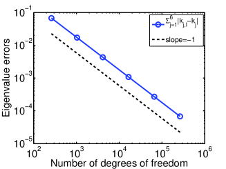
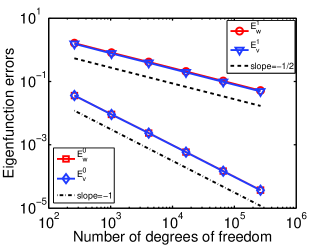
Figure 1: Eigenvalue and eigenfunction errors on the unit disk

Table 1: The first six transmission eigenvalues computed on the unit disk.

$N_{\ell}$	$k_{1,\ell}$	$k_{2,\ell}$	$k_{3,\ell}$	$k_{4,\ell}$	$k_{5,\ell}$	$k_{6,\ell}$
264194	0.7176	0.7176	1.2106	1.2106	1.6841	1.6841

Since the eigenvalues have multiplicity $2$ for $m>0$, we compute the distance to the eigenspaces, i.e.

$$E_{u}^{s}=\sum_{j=1}^{6}\min_{\alpha\in\mathcal{C}^{2}}\left\|u_{j,\ell}-\sum_{i=1}^{2}\alpha_{i}u_{j_{i}}\right\|_{s},\ \ u=w,v,\ s=0,1,$$ (5.4)

where $u_{j_{1}},u_{j_{2}}$ are the corresponding eigenfunctions to the eigenvalue $k_{j}$. The right part of Figure 1 shows the eigenfunction errors versus the number of elements $N_{\ell}$. It is observed that the $H^{1}$-error decreases as $O(N_{\ell}^{-1/2})$ or has the $O(h)$ convergence order, and the $L^{2}$-error decreases as $O(N_{\ell}^{-1})$ or has the $O(h^{2})$ convergence order as implied in Theorem 4.2.

5.2 Transmission eigenvalue problem on the unit square

In this subsection, let $\Omega=(0,1)^{2}$ be the unit square and

$$A(x)=\begin{pmatrix}2+x_{1}^{2}&x_{1}x_{2}\\ x_{1}x_{2}&2+x_{2}^{2}\end{pmatrix},\quad n(x)=4+2(x_{1}+x_{2}).$$

It is easy to verify that the symmetric matrix $A(x)$ and the index of refraction $n(x)$ satisfy the condition (2.2).

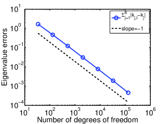
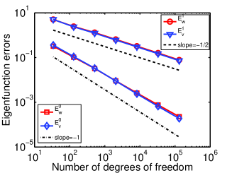
Figure 2: Eigenvalue and eigenfunction errors on the unit square

The quasi-uniform meshes $\{\mathcal{T}_{h_{\ell}}\}_{\ell}$ are used in Algorithm 4.2 to solve the transmission eigenvalue problem. Let $k_{j,l}$ be the $j$-th transmission eigenvalue computed on the mesh $\mathcal{T}_{h_{\ell}}$. In addition, let $k_{j}$ be $j$-th ‘exact’ eigenvalue obtained numerically on a very fine mesh with the number of DOFs $N_{\ell}>10^{6}$. The left part of Figure 2 shows the $\log N_{\ell}$-$\log\sum_{i=1]}^{6}|k_{j,\ell}-k_{j}|$ curve, which again indicates that the sum of the errors for the first six transmission eigenvalues decreases as $O(N_{\ell}^{-1})$ or has the $O(h^{2})$ convergence order. Table 2 depicts the first six transmission eigenvalues computed by Algorithm 4.2 on the mesh with $N_{\ell}=131074$.

Table 2: The first six transmission eigenvalues computed on the unit square.

$N_{\ell}$	$k_{1,\ell}$	$k_{2,\ell}$	$k_{3,\ell}$	$k_{4,\ell}$	$k_{5,\ell}$	$k_{6,\ell}$
131074	1.4808	1.7425	2.3340	3.1636	3.6559	3.7665

The right part of Figure 2 shows the eigenfunction errors

$$E_{u}^{s}=\sum_{j=1}^{6}\|u_{j,\ell}-u_{j}\|_{s},\ \ u=w,v,\ s=0,1.$$ (5.5)

It is also observed that the $H^{1}$-error decreases as $O(N_{\ell}^{-1/2})$ or has the $O(h)$ convergence order, and the $L^{2}$-error decreases as $O(N_{\ell}^{-1})$ or has the $O(h^{2})$ convergence order as implied in Theorem 4.2.

5.3 Transmission eigenvalue problem on the unit square with other conditions on $A(x)$ and $n(x)$

In this subsection, let $\Omega=(0,1)^{2}$ be the unit square. It is stated in Remark 2.1 that our algorithm behaves well if the condition (2.2) is replaced by the condition (2.3). Actually, by using similar arguments, we can also get the convergence results under the condition (2.3). Let

$$A(x)=\begin{pmatrix}\frac{1}{2}+\frac{1}{8}x_{1}^{2}&\frac{1}{8}x_{1}x_{2}\\ \frac{1}{8}x_{1}x_{2}&\frac{1}{2}+\frac{1}{8}x_{2}^{2}\end{pmatrix},\quad n(x)=\frac{1}{4}+\frac{1}{8}(x_{1}+x_{2}).$$

It is easy to verify that the symmetric matrix $A(x)$ and the index of refraction $n(x)$ satisfy the condition (2.3).

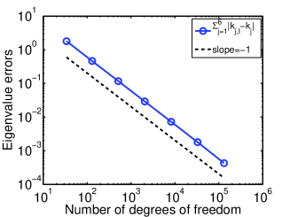
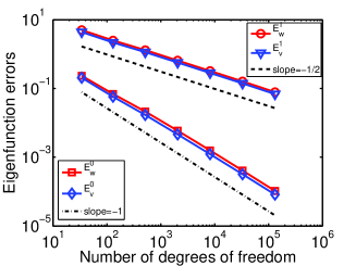
Figure 3: Eigenvalue and eigenfunction errors on the unit square with other conditions on $A(x)$ and $n(x)$

By using the same setting as in the previous subsection, we show the eigenvalue errors and eigenfunction errors in the left part and the right part of Figure 3, respectively. It again demonstrates that the convergence results in Theorem 4.2 is also valid for this kind of coefficient matrix $A(x)$ and the index of refraction $n(x)$. In addition, the first six transmission eigenvalues computed by Algorithm 4.2 are depicted in Table 3.

Table 3: The first six transmission eigenvalues computed on the unit square.

$N_{\ell}$	$k_{1,\ell}$	$k_{2,\ell}$	$k_{3,\ell}$	$k_{4,\ell}$	$k_{5,\ell}$, $k_{6,\ell}$
131074	2.6786	2.7995	3.8921	5.5341	5.8252 $\pm$ 0.8502i

5.4 Transmission eigenvalue problem on the L-shape domain

In this subsection, let $\Omega=(-1,1)^{2}\backslash[0,1)\times(-1,0]$ be the L-shape domain and

$$A(x)=\begin{pmatrix}2+x_{1}^{2}&x_{1}x_{2}\\ x_{1}x_{2}&2+x_{2}^{2}\end{pmatrix},\quad n(x)=2+|x_{1}+x_{2}|.$$

It is easy to verify that the symmetric matrix $A(x)$ and the index of refraction $n(x)$ satisfy the condition (2.2).

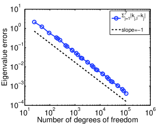
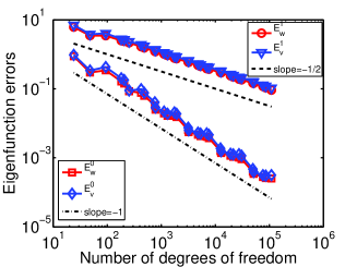
Figure 4: Eigenvalue and eigenfunction errors on the L-shape domain

Since $\Omega$ has reentrant corner, the singularity of the eigenfunctions is expected. We turn to apply the adaptive finite element method for the mesh refinement. Here the ZZ recovery method (c.f. [31]) is adopted as the a posteriori error estimator for eigenfunction and adjoint eigenfunction approximations. Similarly, the ‘exact’ eigenvalues are obtained numerically on a very fine mesh with the number of DOFs $N_{\ell}>10^{6}$.

Figure 4 shows the numerical results for this example. Figure 5 shows the initial mesh and the mesh after $17$ adaptive iterations. It is observed that the multilevel correction method works well on the adaptive meshes and the computational complexity are also quasi-optimal. In addition, Table 4 depicts the first seven transmission eigenvalues computed by Algorithm 4.2 on the mesh with $N_{\ell}=108914$.

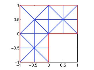
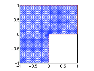
Figure 5: Initial mesh and the mesh after 17 adaptive iterations

Table 4: The first seven transmission eigenvalues computed on the L-shape domain.

$N_{\ell}$	$k_{1,\ell}$	$k_{2,\ell}$	$k_{3,\ell}$	$k_{4,\ell}$	$k_{5,\ell}$	$k_{6,\ell}$, $k_{7,\ell}$
108914	0.8740	1.5895	2.4038	2.6197	2.8764	3.0449 $\pm$ 0.0824i

6 Concluding remarks

In this paper, we give the error estimates for the transmission eigenvalue problem by the finite element method. Furthermore, based on the obtained error estimates in Theorem 3.1, a type of multilevel correction method is proposed to solve the transmission eigenvalue problem. In the multilevel correction method, we transform the transmission eigenvalue solving in the finest finite element space to a sequence of linear problems and some transmission eigenvalue solving in a very low dimensional space. Since the main computational work is to solve the sequence of linear problems, the multilevel correction method can improve the overfull efficiency of the transmission eigenvalue solving. The numerical results also show the efficiency of the proposed numerical scheme.

References