Exactly solvable spin-$1$ Ising-Heisenberg diamond chain with the second-neighbor interaction between nodal spins

Abstract

The spin-1 Ising-Heisenberg diamond chain with the second-neighbor interaction between the nodal spins is rigorously solved using the transfer-matrix method. Exact results for the ground state, magnetization process and specific heat are presented and discussed in particular. It is shown that the further-neighbor interaction between the nodal spins gives rise to three novel ground states with a translationally broken symmetry, but at the same time, it does not increases the total number of intermediate plateaus in a zero-temperature magnetization curve compared with the simplified model without this interaction term. The zero-field specific heat displays interesting thermal dependencies with a single- or double-peak structure.

1 Introduction

The spin-1/2 Ising-Heisenberg diamond chain has received considerable research interest since Čanová et al. [1, 2] reported on first exact results for this interesting quantum spin chain. Early exact results for the spin-1/2 Ising-Heisenberg diamond chain have predicted a lot of intriguing magnetic features such as an intermediate one-third magnetization plateau or double-peak temperature dependencies of specific heat and susceptibility [1, 2]. In spite of a certain over-simplification, the generalized version of the spin-1/2 Ising-Heisenberg diamond chain qualitatively reproduces magnetization, specific heat and susceptibility data reported on the azurite Cu₃(CO₃)₂(OH)₂, which represents the most prominent experimental realization of the spin-1/2 diamond chain [3, 4, 5, 6]. A lot of attention has been therefore paid to a comprehensive analysis of quantum and thermal entanglement [7, 8, 9, 10, 11], correlation functions [12], Lyapunov exponent [13], zeros of partition function [14], magnetocaloric effect [15], the influence of asymmetric [16, 17], further-neighbor [18] and four-spin interactions [19, 20].

Recently, it has been verified that the spin-1 Ising-Heisenberg diamond chain may display more diverse ground states and magnetization curves than its spin-1/2 counterpart [21, 22]. It actually turns out that the magnetization curve of the spin-1 Ising-Heisenberg diamond chain involves intermediate plateaus at zero, one-third and two-thirds of the saturation magnetization even if the relevant ground states do not have translationally broken symmetry [21, 22], while the spin-1/2 Ising-Heisenberg diamond chain may involve those intermediate plateaus just if the asymmetric, further-neighbor [18] and/or four-spin interactions [19, 20] break a translational symmetry of the relevant ground states. In the present work, we aim to examine the role of the second-neighbor interaction between the nodal spins on the ground state and magnetization process of the spin-1 Ising-Heisenberg diamond chain.

The paper is organized as follows. In Sec. 2 we will introduce the investigated spin-chain model and briefly describe basic steps of our rigorous calculation. The most interesting results for the ground state, magnetization process and specific heat are discussed in detail in Sec. 3. Finally, some conclusions and future outlooks are briefly mentioned in Sec. 4.

2 The model and its exact solution

We consider the spin-$1$ Ising-Heisenberg model on a diamond chain in a presence of the external magnetic field. The primitive unit cell of a diamond chain consists of two Heisenberg spins $S_{a,i}$ and $S_{b,i}$, which interact symmetrically via Ising-type interaction with two nearest-neighbor Ising spins $\mu_{i}$ and $\mu_{i+1}$ (see Fig. 1). The total Hamiltonian of the model under investigation may be represented as a sum over block Hamiltonians $\mathcal{H}=\sum_{i=1}^{N}\mathcal{H}_{i}$, where

$$\mathcal{H}_{i} = J[\Delta(S_{a,i}^{x}S_{b,i}^{x}+S_{a,i}^{y}S_{b,i}^{y})+S_{a,i}^{z}S_{b,i}^{z}]+J_{1}\left(S_{a,i}^{z}+S_{b,i}^{z}\right)\left(\mu_{i}+\mu_{i+1}\right)$$ (1)

$$+J_{2}\mu_{i}\mu_{i+1}-H_{\mathrm{H}}\left(S_{a,i}^{z}+S_{b,i}^{z}\right)-H_{\mathrm{I}}\frac{\mu_{i}+\mu_{i+1}}{2}.$$

In above, $S_{a,i}^{\alpha}$ and $S_{b,i}^{\alpha}$ ($\alpha=x,y,z$) denote spatial components of the spin-$1$ operators, $\mu_{i}=\pm 1,0$ stands for the Ising spin, $J$ labels the XXZ interaction between the nearest-neighbor Heisenberg spins, $\Delta$ is a spatial anisotropy in this interaction, $J_{1}$ is the Ising interaction between the nearest-neighbor Ising and Heisenberg spins and finally, the last two terms $H_{\mathrm{H}}$ and $H_{\mathrm{I}}$ determine Zeeman’s energy of the Heisenberg and Ising spins in a longitudinal magnetic field.

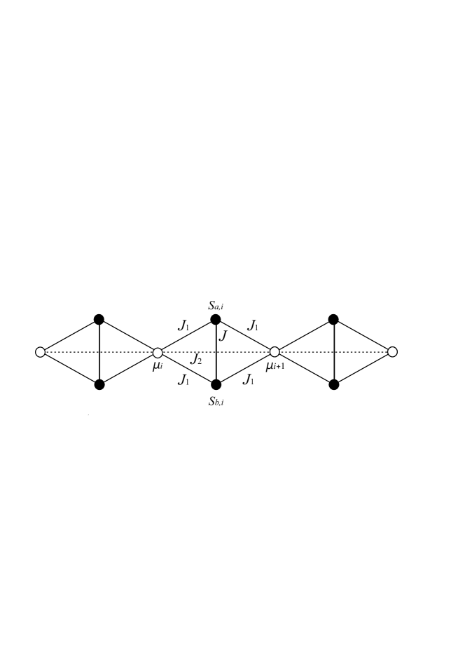
Figure 1: The $i$-th block of the spin-1 diamond chain with the Ising ($\mu_{i}$, $\mu_{i+1}$) and Heisenberg ($S_{a,i}$, $S_{b,i}$) spins.

The important part of our further calculations is based on the commutation relation between different block Hamiltonians $[\mathcal{H}_{i},\mathcal{H}_{j}]=0$, which will allow us to partially factorize the partition function of the model and represent it as a product over block partition functions

$$Z_{N}=\sum_{\{\mu_{i}\}}\prod^{N}_{i=1}\mbox{Tr}_{i}\rm e^{-\beta\mathcal{H}_{i}},$$ (2)

where $\beta=(k_{B}T)^{-1}$, $k_{B}$ is Boltzmann’s constant, $T$ is the absolute temperature, $\sum_{\{\mu_{i}\}}$ marks a summation over spin states of all Ising spins and $\mbox{Tr}_{i}$ means a trace over the spin degrees of freedom of two Heisenberg spins from the $i$-th block. After a straightforward diagonalization of the cell Hamiltonian (1), which corresponds to the spin-1 quantum Heisenberg dimer in a magnetic field, one obtains the following expressions for the respective eigenvalues

$$\mathcal{E}_{1}(\mu_{i},\mu_{i+1}) = -J+J_{2}\mu_{i}\mu_{i+1}-\frac{H_{\rm{I}}}{2}\mu,$$

$$\mathcal{E}_{2,3}(\mu_{i},\mu_{i+1}) = \pm J\Delta+J_{2}\mu_{i}\mu_{i+1}-(J_{1}+\frac{H_{\rm{I}}}{2})\mu+H_{\rm{H}},$$

$$\mathcal{E}_{4,5}(\mu_{i},\mu_{i+1}) = \pm J\Delta+J_{2}\mu_{i}\mu_{i+1}+(J_{1}-\frac{H_{\rm{I}}}{2})\mu-H_{\rm{H}},$$

$$\mathcal{E}_{6,7}(\mu_{i},\mu_{i+1}) = J+J_{2}\mu_{i}\mu_{i+1}+(\pm 2J_{1}-\frac{H_{\rm{I}}}{2})\mu\mp 2H_{\rm{H}},$$

$$\mathcal{E}_{8,9}(\mu_{i},\mu_{i+1}) = -\frac{J}{2}(1\pm\delta)+J_{2}\mu_{i}\mu_{i+1}-\frac{H_{\rm{I}}}{2}\mu,$$ (3)

where $\mu\equiv\mu_{i}+\mu_{i+1}$ and $\delta=\sqrt{1+8\Delta^{2}}$. Now, one may simply perform a trace over the spin degrees of freedom of the spin-1 Heisenberg dimers on the right-hand-side of Eq. (2) and the partition function can be consequently rewritten into the following form

$$Z_{N}=\sum_{\{\mu_{i}\}}\prod^{N}_{i=1}T_{\mu_{i},\mu_{i+1}}=\mbox{Tr}\,T^{N},$$ (4)

where the expression $T_{\mu_{i},\mu_{i+1}}$ can be viewed the standard $3\times 3$ transfer matrix

$$T_{\mu_{i},\mu_{i+1}}=\left(\begin{array}[]{cccc}T_{1,1}&T_{1,0}&T_{1,-1}\\ \ T_{0,1}&T_{0,0}&T_{0,-1}\\ \ T_{-1,1}&T_{-1,0}&T_{-1,-1}\end{array}\right).$$ (8)

Here, the subscripts $\pm 1$ and 0 denote three available spin states of the Ising spins $\mu_{i}$ and $\mu_{i+1}$ involved in the transfer matrix (8), which has precisely the same form as the transfer matrix of the generalized spin-1 Blume-Emery-Griffiths chain diagonalized in Refs. [23, 24, 25]. Of course, individual elements of the transfer matrix (8) are defined through the formula

$$T_{\mu_{i},\mu_{i+1}}=\mbox{Tr}_{i}\rm e^{-\beta\mathcal{H}_{i}}=\sum_{n=1}^{9}\rm e^{-\beta\mathcal{E}_{n}(\mu_{i},\mu_{i+1})},$$ (9)

which includes the set of eigenvalues (3) for the spin-1 quantum Heisenberg dimer and can be rewritten as

$$T_{\mu_{i},\mu_{i+1}}=\mathrm{exp}(-\beta J_{2}\mu_{i}\mu_{i+1}+\beta H_{\rm{I}}\mu/2)[2\mathrm{exp}(\beta J/2)\mathrm{cosh}(\beta J\delta/2)+\mathrm{exp}(\beta J)$$

$$+4\mathrm{cosh}(\beta J\Delta)\mathrm{cosh}(\beta J_{1}\mu-\beta H_{\rm{H}})+2\mathrm{exp}(-\beta J)\mathrm{cosh}(2\beta J_{1}\mu-2\beta H_{\rm{H}})].$$ (10)

With regard to Eq. (4), the partition function of the spin-1 Ising-Heisenberg diamond chain can be expressed through three eigenvalues of the transfer matrix [23, 24]

$$Z_{N}=\lambda_{1}^{N}+\lambda_{2}^{N}+\lambda_{3}^{N},$$ (11)

which can be evaluated from

$$\lambda_{k}=\frac{1}{3}\left(u_{k}g+\frac{a^{2}-3b}{u_{k}g}-a\right).$$ (12)

The coefficients $u_{k}$, $g$, $a$, $b$ and $c$ entering the eigenvalues (12) are given by $\\ u_{1}=1,u_{2,3}=(-1\pm i\sqrt{3})/2,\\ g=2^{-1/3}(9ab-2a^{3}-27c+3\sqrt{3}\sqrt{4b^{3}-a^{2}b^{2}+4a^{3}c-18abc+27c^{2}})^{1/3},\\ a=-T_{1,1}-T_{0,0}-T_{-1,-1},\\ b=-T_{1,0}^{2}-T_{1,-1}^{2}-T_{-1,0}^{2}+T_{1,1}T_{0,0}+T_{1,1}T_{-1,-1}+T_{0,0}T_{-1,-1},\\ c=-2T_{1,0}T_{1,-1}T_{-1,0}+T_{1,1}T_{-1,0}^{2}+T_{1,-1}^{2}T_{0,0}+T_{1,0}^{2}T_{-1,-1}-T_{1,1}T_{0,0}T_{-1,-1}.$

Next, let us denote the largest transfer-matrix eigenvalue $\lambda=\mbox{max}\{\lambda_{1},\lambda_{2},\lambda_{3}\}$, because the contribution of two smaller transfer-matrix eigenvalues to the partition function may be completely neglected in the thermodynamic limit $N\rightarrow\infty$

$$Z_{N}\simeq\lambda^{N}.$$ (13)

The free energy per elementary diamond cell can be obtained from the largest eigenvalue of the transfer matrix (9) according to the formula

$$f=-\frac{1}{\beta}\lim_{N\to\infty}\frac{1}{N}\ln Z_{N}=-\frac{1}{\beta}\ln\lambda.$$ (14)

Knowledge of the free energy allows us to obtain thermodynamic quantities of the system (such as entropy, magnetization, specific heat, etc.) in terms of the free energy and/or its derivatives. In particular, for the entropy $s$ and the heat capacity $c$ per unit cell one can obtain

$$s=k_{B}\beta^{2}\frac{\partial f}{\partial\beta},\quad c=-\beta\frac{\partial s}{\partial\beta}.$$ (15)

One may also obtain the single-site magnetization of the Ising ($m_{\mathrm{I}}=\langle\mu_{i}+\mu_{i+1}\rangle/2$) and the Heisenberg ($m_{\mathrm{H}}=\langle S_{a,i}^{z}+S_{b,i}^{z}\rangle/2$) spins, which are given by

$$m_{\mathrm{I}}=-\frac{\partial f}{\partial H_{\mathrm{I}}},\quad m_{\mathrm{H}}=-\frac{\partial f}{\partial H_{\mathrm{H}}}.$$ (16)

Finally, the total magnetization per site follows from

$$m=\frac{1}{3}m_{\mathrm{I}}+\frac{2}{3}m_{\mathrm{H}}.$$ (17)

3 Results and discussion

In this section, we will investigate in detail the ground state, magnetization process and specific heat of the spin-1 Ising-Heisenberg diamond chain with antiferromagnetic coupling constants $J>0$ and $J_{1}>0$. Hereafter, we will consider for simplicity the uniform external magnetic field acting on the Ising and Heisenberg spins $H_{\mathrm{H}}=H_{\mathrm{I}}\equiv H$. Again for simplicity, the Boltzmann’s constant is set to unity $k_{B}=1$ and a strength of the Ising coupling $J_{1}$ will be subsequently used for introducing a set of dimensionless parameters

$$\alpha=\frac{J}{J_{1}},\quad\gamma=\frac{J_{2}}{J_{1}},\quad h=\frac{H}{J_{1}},\quad t=\frac{T}{J_{1}},$$ (18)

which determine a relative strength of the Heisenberg coupling, the second-neighbor interaction between the nodal spins, the magnetic field and temperature, respectively. The spin-1 Ising-Heisenberg diamond chain without the second-neighbor interaction between the nodal spins was studied in some detail in our previous work [21], so our particular attention will be primarily devoted to the effect of this interaction term.

Let us at first consider the ground-state phase diagrams of the spin-1 Ising-Heisenberg diamond chain in zero and non-zero magnetic field. Depending on a relative strength of the second-neighbor interaction $\gamma$ only two or three different ground states are available at zero magnetic field: the classical ferrimagnetic (FRI) phase and two quantum antiferromagnetic ones QAF₁ and QAF₂. The three aforementioned phases can be characterized by the following eigenvectors, the ground-state energy and single-site magnetizations:

• The classical ferrimagnetic phase FRI:

  $$|FRI\rangle=\prod^{N}_{i=1}|-1\rangle_{i}\otimes|1,1\rangle_{a_{i},b_{i}},$$

  $$E=J+J_{2}-4J_{1}-H,m_{\mathrm{I}}=-1,m_{\mathrm{H}}=1,m=1/3.$$ (19)

• The quantum antiferromagnetic phases QAF₁ and QAF₂:

  $$|QAF_{1}\rangle=\left\{\begin{array}[]{l}\displaystyle\prod^{N}_{i=1}|1\rangle_{i}\otimes\frac{1}{\sqrt{2}}(|0,-1\rangle-|-1,0\rangle)_{a_{i},b_{i}},\\ \displaystyle\prod^{N}_{i=1}|-1\rangle_{i}\otimes\frac{1}{\sqrt{2}}(|1,0\rangle-|0,1\rangle)_{a_{i},b_{i}},\end{array}\right.$$ (22)

  $$E=-J\Delta+J_{2}-2J_{1},m_{\mathrm{I}}=\pm 1,m_{\mathrm{H}}=\mp 0.5,m=0,$$

  $$|QAF_{2}\rangle=\prod^{N}_{i=1}|(-1)^{i}\mathrm{or}(-1)^{i+1}\rangle_{i}\otimes\frac{\Delta\sqrt{2}}{\sqrt{\delta(\delta-1)}}(\frac{1-\delta}{2\Delta}|0,0\rangle$$

  $$+|1,-1\rangle+|-1,1\rangle)_{a_{i},b_{i}},$$

  $$E=-\frac{J}{2}(1+\delta)-J_{2},m_{\mathrm{I}}=0,m_{\mathrm{H}}=0,m=0.$$ (23)

The zero-field ground-state phase diagram of the spin-1 Ising-Heisenberg diamond chain is plotted in Fig. 2(a) in $\Delta-\alpha$ plane for two different values of the second-neighbor interaction $\gamma$. Note that an increase of the Heisenberg coupling $\alpha$ strengthens a spin frustration due to a competition between the antiferromagnetic Heisenberg and Ising interactions. If the second-neighbor interaction between the nodal spins is sufficiently small (e.g. $\gamma=0.2$), then, one passes from FRI ground state through QAF₁ ground state up to QAF₂ ground state as the frustration parameter $\alpha$ strengthens. On the other hand, QAF₁ ground state without translationally broken symmetry is totally absent in the ground-state phase diagram for strong enough second-neighbor interaction (e.g. $\gamma=0.75$).

(a)	(b)
(c)	(d)

Figure 2: (a) Zero-field ground-state phase diagram in the $\Delta-\alpha$ plane for a few different values of the interaction parameter $\gamma$; (b)-(d) Ground-state phase diagrams in the $\alpha-h$ plane for a fixed value of the anisotropy parameter $\Delta=1$ and a few selected values of the second-neighbor interaction: (b) $\gamma=0,\gamma=0.2$, (c) $\gamma=1/3,\gamma=0.5$ and (d) $\gamma=0.75,\gamma=1$.

In a presence of the external magnetic field one may additionally find another five ground states of the spin-1 Ising-Heisenberg diamond chain: three quantum ferromagnetic (QFO₁, QFO₂, QFO₃), the unsaturated ferromagnetic (UFM) and the saturated paramagnetic (SPA), which can be characterized through the following eigenvectors, the ground-state energy and single-site magnetizations:

• The quantum ferromagnetic phases QFO₁, QFO₂ and QFO₃:

  $$|QFO_{1}\rangle=\prod^{N}_{i=1}|1\rangle_{i}\otimes\frac{1}{\sqrt{2}}(|1,0\rangle-|0,1\rangle)_{a_{i},b_{i}},$$

  $$E=-J\Delta+2J_{1}+J_{2}-2H,m_{\mathrm{I}}=1,m_{\mathrm{H}}=1/2,m=2/3,$$

  $$|QFO_{2}\rangle=\prod^{N}_{i=1}|1\rangle_{i}\otimes\frac{\Delta\sqrt{2}}{\sqrt{\delta(\delta-1)}}(\frac{1-\delta}{2\Delta}|0,0\rangle+|1,-1\rangle+|-1,1\rangle)_{a_{i},b_{i}},$$

  $$E=-\frac{J}{2}(1+\delta)+J_{2}-H,m_{\mathrm{I}}=1,m_{\mathrm{H}}=0,m=1/3,$$

  $$|QFO_{3}\rangle=\prod^{N}_{i=1}|(-1)^{i}\mathrm{or}(-1)^{i+1}\rangle_{i}\otimes\frac{1}{\sqrt{2}}(|1,0\rangle-|0,1\rangle)_{a_{i},b_{i}},$$

  $$E=-J\Delta-J_{2}-H,m_{\mathrm{I}}=0,m_{\mathrm{H}}=1/2,m=1/3.$$ (24)

• The unsaturated ferromagnetic phase UFM:

  $$|UFM\rangle=\prod^{N}_{i=1}|(-1)^{i}\mathrm{or}(-1)^{i+1}\rangle_{i}\otimes|1,1\rangle_{a_{i},b_{i}},$$

  $$E=J-J_{2}-2H,m_{\mathrm{I}}=0,m_{\mathrm{H}}=1,m=2/3.$$ (25)

• The saturated paramagnetic phase SPA:

  $$|SPA\rangle=\prod^{N}_{i=1}|1\rangle_{i}\otimes|1,1\rangle_{a_{i},b_{i}},$$

  $$E=J+4J_{1}+J_{2}-3H,\;m_{\mathrm{I}}=1,m_{\mathrm{H}}=1,m=1.$$ (26)

The ground-state phase diagram of the spin-1 Ising-Heisenberg diamond chain in $\alpha-h$ plane is plotted in Fig. 2(b)-(d) for the isotropic Heisenberg coupling $\Delta=1$ and several values of the second-neighbor interaction $\gamma$. It can be seen from Fig. 2(b) that the second-neighbor interaction between the nodal spins gives rise to two new ground states QAF₂ and UFM, which are absent in the model without this interaction term. In general, the parameter space inherent to the ground states QAF₂ and UFM extends upon rising the second-neighbor interaction $\gamma$ as evidenced by from Fig. 2(b) and (c). However, the third novel ground state QFO₃ appears at moderate values of the Heisenberg coupling $\alpha$ and magnetic field $h$ as far as the second-neighbor interaction $\gamma$ becomes sufficiently strong (see Fig. 2(d)).

Now, let us proceed to a comprehensive analysis of the magnetization process at zero as well as non-zero temperatures. To illustrate an influence of the second-neighbor coupling on a magnetization process, Figs. 3(a) and 4(a) compare two different magnetization scenarios of the spin-1 Ising-Heisenberg diamond chain with and without this interaction term. Fig. 3(a) displays the magnetization curve with a single one-third plateau due to a field-induced transition FRI-SPA for $\gamma=0$ along with the magnetization curve with two successive one-third and two-thirds plateaus, which emerge due to two subsequent field-induced transitions FRI-UFM-SPA for $\gamma=1/3$. Interestingly, the simple magnetization curve with a single one-third plateau due to a field-induced transition FRI-SPA for $\gamma=0$ may also change to a more complex magnetization curve with three successive plateaus at zero, one-third and two-thirds of the saturation magnetization, which emerge due to three subsequent field-induced transitions QAF₂-FRI-UFM-SPA for $\gamma=1$. It is worthwhile to recall that actual magnetization plateaus and magnetization jumps only appear at zero temperature, while increasing temperature gradually smoothens the magnetization curves. Typical thermal variations of the total magnetization are plotted Figs. 3(b) and 4(b), which evidence pronounced low-temperature variations of the total magnetization when the magnetic field is fixed slightly below or above the relevant critical field.

(a)	(b)

Figure 3: (a) The total magnetization as a function of the magnetic field at a few different temperatures for the isotropic Heisenberg interaction ($\Delta=1$) of a relative strength $\alpha=0.5$. The dotted and solid lines show magnetization curves for two selected values of the second-neighbor interaction $\gamma=0$ and $1/3$, respectively. (b) Thermal variations of the total magnetization for $\Delta=1$, $\alpha=0.5$, $\gamma=1/3$ and several values of the external magnetic field.

(a)	(b)

Figure 4: (a) The total magnetization as a function of the magnetic field at a few different temperatures for the isotropic Heisenberg interaction ($\Delta=1$) of a relative strength $\alpha=0.9$. The dotted and solid lines show magnetization curves for two selected values of the second-neighbor interaction $\gamma=0$ and $1$, respectively. (b) Thermal variations of the total magnetization for $\Delta=1$, $\alpha=0.9$, $\gamma=1$ and several values of the external magnetic field.

Last but not least, let us briefly comment on thermal variations of the zero-field specific heat, which are quite typical for three available zero-field ground states FRI, QAF₁ and QAF₂. Temperature dependencies of the zero-field specific heat pertinent to the classical FRI ground state are depicted in Fig. 5(a). It can be seen from this figure that the specific heat may display a more peculiar double-peak temperature dependence in addition to a standard temperature dependence with a single round maximum. The double-peak temperature dependencies of the specific heat are also quite typical for another ground state QAF₁, which appears in a rather restricted region of parameter space (see Fig. 5(b)). On assumption that the QAF₂ phase constitutes the ground state thermal variations of the zero-field specific heat with a single- or double-peak structure emerge for greater or smaller values of the Heisenberg interaction $\alpha$ as depicted in Fig. 5(c). It could be concluded that the double-peak temperature dependencies of the specific heat appear in all three aforementioned cases owing to low-lying thermal excitations and consequently, the low-temperature peak can be always identified as the Schottky-type maximum.

(a)	(b)
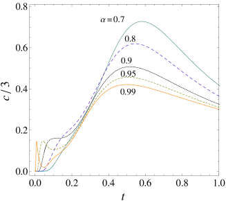
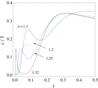
(c)

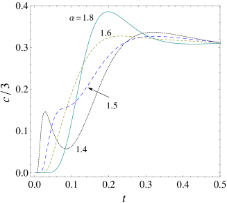
Figure 5: Typical temperature dependences of the zero-field specific heat for the fixed value of the second-neighbor interaction $\gamma=1/3$ and a few different values of the isotropic Heisenberg coupling with $\Delta=1$. Three panels correspond to three available zero-field ground states: (a) FRI, (b) QAF₁ and (c) QAF₂.

4 Conclusion

In the present work, we have examined the ground state, magnetization process and specific heat of the exactly solved spin-$1$ Ising-Heisenberg diamond chain with the second-neighbor interaction between the nodal spins. It has been demonstrated that the considered further-neighbor interaction gives rise to three novel ground states, which cannot be in principle detected in the simplified version of the spin-$1$ Ising-Heisenberg diamond chain without this interaction term [21]. It should be pointed out, moreover, that the spin-$1$ Ising-Heisenberg diamond chain supplemented with the second-neighbor interaction between the nodal spins does not exhibit more intermediate magnetization plateaus than its simplified version without this interaction term even though all three novel ground states have translationally broken symmetry. This finding seems to be quite surprising, because one could generally expect according to Oshikawa-Yamanaka-Affleck rule [26, 27] appearance of new intermediate plateaus at one-sixth and five-sixths of the saturation magnetization in addition to the observed intermediate plateaus at zero, one-third and two-thirds of the saturation magnetization. Of course, one cannot definitely rule out that the one-sixth and/or five-sixths plateaus indeed occur in a zero-temperature magnetization curve of a more general spin-$1$ Ising-Heisenberg diamond chain, which could for instance take into account asymmetric interactions, single-ion anisotropy, four-spin and/or biquadratic interactions besides the second-neighbor interaction between the nodal spins. This conjecture might represent challenging task for future investigations.

References

References

- [1] L. Čanová, J. Strečka, M. Jaščur, Czech. J. Phys. 54 (2004) D579.
- [2] L. Čanová, J. Strečka, M. Jaščur, J. Phys.: Condens. Matter 18 (2006) 4967.
- [3] H. Kikuchi, Y. Fujii, M. Chiba, S. Mitsudo, T. Idehara, Physica B 329-333 (2003) 967.
- [4] H. Kikuchi, Y. Fujii, M. Chiba, S. Mitsudo, T. Idehara, T Kuwai, J. Magn. Magn. Mater. 272 276 (2004) 900.
- [5] H. Kikuchi, Y. Fujii, M. Chiba, S. Mitsudo, T. Idehara, T. Tonegawa, K. Okamoto, T. Sakai, T. Kuwai, H. Ohta, Phys. Rev. Lett. 94 (2005) 227201.
- [6] H. Kikuchi, Y. Fujii, M. Chiba, S. Mitsudo, T. Idehara, T. Tonegawa, K. Okamoto, T. Sakai, T. Kuwai, K. Kindo, A. Matsuo, W. Higemoto, K. Nishiyama, M. Horvatic, C. Bertheir, Prog. Theor. Phys. Suppl. 159 (2005) 1.
- [7] N.S. Ananikian, L.N. Ananikyan, L.A. Chakhmakhchyan, O. Rojas, J. Phys.: Condens. Matter 24 (2012) 256001.
- [8] O. Rojas, M. Rojas, N.S. Ananikian, S.M. de Souza, Phys. Rev. A 86 (2012) 042330.
- [9] J. Torrico, M. Rojas, S.M. de Souza, O. Rojas, N.S. Ananikian, EPL 108 (2014) 50007.
- [10] E. Faizi, H. Eftekhari, Rep. Math. Phys. 74 (2014) 251.
- [11] E. Faizi, H. Eftekhari, Chin. Phys. Lett. 32 (2015) 100303.
- [12] S. Bellucci, V. Ohanyan, Eur. Phys. J. B 86 (2013) 446.
- [13] N. Ananikian, V. Hovhannisyan, Physica A 392 (2013) 2375.
- [14] N.S. Ananikian, V. Hovhannisyan, R. Kenna, Physica A 396 (2014) 51.
- [15] Y. Qi, A. Du, Phys. Status Solidi B 251 (2014) 1096.
- [16] J.S. Valverde, O. Rojas, S.M. de Souza, J. Phys.: Condens. Matter 20 (2008) 345208.
- [17] B.M. Lisnii, Ukr. J. Phys. 56 (2011) 1237.
- [18] B.M. Lisnyi, J. Strečka, Phys. Status Solidi B 251 (2014) 1083.
- [19] L. Gálisová, Phys. Status Solidi B 250 (2013) 187.
- [20] L. Gálisová, Condens. Matter Phys. 17 (2014) 13001.
- [21] N.S. Ananikian, J. Strečka, V. Hovhannisyan, Solid St. Commun. 194 (2014) 48.
- [22] V.S. Abgaryan, N.S. Ananikian, L.N. Ananikyan, V.V. Hovhannisyan, Solid St. Commun. 224 (2015) 15.
- [23] S. Krinsky, D. Furman, Phys. Rev. Lett. 32 (1974) 731.
- [24] S. Krinsky, D. Furman, Phys. Rev. B 11 (1975) 2602.
- [25] B. Lisnyi, J. Strečka, J. Magn. Magn. Mater. 46 (2013) 78.
- [26] M. Oshikawa, M. Yamanaka, I. Affleck, Phys. Rev. Lett. 78 (1997) 1984.
- [27] I. Affleck, Phys. Rev. B 37 (1998) 5186.