On the behaviour of streams in angle and frequency spaces in different potentials

We have studied the behaviour of stellar streams in the Aquarius fully cosmological N-body simulations of the formation of Milky Way halos. In particular, we have characterised the streams in angle and frequency spaces derived using an approximate but generally well-fitting spherical potential. We have also run several test-particle simulations to understand and guide our interpretation of the different features we see in the Aquarius streams. Our goal is both to establish which deviations of the expected action-angle behaviour of streams exist because of the approximations made on the potential, but also to derive to what degree we can use these coordinates to model streams reliably.
We have found that many of the Aquarius streams wrap in angle space along relatively straight lines, and distribute themselves along linear structures also in frequency space. On the other hand, from our controlled simulations we have been able to establish that deviations from spherical symmetry, the use of incorrect potentials and the inclusion of self-gravity lead to streams in angle space to still be along relatively straight lines but also to depict wiggly behaviour whose amplitude increases as the approximation to the true potential becomes worse. In frequency space streams typically become thicker and somewhat distorted. Therefore, our analysis explains most of the features seen in the approximate angle and frequency spaces for the Aquarius streams with the exception of their somewhat ‘noisy’ and ‘patchy’ morphologies. These are likely due to the interactions with the large number of dark matter subhalos present in the cosmological simulations. Since the measured angle-frequency misalignments of the Aquarius streams can largely be attributed to using the wrong (spherical) potential, the determination of the mass growth history of these halos will only be feasible once (and if) the true potential has been determined robustly.

1 Introduction

In the last two decades much progress has been made on the discovery and characterisation of tidal streams around our Milky Way and in other nearby galaxies (see e.g. Koposov et al. 2012; Martin et al. 2014). Tidal streams consist of stars stripped from satellites (dwarf galaxies and globular clusters) that move on nearby almost parallel orbits. As such they constitute extremely sensitive probes of the mass distribution in the host system (Johnston et al. 1999; Ibata et al. 2001; Johnston & Bullock 2004; Law et al. 2005; Law & Majewski 2010; Koposov et al. 2010; Vera-Ciro & Helmi 2013; Sanders & Binney 2013b; Sanderson et al. 2014). This is one of the drivers of the observational and theoretical studies of streams, as one of the ultimate goals is to establish the mass distribution in the dark halo of galaxies like the Milky Way, which in turn will lead to a better understanding of the nature of dark matter (see e.g. Strigari 2013).

The recently launched Gaia satellite (Perryman et al. 2001) will provide the phase-space coordinates of a vast sample of stars in the Milky Way in the next decade. Together with spectroscopic follow-up surveys of the fainter Gaia stars such as 4MOST (de Jong et al. 2012) and WEAVE (Dalton et al. 2012), these datasets will provide an unprecedented detailed view of our Galaxy. Our understanding of the dynamics of the halo and its streams needs to be sharpened to maximally exploit the wealth of data that will soon become available (see e.g. Johnston et al. 1999; Law & Majewski 2010; Eyre & Binney 2011; Bonaca et al. 2014).

Action-angle coordinates provide an excellent tool to describe the evolution of streams (Tremaine 1999; Helmi & White 1999). For example, the evolution of stars in angle space is linear with time for a static potential, while the actions are adiabatic invariants. The difficulty lies in finding the necessary coordinate transformations to map observables into action-angle space. Only for specific types of potentials, including spherical and those of Staeckel form, can we directly compute the angles and actions because the Hamilton-Jacobi equation is separable (Goldstein 1950; de Zeeuw 1985; Binney & Tremaine 2008). However, in recent years several approximate schemes have been developed to overcome this problem. For example, an appropriate toy potential can be used to compute the true action-angles, based on the work of McGill & Binney (1990) and Kaasalainen & Binney (1994) (see e.g. McMillan & Binney 2008; Fox 2012; Sanders & Binney 2014; Bovy 2014). Another method is to approximate the potential locally by a Staeckel potential (axisymmetric or triaxial), a procedure known as the ‘Staeckel fudge’ (Binney 2012; Sanders & Binney 2015).

Figure 1: The enclosed mass (left) and circular velocity (right) for halo Aq-A (top panels) and halo Aq-D (bottom panels) with NFW fits to the circular velocity (blue lines). The red dashed curve shows the profile when we match the peak velocity. For an NFW the position of this maximum depends only on $r_{\textrm{s}}$ and its magnitude only on $M_{\textrm{s}}$. The radial range plotted starts at the convergence radius (Power et al. 2003; Navarro et al. 2010) and extends up to $r_{200}$ (see Springel et al. 2008).

The availability of full phase-space information for a large number of stars in the Gaia dataset will assist greatly in exploiting the power of action-angle coordinates for streams (McMillan & Binney 2008; Gómez et al. 2010). Actions (and integrals of motion) may be used as well to derive the accretion history of the halo of the Milky Way, because even when a stream is fully phase mixed it is still clumped in this space (Helmi & de Zeeuw 2000; also see Gómez & Helmi 2010). We do require the potential to evolve adiabatically slowly for the actions to remain clumped. This clumpiness in action space can also be employed to determine the gravitational field in which the stars have evolved because the largest degree of clustering occurs when the actions are computed in the true potential (Sanderson et al. 2014; Magorrian 2014; Peñarrubia et al. 2012). The angles and frequencies can also be used to this end, because streams should lie along straight lines that have the same slope in angle and in frequency space for the correct gravitational potential under the condition that it is static (Sanders & Binney 2013a, b). In Buist & Helmi (2015) we argued that an adiabatically growing potential will cause a small difference in these slopes, or an “angle-frequency misalignment”. We also pointed out that in angle and frequency space there are several other indicators that the potential used in the computation may be incorrect. This will allow the determination of the characteristic parameters of the true potential to be separated from its time-evolution.

We continue along that line of study in this Paper, where we explore the behaviour of streams evolved in fully cosmological N-body simulations. In particular, we characterise the streams in the angle and frequency spaces obtained using an approximate spherical potential. We also run several test-particle simulations to understand and guide our interpretation of the different features we see in the cosmological simulations. Our goal is both to establish which perturbations of the action-angle behaviour of streams exist because of the approximations made on the potential, but also to derive to which degree we can use these coordinates to study cosmologically evolved streams.

The structure of this Paper is as follows. In Sec. 2 we describe the cosmological N-body simulations and the stream catalogue used. In Sec. 3 we discuss their behaviour in action-angle coordinates, computed using an appropriately chosen spherical potential. To guide our understanding of the behaviour of these streams we present in Sec. 4 a set of test-particle streams evolved in an axisymmetric potential, loosely based on the cosmological simulations. In Sec. 5 we gain further insight into the generic behaviour of streams by determining the impact of computing the action-angles of the test-particle simulations of Sec. 4 in several incorrect potentials, and discuss the effect of self-gravity. We end in Sec. 6 with a discussion and conclusions.

2 Streams in cosmological simulations

2.1 Description of the Aquarius project and its stellar halos

The Aquarius project (Springel et al. 2008; Navarro et al. 2010) consists of a set of six re-simulations of Milky-Way mass ($\sim 10^{12}\textrm{ M}_{\odot}$) dark matter halos extracted from a larger cosmological parent simulation (Boylan-Kolchin et al. 2009). They were selected to have no close massive neighbours at $z=0$, and form late-type galaxies when evolved using semi-analytic galaxy formation models. Halos Aq-A to Aq-E are believed to be representative of the Milky Way, while Aq-F experiences a recent major merger and hence is less suitable (Wang et al. 2011). We focus our study of streams to two of the halos, Aq-A and Aq-D to avoid flooding this article with examples while providing a flavour of the variations found in different systems.

We extract streams from the accreted component of stellar halos modelled using the Durham semi-analytic model GALFORM. Cooper et al. (2010) have associated stellar populations with dark matter particles in the simulations via a ‘tagging’ scheme. Lowing et al. (2015) took this a step further and generated individual stars from these populations by re-sampling the dark matter particles and using stellar population synthesis modelling. Another difference between these works is that Cooper et al. used the Bower et al. (2006) version of GALFORM, while Lowing et al. used the Font et al. (2011) version which has improved physics on dwarf galaxy scales that makes model satellites more similar to those observed around the Milky Way. Here we use the public catalogue that Lowing et al. offer online, which has all stars with magnitude $M_{g}<7$.

The Lowing dataset re-samples the dark matter particle positions and velocities in a way that aims to preserve their distribution in phase-space. To observe streams in the halo of the Milky Way it is common to select the Red Giant Branch (RGB) stars because they are intrinsically bright. We noticed that some of the thinner simulated streams look quite clumpy when only using the RGB stars, most likely because of the re-sampling of the dark matter particles. Since our interest is only in the dynamical features of the streams, we instead decided to use the source (‘tagged’) dark matter particles. To this end we have matched the dark matter ID’s to those in the outputs of the Aquarius simulations and found the positions and velocities of the source particles from the Lowing dataset. Whether we would have used the RGB stars or the dark matter particles does not matter much for the number statistics as both sets have similar sizes.

We aligned the coordinate system to that of the parent dark halo by using the principal axes determined at 100 kpc from the centre by Vera-Ciro et al. (2011). These authors used the reduced inertia tensor method (Allgood et al. 2006) which closely follows isodensity contours. The $z$-direction is set along the major axis of these halos. Further details on the shapes are discussed in Sec. 4.1.

2.2 Mass distribution of the Aquarius halos

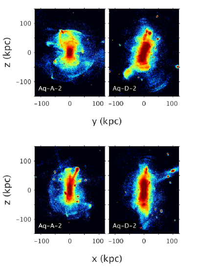
Figure 2: Density maps of all the dark matter particles tagged with stellar populations originating in objects in halos Aq-A and Aq-D with more than 500 dark matter particles in their progenitor. The coordinate system is aligned with the principal axes of the halo at 100 kpc. The minor and intermediate axes are in the $x$-$y$ plane and the major axis is along the $z$ direction.

Although intrinsically triaxial, with triaxiality parameters in the range 2/3 to 1 (see Sec. 4.1), the Aquarius halos can be fit reasonably well with a spherical mass profile. Here we use Navarro-Frenk-White functional form (Navarro et al. 1996, 1997, hereafter NFW), which provides a relatively good description in the regions where we study streams ($r\sim 50-100$ kpc, see Springel et al. 2008; Navarro et al. 2010), and we prefer it because of its simplicity and computational efficiency compared to the slightly better fitting Einasto profile (Einasto 1965).

In Fig. 1 we show the results obtained when fitting the spherically averaged circular velocity profile with two free parameters, the scale mass $M_{\textrm{s}}$ and the scale radius $r_{\textrm{s}}$, for halo Aq-A and halo Aq-D (see also Navarro et al. 2010). The scale mass is defined as $M_{\textrm{s}}=M(r_{\textrm{s}})$ and is related to the virial mass as

$$M_{\textrm{s}}=\frac{M_{\textrm{vir}}}{f(c)};\ \ f(x)=\frac{\log(1+x)-x/(1+x)}{\log(2)-1/2},$$ (1)

where the concentration $c\equiv r_{\textrm{vir}}/r_{\textrm{s}}$. Note that halo Aq-D is much better fitted by an NFW profile than halo Aq-A, which appears to have a bump in its circular velocity profile. Aq-A is also more triaxial than Aq-D (Vera-Ciro et al. 2011).

2.3 Selection of streams

Not all objects in the Aquarius stellar halos are apparent as stream-like structures, for example this may be the case if the object is too small or if it has not been significantly disrupted. Fig. 2 shows that large streamy structures exist out to large radii (see also Cooper et al. 2010). Each of the 2 Aquarius stellar halos have of the order of 100-200 individual progenitors, of which about 20% have produced discernible stream-like features by $z=0$, for example, a visible piece of a loop. We selected these by eye in physical space and verified this selection by checking that they also appeared streamy in their approximate angle coordinates, as discussed later. For comparison we also included several massive and seemingly phase mixed objects that most likely represent debris on quite radial orbits. We also impose a lower limit of at least 500 ‘tagged’ dark matter particles for each progenitor to exclude the really small streams. This corresponds to a ‘tagged’ dark matter mass of $\sim 7\times 10^{6}\textrm{ M}_{\odot}$, and yields a total of 35 streams for halo Aq-A and Aq-D together. In the main part of this Paper we focus on 10 streams from each halo to illustrate their behaviour, a selection which includes a few of the highly phase-mixed shell-like structures that appear near the long axis (here the $z$-axis) and which move on more radial orbits. The remaining 25 streams are shown in the Appendix.

2.4 The morphology of selected streams

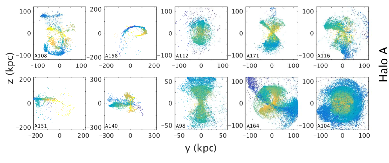
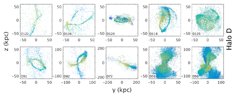
Figure 3: Stream-like objects in Aq-A (top) and Aq-D (bottom) in the same projection as in the top panel of Fig. 2. Shown here are the ‘tagged’ dark matter particles while the labels indicate the object IDs used throughout this Paper. The ranges are different in each panel to show the streams in maximum detail. The colours represent the energy gradient computed using the best-fitting spherical NFW potential, with yellow the most bound particles, and blue those least bound. The streams have been sorted by dark matter mass, with the lightest stream on the top-left and the most massive on the bottom-right.

Streams consist of groups of stars that have similar orbits, and the relatively small variance in their orbits creates structures whose trajectory follows closely the orbit of the progenitor (Jin & Lynden-Bell 2007; Binney 2008), although not exactly (Choi et al. 2007; Eyre & Binney 2009; Sanders & Binney 2013b). We can therefore analyse the streams in terms of the orbits permitted by the potential.

Our selection of individual streams for halo Aq-A and Aq-D are shown in Fig. 3. To some extent, the consideration of structures in these two different haloes help us gauge the variety and similarities in the characteristics of their streams. The IDs of the streams given in this figure correspond one-to-one with tree-IDs in the Lowing catalogue. We provide the progenitor’s masses of these streams in Appendix A. The colours in the figure represent the binding energy computed in the best fitting spherical NFW potential (yellow is the most bound, blue is the least bound). Most of the streams depict at least one clear stream-like feature or loop (almost by construction, and for as far as a 2-D projection allows us to show this), except for the debris for A98, A104, D56 and D98, which we selected to demonstrate massive and seemingly very phase mixed objects on radial orbits.

Typically the streams consist of one or more petals, but they are not the clean rosette-like figures seen in the case of spherical potentials (see e.g. Buist & Helmi 2015), because in a triaxial potential many more orbital families exist. In a triaxial potential orbits are typically box or tube orbits around the major, intermediate and minor axes. Box orbits get arbitrarily close to the centre of the potential, a property they share with purely radial orbits in a spherical potential, and do not have a sense of rotation. Tube orbits circulate about one of the axes of the potential and never get to the centre of the potential, which they have in common with loop orbits in a spherical potential. For example, stream D56 and stream A98 are distributed on a structure that appears similar to that defined by a box orbit, while stream A108 resembles a ‘fish’-orbit (3:2 resonance, see e.g. Miralda-Escude & Schwarzschild 1989; Merritt & Valluri 1999; Binney & Tremaine 2008). We also notice that the streams in halo D also seem to be a bit better defined (i.e. smoother and with longer loops) than those in halo A.

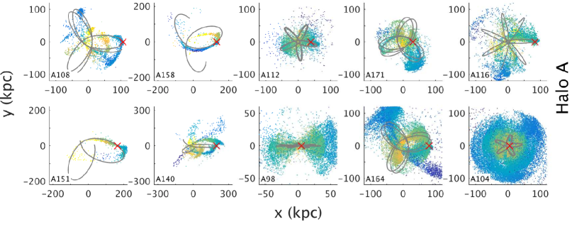
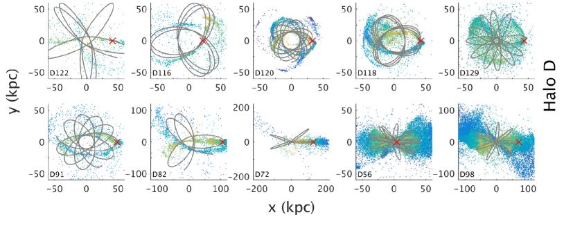
Figure 4: The same as Fig. 3 but now overplotting orbits integrated in the best fitting spherical potential to halo Aq-A (top panels) and halo Aq-D (bottom panels). The orientation of the streams has been changed such that the $z$-direction corresponds with the mean angular momentum of the particles. The plotted orbit is that of a particle (indicated with a red cross) near or in the bound part of the progenitor and has been evolved 4 Gyr forward and backwards in time assuming a static spherical potential.

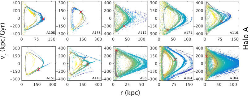
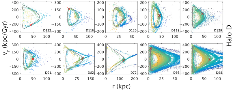
Figure 5: The same as Fig. 4 but now showing the $r$-$v_{r}$ projection for halo Aq-A (top panels) and halo Aq-D (bottom panels).

As a first step in our characterisation of streams, and for simplicity, we explore how orbits integrated in the best fitting spherical potential follow the trajectories delineated by the streams. For the relatively massive progenitors we naturally expect worse agreement, as discussed below. The initial conditions of the orbit were taken from a particle located in the highest density portion of the stream (typically a bound particle in the progenitor). We integrate this particle forward and backwards for 4 Gyr in our best fitting NFW potential to approximately match the streams’ length.

In Fig. 4 we show the resulting orbits on the streams, but in an orientation where the $z$-axis is in the direction of the mean angular momentum of the stream. An overview of the apocentre and pericentre distances of the spherical orbits is given in Appendix A. For thinner streams, with only one or two wraps, the orbits seem to follow the stream, such as for A158 and A151, but also the much thicker A164 has at least one loop reasonably matched. Many of the heavier streams that have more wraps show a big difference in radial extent when compared to the orbits, with stream A104 giving one of the least satisfactory results. This is not too surprising given that the spherical potential only supports a very limited range of orbit families. Also, a single orbit cannot fit the stream’s radial extent because this depends on the range of energies of the particles, and this is particularly large for some of our objects.

In Fig. 5 we show the streams in the $r$-$v_{r}$ plane with the corresponding orbits overlaid. For all objects individual stream wraps are discernible, even for those objects that are very massive and well phase-mixed. For these it is clear that the radial extent is not well matched by the orbits, as discussed earlier. Part of the complex structure seen in this phase-space projection may also be attributed to the triaxiality of the true potential. Nonetheless, in all cases the spherically integrated orbit seems to match reasonably at least a single wrap. Often the still bound part of the progenitor appears as a vertical diamond shaped object in the stream. Its location coincides quite well with the location of the highest density of the stream, which was chosen to define the initial conditions for the orbital integration and is indicated by the red cross. Near the progenitors of D82 and D72 we see very long arms that at the ends seem to dissolve in the stream. Most likely these particles are not yet completely unbound from the progenitor (see e.g. Gibbons et al. 2014)

We conclude that our orbits do reproduce some of the wraps of the streams, but typically they lack the complexity that is seen in the Aquarius simulations’ streams. This is partially because a single orbit cannot represent these streams stream well, but for a major part because the spherical potential does not support the exact same types of orbits.

3 Action-angle behaviour of Aquarius streams in
spherical potentials

3.1 General behaviour in a static potential

We now investigate the properties of our streams in action-angle space, where their behaviour is expected to be particularly simple. For an individual particle in a static potential, angles evolve linearly with time as

$$\theta_{i}(t)=\Omega_{i}t+\theta_{i}(0),$$ (2)

here $\Omega_{i}$ are the orbital frequencies, which only depend on the adiabatically invariant actions and hence are constant. For an ensemble this implies the spread in angles evolves as

$$\Delta\theta_{i}(t)=\Delta\Omega_{i}t+\Delta\theta_{i}(0).$$ (3)

For streams that have evolved long enough ($t\gg\Omega_{i}^{-1}$) we can ignore the initial angle spread $\Delta\theta_{i}(0)$, and therefore the appearance of the stream in angle and frequency is rather similar, with the stream in angle space being stretched out in time.

We can understand the shape in frequency space more quantitatively using a Taylor expansion of the orbital frequencies $\Omega_{i}$ with respect to the actions $J_{j}$ (Helmi & White 1999)

$$\Delta\Omega_{i}\approx H_{ij}\Delta J_{j},$$ (4)

with the spreads measured with respect to the centre of mass of the progenitor, and the Hessian of the Hamiltonian $H_{ij}$ also evaluated at this point. If we diagonalise the Hessian (and assuming the Einstein notation convention)

$$H_{ij}\Delta J_{j}=V_{ik}D_{kl}(V^{T})_{lj}\Delta J_{j}=V_{il}\left(\lambda_{l}\Delta\tilde{J}_{l}\right),$$ (5)

with $V$ the matrix of eigenvectors $\@vec{e}_{i}$ of $H_{ij}$ (as its columns), $D_{kl}$ the diagonal matrix with the eigenvalues $\lambda_{i}$, and $\Delta\tilde{J}_{l}=V_{lj}^{T}\Delta J_{j}$, the action spreads in the eigenspace. In vector notation this expression takes the simpler form

$$\@vec{\Delta\Omega}=\sum_{i}\lambda_{i}\,\Delta\tilde{J}_{i}\,\@vec{e}_{i}.$$ (6)

Generally one of the eigenvalues of the Hessian is much larger than the others , and this is responsible for the stream being a thin 1-D structure in frequency space(and therefore also in angle space), that is elongated mostly in the direction associated to the corresponding eigenvector (Tremaine 1999). Note here that also the relative magnitude of the action spreads is relevant for the direction in which the frequency distribution is elongated.

The action-angle coordinates of course depend on the underlying potential. For example, in a spherical potential there are two independent frequencies $\Omega_{\phi}$ and $\Omega_{r}$ (and $\Omega_{\phi}=\Omega_{\vartheta}$, apart from a possible sign difference), and therefore for sufficiently long times $\Delta\theta_{r}(t)=\Delta\Omega_{r}t$ and $\Delta\theta_{\phi}(t)=\Delta\Omega_{\phi}t$. This implies that in this regime in the space of angles, streams follow a straight line with slope $S(\Delta\theta)=\Delta\theta_{\phi}/\Delta\theta_{r}$ which is the same slope as in frequency space $S(\Delta\Omega)=\Delta\Omega_{\phi}/\Delta\Omega_{r}$.

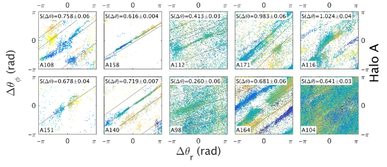
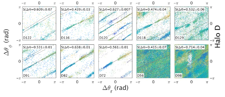
Figure 6: The $\theta_{r}$-$\theta_{\phi}$ space for the streams selected from halo Aq-A (top panels) and Aq-D (bottom panels) shown in previous figures. The angles have been computed using the best fitting spherical NFW potentials, and are centred around the most bound particle in the progenitor, or around a particle closest to the highest density in $\theta_{r}$-$\theta_{\phi}$ space. The colours indicate the energy gradient assuming the spherical NFW potential. The distributions were fitted with straight lines after removing generously particles still bound to the progenitor. The insets show the fitted slope and its error as estimated from bootstrapping 200 times.

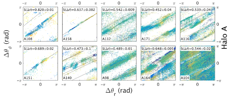
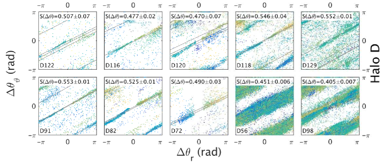
Figure 7: As Fig. 6, but now the $\theta_{r}$-$\theta_{\vartheta}$ angle space for the streams selected from halo Aq-A (top panels) and Aq-D (bottom panels).

3.2 Computing the angles and frequencies

In this section, and as a first approximation, we assume the mass distribution of the Aquarius halos is represented by our best fitting spherical NFW potential. For this potential we compute the actions, angles and frequencies (see Goldstein 1950; Binney & Tremaine 2008, for the general procedure). As noted above, in a spherical potential, $\Omega_{\phi}$ and $\Omega_{\vartheta}$ are equal by definition, however the corresponding angles $\theta_{\vartheta}$ and $\theta_{\phi}$ will be different for the particles in our streams. This is because they depend on the current positions and velocities of the particles which are the result of the evolution in a different potential than used to compute the angles.

In Figs. 6 and 7 we show the distribution of particles in the $\theta_{r}$-$\theta_{\phi}$ and $\theta_{r}$-$\theta_{\vartheta}$ spaces respectively. The most striking feature in these figures is that each of the streams is distributed along more or less straight lines (Sanders & Binney 2013a; Buist & Helmi 2015), even though the host potential is really not spherical. For all streams, the behaviour in $\theta_{r}$-$\theta_{\vartheta}$ space is generally cleaner and the individual streams are seen more clearly than in $\theta_{r}$-$\theta_{\phi}$ space. That such a difference exists is of course a reflection of the halos being non-spherical.

Table 1: Overview of the fitted slopes obtained assuming a spherical NFW potential for Aquarius haloes Aq-A and Aq-D from Figs. 6, 7, and 8.

Stream	$S(\Delta\theta_{r,\phi})$	$S(\Delta\theta_{r,\vartheta})$	$S(\Delta\Omega)$	Stream	$S(\Delta\theta_{r,\phi})$	$S(\Delta\theta_{r,\vartheta})$	$S(\Delta\Omega)$
A98	$0.260\pm 0.06$	$0.489\pm 0.01$	$0.566\pm 0.001$	D56	$0.415\pm 0.07$	$0.451\pm 0.006$	$0.561\pm 0.0004$
A104	$0.641\pm 0.03$	$0.544\pm 0.02$	$0.568\pm 0.0005$	D72	$0.561\pm 0.01$	$0.490\pm 0.03$	$0.585\pm 0.002$
A108	$0.758\pm 0.06$	$0.820\pm 0.01$	$0.525\pm 0.002$	D82	$0.638\pm 0.01$	$0.525\pm 0.01$	$0.544\pm 0.001$
A112	$0.413\pm 0.03$	$0.542\pm 0.009$	$0.577\pm 0.002$	D91	$0.531\pm 0.01$	$0.553\pm 0.01$	$0.571\pm 0.002$
A116	$1.024\pm 0.04$	$0.539\pm 0.04$	$0.574\pm 0.003$	D98	$0.714\pm 0.04$	$0.405\pm 0.007$	$0.548\pm 0.0003$
A140	$0.719\pm 0.007$	$0.473\pm 0.1$	$0.618\pm 0.002$	D116	$0.439\pm 0.03$	$0.477\pm 0.02$	$0.605\pm 0.002$
A151	$0.678\pm 0.04$	$0.689\pm 0.02$	$0.710\pm 0.005$	D118	$0.474\pm 0.04$	$0.546\pm 0.04$	$0.566\pm 0.002$
A158	$0.616\pm 0.004$	$0.637\pm 0.002$	$0.652\pm 0.003$	D120	$0.627\pm 0.007$	$0.470\pm 0.07$	$0.579\pm 0.001$
A164	$0.681\pm 0.06$	$0.648\pm 0.005$	$0.632\pm 0.0008$	D122	$0.609\pm 0.07$	$0.507\pm 0.07$	$0.588\pm 0.004$
A171	$0.983\pm 0.06$	$0.452\pm 0.04$	$0.572\pm 0.002$	D129	$0.532\pm 0.06$	$0.552\pm 0.01$	$0.575\pm 0.002$

We fit straight lines to the streams, in analogy to what we did in Buist & Helmi (2015), and the results are given also in the figures and in Table 1. Our method to fit lines to the distributions of streams in angle space is discussed in Appendix D. We fit the distributions in $\theta_{r}$-$\theta_{\phi}$ and $\theta_{r}$-$\theta_{\vartheta}$ separately because as we just saw, the behaviour in these spaces is different. Particles that are still bound to the progenitor are removed from the fitting procedure because they are not expected to follow the general action-angle behaviour of the stream. The result of this removal is clearly visible for example in stream D72 and A164 where we see a gap in the middle of the distribution in angle space.

The fitting procedure puts into evidence several noticeable distortions in angle space because the different wraps of a stream are not always on parallel lines, such as for stream A108 and A116. Much more subtle is the deviation seen in the bottom-left of stream A158. These distortions clearly pose a challenge to the determination of the slope. For this reason we have to take the slopes determined with our method generally with some care (especially in the case of A116) as the quoted errors do not account for such systematic uncertainties. A quick visual inspection usually helps to evaluate the outcome and the reliability of the fit. The slopes in $\theta_{r}$-$\theta_{\phi}$ space are much more varied than those in $\theta_{r}$-$\theta_{\vartheta}$ space, which especially for halo Aq-D all cluster around $0.5$. Generally, we also notice that the streams in halo Aq-D seem less distorted than those in halo Aq-A.

In our selection of streams we also included several objects on very radial orbits, and whose debris is distributed in an hour-glass shape in configuration space, such as A98, D56 and D98. In $\theta_{r}$-$\theta_{\phi}$ space they seem very mixed and do not show very distinct structures, yet their behaviour in $\theta_{r}$-$\theta_{\phi}$ is remarkable with streams along straight lines being clearly apparent (see e.g. D56 and D98 in Fig. 7). These objects are typically more massive and have deposited debris close to the centre of the halo and therefore are more phase mixed.

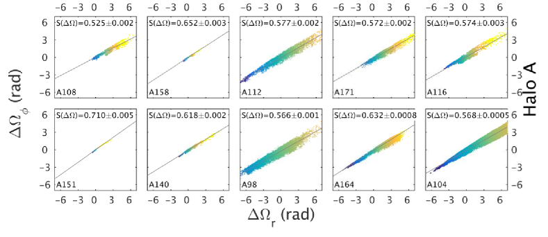
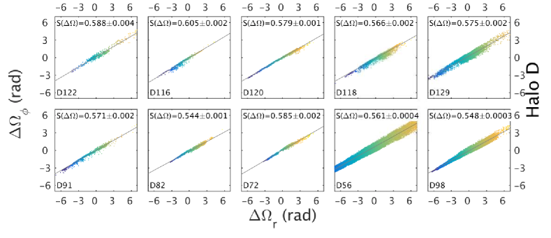
Figure 8: Frequency distributions computed using the best fitting spherical potentials for our selection of streams from halo Aq-A (top panels) and Aq-D (bottom panels) shown in previous figures. The panels are centred around the same particle as in Figs. 6 and 7. The distributions were fitted with straight lines after removing generously the bound particles from the progenitor. The colours indicate the energy gradient for the spherical potential. The insets show the fitted slope and estimated errors.

3.3 Comparing the slopes in frequency and angle space

In Fig. 8 we show the frequency distributions of the streams. These follow closely a straight line, although sometimes they are quite thick. For A108 and A116 the width in frequency space is not everywhere the same. This is one of the signatures expected when using the wrong potential to compute the frequencies. The determination of the fitted slopes is more robust in frequency space, and these show a considerably smaller range than the slopes in angle space.

The slopes in angle space and frequency space differ, especially when comparing to the $\theta_{r}$-$\theta_{\phi}$ space to frequency space. They are expected to be equal in the true (static) potential (Sanders & Binney 2013a, b). In Buist & Helmi (2015) we found that in a time-dependent potential, the slope in angle space is steeper than in frequency space (i.e. $S(\Delta\theta)>S(\Delta\Omega)$). Therefore, since the potentials in the Aquarius N-body simulations have grown in time we might expect the angle space slope to be larger. For some of the streams in our sample this is indeed the case, but there are quite a few streams for which this does not hold, such as D116 and A112, for which the magnitude of the angle-frequency difference is far greater than what can be expected from (adiabatic) evolution of the halo. Also in $\theta_{r}$-$\theta_{\vartheta}$ space many streams are not in line with our expectations. Overall we find that in $\theta_{r}$-$\theta_{\vartheta}$, 28 of the 35 streams have a larger slope in frequency than in angle space, i.e. they do not follow the expected behaviour, and while for $\theta_{r}$-$\theta_{\phi}$, this is the case for 17 out of the 35 streams.

The simulations of Buist & Helmi (2015) that follow the evolution of streams in a spherical potential, show that differences between the slopes can be obtained when the wrong potential is assumed. For example, $S(\Delta\theta)-S(\Delta\Omega)>0$ when the enclosed mass is too high, and $S(\Delta\theta)-S(\Delta\Omega)<0$ when the enclosed mass is too low. We therefore may attribute the differences in slope to having assumed an incorrect potential (mostly in shape), and not to time-dependence.

3.4 Influence of the potential

We also expect an energy gradient to be present along a stream (Buist & Helmi 2015), and although this is visible in frequency space it is less clear in angle space. This is not unexpected as the frequencies depend on energy (via the actions) and more energetic particles move faster, while, on the other hand, the angles depend also on other phase-space coordinates. Even small (of order $10$%) differences in the characteristic parameters of the potential can lead to the energy gradient being lost in angle space, even when the stream itself has a normal appearance (Buist & Helmi 2015). An exception is A164 in $\theta_{r}$-$\theta_{\phi}$-space, which does seem to have a continuous energy gradient when following the stream along its various wraps.

To see if the behaviour in angle space and the energy gradient could be improved we experimented by changing one of the characteristic parameters, namely the enclosed mass for the particular case of A158. However we were unable to remove the bend seen at the bottom-left in $\theta_{r}$-$\theta_{\phi}$ space, a behaviour that in the spherical case is known to be indicative of wrong values of the characteristic parameters of the potential. It seems clear from the analysis presented in this section that it is the shape of the potential that is wrong rather than the value of the enclosed mass.

We conclude that streams can still look rather regular in angle and frequency space when making an incorrect assumption about the shape of the potential, even if they evolved in a potential that grew via accretion and merging. In later sections of this Paper we will investigate the conditions for streams to be distributed along straight lines such as those seen in Figs. 6, 7, and 8.

4 Test-particle simulations of streams in axisymmetric potentials

The Aquarius halos are not spherically symmetric, and it is important to understand which of the deviations seen in the streams’ behaviour in angle space arise from having assumed a spherical potential. Rather than attempting to study their dynamics in a full triaxial potential, we add only one degree of complexity and now analyse a set of example streams evolved in the axisymmetric Kuzmin-Kutuzov Staeckel potential (Dejonghe & de Zeeuw 1988) with similar density axis ratios as halo Aq-D of the Aquarius simulations.. For the streams we have used as initial orbital conditions those extracted from the present-day positions and velocities of particles in halo Aq-D (as described in Sec. 2.4). An axisymmetric Staeckel potential allows for a relatively straightforward computation of the actions and angles. This implies that we can directly compare their behaviour using true action-angles to those computed assuming a spherical approximation to this potential.

4.1 Potential set-up

To motivate our choice of the characteristic parameters of our axisymmetric potential, we use the Aquarius halos. These halos are triaxial, and may be described with two axis ratios: $q=c/a$ (long to short axis ratio) and $s=b/a$ (intermediate to long axis ratio, i.e. $a\geq b\geq c$). A useful quantity is the triaxiality parameter (Franx et al. 1991)

$$T=\frac{a^{2}-b^{2}}{a^{2}-c^{2}}=\frac{1-s^{2}}{1-q^{2}},$$ (7)

which is zero for an oblate halo and equals unity for a prolate halo. Halos Aq-A and Aq-D have triaxiality parameters between $T=2/3$ and $1$ at a radius of $50$ kpc, making them somewhat more prolate, with halo Aq-A being more triaxial than halo Aq-D. Therefore these halos are not in the range of being extremely triaxial ($T=1/3$ to $2/3$, see also Warren et al. 1992), although at larger radii their triaxiality increases (Vera-Ciro et al. 2011).

The functional form of the Kuzmin-Kutuzov potential is given by (Dejonghe & de Zeeuw 1988):

$$\Phi_{\textrm{K}}(R,z)=-\frac{GM_{\textrm{K}}}{\sqrt{a_{\textrm{K}}^{2}+c_{\textrm{K}}^{2}+R^{2}+z^{2}+2\sqrt{a_{\textrm{K}}^{2}c_{\textrm{K}}^{2}+R^{2}c_{\textrm{K}}^{2}+a_{\textrm{K}}^{2}z^{2}}}},$$ (8)

where $M_{\rm K},a_{\rm K},c_{\rm K}$ are characteristic mass and scale parameters, respectively. A coordinate transformation to prolate ellipsoidal coordinates ($\lambda$, $\nu$, $\phi$) leads to a simple expression

$$\Phi_{\textrm{K}}(\lambda,\nu)=-\frac{GM_{\textrm{K}}}{\sqrt{\lambda}+\sqrt{\nu}},$$ (9)

where the relations between $\lambda$, $\nu$ and $R$, $z$ can be expressed as

$$\begin{split}\lambda\nu=c_{\textrm{K}}^{2}R^{2}+a_{\textrm{K}}^{2}z^{2}+a_{\textrm{K}}^{2}c_{\textrm{K}}^{2},\\ \lambda+\nu=R^{2}+z^{2}+a_{\textrm{K}}^{2}+c_{\textrm{K}}^{2}.\end{split}$$ (10)

We take $\lambda>\nu$. Depending on the ratio $c_{\textrm{K}}/a_{\textrm{K}}$, this coordinate system can be used to represent a prolate ($q_{\textrm{K}}>1$) or an oblate ($q_{\textrm{K}}<1$) mass distribution (see also the discussion in Dejonghe & de Zeeuw 1988). The potential in Eq. (9) reduces in the spherical limit ($a_{\textrm{K}}=c_{\textrm{K}}$) to Henon’s isochrone potential (Dejonghe & de Zeeuw 1988; Henon 1959). For convenience we link the parameters $M_{\textrm{K}}$, $a_{\textrm{K}}$ and $c_{\textrm{K}}$ to the isochrone scale radius $r_{\textrm{iso}}$ and scale mass $M_{\textrm{iso}}$, and introduce the flattening parameter $q_{\textrm{K}}\equiv c_{\textrm{K}}/a_{\textrm{K}}$. We define the isochrone scale mass as $M_{\textrm{iso}}=M_{\textrm{isochrone}}(r_{\textrm{iso}})$, such that

$$\begin{split}M_{\textrm{K}}&=M_{\textrm{iso}}\left(\frac{3}{\sqrt{2}}-2\right)^{-1},\\ a_{\textrm{K}}&=r_{\textrm{iso}}\frac{2}{1+q_{\textrm{K}}},\\ c_{\textrm{K}}&=r_{\textrm{iso}}\frac{2q_{\textrm{K}}}{1+q_{\textrm{K}}}.\end{split}$$ (11)

These relations satisfy $a_{\textrm{K}}+c_{\textrm{K}}=2r_{\textrm{iso}}$, i.e. the isochrone scale radius is the average of the Kuzmin-Kutuzov axis lengths. For the determination of the numerical values of the parameters we refer to Appendix C, where we set $q_{\textrm{K}}=1.87$, $M_{\textrm{iso}}=1.58\times 10^{11}$ M_⊙ and $r_{\textrm{iso}}=22.84$ kpc.

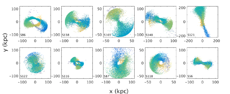
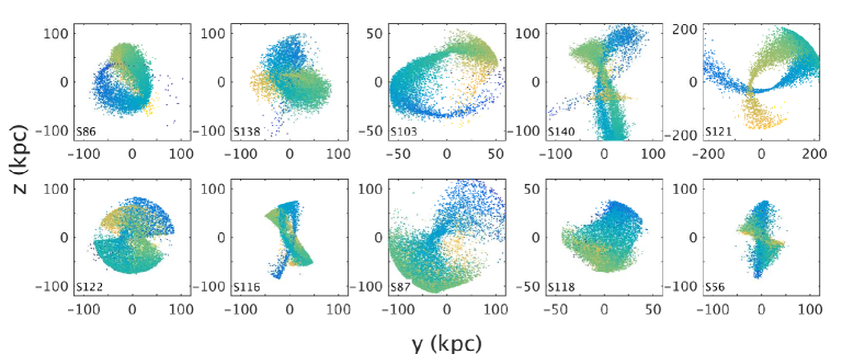
Figure 9: Spatial distribution of our selection of test-particle streams after 10 Gyr of evolution in the axisymmetric Kuzmin-Kutuzov potential. The colours represent the energy gradient with the most bound particles in yellow and those least bound in blue. The $z$-axis is aligned with the major axis of the potential.

4.2 Streams set-up

As mentioned earlier we use a subset of the streams’ positions and velocities extracted from the Aquarius simulations to evolve our test-particle simulations. The stream progenitor is composed of 10,000 particles that follow an isotropic Gaussian distribution in position and velocity, characterised by dispersions $\sigma_{\textrm{pos}}=0.3$ kpc and $\sigma_{\textrm{vel}}=10$ kpc/Gyr respectively. This can be roughly translated into a progenitor mass $M$ using that $\sigma_{\textrm{vel}}^{2}\sim GM/R$ and where we take $R=\sigma_{\textrm{pos}}$, which results in $M\approx 7.4\times 10^{7}$ M_⊙. The orbits are integrated for $10$ Gyr in the Kuzmin-Kutuzov potential with the parameters derived from Aquarius halo D.

Fig. 9 shows our streams, where the inset labels are the IDs of the corresponding Aq-D streams (e.g. S140 is based on the position and velocity of one particle in D140). Recall that it is not our goal to reproduce the original streams from the Aquarius halos in the axisymmetric limit, but to understand the behaviour of streams in the non-spherical regime.

4.3 Action-angles in the true potential

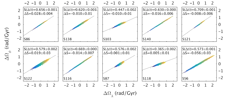
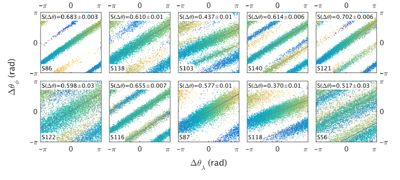
Figure 10: Test-particle streams in the true $\lambda$ - $\phi$ frequency (top) and angle (bottom) spaces after 10 Gyr of evolution in the Kuzmin-Kutuzov potential. The colours represent the energy gradient with the most bound particles in yellow and those least bound in blue. The panels have been centred on the current position of the centre of mass of the progenitor system. The insets give the best-fitting slopes to the distributions as well as the angle-frequency misalignment $\Delta S$.

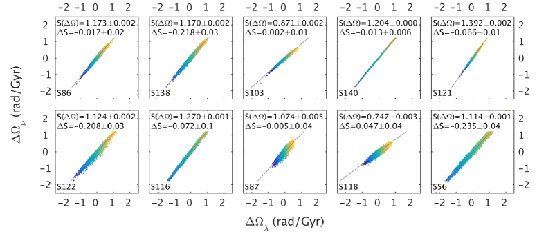
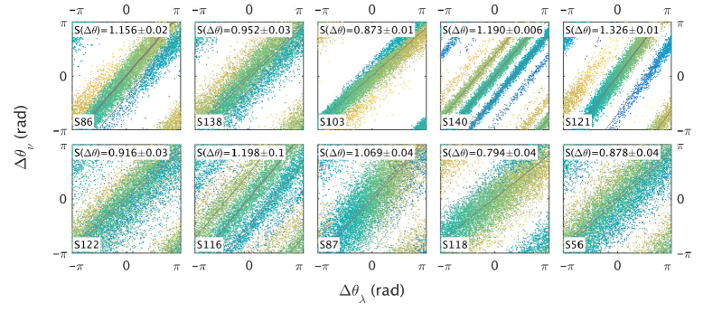
Figure 11: Same as in Fig. 10, but now for the $\nu$ - $\phi$ frequency and angle spaces.

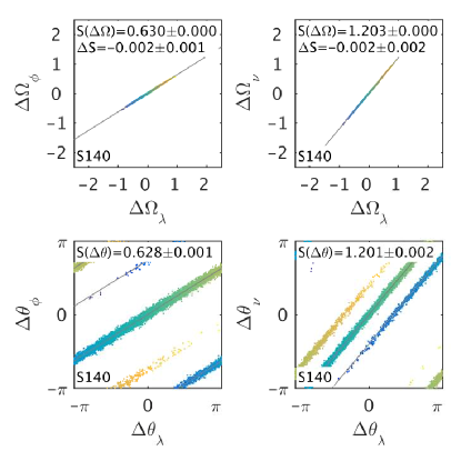
Figure 12: Stream S140 but now with a Carina-like progenitor, after 10 Gyr of evolution in the Kuzmin-Kutuzov potential. The colours and insets are the same as in Fig. 10. With the smaller progenitor the stream is much thinner and the error on the fitting is significantly reduced, which basically removes the angle-frequency misalignment.

Table 2: Overview of the fitted slopes in Figs. 10 and 11 of our test-particle streams integrated in an axisymmetric Staeckel potential.

Stream	$S(\Delta\theta_{\lambda,\phi})$	$S(\Omega_{\lambda,\phi})$	$\Delta S_{\lambda,\,\phi}$	$S(\Delta\theta_{\lambda,\nu})$	$S(\Omega_{\lambda,\nu})$	$\Delta S_{\lambda,\,\nu}$
S56	$0.517\pm 0.03$	$0.573\pm 0.0006$	$-0.056\pm 0.03$	$0.878\pm 0.04$	$1.114\pm 0.001$	$-0.235\pm 0.04$
S86	$0.683\pm 0.003$	$0.656\pm 0.0006$	$0.028\pm 0.004$	$1.156\pm 0.02$	$1.173\pm 0.002$	$-0.017\pm 0.02$
S87	$0.577\pm 0.01$	$0.576\pm 0.002$	$0.001\pm 0.01$	$1.069\pm 0.04$	$1.074\pm 0.005$	$-0.005\pm 0.04$
S103	$0.437\pm 0.01$	$0.447\pm 0.002$	$-0.010\pm 0.01$	$0.873\pm 0.01$	$0.871\pm 0.002$	$0.002\pm 0.01$
S116	$0.655\pm 0.007$	$0.669\pm 0.0005$	$-0.014\pm 0.007$	$1.198\pm 0.1$	$1.270\pm 0.001$	$-0.072\pm 0.1$
S118	$0.370\pm 0.01$	$0.365\pm 0.002$	$0.005\pm 0.01$	$0.794\pm 0.04$	$0.747\pm 0.003$	$0.047\pm 0.04$
S121	$0.702\pm 0.006$	$0.709\pm 0.0009$	$-0.008\pm 0.006$	$1.326\pm 0.01$	$1.392\pm 0.002$	$-0.066\pm 0.01$
S122	$0.598\pm 0.03$	$0.579\pm 0.002$	$0.019\pm 0.03$	$0.916\pm 0.03$	$1.124\pm 0.002$	$-0.208\pm 0.03$
S138	$0.610\pm 0.01$	$0.620\pm 0.001$	$-0.010\pm 0.01$	$0.952\pm 0.03$	$1.170\pm 0.002$	$-0.218\pm 0.03$
S140	$0.614\pm 0.006$	$0.630\pm 0.0004$	$-0.016\pm 0.006$	$1.190\pm 0.006$	$1.204\pm 0.0004$	$-0.013\pm 0.006$

For the Kuzmin-Kutuzov potential the Hamilton-Jacobi equation separates in prolate spheroidal coordinates ($\lambda$, $\nu$, $\phi$). This means that we can compute the true actions ($J_{\lambda}$, $J_{\nu}$, $J_{\phi}$), the corresponding frequencies, and the angles in a straightforward manner. At large distances from the centre $\lambda$ behaves like the radial coordinate $r$ from the spherical case, while $\nu$ follows almost the longitudinal angle $\vartheta$. For this reason, we will generally compare $\Omega_{\lambda}$ with $\Omega_{r}$, and $\Omega_{\nu}$ with $\Omega_{\vartheta}$ (and the same for their corresponding angles).

The results for each of the streams in Fig. 9 are shown in Fig. 10 and Fig. 11 for both projections of frequency space (top) and angle space (bottom). In angle space, the streams are distributed along straight lines (just as in frequency space), spreading out after 10 Gyr of evolution. The insets in the figures show the slopes obtained from fitting straight lines to the distributions, where the error is estimated from bootstrapping the fits 200 times. These results are also summarised in Table 2.

We also give in the top panels the angle-frequency misalignment $\Delta S=S(\Delta\theta)-S(\Delta\Omega)$, with the corresponding error. Notice that typically $|\Delta S|\sim 0.01-0.02$, which is larger than found by Buist & Helmi (2015) for the streams evolved in a static spherical potential. This is mostly due to the larger progenitor used here which causes the streams to be wider, and this has an impact both on the initial spreads and on the fitting procedure. This is explicitly demonstrated in Fig. 12, where we show a stream on the same orbit as S140 but now for the Carina-like progenitor ($\sigma_{\textrm{pos}}=0.1$ kpc and $\sigma_{\textrm{vel}}=5$ kpc/Gyr) used in Buist & Helmi (2015) and evolved for 10 Gyr. We see that the angle-frequency misalignment is now consistent with being zero.

5 Action-angle behaviour of streams in approximate potentials of varying shape

Thus far we have discussed mostly from a theoretical point of view what to expect in angle and frequency space in the true potential, and why streams are on straight lines. In this section we explore what happens when the wrong potential is used to compute the angles and frequencies. To this end we employ the test-particle simulations of Sec. 4 run in the axisymmetric Staeckel potential, but we will assume a spherical potential (Sec. 5.1), a Staeckel potential but with a different flattening parameter ($q_{\textrm{K}}^{\prime}=1/q_{\textrm{K}}$, Sec. 5.2), and a spherical potential with a more dissimilar radial mass distribution (Sec. 5.3). We also explore the effect of self-gravity in Sec. 5.4

5.1 Spherical approximation

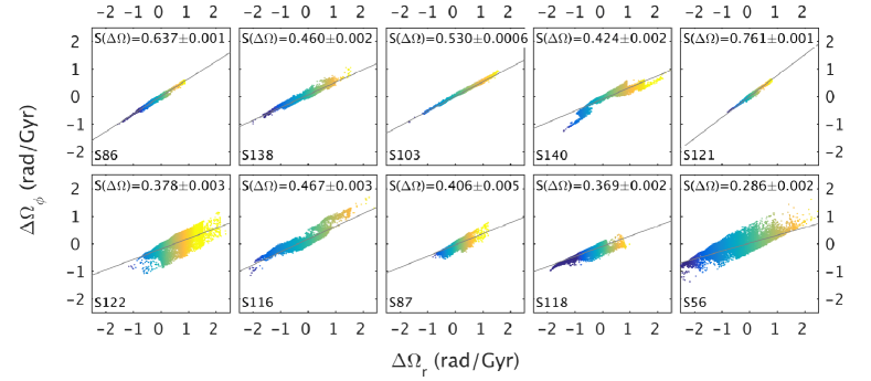
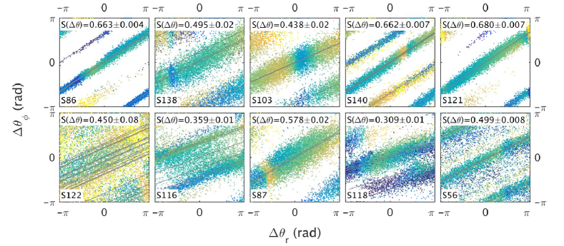
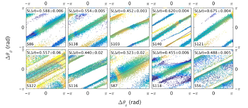
Figure 13: Test-particle streams evolved in the axisymmetric Kuzmin-Kutuzov potential and shown in Figs. 9-11, depicted now assuming a spherical approximation to the potential in the space of frequencies $\Delta\Omega_{r}$-$\Delta\Omega_{\phi}$ (top panels) and angles $\Delta\theta_{r}$-$\Delta\theta_{\phi}$ (middle panels) and $\Delta\theta_{r}$-$\Delta\theta_{\vartheta}$ (bottom panels). The colours represent the energy gradient in the isochrone potential. The panels have been centred on the progenitor position. The insets indicate the fitted slopes for the approximate potential. The errors were found by bootstrapping the fit 200 times.

We now compute the angles and frequencies for the test-particle simulations assuming the isochrone potential. This potential constitutes the spherical limit of the Kuzmin-Kutuzov potential, and its characteristic parameters were defined in Sec. 4.1. The resulting angle and frequency distributions are shown in Fig. 13, where we do not include the $\Omega_{r}$-$\Omega_{\vartheta}$ space as it is redundant in the spherical case. Instead, the behaviour in the angles $\theta_{\phi}$ and $\theta_{\vartheta}$ is relevant since these additionally depend on the physical location of the particles (which encodes information about the potential in which they were evolved as discussed earlier in Sec. 3). The characteristic parameters of the fitted straight lines are also listed in Table 3.

Table 3: Overview of the fitted slopes in Fig. 13 obtained assuming a spherical isochrone potential for our test-particle streams evolved in an axisymmetric Staeckel potential.

Stream	$S(\Delta\theta_{r,\phi})$	$S(\Delta\theta_{r,\vartheta})$	$S(\Delta\Omega)$
S56	$0.499\pm 0.008$	$0.488\pm 0.005$	$0.286\pm 0.002$
S86	$0.663\pm 0.004$	$0.588\pm 0.006$	$0.637\pm 0.001$
S87	$0.578\pm 0.02$	$0.523\pm 0.02$	$0.406\pm 0.005$
S103	$0.438\pm 0.02$	$0.452\pm 0.003$	$0.530\pm 0.0006$
S116	$0.359\pm 0.01$	$0.440\pm 0.02$	$0.467\pm 0.003$
S118	$0.309\pm 0.01$	$0.455\pm 0.006$	$0.369\pm 0.002$
S121	$0.680\pm 0.007$	$0.675\pm 0.004$	$0.761\pm 0.001$
S122	$0.450\pm 0.08$	$0.557\pm 0.06$	$0.378\pm 0.003$
S138	$0.495\pm 0.02$	$0.554\pm 0.005$	$0.460\pm 0.002$
S140	$0.662\pm 0.007$	$0.620\pm 0.004$	$0.424\pm 0.002$

In the top panel of Fig. 13 we show the resulting frequency distributions. We find that quite a few streams have become thicker and distorted in the spherical approximation to the potential in comparison to their behaviour in the true axisymmetric potential. Some of the streams seem quite irregular such as S140, a characteristic that was also seen for some of the Aquarius streams (see e.g. stream A107 in Fig. 8). As a consequence of the distortions, it is generally more difficult to fit straight lines to the frequency distribution, and therefore also the determination of their slopes is less reliable (see e.g. S122 and S138).

To understand this behaviour it is interesting to explore how orbits map onto frequency space if the frequencies are computed at each time step in the approximate spherical potential. This is show in Fig. 14 for two different orbits. The trajectories oscillate in frequency, while if the potential had been truly spherical they would collapse into a single point. These oscillations are therefore directly related to how well the isochrone potential represents the mass distribution. We take from this that the thickening of streams is caused by the degree to which the orbits of those particles are described by a spherical potential.

The central panel of Fig. 13 shows the $\theta_{r}$-$\theta_{\phi}$ space. Streams such as S103 and S121 appear quite similar to their counterparts in Fig. 10, plotted in their natural (true) angle space ($\theta_{\lambda}$-$\theta_{\phi}$). Notice that when the straight line fits look reasonable, the slopes in this spherical angle space and in the corresponding Staeckel angles are similar, differing by $\sim 0.05$. Like for the Aquarius streams, the slopes in $\theta_{r}$-$\theta_{\phi}$ span a range between $\sim 0.4-0.7$. In all cases, the streams have become thicker. The energy gradient along the streams seems especially discontinuous at some locations, while for some streams such as S140 and S121 it is somewhat better retained.

The bottom panels of Fig. 13 shows the angles $\theta_{r}$-$\theta_{\vartheta}$. The comparison of $\theta_{\lambda}$-$\theta_{\nu}$ to $\theta_{r}$-$\theta_{\vartheta}$ is less straightforward because $\Omega_{\vartheta}$ and $\Omega_{\nu}$ differ by a factor 2 in the spherical limit.

We conclude that using a spherical approximation to the potential leads to an increase of the spread in frequency space, by making the streams longer, wider and/or distorted, but the energy gradient remains quite intact in this space. The streams in angle space often look much more well-behaved, although they do become thicker and the energy gradient is not preserved. This good behaviour probably reflects that the spherical potential has the right average enclosed mass (as argued by Buist & Helmi 2015). We find that the fitted slopes in angle and frequency space deviate significantly from each other, indicating that the true potential in which the streams have evolved has not been used for the angle and frequency computations. We have explored possible correlations between slopes differences and orbital characteristics in our stream sample that could perhaps be used to infer the asphericity of the true potential. However, we found no specific trends in the differences in slopes between the angle and frequency spaces, nor between the angles in the spaces $\theta_{\theta}-\theta_{r}$) and $\theta_{\phi}-\theta_{r}$).

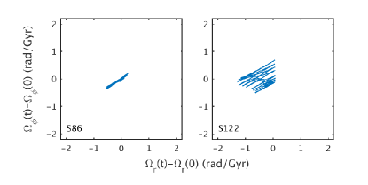
Figure 14: Frequencies computed in the limiting spherical potential for two progenitor orbits from the test-particle simulations in the Kuzmin-Kutuzov potential (see Fig. 9).

5.2 Axisymmetric Staeckel potential with different flattening

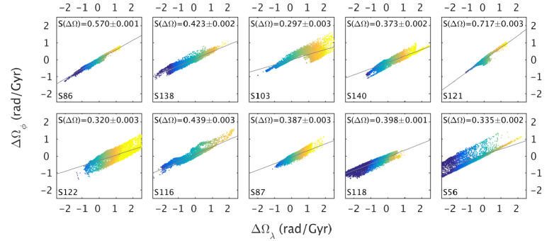
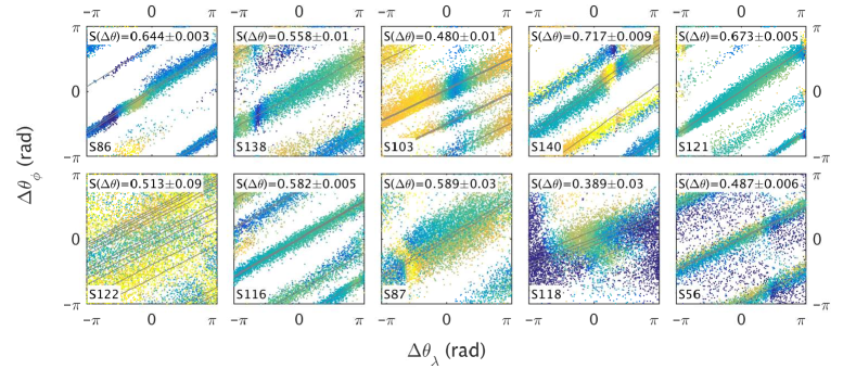
Figure 15: Test-particle streams from Fig. 9- 11 with the frequencies and angles in the $\lambda$-$\phi$ projections computed for a Staeckel potential with flattening $q_{\textrm{K}}^{\prime}=1/q_{\textrm{K}}$. The colours represent the energy gradient with the most bound particles in yellow and the least bound particles in blue.

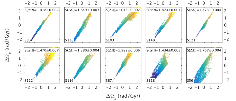
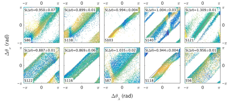
Figure 16: Same as Fig. 15 but now showing the $\lambda$-$\nu$ projections.

Table 4: Overview of the fitted slopes in Figs. 15 and 16 obtained for our test-particle streams assuming an axisymmetric Staeckel potential with flattening $q_{\textrm{K}}^{\prime}=1/q_{\textrm{K}}$.

Stream	$S(\Delta\theta_{\lambda,\phi})$	$S(\Delta\Omega_{\lambda,\phi})$	$S(\Delta\theta_{\lambda,\nu})$	$S(\Delta\Omega_{\lambda,\nu})$
S56	$0.487\pm 0.006$	$0.335\pm 0.002$	$0.956\pm 0.01$	$1.767\pm 0.004$
S86	$0.644\pm 0.003$	$0.570\pm 0.001$	$0.950\pm 0.07$	$1.418\pm 0.002$
S87	$0.589\pm 0.03$	$0.387\pm 0.003$	$1.035\pm 0.02$	$1.582\pm 0.006$
S103	$0.480\pm 0.01$	$0.297\pm 0.003$	$0.994\pm 0.004$	$1.043\pm 0.002$
S116	$0.582\pm 0.005$	$0.439\pm 0.003$	$0.869\pm 0.06$	$1.380\pm 0.004$
S118	$0.389\pm 0.03$	$0.398\pm 0.001$	$0.944\pm 0.004$	$1.434\pm 0.005$
S121	$0.673\pm 0.005$	$0.717\pm 0.003$	$1.309\pm 0.01$	$1.473\pm 0.004$
S122	$0.513\pm 0.09$	$0.320\pm 0.003$	$0.887\pm 0.01$	$1.470\pm 0.007$
S138	$0.558\pm 0.01$	$0.423\pm 0.002$	$0.899\pm 0.01$	$1.649\pm 0.003$
S140	$0.717\pm 0.009$	$0.373\pm 0.002$	$1.004\pm 0.03$	$1.474\pm 0.004$

In this section we compute the angles and frequencies for the Kuzmin-Kutuzov potential, but now assuming a flattening $q_{\textrm{K}}^{\prime}=1/q_{\textrm{K}}$, which reverses the axis lengths $a_{\textrm{K}}$ and $c_{\textrm{K}}$ compared to the true potential. For the simulations of Sec. 4 we used a prolate potential, and inverting $q_{\textrm{K}}$ results in an oblate shape.

The resulting distributions in frequency and angle space are shown in Figs. 15, 16, and listed in Table 4, and qualitatively are very similar to what we saw in Sec. 5.1 and in previous figures. The frequency distributions are even more broadened than when assuming a spherical potential, and for some of the streams such as S56 also more extended (i.e. beyond the boundaries of the box, which we retained for easier comparison, and which is centred on the progenitor’s centre of mass). This broadening appears to be asymmetric with respect to the progenitor. As in the previous section, the energy gradient in frequency space remains almost intact while in angle space it almost cannot be discerned.

The slopes fitted to the angle and frequency distributions differ considerably, which we, for a large part can attribute to the difficulty of the fitting in frequency space. In both angle spaces we see that some of the streams depict small scale wiggles, such as streams S86, S118 and S140, which are more apparent in $\theta_{\lambda}$-$\theta_{\nu}$ space. This is probably because the shape of the potential is significantly different from the true form, and from the spherical shape assumed in the previous section.

5.3 Spherical approximation with incorrect radial form

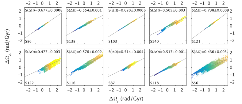
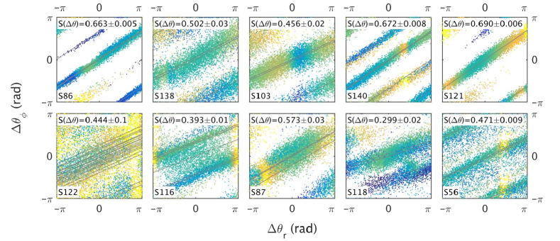
Figure 17: Test-particle streams from Fig. 9–11 with the frequencies $\Delta\Omega_{r}$-$\Delta\Omega_{\phi}$ (top panels) and angles $\Delta\theta_{r}$-$\Delta\theta_{\phi}$ (middle panels) and $\Delta\theta_{r}$-$\Delta\theta_{\vartheta}$ (bottom panels), computed using an NFW potential that has the same slope at a fixed radius as the limiting spherical isochrone potential (see Fig. 21). The colours represent the energy gradient in the NFW potential. The panels have been centred on the progenitor position. The insets indicate the fitted slopes for the approximate potential. The errors were found by bootstrapping the fit 200 times.

Table 5: Overview of the fitted slopes in Fig. 17 obtained assuming a spherical NFW potential for our test-particle streams evolved in an axisymmetric Staeckel potential.

Stream	$S(\Delta\theta_{r,\phi})$	$S(\Delta\theta_{r,\vartheta})$	$S(\Delta\Omega)$
S56	$0.471\pm 0.009$	$0.470\pm 0.005$	$0.436\pm 0.003$
S86	$0.663\pm 0.005$	$0.593\pm 0.006$	$0.677\pm 0.0008$
S87	$0.573\pm 0.03$	$0.544\pm 0.02$	$0.514\pm 0.004$
S103	$0.456\pm 0.02$	$0.456\pm 0.003$	$0.620\pm 0.0006$
S116	$0.393\pm 0.01$	$0.462\pm 0.02$	$0.576\pm 0.002$
S118	$0.299\pm 0.02$	$0.484\pm 0.009$	$0.517\pm 0.001$
S121	$0.690\pm 0.006$	$0.682\pm 0.006$	$0.738\pm 0.0009$
S122	$0.444\pm 0.1$	$0.609\pm 0.08$	$0.477\pm 0.003$
S138	$0.502\pm 0.03$	$0.538\pm 0.005$	$0.554\pm 0.001$
S140	$0.672\pm 0.008$	$0.614\pm 0.006$	$0.505\pm 0.003$

We now focus on the impact of computing the actions and angles in a spherical potential whose radial dependence is quite different from the Kuzmin-Kutuzov potential in the spherical limit. We explore an NFW potential that has the same enclosed mass and mass slope at $r_{\textrm{fix}}=50$ kpc (see also Fig. 21).

In Fig. 17 and Table 5 we show the resulting distribution of these angles and frequencies for the streams evolved in the axisymmetric Kuzmin-Kutuzov potential of Sec. 4. At first sight, many of the streams look very similar to those in Fig. 13, which corresponds to the computations assuming a spherical isochrone mass distribution.

In frequency space we see that some of the streams are longer and thinner (see e.g. S140 and S118). The slopes derived from fitting straight lines to these distributions are different from those computed in the isochrone potential, such as for S86 and S103. In angle space the differences are more subtle, and the typical difference between the fitted slopes between the isochrone and NFW cases is $\sim 0.05$, which is comparable to the estimated error in the fit, but also the incorrect shape of the potential may contribute here. The energy gradient in angle space for the isochrone and NFW potentials is not always the same, with the isochrone potential showing more fluctuations in the $\theta_{r}$ direction. Overall we find that the frequencies are the most sensitive to the potential, but the differences are small because the slope and the enclosed mass at $r_{\textrm{fix}}=50$ kpc are equal for the NFW and isochrone profiles. The behaviour in frequency and angle space is only slightly worse than for the spherical isochrone potential.

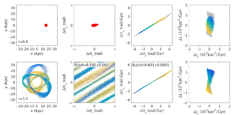
Figure 18: Projections of configuration, angle, frequency and action space at $t=0$ (top panels) and $t=3.5$ Gyr (bottom panels) for an N-body stream evolved in a spherical NFW potential. The first column shows the projection of the stream on the orbital plane of the progenitor. Particles still bound to the progenitor are plotted in red. In the third column we have overlaid the distribution of frequencies at $t=10$ Gyr in grey. In the panels on the right we also show the final distribution of actions at $t=10$ Gyr in grey. The actions, angles and frequencies have been centred on the coordinates of the centre of mass of the progenitor and the colours represent the energy gradient.

5.4 The effects of self-gravity

In reality the progenitors of streams will initially be bound by their own self-gravity. Particles that become unbound with time will typically be released at specific points along the orbit (close to pericentre), rather than continuously as modelled thus far. This results in the leading and trailing arms being offset from each other in configuration space (Johnston 1998) and in energy-angular momentum space (Gibbons et al. 2014). The process of disruption also causes particles to define a bow-tie structure in action (and energy-angular momentum) space. Since one of our goals is to understand the properties of streams in the cosmological Aquarius N-body simulations, we attempt here to establish what the effect of self-gravity is on the distribution of particles in frequency and angle spaces.

To this end, we simulated the evolution of a $3.7\times 10^{8}$ $\textrm{M}_{\odot}$ progenitor for 10 Gyr on an orbit with $r_{\textrm{apo}}=23.6$ kpc and $r_{\textrm{peri}}=10.2$ kpc in a spherical NFW potential with $M_{\textrm{s}}=1.5\times 10^{11}$ $\textrm{M}_{\odot}$ and $r_{\textrm{s}}=12$ kpc using an N-body code that uses a quadrupole expansion to model the internal gravitational potential of the system (Helmi & White 2001). Fig. 18 shows snapshots for $t=0$ and $t=3.5$ Gyr. The left panels plot the projection of the stream on the progenitor’s orbital plane, where the red particles correspond to those that are (still) bound. The stream has already spread out significantly by $t=3.5$ Gyr because the progenitor is large and the orbit is rather confined to the inner regions of the host, which results in fast evolution. By this time, the progenitor has almost completely dissolved (i.e. only a few particles are marked in red).

In the second panel we show the angle distribution initially and at $3.5$ Gyr, with the particles bound to the progenitor marked in red. By $3.5$ Gyr many wraps fill up the angle space, to which we fitted parallel straight lines and whose slope is shown in the inset. The frequency distribution at both times is shown in the third column panels, which is overlaid onto the distribution at $t=10$ Gyr in grey. We learn from this that at $t=3.5$ Gyr, the distribution has reached its final (bow-tie like) shape, and the evolution of the particles is simply governed by $\theta\sim\Omega t$ by this point in time.

The expected gap near the progenitor in action space forms slowly and is only subtle at the final time (see Gibbons et al. 2014, for a more detailed discussion of the process). Furthermore, we find no significant offset in configuration space between the leading and trailing arms in our simulation, nor any epicyclic oscillations in the stream. This is most likely related to the fast disruption of the progenitor as a consequence of its low density contrast with respect to the host. This is quite different to what is seen for N-body simulations of globular clusters whose disruption process is slower because these are strongly bound gravitational systems (Küpper et al. 2010, 2012).

At $3.5$ Gyr, the distribution of angles and frequencies follow each other very closely, as quantified by the slope of the fitted straight lines in the bottom panels, and this is in agreement with the findings of Sanders & Binney (2013b). The difference between test-particle and N-body simulations is especially seen in the bow-tie shape in action space and frequency space, but it is almost absent in angle space. The dynamics of streams is otherwise mostly the same. Furthermore, the slopes of the straight lines along which the stream is distributed in angle and in frequency space are the same, in agreement with the results by Sanders & Binney (2013a). Only for very massive progenitors ($\sim 10^{10}$ $\textrm{M}_{\odot}$) this picture may change because of interactions between the stream and the progenitor (Choi et al. 2009), or because the overall potential of the halo changes while the progenitor system is in the process of being disrupted (Vera-Ciro & Helmi 2013; Gómez et al. 2015).

This analysis leads us to believe that self-gravity has a negligible impact on the results presented in earlier sections of the paper.

6 Discussion and conclusions

We have studied the behaviour of streams in fully cosmological N-body simulations of the formation of stellar halos from the Aquarius project (Springel et al. 2008). These stellar halos were produced by tagging dark matter particles in these otherwise dark-matter only simulations according to the GALFORM semi-analytic galaxy formation model (Cooper et al. 2010; Lowing et al. 2015). From these halos we selected a set of stream-like objects and used the ‘tagged’ particles to build up a catalogue of stellar streams. Our interest was to understand the behaviour of these streams, evolved in a fully cosmological time-dependent framework, particularly when studied in action-angle space.

Since the Aquarius halos’ potential is not analytic, we explored as a first approximation their behaviour when a spherical NFW potential was assumed. For the best fitting NFW mass distribution we computed the streams’ angles and frequencies. We found that many of the streams in the Aquarius halos show several wraps in angle space that appear to be on relatively straight lines, as reported in other works for streams evolved in static or evolving smooth potentials (Sanders & Binney 2013b; Buist & Helmi 2015). However in many cases these lines are not parallel. We also found patchy features and wiggly behaviour in angle space. In frequency space, often the structures are very broad but relatively linear and depict some amount of irregularity. The width of these streams and features are typically larger than what we have seen before in simple simulations of streams evolved in a smooth spherical potential.

To understand the nature of the various features, we proceeded to explore how various deviations from spherical symmetry could be affecting the behaviour of streams. We have been able to demonstrate that, independently of the form of the host potential, if the angles and frequencies are computed self-consistently then the streams are expected to be along straight lines in frequency and angle space. This is because the Hessian of the Hamiltonian generally has one eigenvalue that is much larger than the others and this dictates to a large extent the direction in which the streams will expand (Tremaine 1999). The exact direction depends also on the action distribution. These results are valid provided the progenitor of the stream is relatively compact in phase-space.

We next focused on why streams evolved in a particular potential but whose angles and frequencies have been computed in a different approximate potential are still on straight lines, as we found for the Aquarius simulations. To this end we ran a set of test-particle simulations in an axisymmetric prolate Kuzmin-Kutuzov potential, which is of Staeckel form. We computed the angles and frequencies in this potential, and found again the characteristic linear appearance of streams in these spaces. Next we assumed different forms of the potential and computed the angles and frequencies for those cases as well. We found that even if this procedure is not self-consistent, streams are still distributed along relatively straight lines. However, in frequency space streams became typically thicker and somewhat distorted, and in angle space they depict wiggly behaviour. For example we found that using a potential with the wrong flattening (spherical or oblate, instead of prolate) has a strong effect on the size of streams in frequency space. On the other hand, differences in the angles and frequencies distributions for spherical potentials of different radial form remained subtle provided the enclosed mass was approximately correct within in the radial extent probed by the streams orbits.

In all cases, the energy gradient along the stream seems almost intact in frequency space (as seen for the Aquarius streams) but clearly distorted or broken in angle space. The straight lines that we fit to the angle and frequency distributions differ in slope, even when the potential is assumed to be spherical, contrary to expectations. This is the clearest indication that the shape assumed for the angle computation is incorrect and does not correspond to that of the potential in which the streams were evolved. Finally, we also investigated what happens to the actions and angles in a simulation with self-gravity. The largest difference is that during the disruption process of the progenitor, the action distribution of the particles that eventually form the stream is altered, but otherwise the dynamics of streams are the same as in test-particle simulations.

In conclusion, we have been able to reproduce and understand most of the features seen in the approximate angles and frequencies for the Aquarius streams, with the exception of the ‘noisy’ and ‘patchy’ appearance of the streams in angle and configuration space. We believe these can be attributed to interactions of a stream with dark matter substructures, which are known to give rise to disturbed morphologies (Bonaca et al. 2014). Such interactions may also introduce non-adiabatic time-dependent effects on streams that lead to the formation of gaps (Yoon et al. 2011; Carlberg 2013; Ngan & Carlberg 2014).

Finally, since the angle-frequency misalignments found for the Aquarius streams can mostly be attributed to using the wrong potential, this implies that they cannot be used determine the mass growth history of the Aquarius dark matter halos as we had proposed in Buist & Helmi (2015). This may be resolved with approximate schemes to compute the actions in a triaxial potential (e.g. Sanders & Binney 2014; Bovy 2014) and by using the distortions of sufficiently thin streams in angle and frequency space to further constrain the present-day potential.

A similar conclusion may be drawn for the determination of the time-evolution of the Milky Way’s gravitational potential, although the challenge in this case is greater. As discussed in Buist & Helmi (2015), the ability to measure time dependence also requires the presence of nearby thin and long streams, as only for such streams, Gaia will be able to determine their full phase-space coordinates precisely. Clearly the first step is to have an accurate model for the present-day mass distribution in the Milky Way. Once this has been constructed and we are fortunate enough to be able to exploit the presence of suitable streams, measuring the angle-frequency misalignment to determine the evolution of our Galaxy’s gravitational potential may become feasible.

We are grateful to Volker Springel, Simon White, and Carlos Frenk for generously allowing us to use the Aquarius simulations. Carlos Vera-Ciro is acknowledged for his help in the analysis of these simulations. H.J.T.B. and A.H. gratefully acknowledge financial support from ERC-Starting Grant GALACTICA-240271 and a Vici grant. We wish to thank Tim de Zeeuw for his helpful suggestions on an earlier draft, and the anonymous referee for their constructive comments on this manuscript.

Appendix A Stream properties

In Table 6 we list the apocentre and pericentre distances of the orbits integrated in a spherical NFW potential as described in Sec. 2.4. We also provide the total dark matter masses of the progenitors with more than 500 dark matter particles for all the streams considered in that Section.

Table 6: Stream properties for halo Aq-A and Aq-D

Stream	$r_{\textrm{orbit,\,peri}}$ (kpc)	$r_{\textrm{orbit,\,apo}}$ (kpc)	$M_{\textrm{DM,\,progenitor}}$ (M⊙)	Stream	$r_{\textrm{orbit,\,peri}}$ (kpc)	$r_{\textrm{orbit,\,apo}}$ (kpc)	$M_{\textrm{DM,\,progenitor}}$ (M⊙)
A98	$2.5$	$35.5$	$2.0\times 10^{8}$	D56	$2.4$	$40.6$	$7.3\times 10^{8}$
A99	$6.2$	$60.4$	$1.3\times 10^{7}$	D72	$2.9$	$127.8$	$6.1\times 10^{8}$
A104	$4.5$	$44.5$	$1.2\times 10^{9}$	D73	$4.8$	$121.7$	$6.7\times 10^{8}$
A106	$8.1$	$41.9$	$1.5\times 10^{7}$	D78	$23.8$	$194.5$	$2.2\times 10^{8}$
A107	$3.4$	$57.6$	$2.9\times 10^{7}$	D82	$15.6$	$107.4$	$3.4\times 10^{8}$
A108	$12.5$	$107.4$	$5.1\times 10^{7}$	D86	$39.2$	$84.6$	$2.2\times 10^{7}$
A112	$4.5$	$59.8$	$9.5\times 10^{7}$	D87	$16.1$	$115.1$	$9.5\times 10^{7}$
A116	$3.2$	$89.3$	$1.2\times 10^{8}$	D91	$12.0$	$48.8$	$1.6\times 10^{8}$
A140	$20.5$	$198.1$	$1.8\times 10^{8}$	D98	$2.9$	$70.3$	$1.5\times 10^{9}$
A151	$35.0$	$210.6$	$1.4\times 10^{8}$	D103	$30.4$	$55.6$	$2.7\times 10^{7}$
A153	$10.7$	$189.1$	$4.7\times 10^{7}$	D116	$16.9$	$60.5$	$5.2\times 10^{7}$
A158	$33.6$	$173.5$	$7.1\times 10^{7}$	D118	$17.5$	$42.5$	$1.1\times 10^{8}$
A163	$26.5$	$54.6$	$1.7\times 10^{7}$	D120	$13.7$	$33.9$	$8.1\times 10^{7}$
A164	$15.9$	$87.6$	$6.2\times 10^{8}$	D121	$29.6$	$177.3$	$3.2\times 10^{7}$
A171	$16.3$	$76.3$	$1.1\times 10^{8}$	D122	$6.3$	$73.4$	$3.4\times 10^{7}$
				D125	$3.0$	$33.4$	$1.9\times 10^{8}$
				D129	$4.3$	$47.7$	$1.2\times 10^{8}$
				D137	$10.7$	$71.8$	$9.1\times 10^{6}$
				D138	$15.7$	$86.5$	$2.5\times 10^{7}$
				D140	$7.7$	$102.2$	$3.1\times 10^{7}$

Appendix B More streams

In Section 2 we showed only 10 of the streams present in halo Aq-A and Aq-D with more than 500 dark matter particles in their progenitors. In total there are 35 streams that match our selection criteria, and the remaining 15 (5 in Aq-A and 10 in Aq-D) are shown in Fig. 19 and 20. As in Figs. 4 and 5 we have overplotted the orbits integrated in the corresponding best fitting NFW spherical potential.

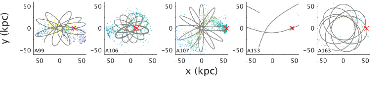
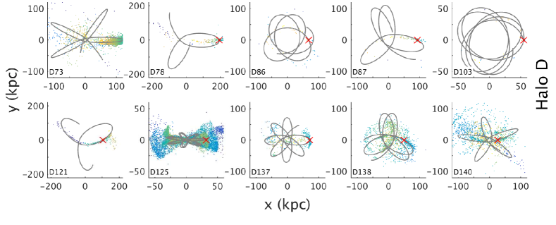
Figure 19: Same as Fig. 4 but with the remaining streams streams with at least 500 dark matter particles that were not shown in that figure.

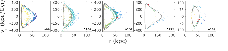
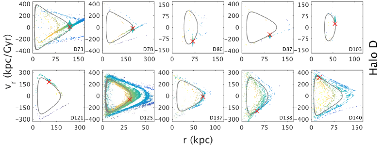
Figure 20: Same as Fig. 5 but with the remaining streams streams with at least 500 dark matter particles that were not shown in that figure.

Appendix C Numerical parameters for Kuzmin-Kutuzov potential

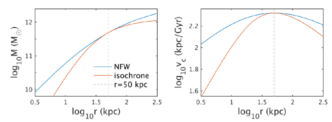
Figure 21: Enclosed mass and circular velocity curves for the best fitting NFW profile to halo Aq-D, and the isochrone potential that matches the enclosed mass and slope at $r_{\textrm{fix}}=50$ kpc.

To set the numerical values of the parameters of the axisymmetric Staeckel potential used in the experiments of Section  4 we proceed as follows. We first set up the isochrone potential by choosing a radius $r_{\textrm{fix}}$ at which the enclosed mass and its slope equals that of the best-fitting NFW potential for the Aquarius halos. This ensures that around $r_{\textrm{fix}}$ the (spherically averaged) mass distributions are similar. We choose $r_{\textrm{fix}}=50$ kpc because most of the streams we study are located around $50$-$100$ kpc from the halo centre. Having chosen $r_{\text{fix}}$, we first match the slope of the mass profile and then proceed to set the enclosed mass. The logarithmic slope $\kappa$ is

$$\kappa_{\textrm{NFW}}(x)\equiv\frac{{\rm d}\log M_{\textrm{NFW}}(x)}{{\rm d}\log x}$$ (12)

with $x=r/r_{\textrm{s}}$ and $r_{\textrm{s}}$ the scale radius of the NFW potential such that $M_{\textrm{NFW}}(r_{\textrm{s}})=M_{\textrm{s}}$. The condition of equal slopes at $r_{\textrm{fix}}$ is

$$\kappa_{\textrm{NFW}}(r_{\textrm{fix}}/r_{\textrm{s}})=\kappa_{\textrm{iso}}(r_{\textrm{fix}}/r_{\textrm{iso}}),$$ (13)

which we can invert to find $r_{\textrm{iso}}$. The scale mass $M_{\textrm{iso}}$ ensures the enclosed mass is equal at $r_{\textrm{fix}}$

$$M_{\textrm{s}}\frac{A_{\textrm{NFW}}(r_{\textrm{fix}}/r_{\textrm{s}})}{A_{\textrm{NFW}}(1)}=M_{\textrm{iso}}\frac{A_{\textrm{iso}}(r_{\textrm{fix}}/r_{\textrm{iso}})}{A_{\textrm{iso}}(1)},$$ (14)

where $A_{i}$ are the normalised radial mass profiles for the used potentials. In Fig. 21 we show the result of our fitting procedure for halo Aq-D. The overall mass and velocity profiles differ significantly outside $r\sim r_{\textrm{fix}}$.

The next step in setting up the axisymmetric Kuzmin-Kutuzov potential is to use Eqs. (11) to determine its characteristic parameters. This requires some measurement of the shape of the Aquarius halos, and we use the axis ratios determined using the reduced moment of inertia tensor at $r_{\textrm{fix}}=50$ kpc by Vera-Ciro et al. (2011), and which closely follow the isodensity contours. Since Aq-A and Aq-D halos are more prolate, we define an axisymmetric equivalent of the axis ratio of the density $q_{\rho}$ as

$$q_{\rho}=\dfrac{2a}{b+c},$$ (15)

where $a$, $b$ and $c$ are the major, intermediate and minor axis lengths. For halo Aq-D $q_{\rho}(50\leavevmode\nobreak\ {\rm kpc})=1.53$ ($q_{\rho}=1.39$ when the axis ratios $b/a$ and $c/a$ are determined at 100 kpc).

The density profile of the Kuzmin-Kutuzov potential is given by (Dejonghe & de Zeeuw 1988):

$$\rho_{\textrm{K}}(\lambda,\nu)=\frac{M_{\textrm{K}}\,c_{\textrm{K}}^{2}}{4\pi}\frac{\lambda\nu+a_{\textrm{K}}^{2}\left(\lambda+3\sqrt{\lambda\nu}+\nu\right)}{\left(\lambda\nu\right)^{3/2}\left(\sqrt{\lambda}+\sqrt{\nu}\right)^{3}}.$$ (16)

We can use this expression to solve numerically for the value of $q_{\textrm{K}}$ such that the isodensity-contour at $R=50$ kpc has the desired axis ratio $q_{\rho}$. This results in $q_{\textrm{K}}=1.87$ for halo Aq-D. Note that for this value of $q_{\textrm{K}}$ we find $q_{\rho,\textrm{K}}=1.44$ at 100 kpc for the Kuzmin-Kutuzov potential, which is also not too far off from the value of $q_{\rho}(100\leavevmode\nobreak\ {\rm kpc})=1.39$ measured for Aq-D.

Appendix D Fitting algorithm

When the individual wraps of a stream are sufficiently distinct in angle space, we can fit straight lines to these. Their slopes can then be compared to those obtained when fitting in frequency space. In Section 3, we derived the angle distributions for streams assuming a spherical potential. These distributions are rather noisy and make the process of fitting straight lines non-trivial and complex. Therefore, we proceed to describe now in detail the steps that we take to measure the slopes in angle space.

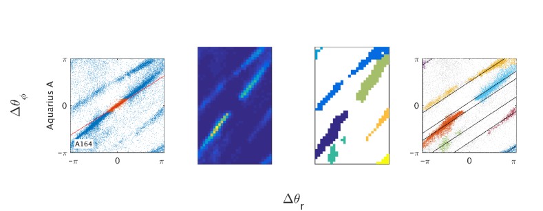
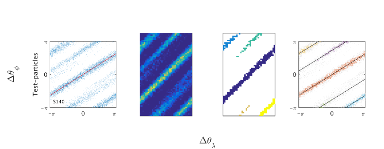
Figure 22: Examples of the straight lines fitting routine for stream A164 (top panels) and the test particle simulations’ S140. In the left panel we show the stream in angle space with possible bound particles in red and the straight line obtained by fitting the frequency distribution. The second panel shows the streams in bins, where the axis have been scaled such that the streams are oriented at 45 deg. The third panel shows the groupings found by the pattern filling algorithm. The last panel shows the resulting straight lines determined using parallel fitting.

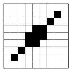
Figure 23: Pattern used to link pixels in the angle-space image of the stream.

In Fig. 22 we show two examples: stream A164 and the test-particle simulations stream S140 as they are being fitted. In case of the Aquarius halos, we first use the binding energies of the particles in the stream to find the most bound particle and then centre angle and frequency space on this particle. If there is no bound structure, the centre is put at the location of the highest density in angle space. We generously remove the progenitor and particles in its surroundings by computing the total binding energy with a much higher mass per particle ($\sim 4$). These bound particles are marked in red in the top-left panel of Fig. 22.

In the next step we fit a straight line to the remaining particles in each independent projection of frequency space using a simple least squares method. We show this line for the $r$-$\phi$ projection of angle space in the left panels of Fig. 22. We then bin the data of this angle space projection in $N$ bins horizontally and $N/S(\Delta\Omega_{\phi})$ vertically, where $N=40$ for the test-particle streams and $N=30$ for the Aquarius streams, unless there are fewer than 100 particles remaining. We then ‘clean’ this image by emptying the bins that have fewer counts than the median of non-empty pixels. This is done twice to generate enough contrast w.r.t. ’background’ of particles between the streams for the Sculptor progenitors, and only once for the thinner Carina progenitors (e.g. Fig. 12).

We group the particles by connecting pixels that fall within the pattern of Fig. 23, which is elongated in the same direction as the stream, which is on an angle of 45 degrees if it follows the frequency distribution. Some parallel streams may be ‘connected’ at a single pixel, and the algorithm keeps them separate by not combining groups that individually had more than 25 connected pixels. This procedure results in the groups shown in the third column of Fig. 22 with different colours. It is clear from the top row that sometimes structures are grouped together that should not be connected, but it is difficult to completely prevent this from happening without removing too many particles from the streams.

We then use a least-squares fit for parallel lines with different offsets. The result is optimised by running the full fitting procedure twice, because we can then use the slope fitted to the angles found in the first iteration when binning angle space. To estimate the errors in the fitting we bootstrap the data 200 times, which was found to be enough to get a reasonable estimate of the errors, although this does not fully reflect the error when the wraps in angle space overlap or if they are not on parallel lines.

References

- Allgood et al. (2006) Allgood, B., Flores, R. A., Primack, J. R., et al. 2006, MNRAS, 367, 1781
- Binney (2008) Binney, J. 2008, MNRAS, 386, L47
- Binney (2012) Binney, J. 2012, MNRAS, 426, 1324
- Binney & Tremaine (2008) Binney, J. & Tremaine, S. 2008, Galactic Dynamics: Second Edition (Princeton University Press)
- Bonaca et al. (2014) Bonaca, A., Geha, M., Küpper, A. H. W., et al. 2014, ApJ, 795, 94
- Bovy (2014) Bovy, J. 2014, ApJ, 795, 95
- Bower et al. (2006) Bower, R. G., Benson, A. J., Malbon, R., et al. 2006, MNRAS, 370, 645
- Boylan-Kolchin et al. (2009) Boylan-Kolchin, M., Springel, V., White, S. D. M., Jenkins, A., & Lemson, G. 2009, MNRAS, 398, 1150
- Buist & Helmi (2015) Buist, H. J. T. & Helmi, A. 2015, ArXiv e-prints
- Carlberg (2013) Carlberg, R. G. 2013, ApJ, 775, 90
- Choi et al. (2007) Choi, J.-H., Weinberg, M. D., & Katz, N. 2007, MNRAS, 381, 987
- Choi et al. (2009) Choi, J.-H., Weinberg, M. D., & Katz, N. 2009, MNRAS, 400, 1247
- Cooper et al. (2010) Cooper, A. P., Cole, S., Frenk, C. S., et al. 2010, MNRAS, 406, 744
- Dalton et al. (2012) Dalton, G., Trager, S. C., Abrams, D. C., et al. 2012, in Society of Photo-Optical Instrumentation Engineers (SPIE) Conference Series, Vol. 8446, Society of Photo-Optical Instrumentation Engineers (SPIE) Conference Series, 0
- de Jong et al. (2012) de Jong, R. S., Bellido-Tirado, O., Chiappini, C., et al. 2012, in Society of Photo-Optical Instrumentation Engineers (SPIE) Conference Series, Vol. 8446, Society of Photo-Optical Instrumentation Engineers (SPIE) Conference Series, 0
- de Zeeuw (1985) de Zeeuw, T. 1985, MNRAS, 216, 273
- Dejonghe & de Zeeuw (1988) Dejonghe, H. & de Zeeuw, T. 1988, ApJ, 333, 90
- Einasto (1965) Einasto, J. 1965, Trudy Astrofizicheskogo Instituta Alma-Ata, 5, 87
- Eyre & Binney (2009) Eyre, A. & Binney, J. 2009, MNRAS, 400, 548
- Eyre & Binney (2011) Eyre, A. & Binney, J. 2011, MNRAS, 413, 1852
- Font et al. (2011) Font, A. S., Benson, A. J., Bower, R. G., et al. 2011, MNRAS, 417, 1260
- Fox (2012) Fox, M. 2012, M. Phys. thesis, Univ. Oxford
- Franx et al. (1991) Franx, M., Illingworth, G., & de Zeeuw, T. 1991, ApJ, 383, 112
- Gibbons et al. (2014) Gibbons, S. L. J., Belokurov, V., & Evans, N. W. 2014, MNRAS, 445, 3788
- Goldstein (1950) Goldstein, H. 1950, Classical mechanics (Addison-Wesley Publishing Company)
- Gómez et al. (2015) Gómez, F. A., Besla, G., Carpintero, D. D., et al. 2015, ApJ, 802, 128
- Gómez & Helmi (2010) Gómez, F. A. & Helmi, A. 2010, MNRAS, 401, 2285
- Gómez et al. (2010) Gómez, F. A., Helmi, A., Brown, A. G. A., & Li, Y.-S. 2010, MNRAS, 408, 935
- Helmi & de Zeeuw (2000) Helmi, A. & de Zeeuw, P. T. 2000, MNRAS, 319, 657
- Helmi & White (1999) Helmi, A. & White, S. D. M. 1999, MNRAS, 307, 495
- Helmi & White (2001) Helmi, A. & White, S. D. M. 2001, MNRAS, 323, 529
- Henon (1959) Henon, M. 1959, Annales d’Astrophysique, 22, 126
- Ibata et al. (2001) Ibata, R., Lewis, G. F., Irwin, M., Totten, E., & Quinn, T. 2001, ApJ, 551, 294
- Jin & Lynden-Bell (2007) Jin, S. & Lynden-Bell, D. 2007, MNRAS, 378, L64
- Johnston (1998) Johnston, K. V. 1998, ApJ, 495, 297
- Johnston & Bullock (2004) Johnston, K. V. & Bullock, J. S. 2004, in Astronomical Society of the Pacific Conference Series, Vol. 327, Satellites and Tidal Streams, ed. F. Prada, D. Martinez Delgado, & T. J. Mahoney, 213
- Johnston et al. (1999) Johnston, K. V., Zhao, H., Spergel, D. N., & Hernquist, L. 1999, ApJ, 512, L109
- Kaasalainen & Binney (1994) Kaasalainen, M. & Binney, J. 1994, MNRAS, 268, 1033
- Koposov et al. (2012) Koposov, S. E., Belokurov, V., Evans, N. W., et al. 2012, ApJ, 750, 80
- Koposov et al. (2010) Koposov, S. E., Rix, H.-W., & Hogg, D. W. 2010, ApJ, 712, 260
- Küpper et al. (2010) Küpper, A. H. W., Kroupa, P., Baumgardt, H., & Heggie, D. C. 2010, MNRAS, 401, 105
- Küpper et al. (2012) Küpper, A. H. W., Lane, R. R., & Heggie, D. C. 2012, MNRAS, 420, 2700
- Law et al. (2005) Law, D. R., Johnston, K. V., & Majewski, S. R. 2005, ApJ, 619, 807
- Law & Majewski (2010) Law, D. R. & Majewski, S. R. 2010, ApJ, 714, 229
- Lowing et al. (2015) Lowing, B., Wang, W., Cooper, A., et al. 2015, MNRAS, 446, 2274
- Magorrian (2014) Magorrian, J. 2014, MNRAS, 437, 2230
- Martin et al. (2014) Martin, N. F., Ibata, R. A., Rich, R. M., et al. 2014, ApJ, 787, 19
- McGill & Binney (1990) McGill, C. & Binney, J. 1990, MNRAS, 244, 634
- McMillan & Binney (2008) McMillan, P. J. & Binney, J. J. 2008, MNRAS, 390, 429
- Merritt & Valluri (1999) Merritt, D. & Valluri, M. 1999, AJ, 118, 1177
- Miralda-Escude & Schwarzschild (1989) Miralda-Escude, J. & Schwarzschild, M. 1989, ApJ, 339, 752
- Navarro et al. (1996) Navarro, J. F., Frenk, C. S., & White, S. D. M. 1996, ApJ, 462, 563
- Navarro et al. (1997) Navarro, J. F., Frenk, C. S., & White, S. D. M. 1997, ApJ, 490, 493
- Navarro et al. (2010) Navarro, J. F., Ludlow, A., Springel, V., et al. 2010, MNRAS, 402, 21
- Ngan & Carlberg (2014) Ngan, W. H. W. & Carlberg, R. G. 2014, ApJ, 788, 181
- Peñarrubia et al. (2012) Peñarrubia, J., Koposov, S. E., & Walker, M. G. 2012, ApJ, 760, 2
- Perryman et al. (2001) Perryman, M. A. C., de Boer, K. S., Gilmore, G., et al. 2001, A&A, 369, 339
- Power et al. (2003) Power, C., Navarro, J. F., Jenkins, A., et al. 2003, MNRAS, 338, 14
- Sanders (2012) Sanders, J. 2012, MNRAS, 426, 128
- Sanders & Binney (2013a) Sanders, J. L. & Binney, J. 2013a, MNRAS, 433, 1813
- Sanders & Binney (2013b) Sanders, J. L. & Binney, J. 2013b, MNRAS, 433, 1826
- Sanders & Binney (2014) Sanders, J. L. & Binney, J. 2014, MNRAS, 441, 3284
- Sanders & Binney (2015) Sanders, J. L. & Binney, J. 2015, MNRAS, 447, 2479
- Sanderson et al. (2014) Sanderson, R. E., Helmi, A., & Hogg, D. W. 2014, in IAU Symposium, Vol. 298, IAU Symposium, ed. S. Feltzing, G. Zhao, N. A. Walton, & P. Whitelock, 207–212
- Springel et al. (2008) Springel, V., Wang, J., Vogelsberger, M., et al. 2008, MNRAS, 391, 1685
- Strigari (2013) Strigari, L. E. 2013, Phys. Rep., 531, 1
- Tremaine (1999) Tremaine, S. 1999, MNRAS, 307, 877
- Vera-Ciro & Helmi (2013) Vera-Ciro, C. & Helmi, A. 2013, ApJ, 773, L4
- Vera-Ciro et al. (2011) Vera-Ciro, C. A., Sales, L. V., Helmi, A., et al. 2011, MNRAS, 416, 1377
- Wang et al. (2011) Wang, J., Navarro, J. F., Frenk, C. S., et al. 2011, MNRAS, 413, 1373
- Warren et al. (1992) Warren, M. S., Quinn, P. J., Salmon, J. K., & Zurek, W. H. 1992, ApJ, 399, 405
- Yoon et al. (2011) Yoon, J. H., Johnston, K. V., & Hogg, D. W. 2011, ApJ, 731, 58