On the robustness of the pendulum model for large-amplitude longitudinal oscillations in prominences

Abstract

Large-amplitude longitudinal oscillations (LALOs) in prominences are spectacular manifestations of the solar activity. In such events nearby energetic disturbances induce periodic motions on filaments with displacements comparable to the size of the filaments themselves and with velocities larger than $20{\mathrm{\,km\;s^{-1}}}$. The pendulum model, in which the gravity projected along a rigid magnetic field is the restoring force, was proposed to explain these events. However, it can be objected that in a realistic situation where the magnetic field reacts to the mass motion of the heavy prominence, the simplified pendulum model could be no longer valid. We have performed non-linear time-dependent numerical simulations of LALOs considering a dipped magnetic field line structure. In this work we demonstrate that for even relatively weak magnetic fields the pendulum model works very well. We therefore validate the pendulum model and show its robustness, with important implications for prominence seismology purposes. With this model it is possible to infer the geometry of the dipped field lines that support the prominence.

1. Introduction

Large-amplitude oscillations (LAOs) of prominences are recently attracting more attention in the solar physics community. The number of reported events is increasing as the current telescope capabilities allow for continuous full Sun monitoring. LAOs are motions involving speeds larger than $20{\mathrm{\,km\;s^{-1}}}$ according to the classification of Oliver & Ballester (2002). These speeds are larger than the local sound speed in the cool prominence plasma, typically $c_{\mathrm{s}}\sim 10{\mathrm{\,km\;s^{-1}}}$. Thus, LAOs involve supersonic motions and non-linear effects are expected.

LAOs are typically divided in two kinds of motions: longitudinal and transverse with respect to the spine of the filament (see a review by Tripathi et al., 2009). In this work we focus exclusively on the large-amplitude longitudinal oscillations (LALOs) case. These motions were first reported by Jing et al. (2003) followed by two more publications by Jing et al. (2006) and Vršnak et al. (2007). In these works the authors reported five LALOs events where the filament plasma move almost parallel to their spines. More recently Zhang et al. (2012) reported an oscillation at the limb showing that the motion is along the prominence dipped magnetic field lines. More LALOs observations were reported and characterized in later work (Li & Zhang, 2012; Bi et al., 2014; Shen et al., 2014; Luna et al., 2014). In all the LALOs reported so far the periods range from 40 to 100 minutes and the amplitudes are between $20{\mathrm{\,km\;s^{-1}}}$ to $100{\mathrm{\,km\;s^{-1}}}$. In LALOs the prominence threads move parallel to themselves indicating that the motion is along the magnetic field. Luna et al. (2014) demonstrated that in the considered event the motion formed $25^{\circ}$ with respect to the filament spine. That orientation coincided with the typical observed orientations of the magnetic field of filaments (see e.g., Leroy et al., 1983, 1984). Thus, all above evidences suggest that LALOs are actually oscillations along the magnetic field.

The nature of LALOs is currently a matter of discussion since, in principle, several forces could act as the restoring force. Based on 1D numerical simulations, Luna & Karpen (2012) proposed the pendulum model to explain LALOs, where the restoring force is the gravity projected along the magnetic field lines. These authors discarded the magnetic origin of the restoring force because the Lorentz force is always perpendicular to the magnetic field and does not affect the longitudinal motion. Similarly, the numerical simulations presented by Luna & Karpen (2012) show that the gas pressure gradient force is not important and that the nature of LALOs is not magnetosonic. These results were confirmed by other 1D simulations by Zhang et al. (2012, 2013). Luna et al. (2012) performed an analytical study of the influence of the magnetic field curvature on linear longitudinal oscillations. It was found that the longitudinal oscillations are in general a combination of the pendulum and the slow modes. However, for typical prominence parameters the contribution of the slow modes is very small confirming the findings of previous studies. All these results support the pendulum model for the LALOs.

The main drawback of the 1D modeling is that the magnetic field is assumed rigid and the motion of the plasma perfectly follows the field lines. In this regime the magnetic field does not react to the motion of the plasma. However, the heavy mass of the prominence and the non-zero value of the plasma-$\beta$ could make the role of the magnetic field more important and influence the motion of threads (Li & Zhang, 2012). For example, the mass could change dynamically the magnetic structure producing non-linear coupling of the longitudinal and transverse motions and the pendulum model might be no longer valid. Recently, Terradas et al. (2013) studied the different modes of oscillations of a prominence embedded in a 2D structure in the linear regime. They used a realistic scenario where the magnetic field reacts to the plasma motion. The authors found evidences that the longitudinal motion is affected by the gravity but also by the gas pressure. However, the authors placed the prominence in a very high position where the field lines are essentially flat and convex-downwards. At such position, the longitudinal motion is strongly influenced by the slow modes as was found in Luna et al. (2012).

Due to the potential applicability for prominence seismology, it is necessary to validate or to discard the pendulum model. In this study we demonstrate that the pendulum model is robust, with non-linear 2D time-dependent numerical simulations. We prove that the period of the oscillations depends exclusively on the radius of curvature of the dipped field lines and that the longitudinal and transverse motions (relative to the magnetic field) are not strongly coupled. The back reaction of the magnetic field is small when LALOs are present and the restoring force is the projection of the gravity along the magnetic field lines.

2. The numerical experiment

The aim of the numerical experiment is to reproduce the LALOs observed in filaments. In those events nearby energetic disturbances perturb an existing filament from the side, probably along the filament-channel magnetic structure. The hot plasma produced at the energetic event flows along the magnetic field lines pushing an already formed prominence. In order to have a prominence we instantaneously load a force free magnetic structure with a prominence mass. Initially, such a configuration is not in force equilibrium. We then let the system evolve in order to have a relatively relaxed configuration. The amplitude of the motions of the system decreases with time but the velocity field does not disappear completely. Once we reach a relatively relaxed situation we instantaneously apply a velocity perturbation along the magnetic field of the prominence in order to mimic a typical observed excitation event such as a jet or a small flare. The velocity perturbation is placed over the almost relaxed prominence with a speed of $20{\mathrm{\,km\;s^{-1}}}$, typical for LALOs.

In the relaxation phase, the initial configuration consists of a force-free magnetic field described in Terradas et al. (2013). It represents a symmetric double arcade given by Equations (1) and (2) and plotted in Figure 1.

$$\frac{B_{x}(x,z)}{B_{0}} = \cos k_{1}x\,e^{-k_{1}(z-z_{0})}-\cos k_{2}x\,e^{-k_{2}(z-z_{0})}~{},$$ (1)

$$\frac{B_{z}(x,z)}{B_{0}} = -\sin k_{1}x\,e^{-k_{1}(z-z_{0})}+\sin k_{2}x\,e^{-k_{2}(z-z_{0})}~{}.$$ (2)

This structure has dips closer to the surface, where we initially place the prominence mass. The depth of the dips decreases monotonically from bottom to top positions and the curvature at the central position of the field lines changes from concave upwards to convex downwards forming a overlying arcade of loops.

The magnetic field has a null point at $(0,z_{0})$ that we have placed outside the numerical domain by taking $z_{0}=-2{\mathrm{\,Mm}}$. In addition, placing the null point bellow the numerical domain we avoid partially the non realistic region of very high plasma-$\beta$ (ratio of gas pressure to magnetic pressure) surrounding the null. Both pressures change dynamically with time, but the plasma-$\beta$ is always constrained to $\beta<0.4$ in all the numerical domain. We have considered the parameters $B_{0}=30{\mathrm{\,G}}$ and $k_{1}=k_{2}/3=\pi/100{\mathrm{\,Mm}}^{-1}$. At the central position of the structure the magnetic field strength is $3.3{\mathrm{\,G}}$ at $z=0$ and reaches a maximum of $11.5{\mathrm{\,G}}$ at $z=15.5{\mathrm{\,Mm}}$. Beyond this point the field strength decreases with height. This point coincides with the change of curvature of the field lines. Thus, below $z=15.5{\mathrm{\,Mm}}$ the magnetic structure has dips whereas above this point the structure is an arcade of loops. The numerical domain consists of a box of $800\times 800$ points and $100\times 100{\mathrm{\,Mm}}$, with a spatial resolution of 125 km. We assume open boundary conditions for the top and the two side boundaries. At the bottom boundary, line-tying is considered by imposing current free conditions and zero velocities as in Terradas et al. (2013).

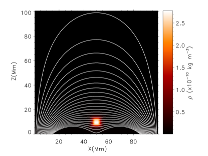
Figure 1.— Initial configuration consisting of a stratified corona and a force-free magnetic field given by Equations (1) and (2) and an initial density and temperature prominence perturbation. For the force-free magnetic configuration we have imposed $B_{0}=30\,\mathrm{G}$, $k_{1}=k_{2}/3=\pi/100{\mathrm{\,Mm}}^{-1}$, and $z_{0}=-2{\mathrm{\,Mm}}$. A selected set of field lines have been plotted as white lines. The color field represents the density at the prominence and corona. The density of the internal part of the prominence is $100$ times the density of the corona.

The coronal plasma is assumed initially stratified with a uniform million degree temperature, $T_{c}=10^{6}\,\mathrm{K}$. The prominence is placed on the structure by perturbing the coronal atmosphere with a temperature of the form

$$T(x,z)=T_{c}+\delta T_{0}\,e^{-\frac{(x-x_{T})^{4}}{w_{x}^{4}}-\frac{(z-z_{T})^{4}}{w_{z}^{4}}}$$ (3)

where $(x_{T},z_{T})=(50,10){\mathrm{\,Mm}}$ is the position of the center of the pulse and $w_{x}=w_{z}=10{\mathrm{\,Mm}}$ are the widths of the perturbation in $x$- and $z$-directions respectively. The temperature at the central position of the prominence is $T=10.000\,\mathrm{K}$ and $\delta T_{0}$ is selected accordingly to $-0.99\times 10^{6}\,\mathrm{K}$. The initial temperature perturbation has a quartic dependence in the exponent in order to have a large region of cool and dense plasma. The pressure is unperturbed and equal to that of the ambient corona. The density of the perturbation is computed accordingly to the ideal gas law (see Fig. 1). In this situation, the gas pressure along the horizontal direction is uniform, $\rho_{\mathrm{c}}(z)\,T_{\mathrm{c}}(z)=\rho_{\mathrm{p}}(x,z)\,T_{\mathrm{p}}(x,z)$.

We numerically solve the ideal MHD equations in the above scenario by using our recently developed MANCHA code (Khomenko et al., 2008; Felipe et al., 2010; Khomenko & Collados, 2012; Khomenko et al., 2014). MANCHA solves the time dependent nonlinear problem given initial conditions. The relaxation phase is not relevant for this study, but it is sufficiently interesting to be briefly described. The initial configuration is not in equilibrium and the weight of the prominence mass is not compensated by the magnetic structure or gas pressure gradients. The prominence plasma rapidly starts to fall and collapses, increasing its internal pressure. After some time the collapse ceases producing a shock wave that propagates along the magnetic field lines at both sides of the prominence. These shocks bounce at the field footpoints moving back again to the prominence. The shocks travel between the two footpoints, and the prominence oscillates vertically producing again more shocks by the same process. After $7000{\mathrm{\,seconds}}$ the prominence is more or less relaxed into a dynamical equilibrium. At this point vertical oscillations and waves along the magnetic field remain but the speeds involved are below $5{\mathrm{\,km\;s^{-1}}}$. It is important to note that we include the remnant velocities in the next phase where we add the longitudinal perturbation to the already existing velocity field. The resulting dynamics will not be strongly influenced by these remnant motions.

3. Large-Amplitude Longitudinal Perturbation and Oscillations

Once the prominence is sufficiently relaxed we perturb the resulting configuration with a velocity field along the magnetic structure, namely

$$\vec{v}_{0}=v_{0}\frac{\vec{B}_{0}}{B_{0}}e^{-\frac{(x-x_{T})^{4}}{w_{vx}^{4}}-\frac{(z-z_{T})^{4}}{w_{vz}^{4}}}\,,$$ (4)

in order to excite longitudinal motions. We have considered this time as $t=0$. The relaxation phase has $t<0$, while $t\geq 0$ is taken after the longitudinal velocity perturbation. $\vec{B}_{0}$ is the magnetic field at the end of the relation phase or at $t=0$. The perturbation has $w_{vx}=3\,w_{x}$ and $w_{vz}=3\,w_{z}$, much larger than the initial temperature perturbation in order to excite oscillations of the cool plasma and in their surrounding. The perturbed initial velocity is set to $v_{0}=20{\mathrm{\,km\;s^{-1}}}$ which is in the range of large-amplitude oscillations. Due to the dimensions of the considered structure, larger initial velocities produce drainage of cool plasma on the sides of the structure.

In Figure 2 we have plotted a four panel time sequence of the density and the magnetic field.

Figure 2.— Time sequence evolution of the plasma (colors) and the magnetic structure (white lines) at four times. Panel (a) shows the initial configuration at $t=0$ when the longitudinal perturbation is applied. In (b) we see the prominence almost reaching the maximum elongation of its displacement. In (c) the phase differences between different parts of the structure is clear. In (d) a clear zig-zag motion of the prominence is shown. The color represents the density of the prominence.

In Figure 2a the almost relaxed prominence is plotted. In contrast with the non-equilibrium initial situation (Fig. 1) the density is now more vertically elongated because the cool plasma has deformed the initial magnetic field. We perturb the system with the velocity of Equation (4) and the whole prominence material starts to move towards the increasing values of $x$-coordinate following clearly the magnetic field lines. The velocity also decreases with time and after approximately $10{\mathrm{\,minutes}}$ most of the prominence reaches the maximum displacement (Fig. 2b) and the motion reverses. However, the bottom parts of the prominence reverse the direction of motion slightly before the rest of the structure. The motion along the vertical structure is different and the phase difference becomes important, as it is apparent in Figure 2c. At this time the bottom part moves rightward and the central part leftwards with the top part considerably delayed. The increase in the delay between the different parts of the structure seems gradual. The last panel (Fig. 2d) shows very well that the motion between different parts of the structure becomes out of phase with opposite directions of motion. This indicates that the plasma moves along the magnetic field with different periods of oscillation. The zig-zag structure resembles the motion of the apparent tornado structure observed with the SDO/AIA, as reported by Su et al. (2012). From the figure it is clear that the density changes with time in reaction to both longitudinal and transverse movements.

The magnetic field structure also changes during the temporal evolution. In the figure, the white solid lines are a set of selected field lines at different times and the white dashed lines represent the magnetic field at $t=0$ (Fig. 2a). In the first period the magnetic field changes slightly (Figs. 2b and 2c) but rapidly recovers the initial configuration and remains more or less unchanged for the rest of the temporal evolution (see Fig. 2d). In the time-dependent evolution we do not find a swaying motion of the magnetic structure. In contrast, the magnetic structure remains more or less unchanged except for some small-amplitude vertical oscillations. We conclude that the motion of the plasma mainly follows the magnetic field lines.

We see that different parts of the structure oscillate with different frequencies forming a continuous spectrum (Goossens et al., 1985; Terradas et al., 2013). This behavior makes the spectral study of the motion complicated. In addition, these oscillations are essentially non-linear and the plasma is subject to important advection. In our fluid, the frozen-in condition applies because we consider it to be perfectly conducting. Thus, it is necessary to advect every field line considered in order to catch the longitudinal and transverse motions of the plasma. The bottom line-tying boundary conditions imply that the magnetic field is unperturbed during the temporal evolution. Thus, any field line starting at the bottom boundary follows the plasma motion simplifying the study of the oscillations. We select a large set of equally spaced field lines starting at the bottom. These field lines cross the central axis ($x=0$) with approximate separations of $0.25{\mathrm{\,Mm}}$. The lines plotted in Figure 2 are only a small subset of the field lines considered in the following analysis.

We have computed the longitudinal and transverse motions of the center of mass as

$$v_{\parallel i}(t)=\int v_{\parallel}(s_{i},t)\rho(s_{i},t)ds_{i}/\int\rho(s_{i},t)ds_{i}\,,$$ (5)

$$v_{\perp i}(t)=\int v_{\perp}(s_{i},t)\rho(s_{i},t)ds_{i}/\int\rho(s_{i},t)ds_{i}\,.$$ (6)

The $i$-index corresponds to the field line considered and $s_{i}$ is the coordinate along the field line $i$ that depends implicitly on the time, $t$. The integrands $v_{\parallel}(s_{i},t)$, $v_{\perp}(s_{i},t)$ and $\rho(s_{i},t)$ are the longitudinal velocity, transverse velocity and density along the field line $i$ respectively. These velocities are plotted in Figure 3 for the different field lines.

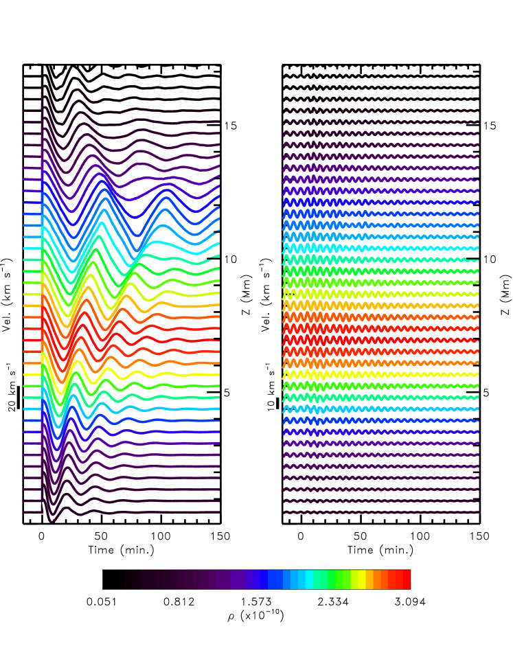
Figure 3.— Plot of the longitudinal (left panel) and transverse (right panel) motions of the center of mass for every field line considered. In this plot the vertical axis represents an arbitrary scale. On each panel a velocity scale is plotted. This plot is convenient to show the relative oscillation phase at the different heights of the structure.

The left vertical axis shows the velocity scale. For comparison, the right vertical axis shows the $z_{i}$-coordinate at the central position $x=0$ of the field lines at $t=0$. In a linear situation this is equivalent to studying the velocities along the vertical axis at $x=0$. We have plotted the temporal evolution of the velocities from $t=-15{\mathrm{\,minutes}}$ to $t=150\min$. Before $t=0$ we clearly see the velocities of the relaxation phase at the right panel. At the relaxation phase the central positions of the prominence oscillate vertically because we place the mass centered at the structure. We see that the longitudinal velocities are zero (left panel) but there are clear oscillations along the vertical direction (right panel). At $t=0$ we impose the instantaneous velocity perturbation that produces a sudden increase of the longitudinal velocity to $20{\mathrm{\,km\;s^{-1}}}$, but no significant changes to the transverse motion. The different nature of the longitudinal and transverse oscillations is also clear in their very different periods of oscillation. We define the density at the center of mass of each field line as ${\rho_{CM}}_{i}(t)=\rho({s_{CM}}_{i},t)$ being ${s_{CM}}_{i}$ the position of the center of mass along the field line $i$. The color coding is computed as the temporal average of ${\rho_{CM}}_{i}(t)$. With this color coding we can identify the oscillation corresponding to coronal or prominence plasma. The longitudinal period increases monotonically from the bottom positions up to $z\sim 11{\mathrm{\,Mm}}$. This range of heights includes almost all the prominence. Above $z\sim 11{\mathrm{\,Mm}}$ the period of the oscillations decreases. From the figure we see that the longitudinal velocity at denser plasma shows a triangular shape with peaked maximums and minimums instead of a sinusoidal shape. This could be related to the non-linearity of the oscillations.

The longitudinal oscillations show a significant damping (Fig. 3a) in contrast to the weak damping of the transverse motions (Fig. 3b). LALOs show different damping times for different parts of the structure. The plasma oscillations at the bottom parts of the structure are damped quicker than at the top parts. In order to study the convergence of the numerical solutions, we have performed a check repeating our simulations with a decreased resolution of 500 and 250 km grid sizes. We found that at all resolutions the simulations show a similar damping scale, with slightly larger damping for larger grid sizes and identical periods. Therefore, these tests demonstrate that our simulations have converged. We may speculate that a kind of numerical phase-mixing is probably occurring for LAL oscillations, mimicking a real process that may occur on the Sun. LALOs at different field lines have different frequencies because they have different field line curvature. Then two adjacent field lines at the numerical grid lose their relative coherence and due to the numerical viscosity the motion tends to be canceled by stress. The numerical viscosity depends on the grid size. However, the convergence test has shown that we are very far from reaching realistic values of dissipation because the models with different resolution exhibit similar damping. Thus, significantly better grids are required to resolve the transition region surrounding the oscillating thread and to avoid the enhanced numerical viscosity phase-mixing. This will be addressed in a future work using a new module of MANCHA with Adaptive Mesh Refinement. The study of the damping mechanism is out of the scope of this work. However, understanding the nature of this damping is also important for LALOs and it will be considered in a future publication.

The transverse velocities in Figure 3 (right panel) show an amazingly regular and coherent motion. After the perturbation ($t>0$), there is an alteration of the regular pattern, but the system quickly recovers its very regular motion. There are no important phase differences, and the oscillation periods are very similar ($5.4{\mathrm{\,minutes}}$ in all field lines analyzed). This behavior suggests that the transverse motions is a global normal mode of the structure. However, one of the most important results is that there are no transverse motions associated to the longitudinal motion.The back reaction of the magnetic field should have produced displacements perpendicular to the magnetic field with the same or half period than the longitudinal motion. However, this is not observed in Figure 3 or in the spectral analysis of the curves.

We have analyzed the periods of oscillations at every field line considered in the two polarization directions. The results are plotted in Figure 4.

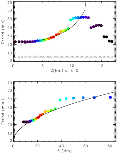
Figure 4.— Scatter plot of the periods of oscillation as function of $z$-position of the field lines dips, as in Figure 3 (top panel), and radius of curvature (bottom panel) of the field lines. The radius of curvature is computed numerically along the field lines and averaged in space and time. The radius of curvature for every field line is spatially averaged in $3{\mathrm{\,Mm}}$ along the line centered at the dip for every snapshot. This spatially averaged radii are also temporally averaged in all the simulation time $t\geq 0$. The color code is identical to Fig. 3.

The longitudinal period increases with height (top panel) as we have discussed previously. The increase is monotonic but above $z\sim 9.5{\mathrm{\,Mm}}$ the behavior changes, in agreement with the visual impression from Figure 3. In the figure we have plotted the theoretical period, $P$, of the mass loaded into the deformed structure (solid line) using the pendulum model expression from Luna & Karpen (2012),

$$P=2\pi\sqrt{\frac{R}{g}}\,,$$ (7)

where $R$ is the radius of curvature of the dipped portion of the field lines and $g=274\,\mathrm{m\,s^{-2}}$ is the solar gravity acceleration. We have computed the radius of the curvature at the center of the dipped portion of the field lines. These radii slightly change in reaction to the mass motion. We therefore have considered the temporal average of the radii. We can see an excellent agreement between the time-dependent simulations and the pendulum model in the range $z=3-9.5{\mathrm{\,Mm}}$ that includes most of the prominence mass. Above $z\sim 9.5{\mathrm{\,Mm}}$ there is no agreement with the model. Above this point the gas pressure gradient contributes largely to the restoring force. The reasons are that the field lines supporting the cool plasma are flatter with small projection of the gravity along the field and the density contrast is relatively small. In this situation the gas pressure gradient becomes important (see Luna et al., 2012). For this reason, above $z=9.5{\mathrm{\,Mm}}$ the frequencies do not fit the pendulum curve. In this work we are considering field lines of the order of $100{\mathrm{\,Mm}}$. This length is probably in the range of short prominence field lines. In typical prominences the field lines supporting the cool plasma are larger. In Luna et al. (2012) we found that for longer magnetic field lines the pendulum works even better. Similarly, below $z=3{\mathrm{\,Mm}}$ the medium is essentially coronal plasma and the oscillation modes are slow modes. In the same figure we have plotted the period of the transverse oscillation as diamonds (top panel). The periods are uniform with a common value of $5.4$ minutes. The uniformity of the period suggests that the transverse motion is related to the fast wave global normal mode. Figure 4 (bottom) shows a very important result for prominence seismology with profound observational implications. In this figure we have plotted the period as a function of the radius of curvature of the field lines. This clearly demonstrates that the pendulum model of Luna & Karpen (2012) works exceedingly well for LALOs in prominences. Thus, the period of oscillation of the LALOs is only dependent on the radius of curvature of the dipped field lines that support the plasma. This very good match between the numerical simulations and analytic expressions shows that the plasma contained at different heights is oscillating along the magnetic field and gravity is the restoring force. The zig-zag shape of the oscillating prominence is entirely associated to the different periods of oscillation along the vertical structure that produces phase differences between the motion of the different flux-tubes.

4. conclusions

In this work we have performed non-linear time-dependent numerical simulations of LALOs considering a dipped magnetic field line structure. The motion is very complex but we have not found evidences of strong coupling between longitudinal and transverse motions of the plasma. This indicates that the longitudinal motion of the plasma along the magnetic structure does not produce significant vertical motions of the field due to back reaction.

We have also demonstrated that LALOs are very well described by the pendulum model. The periods of the numerical simulations agree very well with the results of the analytical model. This demonstrates that there is one to one relation between the period of the oscillations and the radius of curvature of the field lines. This result has important observational implications because it is possible to easily infer the geometry of the filaments when LALOs are present in such structures.

References

- Bi et al. (2014) Bi, Y., Jiang, Y., Yang, J., et al. 2014, The Astrophysical Journal, 790, 100
- Felipe et al. (2010) Felipe, T., Khomenko, E., & Collados, M. 2010, The Astrophysical Journal, 719, 357
- Goossens et al. (1985) Goossens, M., Poedts, S., & Hermans, D. 1985, Solar Physics (ISSN 0038-0938), 102, 51
- Jing et al. (2006) Jing, J., Lee, J., Spirock, T. J., & Wang, H. 2006, Sol. Phys., 236, 97
- Jing et al. (2003) Jing, J., Lee, J., Spirock, T. J., et al. 2003, ApJ, 584, L103
- Khomenko & Collados (2012) Khomenko, E., & Collados, M. 2012, The Astrophysical Journal, 747, 87
- Khomenko et al. (2008) Khomenko, E., Collados, M., & Felipe, T. 2008, Solar Physics, 251, 589
- Khomenko et al. (2014) Khomenko, E., Díaz, A., de Vicente, A., Collados, M., & Luna, M. 2014, Astronomy and Astrophysics, 565, A45
- Leroy et al. (1983) Leroy, J. L., Bommier, V., & Sahal-Brechot, S. 1983, Sol. Phys., 83, 135
- Leroy et al. (1984) —. 1984, A&A, 131, 33
- Li & Zhang (2012) Li, T., & Zhang, J. 2012, ApJ, 760, L10
- Luna et al. (2012) Luna, M., Díaz, A. J., & Karpen, J. 2012, ApJ, 757, 98
- Luna & Karpen (2012) Luna, M., & Karpen, J. 2012, ApJ, 750, L1
- Luna et al. (2014) Luna, M., Knizhnik, K., Muglach, K., et al. 2014, The Astrophysical Journal, 785, 79
- Oliver & Ballester (2002) Oliver, R., & Ballester, J. L. 2002, Sol. Phys., 206, 45
- Shen et al. (2014) Shen, Y., Liu, Y. D., Chen, P. F., & Ichimoto, K. 2014, The Astrophysical Journal, 795, 130
- Su et al. (2012) Su, Y., Wang, T., Veronig, A., Temmer, M., & Gan, W. 2012, The Astrophysical Journal Letters, 756, L41
- Terradas et al. (2013) Terradas, J., Soler, R., Díaz, A. J., Oliver, R., & Ballester, J. L. 2013, ApJ, 778, 49
- Tripathi et al. (2009) Tripathi, D., Isobe, H., & Jain, R. 2009, Space Sci. Rev., 149, 283
- Vršnak et al. (2007) Vršnak, B., Veronig, A. M., Thalmann, J. K., & Žic, T. 2007, A&A, 471, 295
- Zhang et al. (2012) Zhang, Q. M., Chen, P. F., Xia, C., & Keppens, R. 2012, A&A, 542, A52
- Zhang et al. (2013) Zhang, Q. M., Chen, P. F., Xia, C., Keppens, R., & Ji, H. S. 2013, A&A, 554, A124