On the importance of scattering at 8 $\mu$m: Brighter than you think

Abstract

Context. Extinction and emission of dust models need for observational constraints to be validated. The coreshine phenomenon has already shown the importance of scattering in the 3 to 5 $\mu$m range and its ability to validate dust properties for dense cores.

Aims. We want to investigate whether scattering can also play a role at longer wavelengths and to place even tighter constraints on the dust properties.

Methods. We analyze the inversion of the Spitzer 8 $\mu$m map of the dense molecular cloud L183, to examine the importance of scattering as a potential contributor to the line-of-sight extinction.

Results. The column density deduced from the inversion of the 8 $\mu$m map, when we neglect scattering, disagrees with all the other column density measurements of the same region. Modeling confirms that scattering at 8 $\mu$m is not negligible with an intensity of several hundred kJy sr^-1. This demonstrates the need of efficiently scattering dust grains at MIR wavelengths up to 8 $\mu$m. Coagulated aggregates are good candidates and might also explain the discrepancy at high extinction between E(J–K) and $\tau_{9.7}$ toward dense molecular clouds. Further investigation requires considering efficiently scattering dust grains including ices as realistic dust models.

1 Introduction

Although star formation occurs deep inside molecular cores, the process of conversion from the interstellar medium reservoir into cores, and ultimately into protostars, is still being debated. The mass distribution inside clouds has consequences for their equilibrium and their ability to form prestellar cores. Molecular clouds can be divided into two categories: translucent clouds (with a visible extinction of A_V$\sim$1–5 mag) and dark molecular clouds (A_V$>$5 mag). The latter may contain gas and dust density peak(s), the so–called self–gravitating core(s). A common threshold of extinction of A_V$\sim$8 mag (André et al. 2014), above which star formation can occur, has been claimed for molecular clouds in the solar vicinity. Nevertheless, this threshold has not been found for clouds located farther than the Gould Belt (Schisano et al. 2014; Montillaud et al. 2015). It stresses that the mass distribution has to be characterized from core to core.

Cloud and core column density maps can be obtained by different methods: molecular tracers, far–infrared dust emission, or near–infrared (NIR) stellar extinction (Goodman et al. 2009). Molecular tracers give high–angular resolution maps, but do not systematically peak at the same position, and can be depleted onto grains. Moreover, their abundances rely on excitation conditions and chemical network. Far–infrared dust emission as seen by the Herschel Space Observatory reveals the cold dust deeply hidden in molecular clouds. However, the column density of the coldest grains cannot be retrieved through spectral energy distribution fitting, even when including submillimeter data. Indeed, the presence of surrounding warmer dust can lead to underestimating the core mass by a factor of 3 (Pagani et al. 2015). Finally, star counts, as well as NIR stellar extinction, are cloud-model independent, but may suffer from both the cloud location and density effects. The number of stars decreases by a factor of 10 with $\sim$3 magnitudes of extinction, which leads to a typical limit of 40 mag for clouds above the Galactic plane. Reliable column densities can be obtained by these methods (Foster et al. 2008; Lombardi 2009), but despite their accuracy at low and intermediate A_V, they are not adapted to scrutinizing high density cores. Moreover, at high Galactic latitude, the resolution may degrade to typically less than 1’.
Other studies have chosen to rely on the surface brightness extinction at mid-infrared wavelengths to estimate column density toward dense regions (e.g., Bacmann et al. 2000; Stutz et al. 2009; Butler & Tan 2012). The use of the Spitzer 8 $\mu$m map gives the opportunity to reach a resolution of 2.8″, a factor of $\sim$4 better than what can be obtained with dust emission or molecular lines with single-dish observations. In principle, by knowing the background intensity behind the cloud, I_bg, and inverting the 8 $\mu$m map, one can retrieve reliable column densities and masses in a wide range of visual extinctions up to A_V$\sim$200 mag. Two assumptions are needed: the 8 $\mu$m opacities have to be relatively unresponsive to the dust properties, and the scattering at this wavelength has to be negligible.

The importance of scattering has already been probed in the 3–5 $\mu$m wavelength range by the detection of coreshine in more than 100 molecular clouds (Pagani et al. 2010; Lefèvre et al. 2014). Coreshine appears when scattering is strong enough to overpass the background extinction and make the densest regions shine owing to the presence of large grains (Steinacker et al. 2010). In this letter, we investigate the impact of neglecting dust scattering at 8 $\mu$m toward the L183 molecular cloud and compare our results with existing dust models available in the literature.

2 Observations and analysis

L183 is a molecular cloud located 36.7 degrees above the Galactic plane, for which NIR maps at J, H, and K_s bands were performed with the Visible and Infrared Survey Telescope for Astronomy (VISTA). These large scale maps (1.6 square degrees) allow us to complete the previous CFHTIR data from Pagani et al. (2004) with a wider field of view. To sample the highly extinguished regions, we also included the Spitzer/IRAC observations (R. Paladini, PID: 80053 and C. Lawrence, PID: 94). Using these data, we built three source catalogs to be converted into extinction maps: c1 (J, H, K_s), c2 (H, K_s, 3.6 $\mu$m), and c3 (3.6 $\mu$m, 4.5 $\mu$m). All three catalogs sample different regions and were combined to obtain our reference column density map (C_ext). Thus, the conversion of the surface brightness of the Spitzer 8 $\mu$m map into extinction map (8_ext) can be compared to the C_ext reference map. Below, we present the technical details of how these maps are constructed.
The source catalogs were built using the SExtractor routine (Bertin & Arnouts 1996), and nearly 78000 stars were detected in all three NIR bands and 8500 in both the 3.6 and 4.5 $\mu$m bands, but on a smaller surface. The final image calibration was done by cross–correlating with the Two Micron All Sky Survey (2MASS) point source catalog for the NIR range, and the Wide-field Infrared Survey Explorer (WISE) catalog at MIR wavelengths. The completeness magnitudes are down to 20.5 for J, 19.7 for H, 19 for K_s, 18 at 3.6 $\mu$m, and 17.5 at 4.5 $\mu$m.

To obtain a robust column density map from the catalogs, we used the constant resolution NICER algorithm (Lombardi & Alves 2001) with a nearby reference field from the 2MASS and WISE catalogs. The NICER algorithm relies on multi–band catalogs to deduce the extinction and reduce the noise toward low extinction regions. We used it with both the J, H, and K_s catalogs (c1) and the H, K_s and 3.6 $\mu$m catalogs (c2). The two maps (c1, c2) were converted to visual extinction maps assuming the A_λ/A_V ratio conversion from dust models. While the NIR conversion ratios for c1 are not very sensitive to the dust model, the conversion to obtain c2 strongly depends on the dust model. As a result, the adopted A_λ/A_V coefficients were taken from the Weingartner & Draine (2001, WD01) R_V= 3.1 dust model for external regions (c1) and R_V= 5.5 (case B including large grains, hereafter 5.5B) dust model to obtain the c2 map. Indeed, the 5.5B dust model correctly reproduces the extinction law toward dense molecular clouds, even if it does not include ices (Ascenso et al. 2013). Nevertheless, because of the decreasing number of stars with extinction, the two maps do not go beyond 40 mag, so we also used the statistical information of star distribution from our 3.6/4.5 $\mu$m catalog.

This star-counting method provides a third map (c3) with a better estimate of the extinction toward the dense core in the region where c1 and c2 lack information. The c1, c2, and c3 maps were all smoothed to a resolution of 1’ to ensure that enough stars are present in each grid cell. The c1, c2, and c3 maps were finally combined by retaining c1 values below 20 mag, the mean of the three maps between 20 and 40 mag, and only c3 beyond. The visual extinctions we obtained (C_ext) are recorded on the x axis of Fig. 1.

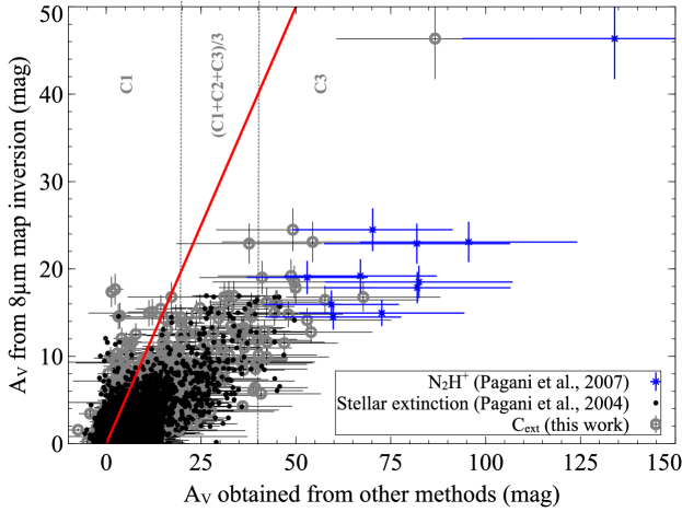
Figure 1: Comparison between A_V obtained from different methods at the 20” resolution. The A_V obtained from the 8 $\mu$m map inversion is associated to the highest peak value (I_bg,min = 0.42 MJy sr^-1). The red line shows the one-to-one relation. Gray lines and C1, C2, C3 refer to the different catalogs used to build the extinction map.

The first step in obtaining 8_ext was to subtract the stellar and background intensities from Spitzer maps, following the method of Lefèvre et al. (2014). The residual signal ($\Delta$) decreases to $-350$ kJy sr^-1($\Delta_{\mathrm{min}}$) toward the prestellar core (PSC) at 8 $\mu$m. If we suppose that the extinction is only due to absorption by the dust, as in Bacmann et al. (2000), it is directly related to $\Delta$ by $\Delta$ = I_bg ${(\mathrm{e}^{-\tau_{8}}-1)}$, where $\tau_{8}$ is the 8 $\mu$m dust opacity integrated along the line of sight, and I_bg is the background intensity value. Using nearby stars for which the stellar type is known (Whittet et al. 2013 and Fig. 5), the value of I_bg was independently estimated from the 8 $\mu$m map. Among the eight stars falling onto the 8 $\mu$m map, we kept the ones for which the $\Delta$ value is reliable (3$\sigma$ $\sim$ 60 kJy sr^-1). Since we make the approximation that the $\tau_{8}$ value from each star is locally the same as the one in its vicinity, we also eliminated the H star, saturated at 8 $\mu$m. We were left with three stars (B, D, I) with a known E(J–K)=(J-K)${}_{\mathrm{2MASS}}-$(J-K)₀. From their E(J–K), we obtained the $\tau_{8}$ values by assuming A₈/A_K conversion coefficients. We adopted the same conversion coefficients as the ones used to obtain the c1 and c2 maps, which give a range of possible values for $\tau_{8}$ (Table 1).

Table 1: Background values calculated at the vicinity of the stars. The star names and E(J–K) values refer to Whittet et al. (2013) and the (3.1) and (5.5B) notations to the dust models from Weingartner & Draine (2001).

Star	E(J–K)	$\tau_{\mathrm{8}}$	$\tau_{\mathrm{8}}$	$\Delta$	Ibg,min	Ibg,max
	mag	3.1	5.5B	kJy sr-1	MJy sr-1	MJy sr-1
B	0.62	0.067	0.15	–64 $\pm$ 6	0.42	1.08
D	0.70	0.076	0.17	–62 $\pm$ 6	0.36	0.93
I	2.49	0.27	0.60	-80 $\pm$ 8	0.16	0.37

The calculated background values are minimal (I_bg,min) for WD01(5.5B) and maximal (I_bg,max) for WD01(3.1). The compatible I_bg values between stars B and D range from 0.42 to 0.93 MJy sr^-1 (Table 1), which is comparable to the values proposed by Lefèvre et al. (2014) from a different method. Nevertheless, I_bg calculated from the I star is unreasonably low, since only I${}_{\mathrm{bg}}\geq|\Delta_{\mathrm{min}}|$ are physically meaningful. The value of I_bg,max from Star I is slightly compatible with the I_bg,min obtained for Stars B and D, but is calculated with a lower R_V value. This is not expected because Star I is more attenuated than Stars B and D, from their E(J–K) values. Given this incompatibility, we rely only on Stars B and D for the I_bg value and will revisit Star I in the discussion. From the I_bg range, we retrieve the $\tau_{8}$ maps and adopt their associated conversion coefficients to obtain the extinction maps: A₈/A_V(3.1)=0.02 for I_bg=0.93 MJy sr^-1  and A₈/A_V(5.5B)=0.045 for I_bg=0.42 MJy sr^-1.

The peak value obtained for the 8_ext map (34 or 82 mag) at 2.8″  resolution is too low when compared to the value obtained from N₂H⁺ observations (Pagani et al. 2007; Lique et al. 2015). In fact, inside a 10″ radius, the column density of N(H₂) is 1.2${}^{+0.5}_{-0.3}\times$10²³ cm^-2, which corresponds to an extinction of at least A_V = 130${}_{-32}^{+54}$ mag when assuming the Bohlin et al. (1978) conversion. Moreover, 8_ext is systematically lower than C_ext beyond 25 magnitudes of extinction (Fig. 1). The region where the 8 $\mu$m inversion fails to reproduce stellar extinction corresponds to the northern filament and its surroundings (Fig. 5). In this region, the low values given by the inversion of the 8 $\mu$m map could not explain the diminishing numbers of background stars in NIR+MIR.

Thanks to the ample number of star counts and overlapping of the techniques between A_V ranges, we have confidence in the A_V values estimated from stellar extinction. This result is confirmed by the compatibility of our C_ext map with N₂H⁺ estimates, as well as dust seen in emission at 1.2 mm (Pagani et al. 2004, Fig. 1). Considering more sophisticated methods of building C_ext would help to reduce the uncertainties (i.e., Foster et al. 2008) but would not compensate for the difference between C_ext and 8_ext (Fig. 5). Thus, the only way to explain the discrepancy between the 8_ext map and other column density estimates is by considering that the apparent extinction is weaker than the true extinction owing to an additional component. Polycyclic Aromatic Hydrocarbons (PAHs) have already been excluded in this cloud (Steinacker et al. 2010), and given the extremely cold temperatures inside the cloud, we are left with scattering as the only plausible source of compensation.

3 Modeling with scattering

If significant, the scattering contribution, I_sca, is part of the measured $\Delta$ value: $\Delta\,=\,$I${}_{\mathrm{bg}}{(\mathrm{e}^{-\tau_{8}}-1)}$ + I_sca. We estimated I_sca following several steps. First, we build a representative cloud density model based on C_ext and N₂H⁺ information. To compare the modeling with observations, we adopt a background value consistent with the extinction toward Stars B and D at 8 $\mu$m (Table 1). Then, we vary the dust properties inside the cloud density model until finding a compatible solution with the 8 $\mu$m map. Finally, we validate our solution using several tests.

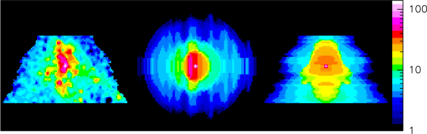
Figure 2: A_V maps of the cloud model with the common color scale in magnitudes. Left: facing the cloud; middle: from above; right: from the side.

To study the scattering contribution, it is mandatory to consider the anisotropy of the radiation field, by using a 3D radiative transfer code and take that opportunity to include a 3D cloud model (Lefèvre et al. 2014). First, we use the C_ext map, and make a rotational symmetry to obtain the 3D model. Given the velocity gradient inside the northern filament (Pagani et al. 2009) and the triangular flaring shape of the cloud, we required that the model be as elongated in depth as in width. This first approximation might not be correct, but is sufficient for our needs. A central core compatible with the N₂H⁺ density profile (Pagani et al. 2007; Lique et al. 2015) was placed at the cloud center, and densities were scaled in the third dimension to reproduce the absolute column density (Fig. 2 – left). The resolution adopted for the modeling is 20″ per cell to correctly sample the NIR extinction maps.

Assuming this cloud model, we estimated $\tau_{8}$ and its associated peak scattering intensity from I_sca = $\Delta_{\mathrm{min}}-\mathrm{I}_{\mathrm{bg}}(\mathrm{e}^{-\tau_{\mathrm{8,max}}}-1)$. The strength of the scattering component has to vary from $\sim$100 kJy sr^-1 for the lowest I_bg value to several hundred kJy sr^-1 for the highest I_bg value. With this rough estimate, we expect at least as much scattering in the 8 $\mu$m band as in the 3.6 $\mu$m band and, depending on the true background value, possibly more. Among the previous dust models tested in Lefèvre et al. (2014), only a few are able to scatter enough in the 8 $\mu$m Spitzer band. We chose to test two sets of dust models (Fig. 3): the compact spherical dust models from WD01, and the fluffy aggregates of monomers (Min et al. 2015, App. B). As a simplification, we chose a bimodal distribution with one population of small compact spherical grains (WD01, R_V = 3.1) that dominates the external regions with no scattering, and large aggegates (MIN_4.0) to progressively fill the inner region. Using the CRT radiative transfer code of Juvela & Padoan (2003), the appropriate balance between the two dust populations was constrained by the coreshine intensity ($\Delta_{3.6}$) with the I_bg value at 3.6 $\mu$m taken from Lefèvre et al. (2014).

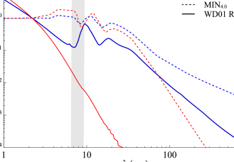
Figure 3: Dust optical properties (scattering efficiency, Q_sca, in red, total extinction efficiency, Q_ext, in blue). The WD01 (3.1) model is displayed by solid lines, and MIN fluffy aggregates with an equivalent spherical size of 4.0 $\mu$m are plotted with dotted lines. A gray area represents the 8 $\mu$m filter width. All the dust coefficients have been normalized by their value at the K_s wavelength.

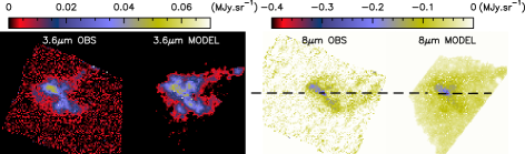
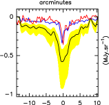
Figure 4: From left to right: 3.6 $\mu$m observations with subtracted background and stars ($\Delta_{3.6}$) compared to its modeling, and the same at 8 $\mu$m ($\Delta_{8}$). The black dashed line shows the horizontal cut through the core represented in the last panel. The red line corresponds to the profile from observations ($\Delta_{8}$), and the yellow filled shape displays modeling profiles without I_sca for I_bg values ranging from 0.42 to 0.93 MJy sr^-1. The black profile is the one example without I_sca for I_bg = 0.58 MJy sr^-1, and the blue one is the same model when including I_sca.

4 Compability of the modeling with observations

Assuming a cloud model compatible with both the NIR extinction and the N₂H⁺density, we find that the associated $\Delta$ values derived from the models are always deeper than the observed values when not considering I_sca (Fig. 4). However, when the I_sca contribution is taken into account, it is possible to find a suitable solution by including the right abundance of dust that is able to scatter at 8 $\mu$m. Given the degeneracy of the solutions and the assumptions regarding the cloud geometry, we chose to illustrate the I_sca contribution with our bimodal dust populations and focus on their relative abundances. A variation in the relative abundance of the MIN_4.0 population proportional to the density n^0.25 gives an adequate match to the horizontal cut toward the core, as well as good agreement between the observed and model $\Delta$ values at 3.6 and 8 $\mu$m (Fig. 4). The dust mass is fixed in our modeling, which does not include ices, and corresponds to grain growth by coagulation with the density. Ice coatings may promote coagulation by changing the sticking coefficient of the grains and the scattering efficiency at coreshine wavelength (Andersen et al. 2014; Lefèvre et al. 2014). However, no ice-coated dust distribution, able to produce efficient scattering at 8 $\mu$m , is publicly available presently.

Table 2: Background values derived from modeling. I_bg : calculated with $\Delta$ values from Table 1. A_V : deduced from E(J–K).

Star	$\tau_{8}^{\ast}$	$\tau_{9.7}^{\ast}$	I${}_{\mathrm{sca}}^{\ast}$	Ibg	AV
		peak	kJy sr-1	MJy sr-1	mag
B	0.16 $\pm$ 0.02	0.19 $\pm$ 0.05	41 $\pm$ 4	0.58–0.88	2.2
D	0.21 $\pm$ 0.02	0.25 $\pm$ 0.05	65 $\pm$ 7	0.56–0.81	2.5
I	0.62 $\pm$ 0.06	0.47 $\pm$ 0.09	170 $\pm$ 17	0.46–0.64	8.8

We find that even if the scattering is negligible in front of the stars compared to the stellar flux, it is not the case in their vicinity, where the I_bg value has been deduced. Taking the I_sca values in the region of the stars into account, we calculated again I_bg  (see Sect. 3) based on the $\tau_{8}^{\ast}$ values around Stars B, D, and I obtained from modeling (Table 2). We confirm that the I_bg value used for the modeling is now compatible with the three stars (Fig. 4: I_bg = 0.58 MJy sr^-1). Moreover, $\tau_{8}^{\ast}$ values are similar to the ones calculated with WD01 5.5B (Table 1). We also obtained (Table 2 and App. C) compatible values at the silicate absorption peak ($\tau_{9.7}^{\ast}$) with the ones of Whittet et al. (2013). However, grain growth by coagulation is expected to contribute to the relative decrease in $\tau_{9.7}$ with respect to the total dust opacities (Chiar et al. 2007), hence with $\tau_{8}^{\ast}$. Since grains are coagulating in L183, we expect to observe that $\tau_{9.7}$ would no longer be correlated beyond a given $\tau_{8}$ threshold, which is what we find from the modeling (App. C). This result confirms that $\tau_{9.7}$ might not be a good tracer of the total column density toward dark clouds.

5 Conclusions

From all the validation tests, we found that including a fraction of efficiently scattering dust grains (here the MIN_4.0 or any kind of aggregates with a scattering behavior similar to the red dashed line, Fig. 3) is mandatory for reproducing the 8 $\mu$m observations. Nevertheless, only a few available dust models are efficient enough to produce significant scattering up to 8 $\mu$m. The WD01 5.5B dust grains are somewhat efficient (I${}_{\mathrm{sca}}\sim$0.1 MJy sr^-1), but cannot reproduce the observations for an I_bg value greater than 0.4 MJy sr^-1. Aggregates are much more efficient at scattering the light at MIR wavelengths than compact spherical grains, and probably the only way to explain deeper $\Delta$ values observed toward other dense cores (i.e., IRAS16293, Pagani et al. in prep.). They are also compatible with grain growth by coagulation and with the expected deviation from the correlation of $\tau_{9.7}$ and $\tau_{8}$ with $\mathrm{E(J-K)}$. This is also in accord with the idea that grains remain fluffy even in the dense prestellar cores and protoplanetary disks (Mulders et al. 2013).
We demonstrated the importance of scattering up to 8 $\mu$m and the necessity of using realistic dust models. The final $\tau_{8}$ map obtained from the modeling is compatible with a filament at A_V$>$25 mag and a central density for the core of 1.8$\times$10⁶ cm^-3. Multiwavelength modeling, including NIR wavelengths, will place more constraints on the cloud shape and small grains, as discussed in Lefèvre et al. (2014). Since ices are present at relatively low extinction and can have an impact on coagulation and scattering efficiencies, smaller aggregates with ices (Köhler et al. 2015) will be investigated in a future paper. Adopting such dust models will also have consequencies on the interpretation of data in emission since aggregates are known to be better emitters (Stepnik et al. 2003). In this paper, the emissivities of the aggregates are higher by at least one order of magnitude at far-infrared wavelengths than for spherical grains (Fig. 3).

Appendix A Regions with significant scattering

The discrepancy between the 8 $\mu$m map inversion and other estimates for the visual extinction (Fig. 1) is not a simple offset that could be applied to the whole map, but it varies throughout the cloud (Figure 5). While green regions in the outer part can be interpreted as a lack of information in the 8 $\mu$m map due to the noise, other colors trace regions where the scattering cannot be neglected ($\gtrsim$ 25 mag).

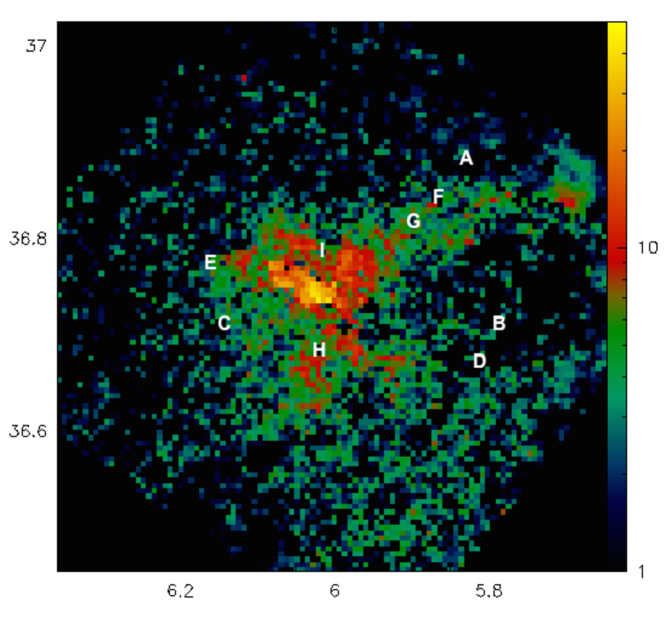
Figure 5: Difference between the visual extinction obtained via the reddening and the one via the 8 $\mu$m map inversion (in magnitudes). The letters refer to the stars studied by Whittet et al. (2013).

Appendix B The optical properties of aggregate particles

The optical properties of dust particles are very sensitive to their shape. In particular, perfect spherical particles represent a class of particles that are incompatible with observations and laboratory measurements. Therefore, we consider it very important for detailed studies of scattering properties of dust grains to use a realistic dust particle model. All details on the construction of the fluffy aggregates and their optical properties will be presented in Min et al. (2015). Below we give the basic properties needed for a proper understanding of the results presented in this paper.

The optical properties of the aggregate particles are computed using the so-called Discrete Dipole Approximation (DDA; Purcell & Pennypacker 1973; Draine & Flatau 1994). With this method one can compute the optical properties of particles with arbitrary shape and composition. Despite the confusing term ”approximation” in the name of this method, it is actually an exact method in the limit of infinite spatial resolution. We construct monomers of the aggregates by using Gaussian random field particles (Min et al. 2007). We then glue these monomers together to construct fluffy aggregates. In this way we avoid all effects of sphericity of the particles since the monomers of the aggregates are also non-spherical.

Each monomer in the aggregate is made of a single material. We randomly assign a material to each monomer using the overall composition: 75% silicate, 15% carbon, and 10% iron sulfide (by volume). This composition is roughly consistent with the solar system composition proposed by Min et al. (2011). We use the refractive index data from Dorschner et al. (1995), Preibisch et al. (1993), and Begemann et al. (1994) for the silicate (MgSiO₃), carbon, and iron-sulfide particles, respectively.

Using the DDA code ADDA (Yurkin & Hoekstra 2011), we compute the absorption, scattering, and extinction cross sections, as well as the full scattering matrix elements at wavelengths from the visible up to millimeter wavelengths for aggregates composed of 1 to 8000 monomers (corresponding to volume equivalent radii from 0.2 to 4.0$\,\mu$m).

Appendix C

To compare the $\tau_{9.7}$ values measured at the silicate absorption peak by Whittet et al. (2013) with the one from the modeling, $\tau_{9.7}^{\ast}$, we subtracted the continuum opacity from the total dust opacity at 9.7 $\mu$m. In order to verify the conversion between $\tau_{8}$ and $\tau_{9.7}$, we made a plot of the values cell by cell (Fig. 6).

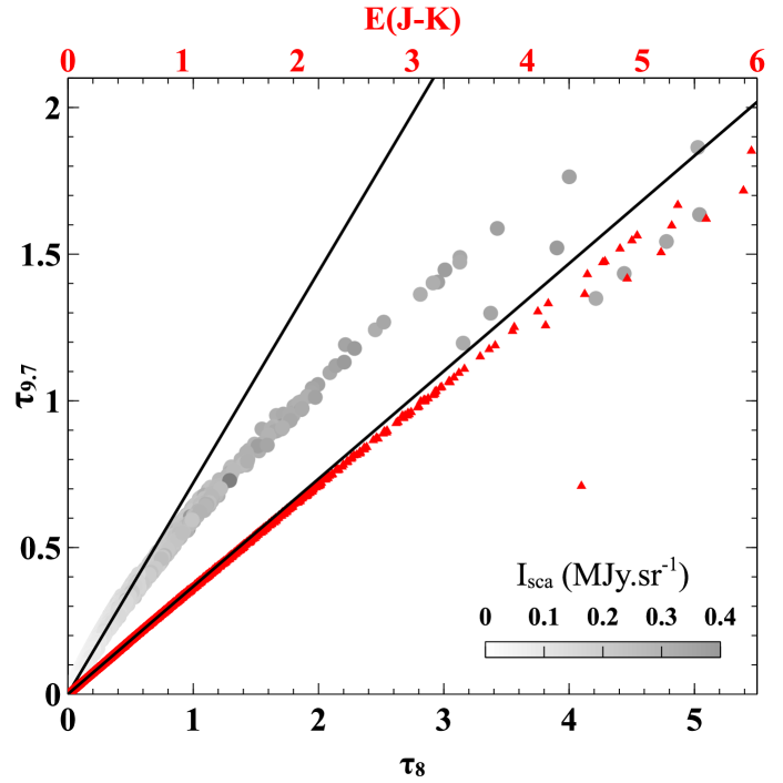
Figure 6: The 9.7 $\mu$m silicate absorption line opacities as a function of $\tau_{8}$ (gray circles). The color of the circles is related to the I_sca strength. The 9.7 $\mu$m silicate absorption line opacities as a function of E(J–K) is represented by red triangles. All the values are obtained from the modeling and black lines correspond to the correlation obtained from diffuse interstellar lines of sight (Whittet 2003).

For $\tau_{8}$ lower than 0.5, both are correlated by the relation $\tau_{9.7}$/$\tau_{8}$ $\sim$ 0.72 (red line Fig. 6) but above this threshold, the $\tau_{9.7}$ values decrease more rapidly than the correlation law. The behavior of $\tau_{9.7}$ with $\tau_{8}$ is also likely to be part of the explanation of the effect observed between $\tau_{9.7}$ and E(J–K) by Chiar et al. (2007) and by Whittet et al. (2013, towards L183). Indeed, beyond a limit of $\mathrm{E(J-K)}=2\,\mathrm{mag}$, the measured optical depth of the 9.7 $\mu$m silicate absorption feature ($\tau_{9.7}$) also decreases with respect to E(J–K) measured along diffuse interstellar lines of sight. Since $\tau_{9.7}$ measures the silicate absorption along the line of sight and not the continuum opacity from other dust species, it may not be representative of the total dust opacity toward dark clouds. Moreover, if the line of sight opacity is dominated by small silicate grains, the $\tau_{9.7}$ is expected to be less than proportional to $\tau_{8}$ with coagulation. We detect this effect from our modeling (Fig. 6) associated to an increase in I_sca that traces the coagulation. Since J and K bands are very sensitive to the cloud model (Lefèvre et al. 2014), the $\tau_{9.7}$ function of E(J–K), plotted in Fig. 6, must be considered as a simple trend at this stage.

Appendix D Institutional and technical acknowledgements

This research has made use of observations from the Spitzer Space Telescope and data from the NASA/IPAC Infrared Science Archive, which are operated by the Jet Propulsion Laboratory (JPL) and the California Institute of Technology under contract with NASA. It makes use of data products from the Wide-field Infrared Survey Explorer, which is a joint project of the University of California, Los Angeles, and the Jet Propulsion Laboratory/California Institute of Technology, funded by the National Aeronautics and Space Administration. It makes use of data products from the Two Micron All Sky Survey, which is a joint project of the University of Massachusetts and the Infrared Processing and Analysis Center/California Institute of Technology, funded by the National Aeronautics and Space Administration and the National Science Foundation. Our VISTA data are based on observations made with ESO Telescopes at the Paranal Observatory under program ID 091.C-0795. We thank L. Cambrésy and M. Juvela for providing their code to deduce NIR extinction, and M.J. for CRT. We thank P. Hudelot and N. Bouflous for the TERAPIX data treatment of our VISTA data.