From $t$-Closeness to Differential Privacy and Vice Versa in Data Anonymization

Abstract

$k$-Anonymity and $\varepsilon$-differential privacy are two mainstream privacy models, the former introduced to anonymize data sets and the latter to limit the knowledge gain that results from including one individual in the data set. Whereas basic $k$-anonymity only protects against identity disclosure, $t$-closeness was presented as an extension of $k$-anonymity that also protects against attribute disclosure. We show here that, if not quite equivalent, $t$-closeness and $\varepsilon$-differential privacy are strongly related to one another when it comes to anonymizing data sets. Specifically, $k$-anonymity for the quasi-identifiers combined with $\varepsilon$-differential privacy for the confidential attributes yields stochastic $t$-closeness (an extension of $t$-closeness), with $t$ a function of $k$ and $\varepsilon$. Conversely, $t$-closeness can yield $\varepsilon$-differential privacy when $t=\exp(\varepsilon/2)$ and the assumptions made by $t$-closeness about the prior and posterior views of the data hold.

1 Introduction

$k$-Anonymity and $\varepsilon$-differential privacy are two mainstream privacy models originated within the computer science community. Their approaches towards disclosure limitation are quite different: $k$-anonymity is a model for releases of microdata (i.e. individual records) that seeks to prevent record re-identification by hiding each original record within a group of $k$ indistinguishable anonymized records, while $\varepsilon$-differential privacy seeks to limit the knowledge gain between data sets that differ in one individual. Both models are often presented as antagonistic: $\varepsilon$-differential privacy supporters view $k$-anonymity as an old-fashioned privacy notion that offers only poor disclosure limitation guarantees (they argue that generating a a "noisy table" that safely provides accurate answers to arbitrary queries is not feasible [11]), while $\varepsilon$-differential privacy detractors criticize the limited utility of $\varepsilon$-differentially private outputs [24, 2].

In this paper we show that $t$-closeness (one of the extensions of $k$-anonymity) and $\varepsilon$-differential privacy turn out to be strongly related when it comes to anonymizing data sets. Specifically, $k$-anonymizing the quasi-identifiers of a data set and ensuring $\varepsilon$-differential privacy for the confidential attributes yields stochastic $t$-closeness (which in turn is an extension of $t$-closeness), with $t$ a function of $\varepsilon$ and of the size of the $k$-anonymity equivalence classes. Attaining standard $t$-closeness from $\varepsilon$-differential privacy is unfeasible because, being $\varepsilon$-differential privacy a stochastic mechanism, it is not possible to meet the requirements that $t$-closeness puts on the empirical distribution of the confidential attributes. To circumvent this issue, we introduce stochastic $t$-closeness, which is defined on the theoretical distribution of the confidential attribute that results from the masking procedure (rather than on a specific realization of it). Conversely, $t$-closeness can yield guarantees similar to $\varepsilon$-differential privacy for the confidential attribute. Attaining exact $\varepsilon$-differential privacy from $t$-closeness is unfeasible because, for instance, $t$-closeness fails to provide any protection if we assume that all the records except one are known by the intruder. However, if the assumptions made by $t$-closeness about the prior and posterior views of the data by the intruder hold, then the protection we get from $t$-closeness is equivalent to that of $\varepsilon$-differential privacy.

Section 2 contains background on $k$-anonymity, $t$-closeness and $\varepsilon$-differential privacy. Section 3 introduces the concept of stochastic $t$-closeness. Section 4 shows that combining $k$-anonymity and differential privacy as sketched above yields (stochastic) $t$-closeness. Section 5 shows that, under the assumptions made by $t$-closeness about the prior and posterior views of the data, $t$-closeness provides differential privacy-like privacy guarantees for the confidential attributes. A construction to attain $t$-closeness that relies on bucketization is presented in Section 6. Section 7 reviews related work. Conclusions and future research issues are summarized in Section 8.

The material in Section 6 was presented in the conference paper [28]. The rest of sections in this paper are new.

2 Background

2.1 $k$-Anonymity

Assume a data set $X$ from which direct identifiers have been suppressed, but which contains so-called quasi-identifier attributes, that is, attributes (e.g. age, gender, nationality, etc.) which can be used by an intruder to link records in $X$ with records in some external database containing direct identifiers. The intruder’s goal is to determine the identity of the individuals to whom the values of confidential attributes (e.g. health condition, salary, etc.) in records in $X$ correspond (identity disclosure). See [17] for further details on disclosure attacks.

A data set $X$ is said to satisfy $k$-anonymity [27, 26] if each combination of values of the quasi-identifier attributes in it is shared by at least $k$ records. We use the term equivalence class to refer to a maximal set of records that are indistinguishable with respect to the quasi-identifiers. $k$-Anonymity protects against identity disclosure: given an anonymized record in $X$, an intruder cannot determine the identity of the individual to whom the record (and hence the confidential attribute values in it) corresponds. The reason is that there are at least $k$ records in $X$ sharing any combination of quasi-identifier attribute values.

The most usual computational procedure to attain $k$-anonymity is generalization of the quasi-identifier attributes [26], but an alternative approach is based on microaggregation of the quasi-identifier attributes [7].

2.2 $t$-Closeness

While $k$-anonymity protects against identity disclosure, as mentioned above, it does not protect in general against attribute disclosure, that is, disclosure of the value of a confidential attribute corresponding to an external identified individual. Let us assume a target individual $T$ for whom the intruder knows the identity and the values of the quasi-identifier attributes. Let $G_{T}$ be a group of at least $k$ anonymized records sharing a combination of quasi-identifier attribute values that is the only one compatible with $T$’s quasi-identifier attribute values. Then the intruder knows that the anonymized record corresponding to $T$ belongs to $G_{T}$. Now, if the values for one (or several) confidential attribute(s) in all records of $G_{T}$ are the same, the intruder learns the values of that (those) attribute(s) for the target individual $T$.

The property of $l$-diversity [23] has been proposed as an extension of $k$-anonymity which tries to address the attribute disclosure problem. A data set is said to satisfy $l$-diversity if, for each equivalence class, there are at least $l$ “well-represented” values for each confidential attribute. Achieving $l$-diversity in general implies more distortion than just achieving $k$-anonymity. Yet, $l$-diversity may fail to protect against attribute disclosure if the $l$ values of a confidential attribute are very similar or are strongly skewed. $p$-Sensitive $k$-anonymity [30] is a property similar to $l$-diversity, which shares similar shortcomings. See [8] for a summary of criticisms to $l$-diversity and $p$-sensitive $k$-anonymity.

$t$-Closeness [20] is another extension of $k$-anonymity which also tries to solve the attribute disclosure problem.

Definition 1

An equivalence class is said to satisfy $t$-closeness if the distance between the distribution of a sensitive attribute in this class and the distribution of the attribute in the whole table is no more than a threshold $t$. A table is said to satisfy $t$-closeness if all its equivalence classes satisfy $t$-closeness.

$t$-Closeness clearly solves the attribute disclosure vulnerability, although the original paper [20] did not propose a computational procedure to achieve this property and did not mention the large utility loss that achieving it is likely to inflict on the original data.

2.3 $\varepsilon$-Differential privacy

Differential privacy was proposed by [9] as a relative privacy model that limits the knowledge gain between data sets that differ in one individual.

Definition 2

A randomized function $\kappa$ gives $\varepsilon$-differential privacy if, for all data sets $D_{1}$, $D_{2}$ such that one can be obtained from the other by modifying a single record, and all $S\subset Range(\kappa)$

$$\Pr(\kappa(D_{1})\in S)\leq\exp(\varepsilon)\times\Pr(\kappa(D_{2})\in S)$$ (1)

Originally the focus was on the interactive setting; that is, to protect the outcomes of queries to a database. The assumption is that an anonymization mechanism sits between the user submitting queries and the database answering them. The computational mechanism to attain $\varepsilon$-differential privacy is often called $\varepsilon$-differentially private sanitizer. A usual sanitization approach is noise addition: given a query $f$, the real value $f(D)$ is computed, and a random noise, say $Y(D)$, is added to mask $f(D)$, that is, a randomized response $\kappa(D)=f(D)+Y(D)$ is returned. To generate $Y(D)$, a common choice is to use a Laplace distribution with zero mean and $\Delta(X)/\varepsilon$ scale parameter, where:

• $\varepsilon$ is the differential privacy parameter;

• $\Delta(f)$ is the $L_{1}$-sensitivity of $f$, that is, the maximum variation of the query function between neighbor data sets, i.e., sets differing in at most one record.

Differential privacy was also developed for the non-interactive setting in [3, 14, 16, 4]. Even though a non-interactive data release can be used to answer an arbitrarily large number of queries, in all these proposals this feature is obtained at the cost of preserving utility only for restricted classes of queries (typically count queries). This contrasts with the general-purpose utility-preserving data release offered by the $k$-anonymity model.

3 Stochastic $t$-closeness

The fact that differential privacy is stochastic, while $t$-closeness is deterministic, makes it impossible to guarantee that a differentially private data set will satisfy $t$-closeness. To bridge this gap, we introduce the concept of stochastic $t$-closeness.

Let $X$ be a data set with quasi-identifier attributes collectively denoted by $QI$ and confidential attributes $C_{1},C_{2},\cdots,C_{n}$. Let $N$ be the number of records of $X$.

To attain $t$-closeness we need to partition $X$ into equivalence classes such that the (empirical) distribution of the confidential attributes over the entire $X$ is close to the (empirical) distribution of the confidential attributes within each of the equivalence classes: the distance between the former distribution and each of the latter distributions must be less than a threshold value $t$. If $c_{1},c_{2},\cdots,c_{N}$ are the values of a confidential attribute in $X$, and $c_{1},c_{2},\cdots,c_{|E|}$ are the values of that attribute within equivalence class $E$, the respective empirical distributions $\Pr(\cdot)$ and $\Pr_{E}(\cdot)$ can be computed as

$${\Pr}(B)=\frac{1}{N}\sum_{i=1,2,\cdots,N}{\Pr}_{\mathbbm{1}_{c_{i}}}(B)$$

and

$${\Pr}_{E}(B)=\frac{1}{|E|}\sum_{i=1,2,\cdots,|E|}{\Pr}_{\mathbbm{1}_{c_{i}}}(B)$$

where $B$ is any subset of values of the attribute, and $P_{\mathbbm{1}_{c_{i}}}(B)=1$ if and only if $c_{i}\in B$.

The standard practice to generate a $t$-close data set $X^{\prime}$ out of $X$ favors preserving the values of the confidential attributes within each of the equivalence classes. Probably the reason has to do with $t$-closeness being an extension of $k$-anonymity. $k$-Anonymity is not concerned with the values of the confidential attributes and, thus, attaining $k$-anonymity does not require any operation on them. $t$-Closeness was initially attained by incorporating its constraints into $k$-anonymous data set generation algorithms; in this way, the values of the confidential attributes within each equivalence class were kept unmodified. In [20] and [21], the Incognito [19] and the Mondrian [18] algorithms that were designed for $k$-anonymity are adapted for $t$-closeness. Modification of the confidential values was considered in [25]. Let $f$ be a function that masks the confidential attributes to bring the empirical distribution of the modified equivalence classes closer to the empirical distribution of the modified whole data set. Using the previous notations, the modified empirical distributions are computed as

$${\Pr}(B)=\frac{1}{N}\sum_{i=1,2,\cdots,N}{\Pr}_{\mathbbm{1}_{f(c_{i})}}(B)$$

and

$${\Pr}_{E}(B)=\frac{1}{|E|}\sum_{i=1,2,\cdots,|E|}{\Pr}_{\mathbbm{1}_{f(c_{i})}}(B).$$

The previous masking function $f$ is deterministic, but dealing with stochastic masking functions would be interesting. Let $Z$ be a stochastic function. Attaining $t$-closeness is not possible for $Z$, as the actual values depend on each specific realization of $Z$. However, there is a natural extension of the concept of $t$-closeness that deals smoothly with stochastic functions. Basically, we have to stop working with empirical distributions, and use the distributions determined by $Z$ instead. In terms of the formulas, we need to change $\mathbbm{1}_{f(\cdot)}$ by $Z(\cdot)$.

Definition 3

Let $X^{\prime}$ be a data set obtained from $X$ by applying a stochastic function $Z$ to its confidential attributes. We say that $X^{\prime}$ satisfies stochastic $t$-closeness if, for each equivalence class $E$, the distance between

$${\Pr}(B)=\frac{1}{N}\sum_{i=1,2,\cdots,N}{\Pr}_{Z(c_{i})}(B)$$

and

$${\Pr}_{E}(B)=\frac{1}{|E|}\sum_{i=1,2,\cdots,|E|}{\Pr}_{Z(c_{i})}(B)$$

is less than a threshold $t$.

Although a deeper analysis of stochastic $t$-closeness might be interesting, our aim here is to relate it to differential privacy and the above definition will suffice to this aim.

4 From differential privacy to (stochastic) $t$-closeness

This section develops one of the main results in this paper: the implication between $\varepsilon$-differential privacy and stochastic $t$-closeness. Before going into that result, we need to deal with an important aspect of $t$-closeness: the distance between the probability distributions used.

Stochastic $t$-closeness, just as $t$-closeness, is about making the distance between the data set-level and the equivalence class-level distribution of the confidential attribute less than a threshold value $t$ for any equivalence class. When $t$-closeness was introduced, the Earth Mover’s distance (EMD) was proposed [20]. The EMD measures the minimal amount of work required to transform one distribution into another by moving probability mass between each other.

The specific distance used can actually be viewed as an additional parameter of $t$-closeness and it has a significant impact on the kind of privacy guarantees offered. As we aim to show that differential privacy for the confidential attributes leads to stochastic $t$-closeness, we take a distance function that is more suited to differential privacy.

Definition 4

Given two random distributions $\mathcal{D}_{1}$ and $\mathcal{D}_{2}$, we define the distance between $\mathcal{D}_{1}$ and $\mathcal{D}_{2}$ as:

$$d(\mathcal{D}_{1},\mathcal{D}_{2})=\max_{S}\left\{\frac{\Pr_{\mathcal{D}_{1}}(S)}{\Pr_{\mathcal{D}_{2}}(S)},\frac{\Pr_{\mathcal{D}_{2}}(S)}{\Pr_{\mathcal{D}_{1}}(S)}\right\}$$

where $S$ is an arbitrary (measurable) set, and we take the quotients of probabilities to be zero, if both $\Pr_{\mathcal{D}_{1}}(S)$ and $\Pr_{\mathcal{D}_{2}}(S)$ are zero, and to be infinity if only the denominator is zero.

We are ready to move to the main result of the section: the implication between differential privacy and $t$-closeness.

Proposition 1

Let $X$ be an original data set and $X^{\prime}$ be a corresponding anonymized data set such that the projection of $X$ on the confidential attributes is $\varepsilon$-differentially private. Then $X$ satisfies stochastic $t$-closeness with

$$t=\max_{E}\frac{|E|}{N}\left(1+\frac{N-|E|-1}{|E|}\exp(\varepsilon)\right)$$

where $E$ is an equivalence class.

Proof. Let $E$ be an equivalence class of $X$ and let $c_{1},c_{2},\cdots,c_{|E|}$ be the values of the projection of $X$ on the confidential attributes. For $t$-closeness to hold, it must be $\Pr_{E}(B)\leq t\times\Pr(B)$ and $\Pr(B)\leq t\times\Pr_{E}(B)$, for any $B$.

We start by deriving an inequality that will later be used. If $Z$ satisfies $\varepsilon$-differential privacy, we have $\exp(-\varepsilon)\times\Pr_{Z(c_{j})}(B)\leq\Pr_{Z(c_{i})}(B)\leq\exp(\varepsilon)\times\Pr_{Z(c_{j})}(B)$, for all $i$ and $j$. In particular, we have

$$\frac{\exp(-\varepsilon)}{|E|}\sum_{j=1,2,\cdots,|E|}{\Pr}_{Z(c_{j})}(B)\leq{\Pr}_{Z(c_{i})}(B)$$

$$\leq\frac{\exp(\varepsilon)}{|E|}\sum_{j=1,2,\cdots,|E|}{\Pr}_{Z(c_{j})}(B).$$

Let $d=\sum_{i=1,2,\cdots,|E|}{\Pr}_{Z(c_{i})}(B)$. The previous equation becomes $\frac{1}{|E|}\exp(-\varepsilon)d\leq{\Pr}_{Z}(c_{i})\leq\frac{1}{|E|}\exp(\varepsilon)d$. By taking the sum for $i$ in $|E|+1,|E|+2,\cdots,N$, we have

$$\frac{N-|E|}{|E|}\exp(-\varepsilon)d\leq\sum_{i=|E|+1,|E|+2,\cdots,N}{\Pr}_{Z(c_{i})}(B);$$ (2)

$$\sum_{i=|E|+1,|E|+2,\cdots,N}{\Pr}_{Z(c_{i})}(B)\leq\frac{N-|E|}{|E|}\exp(\varepsilon)d.$$ (3)

Now we turn to the $t$-closeness requirements. We start with ${\Pr}_{E}(B)\leq t\times{\Pr}(B)$. This inequality can be rewritten as

$$\frac{1}{|E|}\sum_{i=1,2,\cdots,|E|}{\Pr}_{Z(c_{i})}(B)\leq t\times\frac{1}{N}\sum_{i=1,2,\cdots,N}{\Pr}_{Z(c_{i})}(B).$$

In terms of $d$ it becomes

$$\frac{1}{|E|}\times d\leq t\frac{1}{N}\left(d+\sum_{i=|E|+1,|E|+2,\cdots,N}{\Pr}_{Z(c_{i})}(B)\right).$$

By Inequality (2) the following inequality implies the previous one

$$\frac{1}{|E|}\times d\leq t\frac{1}{N}\left(d+\frac{N-|E|}{|E|}\exp(-\varepsilon)d\right)$$

By operating on the previous inequality we get

$$t\geq\frac{N}{|E|}\left(1+\frac{N-|E|}{|E|}\exp(-\varepsilon)\right)^{-1}.$$

By following a similar process with inequality $P(B)\leq t\times P_{E}(B)$ we conclude

$$t\geq\frac{|E|}{N}\left(1+\frac{N-|E|}{|E|}\exp(\varepsilon)\right).$$

The conclusion is that if $Z$ satisfies $\varepsilon$-differential privacy, then we get $t$-closeness on $X^{\prime}$ for

$$t=\max_{E}\{\frac{N}{|E|}\left(1+\frac{N-|E|}{|E|}\exp(-\varepsilon)\right)^{-1},$$

$$\frac{|E|}{N}\left(1+\frac{N-|E|}{|E|}\exp(\varepsilon)\right)\}.$$

It can be seen that the second term is always greater than the first one, which leads to

$$t=\max_{E}\frac{|E|}{N}\left(1+\frac{N-|E|-1}{|E|}\exp(\varepsilon)\right).$$

$\Box$

There are two approaches to enforce $t$-closeness for a data set that contains multiple confidential attributes: (i) take the confidential attributes together as a single confidential attribute and seek $t$-closeness for it using the joint distribution, and (ii) deal with each confidential attribute separately, that is, seek $t$-closeness independently for each confidential attribute. The first approach is stronger in terms of privacy guarantees, and it is the one we have used in the previous proposition. If instead of having $\varepsilon$-differential privacy for the projection of the data set on the confidential attributes we had $\varepsilon$-differential privacy for each individual attribute, then the second approach would be more suitable.

Proposition 2 shows that $\varepsilon$-differential privacy for the confidential attributes implies (stochastic) $t$-closeness for a $t$ that depends on the number of records, the cardinality of the equivalence classes and $\varepsilon$. The proposition shows that $\varepsilon$-differential privacy is stronger than (stochastic) $t$-closeness as a privacy model. From a more practical point of view, Proposition 2 can be seen as a possible approach to generate a $t$-close data set. The confidential attribute of such a data set has not only the privacy guarantees provided by $t$-closeness but also the ones given by $\varepsilon$-differential privacy.

5 $\varepsilon$-Differential privacy through $t$-closeness

In this section we show that if the conditions under which $t$-closeness provides its privacy guarantee hold for a data set, then we have differential privacy on the projection over the confidential attributes.

The quasi-identifier attributes are excluded from our discussion. The reason is that $t$-closeness offers no additional protection to the quasi-identifiers beyond what $k$-anonymity does. For example, we may learn that an individual is not in the data set if there is no equivalence class in the released $t$-close data whose quasi-identifier values are compatible with the individual’s.

The main requirement for the implication between $t$-closeness and differential privacy relates to the satisfaction of the $t$-closeness requirements about the prior and posterior knowledge of an observer. $t$-Closeness assumes that the distribution of the confidential data is public information (this is the prior view of observers about the confidential data) and limits the knowledge gain between the prior and posterior view (the distribution of the confidential data within the equivalence classes) by limiting the distance between both distributions.

Similarly to Section 4, to make $t$-closeness closer in meaning to differential privacy, we use the distance proposed in Definition 4. If the distributions $\mathcal{D}_{1}$ and $\mathcal{D}_{2}$ of Definition 4 are discrete (as is the case for the empirical distribution of a confidential attribute in a microdata set), computing the distance between them is simpler: taking the maximum over the possible individual values suffices.

Proposition 2

If distributions $\mathcal{D}_{1}$ and $\mathcal{D}_{2}$ take values in a discrete set $\{x_{1},x_{2}$ $\cdots,$ $x_{N}\}$, then the distance $d(\mathcal{D}_{1},\mathcal{D}_{2})$ can be computed as

$$d(\mathcal{D}_{1},\mathcal{D}_{2})=\max_{i=1,2,\cdots,N}\left\{\frac{\Pr_{\mathcal{D}_{1}}(x_{i})}{\Pr_{\mathcal{D}_{2}}(x_{i})},\frac{\Pr_{\mathcal{D}_{2}}(x_{i})}{\Pr_{\mathcal{D}_{1}}(x_{i})}\right\}.$$ (4)

Suppose that $t$-closeness holds; that is, the data set $X^{\prime}$ consists of several equivalence classes selected in such a way that the multiplicative distance proposed in Definition 4 between the distribution of the confidential attribute over the whole data set and the distribution within each of the equivalence classes is less than $t$. We will show that, if the assumption on the prior and posterior views of the data made by $t$-closeness holds, then $\exp(\varepsilon/2)$-closeness implies $\varepsilon$-differential privacy. A microdata release can be viewed as the collected answers to a set of queries, where each query requests the attribute values associated to a different individual. As the queries relate to different individuals, checking that differential privacy holds for each individual query suffices, by parallel composition, to check that it holds for entire data set. Let $I$ be a specific individual in the data set. For differential privacy to hold for the query associated to individual $I$, including $I$’s data in the data set vs not including them must modify the probability of the output by a factor not greater than $\exp(\varepsilon)$, where $\varepsilon$ is differential privacy parameter.

Proposition 3

Let $k_{I}(D)$ be the function that returns the view on $I$’s confidential data given $D$. If the assumptions required for $t$-closeness to provide a strong privacy guarantee hold, then $\exp(\varepsilon/2)$-closeness on $D$ implies $\varepsilon$-differential privacy of $k_{I}$. In other words, if we restrict the domain of $k_{I}$ to $\exp(\varepsilon/2)$-close data sets, then we have $\varepsilon$-differential privacy for $k_{I}$.

Proof. Let $D_{1}$ and $D_{2}$ be two data sets satisfying $\exp(\varepsilon/2)$-closeness for the combination of all confidential attributes. For $\varepsilon$-differential privacy to hold, we need $\Pr(k_{I}(D_{1})\in S)\leq\exp(\varepsilon)\times\Pr(k_{I}(D_{2})\in S)$. We consider four different cases: (i) $I\notin D_{1}$ and $I\notin D_{2}$, (ii) $I\notin D_{1}$ and $I\in D_{2}$, (iii) $I\in D_{1}$ and $I\notin D_{2}$, and (iv) $I\in D_{1}$ and $I\in D_{2}$.

In case (i), the posterior view does not provide information about $I$ beyond the one in the prior view: we have $k_{I}(D_{1})=k_{I}(D_{2})$. Hence, $\varepsilon$-differential privacy is satisfied.

Cases (ii) and (iii) are symmetric. We focus on case (ii). Given the assumptions, we have that $k_{I}(D_{1})$ has the distribution of the confidential attribute on the whole table, while $k_{I}(D_{2})$ has the distribution of the confidential attribute of the equivalence class that contains $I$. Because of $\exp(\varepsilon/2)$-closeness, the distributions of $k_{I}(D_{1})$ and $k_{I}(D_{2})$ differ by a factor not greater than $\exp(\varepsilon/2)$ and, therefore, satisfy $\varepsilon$-differential privacy.

Case (iv) is a composition of the previous case for $k_{I}(D_{1})$ and $k_{I}(D_{2})$. Both $k_{I}(D_{1})$ and $k_{I}(D_{2})$ differ from the distribution of the confidential attribute on the whole table by a factor of $\exp(\varepsilon/2)$. Thus, they differ from each other by a factor not greater than $\exp(\varepsilon)$, as we wanted. $\Box$

Parallel to what we did in Section 4, the previous proposition deals with all confidential attributes at once. That is, we assume that $t$-closeness holds for the combination of all the confidential attributes and we see that we get differential privacy for the same combination of attributes. If $t$-closeness is satisfied only for a specific confidential attribute (or subset of confidential attributes), then we get differential privacy for that attribute (or subset of confidential attributes).

Proposition 3 shows that, if the assumptions of $t$-closeness about the prior and posterior views of the intruder are satisfied, then the level of disclosure risk limitation provided by $t$-closeness is as good as the one of $\varepsilon$-differential privacy. Of course, differential privacy is independent of the prior knowledge, so Proposition 3 does not apply in general. However, when it applies, it provides an effective way of generating an $\varepsilon$-differentially private data set.

6 A bucketization construction to attain $t$-closeness

We want to reach $t$-closeness using the distance of Definition 4. A problem we face is that $t$-closeness is not attainable if there are confidential attribute values with multiplicity less than the number of equivalence classes. The reason is that, when an equivalence class lacks one of the values of the confidential attribute, the distance between the equivalence class-level distribution and the data set-level distribution is infinity (according to Definition 4). To circumvent this issue, instead of working with the empirical distribution of the confidential attribute, we work with a bucketized version of it, where points are clustered into a set of buckets $B_{1},B_{2},\cdots,B_{n}$.

Before going into the details, we give an overview of the steps required to attain $t$-closeness. Figure 1 shows two sets of data. At the top there are the original values of the confidential attribute. According to the previous discussion, $t$-closeness (for a finite $t$) is not feasible for it. At the bottom, there is a version of the confidential attribute where data have been clustered in buckets $B_{1}$, $B_{2}$ and $B_{3}$ that contain four points each. The granularity reduction of the data makes it feasible to attain $t$-closeness for a finite $t$.

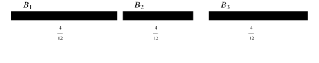
Figure 1: Top, original confidential attribute values. Bottom, bucketized confidential attribute values.

For instance, Figure 2 shows a partition of the data set in equivalence classes that satisfies $1.5$-closeness, according to the previously defined distance. The empirical distribution of the original data assigns probability $1/3$ to each of the buckets $B_{1}$, $B_{2}$ and $B_{3}$; hence, the bucket-level distribution $\mathcal{D}$ of the confidential attribute in the original data set is $\Pr(B_{1})=\Pr(B_{2})=\Pr(B_{3})=1/3$. Each of the equivalence classes in the partition ($E_{1}$, $E_{2}$, $E_{3}$) takes either one or two points from each bucket. Thus, the bucket-level empirical distribution $\mathcal{D}(E_{1})$ of the confidential attribute for equivalence class $E_{1}$ is $\Pr(B_{1})=1/2$ and $\Pr(B_{2})=\Pr(B_{3})=1/4$; for equivalence class $E_{2}$, the distribution, denoted by $\mathcal{D}(E_{2})$, is $\Pr(B_{1})=\Pr(B_{3})=1/4$ and $\Pr(B_{2})=1/2$; for equivalence class $E_{3}$, the distribution, denoted by $\mathcal{D}(E_{3})$, is $\Pr(B_{1})=\Pr(B_{2})=1/4$ and $\Pr(B_{3})=1/2$. By using Equation (4) to measure the distance between $\mathcal{D}$ and $\mathcal{D}(E_{i})$, for all $i$, we conclude that the generated partition satisfies $1.5$-closeness. In Figure 2 we have depicted both the original set of values of the confidential attribute and the generated buckets.

	original data
	equivalence class $E_{1}$
	equivalence class $E_{2}$
	equivalence class $E_{3}$

Figure 2: Sample partition that satisfies $1.5$-closeness

The rest of the section focuses on determining the conditions that the bucketization and the partition in equivalence classes must satisfy to maximize data utility. To fix notations, we assume a data set $X$ of size $N$. The granularity of the confidential attribute is reduced by considering $b$ buckets $B_{1},B_{2},\cdots,B_{b}$, each of them containing $b_{i}$ original values (that is, each of them having probability $b_{i}/N$). The partition in equivalence classes consists of $e$ equivalence classes $E_{1},E_{2},\cdots,E_{e}$, each of them containing $e_{i}$ (bucketized) records. Let $k$ be the minimum among the $e_{i}$’s.

The necessary condition, discussed at the beginning of the section, for $t$-closeness to be attainable can be reformulated according to the stated notation as $b_{i}\geq e$ for all $i$.

6.1 Optimal bucketization

The selected bucketization of the confidential attribute has a large impact on data utility. To minimize the damage to data utility we should generate buckets that are as homogeneous as possible. In general, if a distance function is used to measure the similarity of the values of the confidential attribute, a clustering algorithm can be used to generate homogeneous buckets. The size of the buckets is a parameter that can have a large impact on bucket homogeneity: the smaller the buckets, the more homogeneous they can be. However, taking too small buckets may defeat the purpose of the bucketization, that is, reducing the granularity of the confidential attribute so that $t$-closeness is attainable. In this section we seek to determine the optimal bucket size.

Figure 3 illustrates two probability distributions: the uniform distribution represents the global distribution of the confidential attribute (over the whole data set), and the other distribution corresponds to the confidential attribute restricted to an equivalence class $E_{i}$. These two distributions satisfy $2$-closeness with the distance of Definition 4: the density of the restriction to $E_{i}$ is $1/2$ for the entire range of values of the confidential attribute, except for a subrange where it is 2.

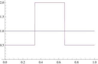
Figure 3: Probability distributions satisfying $2$-closeness with the distance of Definition 4

When bucketizing the distributions in Figure 3, the subrange with density 2 should exactly correspond to a bucket or a union of buckets, in order to maximize the utility of the resulting data. This is illustrated in Figure 4, whose top row shows bucketized versions of the distributions of Figure 3 using three buckets: top left graph, bucketized version of the global distribution; top right graph, bucketized version of the restriction to $P_{i}$. Note that, for each of the buckets, the global probability and the probability restricted to $E_{i}$ differ by a multiplicative factor of two; that is, we attain $2$-closeness with equality for each of the buckets. The bottom row of Figure 4 shows the bucketized versions of the distributions in Figure 3 using two buckets. It can be seen that, with the two proposed buckets, both bucketized distributions are identical; that is, we get $1$-closeness, which is stronger than the intended $2$-closeness, but comes at the cost of data utility loss. Therefore, the number and hence the probability mass of the optimal buckets is dependent on the level of $t$-closeness that we want.

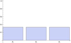
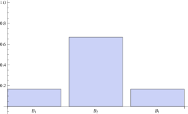
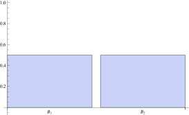
Figure 4: Bucketized distributions of the confidential attribute for the whole data (left) and for an equivalence class $E_{i}$ (right). Three buckets are considered in the top distributions, and two in the bottom ones.

According to the previous example, if the privacy requirement is $t$-closeness, for a certain $t$, it seems reasonable to use up the allowed distance $t$ between the global distribution of the confidential attribute and the restriction of that distribution within each equivalence class. Using up the allowed distance between the confidential attribute distributions enables forming equivalence classes that are more homogeneous, and hence decreases information loss.

Let us now put together what we said about the homogeneity and size of the buckets, and about the equivalence classes that emphasize a specific bucket (the probability distribution of the restriction to each equivalence class must differ from the global distribution by a factor of $t$ for a specific bucket, and by a factor of $1/t$ for the rest of buckets). The conclusion is that we should set off for the maximum number of buckets (thus, for buckets that are as small as possible) but with the constraint that equivalence classes should be able to emphasize a specific bucket. This is formulated as

$$t\times b_{i}/N+\frac{1}{t}\times(1-b_{i}/N)=1$$

for all $i$. The result is $b_{i}=N/(t+1)$ for all $i$. That is, the optimal bucketization consists of $t+1$ buckets of size $N/(t+1)$. Notice that the optimal bucketization is only attainable if $t+1$ divides $N$; otherwise we should select the closest feasible bucketization.

6.2 $t$-Closeness construction

Consider the original data set $X=\{(qi_{i},c_{i})|i=1,2,\cdots,N\}$, where $qi_{i}$ refers to the quasi-identifier attributes, and $c_{i}$ to the confidential attribute. We want to generate a $k$-anonymous $t$-close data set $X^{\prime}$.

According to Section 6.1, we need to reduce the granularity of the confidential attribute. In particular, it was proposed to group the values of the confidential attribute in $t+1$ buckets of $N/(t+1)$. records. In general a clustering algorithm is used to generate a set of buckets that maximize intra-bucket homogeneity. Here, for the sake of simplicity, we assume that the records can be ordered in terms of the confidential attribute $c_{i}$ (this is possible if $c_{i}$ is numerical or ordinal). In this case the buckets are:

$$\begin{array}[]{c}B_{1}=\{c_{1},c_{2},\cdots,c_{\left[\frac{N}{t+1}+0.5\right]}\},\\ B_{2}=\{c_{\left[\frac{N}{t+1}+0.5\right]+1},c_{\left[\frac{N}{t+1}+0.5\right]+2},\cdots,c_{\left[2\times\frac{N}{t+1}+0.5\right]}\},\\ \vdots\\ B_{t+1}=\{c_{\left[t\times\frac{N}{t+1}+0.5\right]+1},c_{\left[t\times\frac{N}{t+1}+0.5\right]+2},\cdots,c_{N}\}.\end{array}$$

The $k$-anonymous $t$-close data set is generated as follows:

1. Replace the values of the confidential attribute in the original data set $D$ by the corresponding buckets, and call $\bar{D}$ the resulting data set;

2. Partition $\bar{D}$ in equivalence classes of $k$ (or more) records.

In the second step above, not all values of $k$ are equally suitable. For instance, it must be $k\geq t+1$, because we showed in Section 6.1 that $b\leq k$ and $b=t+1$. In fact, we can write:

$$k=\frac{N}{(t+1)l}$$

where $l\geq 1$ is a natural number that counts the number of equivalence classes that emphasize each of the buckets. In fact, if we take into account the previous inequality $k\geq t+1$, we conclude that $l$ belongs to the set $\{1,2,\cdots,\left\lfloor\frac{N}{(t+1)^{2}}\right\rfloor\}$. Similarly to the discretization of the confidential attribute, the value of $k$ produced by the previous formula may not be an integer. In that case we need to adjust the size $e_{i}$ of each equivalence class $E_{i}$ to

$$e_{i}=\left[i\frac{N}{(t+1)l}\right]-\left[(i-1)\frac{N}{(t+1)l}\right].$$

Table 1: Theoretical probability mass of the distribution of the confidential attribute in each of the buckets corresponding to the discretization of the confidential attribute.

	$B_{1}$	$B_{2}$	$\cdots$	$B_{t+1}$
Original data	$\nicefrac{{1}}{{t+1}}$	$\nicefrac{{1}}{{t+1}}$	$\cdots$	$\nicefrac{{1}}{{t+1}}$
$E_{1}$	$\nicefrac{{t}}{{t+1}}$	$\nicefrac{{1}}{{t(t+1)}}$	$\cdots$	$\nicefrac{{1}}{{t(t+1)}}$
$E_{2}$	$\nicefrac{{1}}{{t(t+1)}}$	$\nicefrac{{t}}{{t+1}}$	$\cdots$	$\nicefrac{{1}}{{t(t+1)}}$
$\vdots$	$\vdots$	$\vdots$		$\vdots$
$E_{t+1}$	$\nicefrac{{1}}{{t(t+1)}}$	$\nicefrac{{1}}{{t(t+1)}}$	$\cdots$	$\nicefrac{{t}}{{t+1}}$

Table 1 gives the theoretical probability mass of each bucket of the confidential attribute for each of the equivalence classes. We assume that $l=1$ and that equivalence class $E_{1}$ emphasizes bucket $B_{1}$, $E_{2}$ emphasizes bucket $B_{2}$, and so on. The exact theoretical probability masses may not be achievable due to the discrete nature of the data. First of all, it may not be possible to obtain a discretization of the confidential attribute in buckets with probability mass $1/(t+1)$. Also, when generating the $k$-anonymous partition $E_{1},E_{2},\cdots,E_{t+1}$, it may not be possible for each of the groups to contain exactly $k$ records. Let $p_{j}=b_{j}/N$ be the probability that a record in the original data set belongs to bucket $B_{j}$. For $t$-closeness to be achieved, the following must hold for every equivalence class $P_{i}$: (i) at most $\left\lfloor e_{i}p_{i}t\right\rfloor$ records must have $B_{i}$ as the value for the confidential attribute; and (ii) at least $\left\lceil e_{i}p_{j}/t\right\rceil$ records must have $B_{j}$ as the value for the confidential attribute. For these conditions to hold, we can start selecting $\left\lceil e_{i}p_{j}/t\right\rceil$ records with confidential attribute $B_{j}$, for each $j\neq i$, and complete the partition set with $e_{i}-t\left\lceil e_{i}p_{j}/t\right\rceil$ records with confidential attribute $B_{i}$.

6.3 $t$-Closeness algorithm

Let us now restate the whole bucketization and equivalence class generation process in an algorithmic way:

1. Let the number of records in the original data set be $N$.

2. Let $t$ be the desired level of $t$-closeness.

3. Cluster the $N$ values of the confidential attribute in the original data set into $b=t+1$ buckets in such a way that:

   1. the probability mass of each bucket is as close as possible to $1/b$, that is, each bucket contains $[N/b]$ values, except for some buckets that contain $[N/b]+1$ values (when $N$ is not divisible by $b$);

   2. values within a bucket are as similar as possible. E.g. for a numerical or ordinal confidential attribute, each bucket would contain consecutive values. In general, a clustering algorithm can be used.

   In this way, we can view the bucketized distribution of the confidential attribute in the original data set as being uniform.

4. Partition the records in the bucketized data set into a number of equivalence classes, in such a way that every equivalence class satisfies that:

   1. it contains $k$ (or more) records, in view of achieving $k$-anonymity;

   2. no bucket contains a proportion of the confidential attribute values of the equivalence class higher than $t/b$ or lower than $1/(tb)$ (that is, so that the bucketized distribution of the confidential attribute in the group is at distance less than $t$ from the bucketized distribution of the confidential attribute in the overall data set, according to Definition 4).

7 Related Work

Our proposal aims to find links between syntactic privacy models (in particular, $t$-closeness) and differential privacy. Syntactic privacy models require the anonymized data set to have a specific form that helps reducing the disclosure risk. $k$-Anonymity [27, 26], $l$-diversity [23], and $t$-closeness [20, 21] are among the most popular syntactic privacy models. These privacy models are based on specific intruder scenarios, and they aim at avoiding data set configurations that are disclosive under these intruder scenarios. Syntactic models of privacy are known to have several issues such as their limited utility for high-dimensional data sets [1] and the vulnerabilities they present against several attacks [5, 23, 20]. Perhaps the most prominent issue with syntactic privacy models has to do with the intruder scenario: if the level of knowledge of the intruder is greater than assumed, the protection achieved may be ineffective.

Differential privacy [9, 12] was introduced to provide a strong privacy model that addresses the vulnerabilities of previous privacy models. To this end, differential privacy takes a relative approach to disclosure limitation: the risk of disclosure must be only slightly affected by the inclusion or removal of any specific record in the data set. In this way, differential privacy avoids the need to make assumptions about intruder scenarios (an intruder that knows everything but one record is implicitly assumed).

The dissimilar approaches to disclosure risk limitation taken by differential privacy on the one hand and syntactic models on the other hand have motivated mutual criticism between both families of methods. For example, [10, 13, 11] justify the use of differential privacy by criticizing several statistical disclosure control techniques such as query restriction, input perturbation and even output perturbation (the basis of differential privacy) when applied naively. On the contrary [24, 2] criticize differential privacy because of the limited utility it provides for numerical data. Other criticisms to differential privacy are related to the unboundedness of the responses and to the selection of the $\varepsilon$ parameter. See [6] for a more detailed comparison between syntactic privacy models and differential privacy.

Despite the above controversies, some attempts to find connections between differential privacy and syntactic privacy models have been made. In [22] it is shown that when $k$-anonymization is done “safely” it leads to $(\varepsilon,\delta)$-differential privacy (a generalization of differential privacy). The randomness required for differential privacy to hold is introduced by a random sampling step. In contrast to [22], which only goes from $k$-anonymity to $(\varepsilon,\delta)$-differential privacy, we show both implications between $\varepsilon$-differential privacy and $t$-closeness. The approach used to introduce the uncertainty required by $\varepsilon$-differential privacy is also different; while [22] make use of an additional sampling step, we take advantage of the assumptions made by $t$-closeness about the prior and posterior views of the data. Connections between syntactic models of privacy and differential privacy are not limited to the satisfiability of one family given the other. In [15] an interesting mix between differential privacy and $k$-anonymity is proposed. Essentially, $\varepsilon$-differential privacy is relaxed to require individuals to be indistinguishable only among groups of $k$ individuals. In [29] $k$-anonymity is used as an intermediate step in the generation of an $\varepsilon$-differentially private data set. The use of $k$-anonymity reduces the sensitivity of the data, thereby decreasing the amount of noise required to satisfy differential privacy.

8 Conclusions and future research

This paper has highlighted and exploited several connections between $k$-anonymity, $t$-closeness and $\varepsilon$-differential privacy. These models are more related than believed so far in the case of data set anonymization.

On the one hand we have introduced the concept of stochastic $t$-closeness, which, instead of being based on the empirical distribution like classic $t$-closeness, is based on the distribution induced by a stochastic function that modifies the confidential attributes. We have shown that $k$-anonymity for the quasi-identifiers combined with $\varepsilon$-differential privacy for the confidential attributes yields stochastic $t$-closeness, with $t$ a function of $\varepsilon$, the size of the data set and the size of the equivalence classes. This result shows that differential privacy is stronger than $t$-closeness as a privacy notion. From a practical point of view, it provides a way of generating an anonymized data set that satisfies both (stochastic) $t$-closeness and differential privacy.

On the other hand, we have demonstrated that the $k$-anonymity family of models is powerful enough to achieve $\varepsilon$-differential privacy in the context of data set anonymization, provided that a few reasonable assumptions on the intruder’s side knowledge hold. Specifically, using a suitable construction, we have shown that $\exp(\varepsilon/2)$-closeness implies $\varepsilon$-differential privacy. The construction of a $t$-close data set based on the distance function in Definition 4 has also been detailed. Apart from partitioning into equivalence classes, a prior bucketization of the values of the confidential attribute is required. The optimal size of the buckets and the optimal size of equivalence classes have been determined.

The new stochastic $t$-closeness model opens several future research lines. Being a generalization of $t$-closeness, we can expect stochastic $t$-closeness to allow better data utility. Comparing the utility obtainable with both types of $t$-closeness is an interesting future research line that requires devising a construction to reach stochastic $t$-closeness (other than the one based on differential privacy). Exploring whether and how stochastic $t$-closeness (rather than standard $t$-closeness) could yield $\varepsilon$-differential privacy is another possible follow-up of this article. Finally, it would also be interesting to compare in terms of privacy and utility the impact of the distance between distributions proposed in the article and the earth mover’s distance.

References

References

- [1] C. C. Aggarwal. On -anonymity and the curse of dimensionality. In: Proc. of the 31st Intl. Conf. on Very Large Data Bases-VLDB 2005, pp. 901-909, 2005.
- [2] J.R. Bambauer, K. Muralidhar and R. Sarathy. Fool’s gold! An illustrated critique of differential privacy. Vanderbilt Journal of Entertainment and Technology Law, 16(4):701-755, 2014.
- [3] A. Blum, K. Ligett and A. Roth. A learning theory approach to non-interactive database privacy. In: Proc. of the 40th Annual Symposium on the Theory of Computing-STOC 2008, pp. 609-618, 2008.
- [4] R. Chen, N. Mohammed, B. C. M. Fung, B. C. Desai and L. Xiong. Publishing set-valued data via differential privacy. In: Proc. of the 37th Intl. Conf. on Very Large Data Bases-VLDB 2011/Proc. of the VLDB Endowment, 4(11):1087-1098, 2011.
- [5] R. Chi-Wing Wong, A. Wai-Chee Fu, K. Wang and J. Pei. Minimality attack in privacy preserving data publishing. In: Proc. of the 33rd Intl. Conf. on Very Large Data Bases-VLDB 2007, pp. 543-554, 2007.
- [6] C. Clifton and T. Tassa. On syntactic anonymity and differential privacy. Transactions on Data Privacy 6(2):161-183, 2013.
- [7] J. Domingo-Ferrer and V. Torra. Ordinal, continuous and heterogeneous -anonymity through microaggregation. Data Mining and Knowledge Discovery 11(2):195-212, 2005.
- [8] J. Domingo-Ferrer. A critique of -anonymity and some of its enhancements. In: Proc. of the 3rd Intl. Conf. on Availability, Reliability and Security-ARES 2008, IEEE Computer Society, pp. 990-993, 2008.
- [9] C. Dwork. Differential privacy. In: Proc. of the 33rd Intl. Colloquium on Automata, Languages and Programming-ICALP 2006, LNCS 4052, Springer, pp. 1-12, 2006.
- [10] C. Dwork. An ad omnia approach to defining and achieving private data analysis. In: Proc. of the 1st ACM SIGKDD Intl. Conf. on Privacy, Security, and Trust in KDD-PinKDD’07, pp. 1-13, 2007.
- [11] C. Dwork. A firm foundation for private data analysis. Communications of the ACM, 54(1):86-95, 2011.
- [12] C. Dwork, F. McSherry, K. Nissim and A. Smith. Calibrating noise to sensitivity in private data analysis. In: Proc. of the 3rd Conf. on the Theory of Cryptography-TCC’06, LNCS 3876, pp. 265-284, 2006.
- [13] C. Dwork and M. Naor. On the difficulties of disclosure prevention in statistical databases or the case for differential privacy. Journal of Privacy and Confidentiality, 2(1), 2010.
- [14] C. Dwork, M. Naor, O. Reingold, G. N. Rothblum and S. Vadhan. On the complexity of differentially private data release: efficient algorithms and hardness results. In: Proc. of the 41st Annual Symposium on the Theory of Computing-STOC 2009, pp. 381-390, 2009.
- [15] J. Gehrke, M. Hay, E. Lui and R. Pass. Crowd-blending privacy. In: Advances in Cryptology-CRYPTO 2012, LNCS 7417, pp. 479-496, 2012.
- [16] M. Hardt, K. Ligett and F. McSherry. A simple and practical algorithm for differentially private data release. Preprint arXiv:1012.4763v1, 21 Dec 2010.
- [17] A. Hundepool, J. Domingo-Ferrer, L. Franconi, S. Giessing, E. Schulte Nordholt, K. Spicer and P.-P. de Wolf. Statistical Disclosure Control, Wiley, 2012.
- [18] K. LeFevre, D. J. DeWitt and R. Ramakrishnan. Mondrian multidimensional -anonymity. In: Proc. of the 22nd IEEE Intl. Conf. on Data Engineering-ICDE 2006, p. 25, 2006.
- [19] K. LeFevre, D. J. DeWitt, and R. Ramakrishnan. Incognito: efficient full-domain -anonymity. In: Proc. of the 2005 ACM SIGMOD Intl. Conf. on Management of Data-SIGMOD 2005, ACM, pp. 49-60, 2005.
- [20] N. Li, T. Li and S. Venkatasubramanian. -Closeness: privacy beyond -anonymity and -diversity. In: Proc. of the 23rd IEEE Intl. Conf. on Data Engineering-ICDE 2007, pp. 106-115, 2007.
- [21] N. Li, T. Li and S. Venkatasubramanian. Closeness: a new privacy measure for data publishing. IEEE Transactions on Knowledge and Data Engineering 22(7):943-956, 2010.
- [22] N. Li, W. Qardaji and D. Su. On sampling, anonymization, and differential privacy or, k-anonymization meets differential privacy. In: Proc. of the 7th ACM Symposium on Information, Computer and Communications Security-ASIACCS 2012, pp. 32-33, 2012.
- [23] A. Machanavajjhala, J. Gehrke, D. Kiefer, and M. Venkitasubramaniam. -Diversity: privacy beyond -anonymity. ACM Transactions on Knowledge Discovery from Data 1(1):art. no. 3, 2007.
- [24] R. Sarathy and K. Muralidhar. Evaluating Laplace noise addition to satisfy differential privacy for numeric data. Transactions on Data Privacy 4(1):1-17, 2011.
- [25] D. Rebollo-Monedero, J. Forné, and J. Domingo-Ferrer. From -closeness-like privacy to postrandomization via information theory. IEEE Transactions on Knowledge and Data Engineering 22(11):1623-1636, 2010.
- [26] P. Samarati. Protecting respondents’ identities in microdata release. IEEE Transactions on Knowledge and Data Engineering 13(6):1010-1027, 2001.
- [27] P. Samarati and L. Sweeney. Protecting privacy when disclosing information: -anonymity and its enforcement through generalization and suppression. SRI International Report, 1998.
- [28] J. Soria-Comas and J. Domingo-Ferrer. Differential privacy via -closeness in data publishing. In: Proc. of the 11th Annual Conf. on Privacy, Security and Trust-PST 2013, pp. 27-35, 2013.
- [29] J. Soria-Comas, J. Domingo-Ferrer, D. Sánchez and S. Martínez. Enhancing data utility in differential privacy via microaggregation-based k-anonymity. The VLDB Journal 23(5):771-794, 2014.
- [30] T. M. Truta and B. Vinay. Privacy protection: -sensitive -anonymity property. In: Proc. of the 22nd Intl. Conf. of Data Engineering Workshops-ICDE 2006, p. 94, 2006.