Simultaneous Acoustic Localization of Multiple Smartphones with Euclidean Distance Matrices

Abstract

In this paper, we present an acoustic localization system for multiple devices. In contrast to systems which localize a device relative to one or several anchor points, we focus on the joint localization of several devices relative to each other. We present a prototype of our system on off-the-shelf smartphones. No user interaction is required, the phones emit acoustic pulses according to a precomputed schedule. Using the elapsed time between two times of arrivals (ETOA) method with sample counting, distances between the devices are estimated. These, possibly incomplete, distances are the input to an efficient and robust multi-dimensional scaling algorithm returning a position for each phone. We evaluated our system in real-world scenarios, achieving error margins of 15 cm in an office environment.

Keywords: indoor localization, acoustics, EDM, ETOA

1 Introduction

Motivation Smartphones and other mobile devices have become ubiquitous in our lives. As a consequence, a large variety of location-dependent applications emerge to support users at work, in shopping malls, airports, railway stations, museums and exhibitions. While GPS provides localization outdoors, it is often not useable inside or the localization it provides is too coarse. Thus, a multitude of localization approaches based on Wi-Fi or sensors or smartphones have been devised.

In this paper we address localization using acoustic signals, as every commercial-off-the-shelf (COTS) smartphone is equipped with a microphone and speaker. In particular, we focus on the localization of several devices relative to each other. Such a system can be used for e.g., asset tracking, to ensure safety around (unmanned) vehicles and machines in industrial settings, for augmented reality applications, either alone or complementing other localization systems.

From Ranging to Positioning To find the distance between two devices without a measuring tape, there are many options. E.g., electromagnetic or audio waves can be used to estimate the distance based on the time they need to propagate from one device to the other. Methods based on accelerometer measurements (pedestrian dead reckoning), or pictures taken by cameras can be used to determine distances. But once distances are known, how can you find the position of a specific node with respect to some coordinate system? If there are nodes of which we know the positions, a ranging method helps us to find the distance between these nodes and the unknown one. Using these distances, there are several ways, e.g., trilateration to find the position of the unknown node. On the other hand if we know that two other nodes are close, and we know the location of one of them, we can say with some amount of confidence that the other one has more or less the same location and use nearest neighbor methods like [5] to determine positions of unknown nodes.

Starting from a simple acoustic ranging application, we propose methods and algorithms to enable the calculation of the position of several phones simultaneously. To this end we (i) design a pulse shaping and detection scheme which has not been used for acoustic ranging to the best of our knowledge and (ii) we propose an algorithm to schedule the actions of recording, emitting a pulse and stopping on the phones and (iii) solve the resulting multi-dimensional scaling problem with Euclidean distance matrices (EDMs).

Using COTS smartphones entails a set of disadvantages and constraints. Both the speaker and microphone systems are optimized for voice, i.e., they are designed for signals in the range of 20 Hz to 22 kHz, higher frequencies are affected by lowpass filters in the audio chain of smartphones [7]. Moreover, the API to access the audio system of a phone is limited, so using it for ranging and positioning algorithms is not straight-forward. We describe how we cope with these constraints when building a prototype on Samsung S4 mini phones and we validate our system in real-world scenarios reflecting the conditions of an office environment.

Contributions: We demonstrate in this paper how acoustics can be used to calculate positions of several devices relative to each other without anchor nodes. Compared with other systems, some of which rely on specialized hardware, our system features a low-cost deployment as well as accuracy. We use BeepBeep [19] ranging method as a basis, overcoming difficulties due to the multi-phone settings with a different pulse and detection scheme and proposing a scheduling scheme to deal with collisions to build a reliable system.We reduced the abstract problem behind to MDS and designed a novel weighting scheme dealing with possibly large (non-Gaussian) ranging errors. Hence, our system and validation work feature the following.

• Protocol and algorithm for relative positioning of several devices at the same time.

• Robustness. It is not necessary that each device determines the distance to all other devices. Incomplete distance matrices suffice for localization.

• No anchor points or synchronization. Even if clocks are not synchronized and no anchor positions are known, our system can localize devices.

• Evaluation. We implement our system on Android smartphones and evaluate it in office environment scenarios. The mean location error is 5-15 centimeters depending on the environment and configuration, satisfying the requirement of many applications.

The rest of the paper is organized as follows. Section 2 presents background knowledge on ranging and pulse shaping methods as well as multi-dimensional scaling. Then a simple acoustic ranging application and its implementation are described in Section 3. The design of our multi -node localization system design is discussed in Section 4 and evaluated in Section 5. In Section 6, we review related work followed by a discussion and conclusion in Section 7.

2 Background

2.1 Acoustic Ranging

In this section, we show how to use audio technology, i.e. microphones and speakers, in order to implement a meter for smartphones, which measures the distance between two phones. We can use the characteristics of sound waves to determine the traveled distance. There are various methods to do so but broadly speaking we can distinguish between two types, time-based and power-based methods. We summarize the most used time-based ones here.

The propagation time of waves between two nodes is a measure that tells us information about the distance between them. If we have information about speed of a wave in an environment, the propagation time can be translated into distance. For the audio waves, the propagation speed depends on the properties of the substance through which the wave is traveling. A practical model for the propagation of sound wave through dry air is as follows

$$\nu_{s}=331.3+0.606\theta\quad\frac{m}{s}.$$ (1)

This simplified linear model only depends on the temperature $\theta$ in degrees Celsius of the environment. Given this model and the propagation time $\Delta_{p}$, one can calculate the distance between two nodes,

$$d=\nu_{s}\Delta_{p}.$$ (2)

Using smartphones, finding $\Delta_{p}$ is not as easy as it sounds. There are various methods and tactics to do so. The simplest thing to do is to calculate $\Delta_{p}$ by using the arrival and departure time of a sound signal. Suppose phone 1 sends a sound pulse (we well discuss it in detail later) at time $T_{1}$ and phone 2 receives (records) it at time $T_{2}$ then $\Delta_{p}=T_{2}-T_{1}$. This is the base of Time-of-Arrival (TOA) methods. One important aspect of measuring a time difference is to have the clocks synchronized to determine $T_{1}$ and $T_{2}$. In theory, the synchronization can be done through a faster signal than sound like radio signals. Unfortunately, commercial off-the-shelf phones do not offer tight time synchronization and the Android environment does not allow to schedule the execution of tasks at a high time resolution.

To avoid time synchronization, other methods can be used. They can provide $\Delta_{p}$ indirectly. The round trip time (RTT) is a quantity that does not require time synchronization. Suppose phone 1 sends a sound pulse at time $T_{1}$. As soon as phone 2 receives phone 1’s pulse, it sends another pulse which will be received at phone 1 at time $T_{1}^{\prime}$. Then $\Delta_{p}=(T_{1}^{\prime}-T_{1})/2$. If there is no additional delay between receiving the first pulse and sending the second one, this method works fine. Since $T_{1}$ and $T_{1}^{\prime}$ are measured on the same device, there is no need for time synchronization. However this method is not feasible on an Android smartphone. There are many OS mechanisms such as garbage collection that introduce delays in the procedure between the time that phone 2 receives phone 1’s pulse and the time that it sends its own pulse.

Hence, the following scheme can be used to calculate $\Delta_{p}$:

• Phone 1: Generate a pulse to send over microphone, store timestamp of this event as $T_{1}$

• Phone 2: Listen and detect the pulse sent by Phone 1, store timestamp of this event as $T_{2}$

• Phone 2: Generate a pulse to send over microphone, store timestamp of this event as $T_{2}^{\prime}$

• Phone 1: Listen and detect the pulse sent by Phone 2, store timestamp of this event as $T_{1}^{\prime}$

Now the time traveled by the sound wave between two phones can be calculated as

$$\Delta_{p}=\frac{(T_{1}^{\prime}-T_{1})-(T_{2}^{\prime}-T_{2})}{2}$$ (3)

In (3), we subtract the mentioned delay, e.g. OS delay, $T_{2}^{\prime}-T_{2}$ to get only the duration that sound waves were on the fly. This method is called elapsed time between the two time-of-arrivals (ETOA) which is proposed in [19] for acoustic ranging.

2.2 Pulse Shaping

Any time measuring method needs an accurate pulse detection scheme. The optimal detector in the sense of Signal-to-Noise Ratio (SNR) is a matched filter [10].

Suppose we send a pulse called $s(t)$. On the receiver side we have

$$r(t)=s(t-\Delta)+w(t),$$ (4)

where $w(t)$ is a signal which is independent of $s(t)$. To find $\Delta$, we pass $r(t)$ through a matched filter, i.e. $h_{MF}(t)=s(-t)$, hence

$$y(t)=r(t)*h_{MF}(t)=s(t-\Delta)*s(-t)+w(t)*s(-t).$$ (5)

Since $w(t)$ and $s(t)$ are independent, for $\Delta$ we have

$$\Delta=\text{arg}\max_{t}y(t).$$ (6)

In an ideal world, the equality in (6) holds. However, in the real world it might not hold because the second term in the rhs of (5) is no longer zero. Therefore, we need a pulse shape with a narrow autocorrelation function. It means that a pulse with a higher bandwidth makes detection easier and more accurate. However, the available bandwidth is limited on smartphones because of the frequency response of their microphone and speaker. Hence, we have to compromise between the bandwidth and the detectability.

A very simple option for a pulse shape is a finite duration sinusoidal signal, although it has a low bandwidth and a low detectability. In the presence of noise and interference, the accuracy of detection with pure sinusoids drops. Another candidate is a chirp signal, a frequency variant sinusoid, used in  [19] and  [12] for acoustic ranging. Pseudo-random sequences have been widely used in wireless communications contexts [24] due to their narrow autocorrelation. PN sequences are almost white noise but they differ in the distribution. As we will explain in more detail later, we use pseudo-random sequences for our setting because they enable an easier implementation for multi-user detection and have a narrower autocorrelation than the other variants.

2.3 Multi-Dimensional Scaling

Given two phones and their pairwise distance, we cannot determine their corresponding locations. Even if we have the location of one of the nodes, the ambiguity in the location of the other one remains at a circle around the known one unless there is more information available. If we have the distances between these two phones and another phone with a known location, the ambiguity decreases to just two points. A fourth phone with known location can resolve any ambiguity. This is the principle of trilaterization. Even if all the locations are unknown, we can find the location of the phones up to an affine transform (rotation and translation) thanks to the mathematical tool called Euclidean Distance Matrix (EDM).

First, we review some basics of EDM and its properties. Next, we show how we can use EDM as a tool to find the location of devices.

2.3.1 Euclidean Distance Matrix (EDM)

Consider a list of points $\{\mathbf{x}_{1},\mathbf{x}_{2},\dots,\mathbf{x}_{N}\}$ in the Euclidean space $\mathbb{R}^{\eta}$ of dimension $\eta$. An Euclidean Distance Matrix (EDM) is a matrix $\mathbf{D}$ such that

$$\mathbf{D}[i,j]=d_{i,j}^{2}=\|\mathbf{x}_{i}-\mathbf{x}_{j}\|^{2}.$$ (7)

In other words, each entry of $\mathbf{D}$ is an Euclidean distance-square between pairs of $\mathbf{x}_{i}$ and $\mathbf{x}_{j}$. Due to the Euclidean metric properties, the elements of $\mathbf{D}$ satisfy the following.

1. Non-negativity: $d_{i,j}\geq 0$ for all $i,j$.

2. Self-distance: $d_{i,j}=0\Leftrightarrow\mathbf{x}_{i}=\mathbf{x}_{j}$.

3. Symmetry: $d_{i,j}=d_{j,i}$ for all $i,j$.

4. Triangle inequality: $d_{i,j}\leq d_{i,k}+d_{k,j}$ for all $i,j,k$.

While every EDM satisfies these properties, they are not sufficient conditions to form an EDM. We bring a theorem from [21] that states the necessary and sufficient conditions for a matrix to be an EDM but let us give some definitions first.

Definition 1 (Symmetric hollow subspace).

Denoted by $\mathbb{S}^{N}_{h}$, the symmetric hollow space is a proper subspace of symmetric matrices $\mathbb{S}^{N}$ with a zero diagonal.

Definition 2 (Positive semi-definite cone).

Denoted by $\mathbb{S}^{N}_{+}$, the positive semi-definite cone is the set of all symmetric positive semi-definite matrices of dimension $N\times N$.

Definition 3.

The geometric centering matrix $\mathbf{L}$ is defined as

$$\mathbf{L}\triangleq\mathbf{I}-\frac{1}{N}\mathbf{1}\mathbf{1}^{T}$$ (8)

where $\mathbf{I}$ is the $N\times N$ identity matrix and $\mathbf{1}$ is the all one column vector in $\mathbb{R}^{N}$.

The necessary and sufficient conditions for an $N\times N$ matrix $\mathbf{D}$ to be an EDM are

Theorem 1 (Schoenberg [21])

$$\text{{D} is an EDM}\Leftrightarrow\left\{\begin{array}[]{l l}-\mathbf{LDL}\in\mathbb{S}^{N}_{+}\\ \mathbf{D}\in\mathbb{S}^{N}_{h}\end{array}\right.$$ (9)

Theorem 2

Assume $\mathbf{T}$ is an isometric transformations. We have,

$$\mathbf{D}(\mathbf{T}(\mathbf{X}))=\mathbf{D}(\mathbf{X}).$$ (10)

Algorithm 1 Classical MDS [22]

Input: Dimension $\eta$, estimated squared EDM $\mathbf{D}$
Output: Estimated positions

1:Compute $(-1/2)\mathbf{LDL}$;

2:Compute the best rank-$\eta$ approximation $\mathbf{U}_{\eta}\Sigma_{\eta}\mathbf{U}_{\eta}^{T}$ of $(-1/2)\mathbf{LDL}$ using Singular Value Decomposition (SVD)

3:Return $\mathbf{U}_{\eta}\Sigma_{\eta}^{1/2}$ as the estimated positions

Suppose a situation where the location of the nodes, i.e. $\{\mathbf{x}_{1},\mathbf{x}_{2},\dots,\mathbf{x}_{N}\}$, are unknown but their corresponding EDM is given. The goal is to find the set $\{\mathbf{x}_{1},\mathbf{x}_{2},\dots,\mathbf{x}_{N}\}$ based on the given EDM. As Theorem 10 proposes, the solution is not unique but for our purpose, one of the possible solutions is still desirable.

Many methods to solve this problem are proposed in the literature. The classical approach to solve this problem is called classical Multi-Dimensional Scaling (cMDS), originally proposed in psychometrics [13]. In an error-free setup where the all the pairwise distances are measured without error, cMDS exactly recovers the configuration of the points [22]. This method is simple and efficient. However, in a noisy situation it does not guarantee the optimality of the solution. Furthermore, it can only be used if all distances are known.

3 Building Block: Acoustic Ranging App

We have discussed the basic ideas to implement an acoustic meter in the previous section. To make a real application that measures distances, we need to tackle some constraints due to the chosen platform.

3.1 Time Stamping and Sample Counting

As mentioned earlier, the Android OS has many sources of unpredictable delays and synchronization of phone is not always available and can be inaccurate. Hence we exploit (3) to avoid synchronization issues. However, OS delays also play an important part in timestamping. Thus, timestamps are not accurate enough due to the OS delay and it is impossible to acquire the exact instance of an event with the desired precision.

In acoustic ranging, finding the value of $T_{1},T_{1}^{\prime},T_{2}$ and $T_{2}^{\prime}$ using the Android API is nearly impossible because there are unpredictable delays between the call for play() and the actual played sound (the same holds for the time between the actual recorded sound and the call of the startRecording() method). One can make this time difference smaller with some programming tricks, for example running the recording or playing procedure on a different thread than the main UI. E.g., there is a priority option for the threads called AUDIO__PRIORITY that lets us have low latency audio. But even using this approach, there is still a significant time delay. The objects for recording and playing in Android are called AudioRecord and AudioTrack respectively. Both of them have callbacks that can be triggered when a certain audio sample is played or recorded. Theoretically, one can timestamp the real playing and recording time using these callbacks. In practice, the callback itself causes a time delay. We measured up to 100 ms extra delay using the callbacks. This time delay has less variations compared to the other sources of delay and it seems to be the same for the different phones.

To avoid the aforementioned difficulties, we decided to use sample counting [19]. Instead of using timestamps, one can calculate the time difference in the recording domain using the number of samples. Consequently, each phone records both its own signal and the signal of other phones. Hence $\Delta_{p}$ can be calculated as $\Delta_{p}=(\Delta_{1}-\Delta_{2})/(2f_{s})$, where $\Delta_{i}$ is the number of samples between phone $i$’s generated pulse and the other phone’s pulse and $f_{s}$ is the sampling frequency (in our case 48 kHz).

In this case the time delay is negligible, even when the size of the recording buffer is rather small. However, in this case there is a problem with the detection part that will be explained in the next section.

3.2 Pulse Shape and Detection

In our early experiments, we used a finite duration sinusoid pulse. The frequency of the pulse can be different for each phone to make detection easier. Because we would like to have a non-audible pulse, we choose 18 kHz and 17 kHz for phone 1 and 2 respectively. These frequencies are high enough to be hardly audible and are not too high to be distorted too much because of the frequency responses of microphones and speakers. The length of the pulse is set to 4000 samples at a sampling rate of 48 kHz, thus keeping the duration of the pulse below 0.1 second.

On the detection side we use a matched-filter. If we use the same pulse shape for both phones and each phone records both pulses (one from each phone), we obtain a very large peak and a smaller one in the matched-filter output. The former corresponds to the pulse generated by the phone itself and the latter corresponds to the received pulse from the other phone. Our experiments indicate that there is an Automatic Gain Control (AGC) unit in the audio recording hardware of the phones, i.e. presence of the bigger peak can affect quantization of the Analog to Digital Converter(ADC) and decreases the value of the smaller one. We do not have control over the AGC unit but it seems that it changes from one recording buffer to another. Hence, we decreased the size of the recording buffer to let the AGC adapt itself to the smaller peak.

Because there are two peaks in the recording of each phone, to detect both of them, we have to ensure that they are distinguishable. Given this, we can first detect the larger peak and then by truncating the recorded signal, we can detect the smaller peak (Figure 1).

With finite duration sinusoid pulse shaping, we can choose different frequencies to make them more distinguishable. As they have finite duration, they are not completely orthogonal and can only be distinguished if the frequency difference is large enough. Therefore, we have used pseudo-noise as described in Section 4.2 in later experiments.

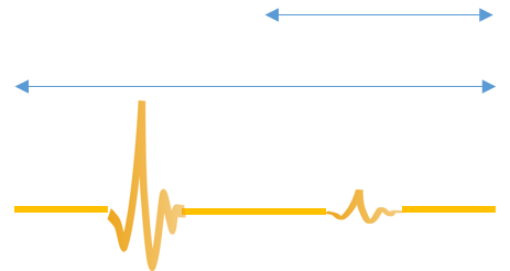
Figure 1: We first apply a matched-filter to the whole recorded signal to detect the largest peak. After finding the larger peak, we truncate the signal and apply the filter to the truncated version in order to find the smaller one.

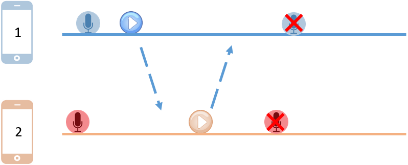
Figure 2: Elapsed time between two times of arrivals (ETOA) method: both phones start recording (indicated by microphone icon), emit a pulse each (play icon), and finally stop recording.

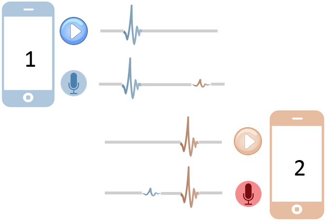
Figure 3: Phone 1 sends a pulse, phone 2 responds to it with another pulse, everything has been recorded by both phones. The play icon represents what the phones are emitting, th microphone icon what the phones are recording.

3.3 Assumptions and Parameter Selection

The sampling rate $f_{s}$, recording length and speed of sound $\nu_{s}$ influence the performance of acoustic ranging.

The sampling rate is very important because it determines the maximum frequency and bandwidth that can be used. Because the audio hardware of the smartphones are designed to play in audible frequency range, the highest possible sampling frequency for most of the phones are 48 kHz [9]. Since according to Nyquist’s theorem a higher sampling rate implies a higher bandwidth, we thus choose $f_{s}=48$ kHz.

The recording length is very important since a short duration can cause phones to miss pulses. On the other hand, longer recordings need more memory and the detection requires more computation. So there is a trade-off between the length of the recording and the chance of missing pulses.

To circumvent this issue, we use a simple communication protocol, illustrated in Figure 2. This protocols works over the existing Wi-Fi network. The phones let each other know via a WiFi connection that they started recording. After the reception of this message phone 1 emits its acoustic pulse. To ensure that phone 1 does not record indefinitely, phone 2 passes a message to phone 1 after it played the pulse. As soon as phone 1 receives it, it stops recording. This way we are sure that both phones have recorded both pulses and no one misses anything. It means that the recording length is not a constant and it varies according to the OS delays and network delays.

Acoustic distance measurement depends on the speed of sound, which is temperature dependent. Some recent smartphones have temperature sensors. Using this they can calculate the speed of sound according to the temperature sensor. As the phones we used, Samsung Galaxy S4 Mini, are not equipped with such a sensor, we assign the speed of sound according to the average room temperature of around $25^{\circ}C$, i.e., $\nu_{s}=340\,m/s$.

In brief, we built an Android Phone App for acoustic ranging using ETOA measurement with sample counting and self-recording to calculate the distance between two phones using the above. Figures 2 and 3 illustrate the basic mechanisms.

4 Multiple-Node Localization

Above, we discussed how to measure distances between two devices using acoustics. Furthermore we described how Euclidean Distance Matrices (EDMs) can be used to infer positions under ideal conditions in Section 2.3. We now explain how to use these as building blocks to localize several phones simultaneously under noisy conditions.

First, we describe our method to collect pairwise distances efficiently, followed by the description of the pulse shape and detection design we used. Subsequently, we discuss how to position several devices simultaneously despite incomplete and noisy EDMs.

4.1 Central Distance Collection

We cannot use the application described in Section 3 to measure the pairwise distances between several phones as is. With an increasing number of phones, several issues arise.

Let $N$ be the number of phones. There are $N\choose 2$ pairwise distances to be measured. If we measure one distance at a time and each measurement takes $T_{m}$ milliseconds, we need $T_{m}N(N-1)/2$ in total to do all the measurements. If the location of some phones change during this time, we get measurements which do not correspond to the same positioning of the phones. Therefore, the total measurement time should be short as much as possible to guarantee that the measured values correspond to one configuration of the phones. Otherwise, we cannot use the distances to form an EDM. Therefore, instead of doing individual pairwise measurements, we propose a scheme to do all the measurements in one interval.

Clearly, the number of calculations to be executed by each phone increases as the number of phones grows. Also there is an extra calculation that we do not have in acoustic ranging, namely solving the MDS problem. Even though this can be done in a distributed way efficiently, it requires that each phone knows the pairwise distances of all nodes, which requires the exchange of $O(N^{2})$ messages. Thus we decided to carry out all computations on a server, which incurs a linear message complexity of $O(N)$ and also reduces battery power consumption in the phones.

In addition, the server is not only used for collecting data and doing the calculations, it can also schedule the localization related activities and minimize the probability of missed pulses or of two pulses of two phone colliding.

Here, we summarized the main responsibilities of the server:

• Schedule the pulse emitting procedure.

• Collect recordings from the phones.

• Calculate distances and EDMs.

• Run algorithms to solve the MDS problem and localize phones.
  

For the measurements, each phone carries out the following steps.

1. Start recording when receiving LISTEN($t_{1},t_{2}$) command from the server via a WiFi link.

2. Play pulse after time $t_{1}$.

3. Stop recording after time $t_{2}$ has elapsed.

4. Send the recording to the server a WiFi link.
   

Ideally, in each phone’s recording we have $N$ different recorded pulses. If we can detect these pulses in each recording, we can find the Round Trip Time (RTT) for each pair. The recorded signal of phone $i$ can be written as

$$r_{i}[n]=\sum_{j}s_{j}[n-T_{i,j}],$$ (11)

where $s_{j}(.)$ is the received signal from phone $j$ and $n$ is the index of the $n^{th}$ sample of a signal. $T_{i,j}$ is the index of the sample which corresponds to the time phone $i$ receives the pulse from phone $j$. For simplicity and because we are only interested in differences, not in absolute time, we can assume here that all the phones started the recording at the same time. The distance between phone $i$ and $j$ can thus be computed as

$$d_{i,j}=\frac{|(T_{i,j}-T_{i,i})-(T_{j,j}-T_{j,i})|}{2f_{s}}\nu_{s},$$ (12)

where $\nu_{s}$ is the speed of sound and $f_{s}$ is the sampling frequency. Figure 4 illustrates why this formula is true, even if the ordering of pulses leads to negative $\Delta_{2}$.

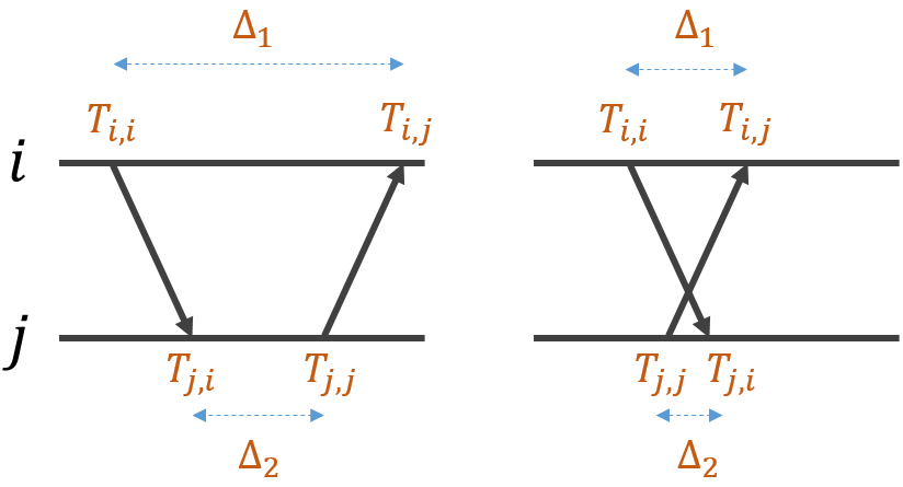
Figure 4: (left) RTT $=\frac{\Delta_{1}-\Delta_{2}}{2}$. (right) RTT $=\frac{\Delta_{1}+\Delta_{2}}{2}$.

4.1.1 Scheduling: Increasing Reliability

There are several factors that can cause errors in the measurements, falling in one of the two categories.

• Android OS and networking delay (missed pulse error).

• Acoustics errors (NLOS components, reverberations, obstruction).

Consider for example the case where a phone starts recording too late because of delays introduced by the Android OS and thus misses the pulses of other phones. Analogously, a phone can stop recording too early and miss pulses. A good schedule can minimize the probability of such errors.

Let $S=\{(t_{1}^{(1)},t_{2}),(t_{1}^{(2)},t_{2}),\ldots,(t_{1}^{(N)},t_{2})\}$ denote a schedule that tells phone $i$ to emit its pulse $t_{1}^{(i)}$ ms after the reception of the message and to stop recording after $t_{2}$ ms. The server determines the schedule $S$ and broadcasts it to the $N$ involved phones over the WiFi network. Let $delay_{OS}$ be a bound on the maximum delay cause by the operation system and networking. To avoid errors, the schedule computed by the server should satisfy some conditions.

1. $\forall i:~{}t_{1}^{(i)}>delay_{OS}$ (to avoid late recording errors)

2. $\min_{i}(t_{2}-t_{1}^{(i)})>delay_{OS}$ (to avoid early stopping errors)

3. $\forall i,j:\>|t_{1}^{(i)}-t_{1}^{(j)}|>\delta$ (to avoid colliding pulses)
   

We choose $t_{j}^{(i)}$s for $N$ phones in the following way

$$t_{1}^{(i)} = D_{delay}+i\cdot D_{0}.$$ (13)

$$t_{2} = 2\cdot D_{delay}+N\cdot D_{0}.$$ (14)

The reason why we separate $t_{1}^{(i)}$into two terms is the fact that there are two different types of error. The first type is to miss pulses and the second one is the collision of pulses. To prevent the former, we force the phones to wait for an amount of time, i.e. $D_{delay}$, before the first one sends a pulse to decrease the probability of missing any pulses because not all phones are in the recording state yet. We determined experimentally that $D_{delay}=100$ ms is a good choice taking OS and networking delay into account. Collision errors are avoided by an additional amount of delay that varies from phone to phone, i.e. phone $i$ waits $iD_{0}$ time before playing its pulse (assuming a pulse duration below $D_{0}$). To minimize the collision probability under i.i.d. OS and networking delay, given measurement time $t_{2}$, we set $D_{0}=(t_{2}-2D_{delay})/N$. Thus, by increasing $t_{2}$, the recording phase is extended, while the error probability is reduced. However, the probability that the phones have changed their positions in the meantime increases and higher storage and computation costs are induced.

Another option to increase the probability of success is to repeat the measurements and to combine the results (weighted averages). In particular, one can ask the following question.

For a given total length of a measurement interval $L_{T}$, what is the repetition rate that gives the least possible error?

In other words, what is the best choice for the number of repetitions $m^{*}$, such that

$$m^{*}=arg\min_{m}\mathbb{P}_{\text{error}}(L)^{m}$$ (15)

where $\mathbb{P}_{\text{error}}(L)$ is the probability of error for the length of measurements $L$ and $L=\lfloor\frac{L_{T}}{m}\rfloor$. To this end, we discuss in Section 4.3 how to fuse several (potentially incomplete) EDMs to get a better accuracy result, i.e. optimum weightings. Given a set of assumptions one can thus optimize along the trade-off between the required time for the measurements and the accuracy. However, this is out of the scope of this article. In our evaluation section we show that 5 repetitions provide an error margin of around 15cm in a noisy office environment.

Consequently, instead of using $N(N-1)$ pairwise recordings with up to two pulses each, we use one recording interval at each device with containing up to $N$ pulses. This minimizes time and coordination, enabling evaluation in less than $1s$.

4.2 Pulse Shape and Detection Scheme

The detection scheme described in Section 3 for acoustic ranging does not satisfy all requirements for a multi-phone setting. Since we want to carry out all pairwise measurements together, two important issues arise:

• For $N$ phones, we need $N$ different pulse shapes that are easily distinguishable because we would like to find their positions in each recording and compute their corresponding $T_{i,j}$s.

• Each phone receives not only different pulses but also with different power levels. This means that a recorded signal, contains $N$ different pulses where the corresponding power depends on the distance between this phone and the other ones. The detection scheme should thus not be sensitive to the power level.

These two issues are related. In theory, if we have orthogonal pulse shapes in the recorded signal, we can detect them without too much trouble because

$$\langle s_{i}[n],s_{j}[n]\rangle=\delta_{ij}R_{j}[0]$$ (16)

where $s_{i}(t)$ is the pulse of phone $i$. The output of the matched filter detector for pulse $j$ is

$$\begin{split}y_{i,j}[n]&=\sum_{n^{\prime}}r[n^{\prime}]s_{j}[n^{\prime}+n]\\ &=\sum_{n^{\prime}}\sum_{m}a_{i,m}s_{m}[n^{\prime}-T_{i,j}]s_{j}[n^{\prime}+n]\\ &=a_{i,j}R_{j}[n-T_{i,j}]\end{split}$$ (17)

where $R_{j}[n]$ is the autocorrelation of pulse $j$ and $a_{i,j}$ is the amplitude of the received pulse $j$ by phone $i$. The last equality holds because of (16). Since the maximum value of the autocorrelation function is $R_{j}[0]$, it is easy to determine $T_{i,j}$ by finding the maximum value of the output. In this case, having different power levels is no longer a problem.

In practice, there are several factors such as noise and imperfect orthogonality that make the amplitude of the received signal important for detection. In a more general case where the orthogonality does not hold, we get

$$y_{i,j}[n]=a_{i,j}R_{j}[n-T_{i,j}]+\sum_{m\neq j}a_{i,m}R_{i,m}[n-T_{i,m}],$$ (18)

where $R_{i,m}[n]$ is the cross-correlation function of pulses $s_{i}[.]$ and $s_{m}[.]$. We had this issue for two phone distance meter too and we solved it using a heuristic approach. However, when the number of phones increases and there is no tight coordination between the phones to send pulses (unlike the case with only two phones), we cannot use that method because we do not know anything about $a_{i,j}$s and how they compare to each other.

One possible solution is to detect the pulses iteratively. We can detect one pulse at a time and then cancel its contribution from the recorded signal. We repeat this procedure on the canceled recording in the previous step for another pulse recursively.

For example, suppose there are only two phones. Hence, we have two pulses in each recording. To detect these pulses we can first detect the larger one. Subtracting this pulse from the recording results in a signal that only contains one pulse (smaller one). Now we can easily detect the smaller one without thinking about the cross-correlation term $R_{1,2}[.]$ because we have already removed the larger pulse.

Again, this methods would work perfectly if the pulses were not distorted and noise free. In practice, we have still a residual of larger pulse after cancellation.

4.2.1 Pseudo-Random Binary Sequences

In principle any pulse shape with a narrow autocorrelation function can be used in such a localization system. Due to the constraints posed by the built-in microphone and speaker, we select Pseudo-noise (PN) sequences in the frequency range 15-20 kHz and durations of 1000 samples. Though 15 kHz is still audible by humans, it is noticed only as a very short pulse. PN sequences have a large bandwidth with a narrow autocorrelation function. These characteristics depend on the length of the sequence and facilitate detection. The longer the sequence, the better the detectability.

As the phones receive signals from other phones as well as the one emitted by themselves, the signals vary in their power levels. To avoid the problem of different power levels if we use the traditional matched filter approach, we propose a CDMA-like detection scheme that correlates a binary signal to detect pulses. A PN binary pulse shape of length $L$ is defined as

$$s[n]=b_{n}\quad for\quad n=0,2,\dots,L-1,$$ (19)

where $b_{n}$s are realizations of i.i.d. binary random variables with $P(b_{n}=1)=P(b_{n}=-1)=\frac{1}{2}$. These sequences are suitable as they do not convey any information in their amplitude. Hence, additive noise with reasonable variances can be canceled easily by a sign filter. Thus, we can ignore the amplitude and apply the matched filter detection on a binary sequence.

The proposed detection scheme is illustrated in Figure 5. On the transmitter part, we first upsample the generated PN binary sequence by a factor of $P$. For the inserted zeros by upsamplers, we interpolate the values. The resulting pulse is our new pulse shape. We do the interpolation and upsampling to decrease the required bandwidth and make it lowpass. Therefore, we used $P=4$ to reduce the bandwidth and be able to modulate the signal to higher frequencies. However, for very high frequencies, greater than 20 kHz, audio components are more affected by distortions caused by the microphone and loud speaker.

On the receiver side, instead of directly applying a matched filter that corresponds to the transmitted pulse shape, we pass it through a sign filter. Then we apply a matched filter that corresponds to the signed version of the pulse shape. The output of the matched filter will be fed into a peak detector in order to find $T_{i,j}$s.

The proposed detection scheme shows a better performance compared to using a matched filter directly. Though it may be surprising at the first glance, this is due to the lack of the optimality condition for the matched filter. The matched filter receiver is the optimum linear filter in the sense of SNR. However, in this case we do not know the distortion by the acoustic propagation channel, therefore a matched filter based on only the pulse shape does not necessarily work better in all circumstances.

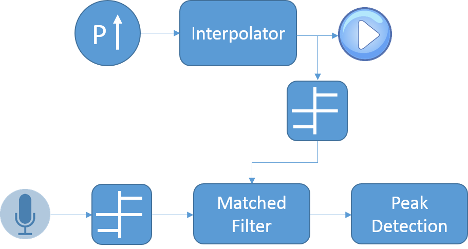
Figure 5: Transmitter (top) and receiver (bottom) of detection scheme

4.3 Robust Positioning with incomplete EDMs

We cannot use the classical method of multi-dimensional scaling discussed in Section 2.3, as pairwise distance measurements are noisy or might even be missing if two phones are too far from each other to detect each other’s pulse. There exist optimization-based methods to solve the MDS problem for incomplete EDMs. A common cost function to solve this problem is called raw Stress function [14]:

$$\min_{\mathbf{X}\in\mathbb{R}^{N\times\eta}}\sum_{i,j}w_{i,j}\left(\sqrt{\mathbf{D}(\mathbf{X})[i,j]}-d_{i,j}\right)^{2}$$ (20)

This cost function lets us cope with situations where some of the distances are not given. We can set $w_{i,j}$ to zero if $d_{i,j}$ is not given. Unfortunately, the raw Stress function is non-convex also it is not globally differentiable so the optimization methods for solving it are rather involved.

Thus, we use a convex cost function called s-stress to solve the MDS problem despite incomplete EDMs as proposed by Takane et al. [23]:

$$\min_{\mathbf{X}\in\mathbb{R}^{N\times\eta}}\sum_{i,j}w_{i,j}\left(\mathbf{D}(\mathbf{X})[i,j]-d_{i,j}^{2}\right)^{2}$$ (21)

Contrary to the raw Stress function, the s-stress function is convex and differentiable everywhere. However, it favors long distances over shorter ones. When $\eta=N-1$, an algorithm by Gaffke and Mathar [8] can find the global minimum of the s-stress function. We are interested in cases where the number of spatial dimensions $\eta$ ($\eta=2$ or $3$) is significantly smaller than the number of nodes $N$. Parhizkar [18] proposed an algorithm to minimize this function in a (distributed) manner based on the alternating gradient descent optimization method, see Algorithm 2. In each iteration it uses the coordinate descent method by optimizing along one of the variables cyclically. To the best of our knowledge, no other MDS methods combine 1) operation without parameter-tuning, 2) configuration independence, 3) fast convergence, and 4) cope with missing/noisy data.

Algorithm 2 Alternating coordinate descent method for minimizing the s-stress function [18]

Input: Distance matrix $\tilde{\mathbf{D}}$.
Output: Estimated positions $\hat{\mathbf{X}}$.

1:Assume an initial configuration for the sensors $\mathbf{X}_{0}$.

2:repeat

3:     for sensor number $i=1$ to $N$ do

4:         Assume the configuration of the rest of the sensors fixed;

5:         Use the coordinate descent method to find the $x$ coordinate of sensor $i$ using distance information of its neighbors;

6:         Use the coordinate descent method to find the $y$ coordinate of sensor $i$ using distance information of its neighbors;

7:         Send the estimated position of sensor $i$ to its neighbors;

8:     end for

9:until convergence or maximum number of iterations is reached.

This algorithm has the advantage that it lets us fuse several sets of measurements easily. Thus, we can increase the accuracy by repeating the experiment several times. When there are only two phones, we can simply take the average over the measured values. Now, suppose we have repeated the measurements for multiple-node localization and obtained several EDMs, one per measurement. The naive approach is to average over each component separately and form a new EDM. We can feed this new EDM into Algorithm 2 to minimize the cost function in (21). In other words, this new EDM contains the mean value of the measured distances. We improve over the naive approach by weighting the measurements. By modeling the measurement noise as additive Gaussian noise, one can show that if we choose the weight $w_{i,j}$ inversely proportional to the squared variance of the measurements between node $i$ and $j$, the error is minimized, i.e.

$$w_{i,j}=\frac{1/\sigma_{ij}^{4}}{\sum_{i^{\prime},j^{\prime}}1/\sigma_{i^{\prime},j^{\prime}}^{4}}.$$ (22)

A lower weight reflects a higher variance which means more uncertainty in measuring the corresponding distance. Since we do not know the exact variances of the measurements, we estimate it by the sample variance.We evaluated both the naive and the optimum weighting strategy in Section 5.2.

4.4 Application and Server Design

The Android application on the phone communicates with the server using a socket connection over Wi-Fi. The first time a phone connects to the server it registers itself and goes into waiting mode. Upon a localization request, the server computes a schedule and broadcasts a separate message with schedule information to each registered phones. They start recording as soon as they received the message. Each phone plays a generated pseudo-random binary pulse of length $L$ after a certain delay as assigned by the schedule of the server. They stop recording according to the received schedule and send their recorded signal to the server over the wireless link.

The server collects all the recordings and processes the collected data to determine the location of the phones. We implemented our server with Node.JS, which is based on Chrome’s JavaScript runtime for building fast, scalable network applications. It is lightweight, platform-independent and well-suited for data-intensive real-time applications. Our application exchanges data in JSON format, an open standard format that uses human-readable text to transmit data objects consisting of attribute-value pairs. For the calculation of the position, our Node.JS script calls a server-side MATLAB application, allowing for fast prototyping and easy plotting.

5 Evaluation

5.1 Acoustic Ranging

One of the important factors to evaluate an indoor localization system is its accuracy. Let us first compare the performance of the single tone method described in Section 3.2 to the CDMA-like approach of Section 4.2, depicted in Figure 6. In the single tone approach, we used two sinusoidal pulses at frequencies 18 and 19 kHz for each phone. The accuracy and confidence are much better for the binary PN sequence.

Figure 6: Error vs the actual distance for the finite duration sinusoid (left) and PN sequence (right) schemes: average and standard deviations of 10 measurements with phones at distance 0.1m, 0.5m and 1.5m from each other.

Due to this and the reasons explained in Section 4.2, we used PN sequences in the remainder of our evaluation. To see how accurate our ranging algorithm is, we applied the proposed ranging method with binary PN sequences on distances up to 6.5m.

Figure 7: Accuracy of the range measurement scheme with PN sequences. The error and standard deviation is based on 10 measurements per distance.

Figure 7 shows that the accuracy is around 5cm in this case. Note that the data for this plot has been acquired on a different day than the data for Figure 6, therefore the conditions such as temperature etc. differ and also the results are slightly different. As expected, the confidence level for longer distances is higher than distances below 1 m. The confidence intervals for such accuracy is around 4 cm in the worst case. Thus the error for longer distances is surprisingly low, i.e., in the order of only 1%. This is due to the fact that we removed distance values exceeding 8m as outliers, since they are beyond the effective range of our parameter settings for the ETOA approach. Naturally, this has a larger effect when the actual distance is larger.

Figure 8: Examples with one measurement set. Red asterisks correspond to actual, blue circles to estimated locations. (a) and (c) 5 resp. 6 phones in a quiet empty room, (b) and (d) 5 resp. phones in an office environment (in meter).

5.2 Acoustic Multiple-Node Localization

Here, we show the results of applying the localization scheme explained in the previous section in four different settings. We localized the phones in two configurations, a cross-shaped configuration of 5 phones where all the distances are mid-range and a three by three configuration of 6 phones where the distances are short-range and long-range. We repeated the experiment in two indoor environments: an empty quiet room. and an office environment with several people, computers, desks and other obstacles and noise.

In Figure 8, an example of the result obtained from one set of measurements for each configuration is depicted. As expected, the accuracy in an office is lower because of the obstacles and noise in the environment. It is impossible to keep all influencing factors the same in the two environments. For example the quality of the Wi-Fi network, which has a great effect on the delays with which the phones start recording, varies considerably. The error of the examples in Figure 8 is shown in Table 1 in centimeter. The error is the average deviation from the actual positions, i.e.

$$e=\frac{1}{N}\sum_{i=1}^{N}\|\hat{\mathbf{x}}_{i}-\mathbf{x}_{i}\|,$$ (23)

where $\hat{\mathbf{x}}_{i}$ and $\mathbf{x}_{i}$ are the estimated and actual positions respectively and rotation and translation have been applied for error minimization. The second setup, consisting of 6 phones, shows a better overall performance especially in the office. This might be due to the fact that the number of phones has a great impact on the performance of the MDS algorithm in [18]. However, more experiments are needed to verify this hypothesis. The overall accuracy is on the decimeter level.

Table 1: Error comparison (single measurement set).

	Cross-shaped	Three-by-Three
Empty room	1.30 cm	5.2 cm
Office	34.8 cm	8.2 cm

To increase the accuracy, several measurements can be carried out and combined, as described in Section 4.3. We evaluate mitigation of the influence of acoustic errors by repeating measurements in three different setups: short range, medium range and long range. Figure 9(a) shows the averaged distance versus the number of measurements for 10cm distance, while Figures 9(b) and 9(c) do the same for 1.6m and 6.4m respectively. As expected the short-range setup exhibits lower variance with hardly any outlier values. Our results indicate that a small number of repetitions, e.g., 5 measurements, is sufficient to achieve good accuracy.

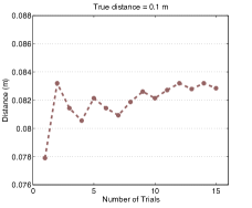
Figure 9: Calculating distances between two phones by averaging over several measurements (trials). The filled circles represent the average distance over x trials. (a) Distance 10cm: mean value of 15 measurements is 8.3 cm with 0.5 cm standard deviation. (b) Distance 1.6 m: mean value of 15 measurements is 1.64 m with 0.019m standard deviation. (c) Distance 6.4 m: mean value of 15 measurements is 6.34 m with 0.021m standard deviation.

(a) Cross-shaped

(b) Three-by-Three

Figure 10: Example of localization results using the optimum weighting scheme for 5 measurement sets in noisy office.

Table 2: Comparison of error for different weightings in noisy office (5 sets of measurements).

	Equal Weighting	Optimum Weighting
Cross-shaped	19.89 cm	13.6 cm
Three-by-Three	11.4 cm	9.7 cm

For multiple-node localization, the effect of repeating measurements depends on the weighting strategy. The average distance error is shown in Table 2. Compared to the results using one set of measurements we observe that error can be reduced up to 50%. The optimal weighting scheme outperforms the equal weighting scheme by up to 30%. In summary, our localization scheme behaves as expected and is able to provide error bounds of around 30cm in noisy environments using one set of measurement or around 15cm when combining several measurements.

6 Related Work

Many different indoor localization systems are available today, based on pedestrian dead-reckoning, Wi-Fi or other radio signals, cameras, etc. or a combination thereof. We refer to [17] for an overview. We focus here on describing ranging and positioning systems using acoustics.

The fact that many devices can generate sound from their built-in speaker and detect sound with the integrated microphone has been used in a number of different approaches. There are distance-free localization methods which use audio devices to capture acoustic impulse response as an input to a pattern classification algorithm, e.g. [20]. Here, we focus on the distance-related methods. The sound propagation is slow, compared to the speed of radio signals; thus time stamping signals is easier. Moreover, received signals can be analyzed in detail and the suppression of multipath signals is easier for acoustic signals than for radio signals. This helps to increase the accuracy compared to other methods.

In the following we describe existing acoustic ranging and positioning systems. While there is a multitude of the former, using different pulse shapes and calculation methods, the second has not received the same amount of attention. From a system design perspective, it is highly valuable to know how to schedule distance measurements between several nodes with unknown positions and how to process the results to derive positions. To the best of our knowledge, the current literature does not address these issues.

A large body of work on ranging has been developed in recent years. Among them BeepBeep [19] uses smartphones to emit and receive chirp pulses between 2 kHz and 6 kHz. The system needs no additional infrastructure and uses the Round Trip Time (RTT), ETOA and a matched filter to measure the distance with an accuracy of around 1cm. In [1], authors used Time-difference-of-arrivals (TDOA) and dual-carrier sinusoid with 500 Hz frequency shift as a pulse shape to locate a single smartphone. The indoor localization system Guoguo [15] uses doublet pulse between 15 and 20 kHz and Hadamard codes to identify the location of a smartphone. It uses beacons transmitted by special hardware and TOA to find the position. Other studies focus more on the system design of a localization framework, e.g., Beep [16], TOA-based localization system which finds the location of a sound source in 3D using Non-linear Least Square Estimation (NLSE). ASSIST [12] uses devices that receive chirp pulses between 18 kHz and 21 kHz transmitted from a smartphone to locate it. WALRUS [2] uses sound emitted from PDAs/Laptops at a frequency of 21 kHz to identify their location within a room. Hennecke et al. presented a method for the acoustic self-localization of nodes in an ad-hoc array of COTS smartphones. The smartphones worked in the audible range with a short chirp impulse between 5 kHz and 16 kHz. The audio signals were received by the smartphone microphone [11]. Liu et al. [15] proposed several approaches to improve pulse transmission and achieved 23 cm accuracy by averaging over several measurements. Marziani et al. [6] use an RTT and CDMA-based method, to provide a distributed architecture on specialized devices to find pairwise distances. However, they do not determine the actual positions of the nodes. Chakraborty et al. [3] presented a TDOA-based localization scheme on ZigBee modules to determine the location of a sound source with respect to nodes at a known position. Their solution provides 60cm accuracy using Least Square Estimation (LSE). Another localization system using smartphones is Whistle [25], applying a ranging method similar to BeepBeep with 10-20 cm accuracy for localizing a sound source with TDOA. It is implemented on Windows phones and a server using the method described in [4] for solving non-linear TDOA equations to calculate the position of the source. The problem of finding the position of multiple nodes simultaneously using acoustics is not discussed in any of the work we are aware of.

7 Conclusions

In this article we proposed a localization system to position several phones simultaneously. Our system uses ETOA measurements with sample counting to compute distances between phones. We used the s-stress cost function to formulate the problem of finding the positions from the distances as an optimization problem to which we applied an alternating gradient descent algorithm. Furthermore, we described a pseudo-noise-based pulse shaping and detection scheme and a method to schedule multi-node measurements reliably despite OS and networking delays, which has not been addressed in other work to the best of our knowledge. In addition to reliability, accuracy is an important performance measure of a localization system. To improve the accuracy, we take measurements several times and combine them using an optimal weighting strategy.

While we used a centralized approach to do the computations, Algorithm 2 has the intrinsic capability to be implemented in a distributed way. The current scheme cannot be directly implemented on the phones in a distributed way because of its (message) complexity, therefore devising ways to decrease the complexity is a promising path of research. A more advanced system could also adapt its measurement strategy dynamically to changing network conditions and deal with non-line-of-sight (NLOS) components.

In summary, we want to stress that acoustics can be a powerful tool for indoor localization and positioning, especially when it is combined with other localization methods based on Wi-Fi or inertial sensors. How to fuse several of these approaches with acoustic-based methods is another interesting direction for further research.

References

- [1] T. Akiyama, M. Nakamura, M. Sugimoto, and H. Hashizume. Smart phone localization method using dual-carrier acoustic waves. In Indoor Positioning and Indoor Navigation (IPIN), 2013.
- [2] G. Borriello, A. Liu, T. Offer, C. Palistrant, and R. Sharp. Walrus: Wireless acoustic location with room-level resolution using ultrasound. In Conference on Mobile Systems, Applications, and Services (MobiSys), 2005.
- [3] J. Chakraborty, G. Ottoy, M. Gelaude, J.-P. Goemaere, and L. De Strycker. In Computer and Information Technology (ICCIT).
- [4] Y. Chan and K. Ho. A simple and efficient estimator for hyperbolic location. Signal Processing, IEEE Transactions on, 42(8):1905–1915, Aug 1994.
- [5] T. Cover and P. Hart. Nearest neighbor pattern classification. Information Theory, IEEE Transactions on, 13(1):21–27, January 1967.
- [6] C. De Marziani, J. Urena, A. Hernandez, J. Garcia, F. Álvarez, A. Jimenez, M. Perez, J. Carrizo, J. Aparicio, and R. Alcoleas. Simultaneous round-trip time-of-flight measurements with encoded acoustic signals. Sensors Journal, IEEE, 12(10):2931–2940, 2012.
- [7] V. Filonenko, C. Cullen, and J. D. Carswell. Indoor positioning for smartphones using asynchronous ultrasound trilateration. ISPRS International Journal of Geo-Information, 2(3):598–620, 2013.
- [8] N. Gaffke and R. Mathar. A cyclic projection algorithm via duality. Metrika, 36(1):29–54, 1989.
- [9] Google. Android documentation. http://developer.android.com/reference/android/media/package-summary.html, 2014.
- [10] S. Haykin. Digital Communication Systems. Wiley, 2013.
- [11] M. Hennecke and G. Fink. Towards acoustic self-localization of ad hoc smartphone arrays. In Hands-free Speech Communication and Microphone Arrays (HSCMA), 2011 Joint Workshop on, pages 127–132, May 2011.
- [12] F. Hoflinger, R. Zhang, J. Hoppe, A. Bannoura, L. Reindl, J. Wendeberg, M. Buhrer, and C. Schindelhauer. In Indoor Positioning and Indoor Navigation (IPIN).
- [13] J. Kruskal. Multidimensional scaling by optimizing goodness of fit to a nonmetric hypothesis. Psychometrika, 29(1):1–27, 1964.
- [14] J. Kruskal. Nonmetric multidimensional scaling: A numerical method. Psychometrika, 29(2):115–129, 1964.
- [15] K. Liu, X. Liu, L. Xie, and X. Li. Towards accurate acoustic localization on a smartphone. In INFOCOM, 2013.
- [16] A. Mandal, C. Lopes, T. Givargis, A. Haghighat, R. Jurdak, and P. Baldi. Beep: 3d indoor positioning using audible sound. In Consumer Communications and Networking Conference, 2005.
- [17] R. Mautz. Indoor positioning technologies. ETH Zurich, Department of Civil, Environmental and Geomatic Engineering, Institute of Geodesy and Photogrammetry, 2012.
- [18] R. Parhizkar. Euclidean distance matrices: Properties, algorithms and applications. PhD thesis, ÉCOLE POLYTECHNIQUE FÉDÉRALE DE LAUSANNE, 2013.
- [19] C. Peng, G. Shen, Y. Zhang, Y. Li, and K. Tan. Beepbeep: A high accuracy acoustic ranging system using cots mobile devices. In Conference on Embedded Networked Sensor Systems (Sensys), 2007.
- [20] M. Rossi, J. Seiter, O. Amft, S. Buchmeier, and G. Tröster. Roomsense: An indoor positioning system for smartphones using active sound probing. In Proceedings of the 4th Augmented Human International Conference, Mar. 2013.
- [21] I. J. Schoenberg. Remarks to Maurice Fréchet’s article “Sur la définition axiomatique d’une classe d’espaces distances vectoriellement applicable sur l’espace de Hilbert”. Annals of Mathematics 36(3), 1935.
- [22] Y. Shang, W. Ruml, Y. Zhang, and M. P. J. Fromherz. Localization from mere connectivity. In Proceedings of the 4th ACM International Symposium on Mobile Ad Hoc Networking &Amp; Computing, MobiHoc ’03, pages 201–212, New York, NY, USA, 2003. ACM.
- [23] Y. Takane, F. Young, and J. Leeuw. Nonmetric individual differences multidimensional scaling: An alternating least squares method with optimal scaling features. Psychometrika, 42(1):7–67, March 1977.
- [24] B. Vucetic and S. Glisic. Spread Spectrum CDMA Systems for Wireless Communications. 1997.
- [25] R. Yu, B. Xu, G. Sun, and Z. Yang. Whistle: synchronization-free tdoa for localization. In J. Beutel, D. Ganesan, and J. A. Stankovic, editors, SenSys, pages 359–360. ACM, 2010.