Moduli space of cubic Newton maps

Abstract.

In this article, we study the topology and bifurcations of the moduli space $\mathcal{M}_{3}$ of cubic Newton maps. It’s a subspace of the moduli space of cubic rational maps, carrying the Riemann orbifold structure $(\mathbb{\widehat{C}},(2,3,\infty))$. We prove two results:

$\bullet$ The boundary of the unique unbounded hyperbolic component is a Jordan arc and the boundaries of all other hyperbolic components are Jordan curves;

$\bullet$ The Head’s angle map is surjective and monotone. The fibers of this map are characterized completely.

The first result is a moduli space analogue of the first author’s dynamical regularity theorem [Ro08]. The second result confirms a conjecture of Tan Lei.

1. Introduction

Let $P$ be a polynomial of degree $d\geq 2$. It can be written as

$$P(z)=a_{d}z^{d}+a_{d-1}z^{d-1}+\cdots+a_{1}z+a_{0},$$

where $a_{0},\cdots,a_{d}$ are complex numbers and $a_{d}\neq 0$. The Newton’s method $N_{P}$ of $P$ is defined by

$$N_{P}(z)=z-\frac{P(z)}{P^{\prime}(z)}.$$

The method, also known as the Newton-Raphson method named after Isaac Newton and Joseph Raphson, was first proposed to find successively better approximations to the roots (or zeros) of a real-valued function. In 1879, Arthur Cayley [C] first noticed the difficulties in generalizing the Newton’s method to complex roots of polynomials with degree greater than 2 and complex initial values. This opened the way to study the theory of iterations of holomorphic functions, as initiated by Pierre Fatou and Gaston Julia around 1920. In the literature, $N_{P}$ is also called the Newton map of $P$. The study of Newton maps attracts a lot of people both in complex dynamical systems and in computational mathematics.

1.1. What is known

The Newton maps can be viewed as a dynamical system as well as a root-finding algorithm. Therefore, it provides a rich source to study from various purposes. Here is an incomplete list of what’s known for Newton maps from different views:

Topology of Julia set: The simple connectivity of the immediate attracting basins of cubic Newton maps was first proven by Przytycki [P]. Shishikura [Sh] proved that the Julia sets of the Newton maps of polynomials are always connected by means of quasiconformal surgery. Applying the Yoccoz puzzle theory, Roesch [Ro08] proved the local connectivity of the Julia sets for most cubic Newton maps.

The combinatorial structure of the Julia sets of cubic Newton maps was first studied by Janet Head [He]. With the help of Thurston’s theory on characterization of rational maps, Tan Lei [Tan] showed that every post-critically finite cubic Newton map can be constructed by mating two cubic polynomials; Building on the thesis [Mi], Lodge, Mikulich and Schleicher [LMS1, LMS2] gave a combinatorial classification of post-critically finite Newton maps.

Root-finding algorithm: As a root-finding algorithm, Newton’s method is effective for quadratic polynomials but may fail in the cubic case. McMullen [Mc1] exhibited a generally convergent algorithm (apparently different from Newton’s method) for cubics and proved that there are no generally convergent purely iterative algorithms for solving polynomials of degrees four or more. On the other hand, by generalizing a previous result of Manning [Ma], Hubbard, Schleicher and Sutherland [HSS] proved that for every $d\geq 2$, there is a finite universal set $S_{d}$ with cardinality at most ${O}(d\log^{2}d)$ such that for any root of any suitably normalized polynomial of degree $d$, there is an initial point in $S_{d}$ whose orbit converges to this root under iterations of its Newton map. For further extensions of these results, see [S] and the references therein.

Beyond rational maps: The dynamics of Newton’s method for transcendental entire maps are intensively studied by many authors. Bergweiler [Be] proved a no-wandering-domain theorem for transcendental Newton maps that satisfy some finiteness assumptions. Haruta [Ha] showed that when the Newton’s method is applied to the exponential function of the form $Pe^{Q}$ (where $P,Q$ are polynomials), the attracting basins of roots have finite area. For the Newton maps of entire functions, Mayer and Schleicher [MS] showed that the immediate basins are simply connected and unbounded; Buff, Rückert and Schleicher further investigated the dynamical properties of these maps, see [BR, RS]. For the higher dimensional cases, Hubbard and Papadopol [HP], Roeder [Ro] studied the Newton’s methods for two complex variables.

1.2. Main results

Most above known results share a common feature. They focus on the dynamical aspect of the Newton maps. In this paper, we study the topology and bifurcations in the moduli space.

We first give some notations. Let $f$ be a rational map, ${\rm Aut}(\mathbb{\widehat{C}})$ be the group of Möbius transformations. We use $[f]=\{\phi f\phi^{-1};\phi\in{\rm Aut}(\mathbb{\widehat{C}})\}$ to denote the Möbius conjugate class of $f$.

It is worth observing that for any polynomial $P$ of degree $d\geq 2$, a simple root of $P$ corresponds to a super-attracting fixed point of its Newton map $N_{P}$, and that $N_{P}$ and $P$ have the same degree if and only if $P$ has $d-1$ distinct roots. The moduli space of degree $d$ Newton maps, denoted by $\mathcal{M}_{d}$, is defined as the following set

$$\{[N_{P}];P\text{ is a degree $d$ polynomial with $d-1$ distinct roots}\}$$

endowed with an orbifold structure. A point $\tau=[f]\in\mathcal{M}_{d}$ is said hyperbolic if the rational map $f$ is hyperbolic (i.e. all critical orbits of $f$ are attracted by the attracting cycles). It’s known that the hyperbolic set $\mathcal{M}_{d}^{hyp}=\{\tau\in\mathcal{M}_{d};\tau\text{ is hyperbolic}\}$ is an open subset of $\mathcal{M}_{d}$. A connected component of $\mathcal{M}_{d}^{hyp}$ is called a hyperbolic component.

The space $\mathcal{M}_{2}$ is trivial, it consists of a singleton because every Newton map of a quadratic polynomial with distinct roots is Möbius conjugate to the square map $z^{2}$, see [B]. The moduli space $\mathcal{M}_{3}$ of Newton maps of cubic polynomials with distinct roots is a non-trivial space with the lowest degree. It carries a Riemann orbifold structure (see $\S$ 2) and it has a unique unbounded hyperbolic component $\mathcal{H}$. The component $\mathcal{H}$ consists of the Möbius conjugate classes of cubic Newton maps $f$ for which the free critical point is contained in the immediate basin of a polynomial root. By quasiconformal surgery (see[Ro08, Remark 2.2]), one sees that $\mathcal{H}$ consists of points $\tau=[f]$ for which the cubic Newton map $f$ is quasiconformally conjugate to the cubic polynomial $z^{3}+3z/2$ near its Julia set, see Figure 3 (right) of the current paper. Thus all maps in $\mathcal{H}$ have polynomial dynamical behaviors, and they are not genuine cubic rational maps. The picture of the moduli space $\mathcal{M}_{3}$ (with a suitable parameterization) first appeared in Curry, Garnett and Sullivan’s paper [CGS, Fig. 3.1]. In [Tan], Tan Lei gave some descriptions of this space as well as the hyperbolic components.

The current paper is the continuation of the first named author’s work, where the following fundamental result [Ro08, Theorem 6] is proven:

Theorem 1.1 (Roesch [Ro08]).

For any cubic Newton map in $\mathcal{M}_{3}\setminus\mathcal{H}$ and with no Siegel disk, all the Fatou components are bounded by Jordan curves.

Our first main result is an analogue of Theorem 1.1 in the moduli space:

Theorem 1.2.

In the moduli space $\mathcal{M}_{3}$ of cubic Newton maps,

1. the boundary of the hyperbolic component $\mathcal{H}$ is a Jordan arc, and

2. the boundaries of all other hyperbolic components are Jordan curves.

Here, we say a set $\gamma$ is a Jordan curve (resp. Jordan arc) if it is homeomorphic to the circle $\mathbb{S}$ (resp. the open interval $(0,1)$). The reason that $\partial\mathcal{H}$ is a Jordan arc rather than a Jordan curve is that $\partial\mathcal{H}$ stretches towards the infinity ‘$\infty$’ (abstract point where the cubic Newton maps degenerate in the moduli space). This $\infty$ is exactly $[{(2z^{2}-z)}/{(3z-2)}]$, the Möbius conjugate class of the Newton map of cubic polynomial with double roots, say $z^{2}(z-1)$. Nevertheless, the one-point compactification $\overline{\mathcal{M}_{3}}=\mathcal{M}_{3}\cup\{\infty\}$ of $\mathcal{M}_{3}$ is a topological sphere and we will see in Section 9 that $\partial\mathcal{H}\cup\{\infty\}$ is a Jordan curve in $\overline{\mathcal{M}_{3}}$.

Theorem 1.2 is partially proven by the first named author in her thesis [R97], using parapuzzle techniques. The result and a sketch of proof were announced in [Ro99]. The current paper will present a complete proof, with methods different from parapuzzle techniques, allowing us to treat all hyperbolic components. The strategy of the proof follows the treatment of the McMullen maps in [QRWY]. The difference is, in the McMullen map case, both the dynamical plane and the parameter space have rich symmetries, allowing us to handle the combinatorial structure of the maps easily, however, for the cubic Newton maps, both the dynamical plane and the parameter space lack the symmetries, we need exploit the Head’s angle (see below) to classify the maps with different combinatorial structure. The complexity of the combinatorics makes the proof more delicate.

For each cubic Newton map $f$ with $[f]\in\mathcal{M}_{3}\setminus\mathcal{H}$, one can associate $f$ canonically with a combinatorial number, the Head’s angle $\boldsymbol{h}(f)\in(0,1/2]$ (see Section 5 for precise definition). As one will see in Section 5.1, this number characterizes how and where the two adjacent immediate basins of roots of the polynomial defining $f$ touch. It’s known [He, R97, Tan] that $\boldsymbol{h}(f)$ is contained in the set $\Xi$, which is defined by

$$\Xi=\{\theta\in(0,1/2];2^{k}\theta\in[\theta,1]\ ({\rm mod}\ \mathbb{Z})\text{ for all }k\geq 0\}.$$

The set $\Xi\cup\{0\}$ is known to be closed, perfect, totally disconnected and with Lebesgue measure zero, see [Tan, Prop 2.16]. Tan Lei [Tan] proved that every rational number $\theta\in\Xi$ can be realized as the Head’s angle of some cubic Newton map, by means of mating cubic polynomials and applying Thurston’s Theorem [DH2]. She conjectured [Tan, p.229, Remark] that each irrational angle $\theta\in\Xi$ can also be realized as the Head’s angle of some cubic Newton map.

Our second main result confirms this conjecture and characterizes the uniqueness of the realization:

Theorem 1.3.

Every angle $\theta\in\Xi$ can be realized as the Head’s angle of some cubic Newton map. This Newton map is unique up to Möbius conjugation if and only if $\theta$ is not periodic under the doubling map $t\mapsto 2t({\rm mod}\ \mathbb{Z})$.

Since the Head’s angle is invariant under Möbius conjugation, it induces a map, still denoted by $\boldsymbol{h}$, from $\mathcal{M}_{3}\setminus\mathcal{H}$ to $\Xi$. The map $\boldsymbol{h}$ is defined by sending the point $\tau=[f]\in\mathcal{M}_{3}\setminus\mathcal{H}$ to $\boldsymbol{h}(f)$. For any $\theta\in\Xi$, let $\boldsymbol{h}^{-1}({\theta})=\{\tau\in\mathcal{M}_{3}\setminus\mathcal{H};\mathcal{\boldsymbol{h}}(\tau)=\theta\}$ be the fibre of $\boldsymbol{h}$ over $\theta$. Let $\Theta_{per}$ and $\Theta_{dya}$ be the set of periodic and dyadic angles $\theta\in(0,1/2]$ under the doubling map $t\mapsto 2t({\rm mod}\ \mathbb{Z})$, respectively. They are written precisely as

$$\Theta_{per}=\{t\in(0,1/2];2^{k}t=t\ ({\rm mod}\ \mathbb{Z})\text{ for some }k\geq 1\},$$

$$\Theta_{dya}=\{t\in(0,1/2];2^{k}t=1\ ({\rm mod}\ \mathbb{Z})\text{ for some }k\geq 1\}.$$

It’s easy to check that $\Theta_{dya}\setminus\Xi\neq\emptyset$ and $\Theta_{per}\setminus\Xi\neq\emptyset$ (e.g. $5/16\in\Theta_{dya}\setminus\Xi,\ 2/7\in\Theta_{per}\setminus\Xi$). With these notations, Theorem 1.3 can be reformulated in terms of the mapping property of $\boldsymbol{h}$:

Theorem 1.4.

The Head’s angle map $\boldsymbol{h}:\mathcal{M}_{3}\setminus\mathcal{H}\rightarrow\Xi$ is surjective and monotone. Precisely,

1. if $\theta\in\Xi\cap\Theta_{per}$, then $\boldsymbol{h}^{-1}({\theta})$ is homeomorphic to $\overline{\mathbb{D}}\setminus\{1\}$;

2. if $\theta\in\Xi\setminus\Theta_{per}$, then $\boldsymbol{h}^{-1}({\theta})$ is a singleton.

Moreover, $\boldsymbol{h}$ is continuous at $\lambda$ if and only if $\boldsymbol{h}(\lambda)\in\Xi\setminus\Theta_{dya}$.

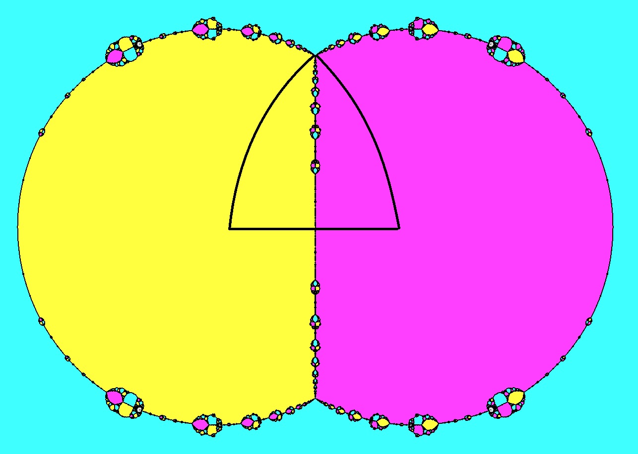
Figure 1. Head’s angle and the parameter space $\mathcal{X}$.

Let’s briefly describe the relation between the Head’s angle and the space $\mathcal{M}_{3}$, with the help of Figure 1. The space $\mathcal{M}_{3}$ is six-fold covered by the parameter space $\mathcal{X}=\mathbb{C}\setminus\{\pm\frac{3}{2},0\}$ of $N_{\lambda}(z)=\frac{2z^{3}-(\lambda^{2}-\frac{1}{4})}{3z^{2}-(\lambda^{2}+\frac{3}{4})}$ (see Section 2). There is a one-to-one correspondence between $\mathcal{M}_{3}$ and the region $\Omega$ (which is bounded by ray segments) plus some maps on the boundary $\partial\Omega$. As is shown in Figure 1, there are two main hyperbolic components: $\mathcal{H}_{0}^{1}$ (in yellow) and $\mathcal{H}_{0}^{2}$ (in purple). Their boundaries in $\Omega$ can be parameterized by the angles in $(0,1/2)$ (or $(1/2,1)$). The complementary $\Omega-\mathcal{H}_{0}^{1}\cup\mathcal{H}_{0}^{2}$ in $\Omega$ is a ‘string of beans’ (some kind of ‘Cantor necklace’), and each bean corresponds to a complementary interval of $\Xi$. The preimage of $\boldsymbol{h}$ either consists of a single point that is on the common boundary $\partial\mathcal{H}_{0}^{1}\cap\partial\mathcal{H}_{0}^{2}$, or is one of the beans (minus one boundary point). This is the geometric picture of Theorem 1.4.

Theorem 1.4 is slightly stronger than Theorem 1.3 for two reasons: first, it completely characterizes the fibers of $\boldsymbol{h}$ over the whole set $\Xi$; second, it characterizes the points where the map $\boldsymbol{h}:\mathcal{M}_{3}\setminus\mathcal{H}\rightarrow\Xi$ is discontinuous. In fact, the characterization of the fiber of $\boldsymbol{h}$ over $\Xi\cap\Theta_{per}$ confirms another conjecture of Tan Lei [Tan, p. 231, Conjecture].

At last, we remark that for $d\geq 4$, the moduli space $\mathcal{M}_{d}$ is a complex orbifold with dimension at least two. The boundary of the hyperbolic components would be much more complicated than that in dimension one. We don’t know how to deal with the higher dimensional case.

1.3. Organization of the paper

In Section 2, we discuss the topological structure of the moduli space $\mathcal{M}_{3}$. To this end, we introduce an one-parameter family of cubic Newton maps $\mathcal{F}$, parameterized by $\mathcal{X}$ which is a six-fold covering of $\mathcal{M}_{3}$. Our main task is then reduced to study the topology and bifurcations in the underlying space $\mathcal{X}$. The unbounded hyperbolic component $\mathcal{H}$ in $\mathcal{M}_{3}$ will split into three components $\mathcal{H}_{0}^{1},\mathcal{H}_{0}^{2},\mathcal{H}_{0}^{3}$ in $\mathcal{X}$.

In Section 3, we give a dynamical parameterization of the hyperbolic components of $\mathcal{F}$. It’s the first step to study the topology of the hyperbolic components. Further steps will involve the dynamical properties of the cubic Newton maps, as presented in the following three sections.

Precisely, Section 4 provides the basic knowledge of the internal rays, Section 5 introduces the Head’s angle and its properties. The Head’s angle can be used to classify the combinatorics of the cubic Newton maps in a rough sense. With these preparations, we recall the constructions the articulated rays due to the first named author in Section 6 and highlight their local stability property. The articulated rays are used to construct the Yoccoz puzzle while their local stability property is used to study the boundary regularity of the hyperbolic components, as we shall see in the forthcoming sections.

The aim of the next three sections is to show that $\partial\mathcal{H}_{0}^{\varepsilon}$ is a Jordan curve. To this end, we first characterize the maps on $\partial\mathcal{H}_{0}^{\varepsilon}$ and give a correspondence between the dynamical rays and parameter rays in Section 7. Then we revisit the dynamical Yoccoz puzzle theory in Section 8. Using the theory, we establish the rigidity theorem in Section 9. This enables us to prove further that $\partial\mathcal{H}_{0}^{\varepsilon}$ is a Jordan curve.

In Section 10, we will show that the boundaries of the hyperbolic components of capture type are Jordan curves, using technical arguments involving the local stability property and the holomorphic motion theory. (Note that the boundaries of non-capture type hyperbolic components are already treated by Theorem 3.5.)

Finally, in Section 11, we will prove Theorems 1.4 and 1.3, using Theorem 1.2.

1.4. Notations

The most commonly used notations are as follows:

$\mathbb{C}$: the set of all complex numbers or the complex plane.

$\mathbb{C}^{*}=\mathbb{C}\setminus\{0\}$: the complex plane minus the origin.

$\mathbb{\widehat{C}}=\mathbb{C}\cup\{\infty\}$: the Riemann sphere.

$\mathbb{D}=\{z\in\mathbb{C};|z|<1\}$: the unit disk.

$\mathbb{D}^{*}=\mathbb{D}\setminus\{0\}$: the unit disk minus the origin.

$\mathbb{D}_{r}=\{z\in\mathbb{C};|z|<r\}$: the disk with radius $r$.

$\mathbb{S}=\mathbb{R}/\mathbb{Z}$: the unit circle.

$U\Subset V$ (or $V\Supset U$) means that the closure of $U$ is contained in $V$.

1.5. Acknowledgement

We thank Tan Lei for leading the first author to this problem and offering generous ideas and constant help. Fei Yang provided the programs and figures in the paper. X. Wang and Y. Yin are supported by National Science Foundation of China.

2. Orbifold structure of $\mathcal{M}_{3}$

In this section, we discuss the orbifold structure of the moduli space $\mathcal{M}_{3}$. For a brief introduction to the Newton maps of quadratic and cubic polynomials, see Blanchard’s paper [B].

Let $P$ be a polynomial of degree at least two. It can be factored as

$$P(z)=a(z-a_{1})^{m_{1}}\cdots(z-a_{d})^{m_{d}}$$

where $a$ is a nonzero complex number and $a_{1},\cdots,a_{d}$ are distinct roots of $P$, with multiplicities $m_{1},\cdots,m_{d}\geq 1$, respectively.

Recall that the Newton map $N_{P}$ of $P$ is defined by

$$N_{P}(z)=z-\frac{P(z)}{P^{\prime}(z)}.$$

It satisfies that for every $1\leq k\leq d$,

$$N_{P}(a_{k})=a_{k},\ N_{P}^{\prime}(a_{k})=\lim_{z\rightarrow a_{k}}\frac{P(z)P^{\prime\prime}(z)}{P^{\prime}(z)^{2}}=\frac{m_{k}-1}{m_{k}}.$$

Therefore, each root $a_{k}$ of $P$ corresponds to an attracting fixed point of $N_{P}$ with multiplier $\frac{m_{k}-1}{m_{k}}$. It follows from the equation

$$\frac{1}{N_{P}(z)-z}=-\sum_{k=1}^{d}\frac{m_{k}}{z-a_{k}}$$

that the degree of $N_{P}$ equals $d$, the number of distinct roots of $P$. One may also verifies that $\infty$ is a repelling fixed point of $N_{P}$ with multiplier

$$\lambda_{\infty}=\frac{\sum_{k=1}^{d}m_{k}}{\sum_{k=1}^{d}m_{k}-1}.$$

The following result, essentially due to Janet Head, gives a characterization of the Newton maps of polynomials:

Proposition 2.1.

A rational map $f:\mathbb{\widehat{C}}\rightarrow\mathbb{\widehat{C}}$ of degree $d\geq 2$ is the Newton map of a polynomial if and only if $f(\infty)=\infty$ and for all other fixed points $a_{1},\cdots,a_{d}\in\mathbb{C}$, there exist integers $m_{k}\geq 1$ such that $f^{\prime}(a_{k})=\frac{m_{k}-1}{m_{k}}$ for all $1\leq k\leq d$.

We remark that the rational map $f$ satisfying the latter half part of Proposition 2.1 is exactly the Newton map of the polynomial

$$P(z)=a(z-a_{1})^{m_{1}}\cdots(z-a_{d})^{m_{d}}$$

with $a\neq 0$. See [He, Proposition 2.1.2] or [RS, Corollary 2.9] for a proof.

Now we turn to discuss the space of cubic Newton maps. We first introduce an one-parameter family $\mathcal{F}$ of monic and centered cubic polynomials with distinct roots. We will see that the space of Newton maps of this family is a six-fold (branched) covering space of $\mathcal{M}_{3}$.

The family $\mathcal{F}=\{P_{\lambda}\}_{\lambda\in\mathcal{X}}$ that we are interested in consists of the following cubic polynomials with three distinct roots:

$$P_{\lambda}(z)=\Big{(}z+\frac{1}{2}+\lambda\Big{)}\Big{(}z+\frac{1}{2}-\lambda\Big{)}(z-1),\ \lambda\in\mathcal{X}:=\mathbb{C}\setminus\Big{\{}\pm\frac{3}{2},0\Big{\}}.$$

We remark that the Newton map of any cubic polynomial with distinct roots is Möbius conjugate to the Newton map of some $P_{\lambda}$ (in fact, by Lemma 2.2, there are six choices of $\lambda$).

The Newton map of $P_{\lambda}$ is

$$N_{\lambda}(z)=z-\frac{P_{\lambda}(z)}{P^{\prime}_{\lambda}(z)}=\frac{2z^{3}-(\lambda^{2}-\frac{1}{4})}{3z^{2}-(\lambda^{2}+\frac{3}{4})}.$$

For any $\lambda\in\mathcal{X}$, the map $N_{\lambda}$ has four critical points

$$b_{0}(\lambda)=0,\ b_{1}(\lambda)=-\lambda-\frac{1}{2},\ b_{2}(\lambda)=\lambda-\frac{1}{2},\ b_{3}(\lambda)=1.$$

Note that when $\lambda\in\mathcal{X}\setminus\{\pm\frac{1}{2}\}=\mathbb{C}\setminus\big{\{}\pm\frac{3}{2},\pm\frac{1}{2},0\big{\}}$, the last three critical points are simple and fixed, so the dynamical behavior of $N_{\lambda}$ is essentially determined by the orbit of the free critical point $b_{0}(\lambda)=0$. Let $\mathcal{G}\subset Aut(\mathbb{\widehat{C}})$ be the finite group of Möbius maps permuting three points $\pm\frac{1}{2},\infty$. In fact, this group is generated by $\gamma_{1}$ and $\gamma_{2}$, which are defined by

$$\gamma_{1}(\lambda)=\frac{\lambda+\frac{1}{2}}{\lambda-\frac{1}{2}}-\frac{1}{2},\ \gamma_{2}(\lambda)=\frac{\frac{1}{2}-\lambda}{\frac{1}{2}+\lambda}+\frac{1}{2}.$$

One may verify that $\mathcal{G}$ consists of six elements:

$$\mathcal{G}=\langle\gamma_{1},\gamma_{2}\rangle=\{id,\gamma_{1},\gamma_{2},\gamma_{1}\circ\gamma_{2},\gamma_{2}\circ\gamma_{1},\gamma_{2}^{-1}\circ\gamma_{1}\circ\gamma_{2}\}.$$

Lemma 2.2.

Let $\mathcal{Q}$ be the space of quasi-regular maps $f:\widehat{\mathbb{C}}\rightarrow\widehat{\mathbb{C}}$ of degree three, with four critical points, three of which are simple and fixed.

1. (Characterization) Any rational map $f\in\mathcal{Q}$ is Möbius conjugate to some cubic Newton map $N_{\lambda}$ with $\lambda\in\mathcal{X}$.

2. (Conjugation) Two cubic Newton maps $N_{\lambda_{1}}$ and $N_{\lambda_{2}}$ are Möbius conjugate if and only if $\lambda_{1}=\gamma(\lambda_{2})$ for some $\gamma\in\mathcal{G}$.

3. (Deformation) Let $\{L_{t}\}_{t\in\mathbb{D}}\subset\mathcal{Q}$ be a continuous family of quasi-regular maps and $\{\mu_{t}\}_{t\in\mathbb{D}}$ be a continuous family of Beltrami differentials, such that

(a). $L_{0}=N_{\lambda_{0}},\mu_{0}\equiv 0$;

(b). For all $t\in\mathbb{D}$, $L_{t}^{*}\mu_{t}=\mu_{t}$ and $\|\mu_{t}\|:={\rm ess.sup}|\mu_{t}(z)|<1$.

Let $\psi_{t}$ solve $\frac{\bar{\partial}\psi_{t}}{{\partial}\psi_{t}}=\mu_{t}$ with $0,1,\infty$ fixed. Then $\psi_{t}\circ L_{t}\circ\psi_{t}^{-1}=N_{\lambda(t)}$, where

$$\lambda(t)=\frac{3(\psi_{t}(\lambda_{0}-\frac{1}{2})-\psi_{t}(-\lambda_{0}-\frac{1}{2}))}{2(2-\psi_{t}(\lambda_{0}-\frac{1}{2})-\psi_{t}(-\lambda_{0}-\frac{1}{2}))},t\in\mathbb{D}.$$

Proof.

1. It’s known from [M1, Lemma 12.1] that any cubic rational map $f\in\mathcal{Q}$ has four fixed points, counted with multiplicity. Since $f$ already has three super-attracting fixed points, the fourth one must be repelling (see [M1]). By Möbius conjugation, we may assume that the repelling fixed point is at $\infty$. Let $c_{1},c_{2},c_{3}$ be the other three fixed points of $f$, they are also critical points by assumption. By Proposition 2.1, we see that $f$ is the Newton map of $P(z)=(z-c_{1})(z-c_{2})(z-c_{3})$.

Define the cross-ratio $\chi(z_{1},z_{2},z_{3},z_{4})$ of the quadruple $(z_{1},z_{2},z_{3},z_{4})$ by

$$\chi(z_{1},z_{2},z_{3},z_{4})=\frac{z_{4}-z_{1}}{z_{4}-z_{3}}\cdot\frac{z_{2}-z_{3}}{z_{2}-z_{1}}.$$

The map $\lambda\mapsto\chi(b_{1}(\lambda),b_{2}(\lambda),b_{3}(\lambda),\infty)$ is a Möbius map. So there is a unique $\lambda_{0}\in\mathcal{X}$ satisfying

$$\chi(b_{1}(\lambda_{0}),b_{2}(\lambda_{0}),b_{3}(\lambda_{0}),\infty)=\chi(c_{1},c_{2},c_{3},\infty).$$

This implies that there exists a Möbius map $\gamma\in Aut(\mathbb{\widehat{C}})$ sending $c_{1},c_{2}$, $c_{3},\infty$ to $b_{1}(\lambda_{0})$, $b_{2}(\lambda_{0})$, $b_{3}(\lambda_{0}),\infty$, respectively. By Proposition 2.1, the map $\gamma\circ f\circ\gamma^{-1}$ is the Newton map of $P_{\lambda_{0}}$.

2. Note that if $h$ is a Möbius conjugacy between $N_{\lambda_{1}}$ and $N_{\lambda_{2}}$, then $h$ maps the quadruple of fixed points $(b_{1}(\lambda_{1}),b_{2}(\lambda_{1}),b_{3}(\lambda_{1}),\infty)$ to $(b_{\varepsilon_{1}}(\lambda_{2}),b_{\varepsilon_{2}}(\lambda_{2})$, $b_{\varepsilon_{3}}(\lambda_{2}),\infty)$, and vice visa, where $(\varepsilon_{1},\varepsilon_{2},\varepsilon_{3})$ is a permutation of $(1,2,3)$.

Since the Möbius maps preserve the cross-ratio, we see that $N_{\lambda_{1}}$ is Möbius conjugate to $N_{\lambda_{2}}$ if and only if

$$\chi(b_{1}(\lambda_{1}),b_{2}(\lambda_{1}),b_{3}(\lambda_{1}),\infty)=\chi(b_{\varepsilon_{1}}(\lambda_{2}),b_{\varepsilon_{2}}(\lambda_{2}),b_{\varepsilon_{3}}(\lambda_{2}),\infty).$$

Equivalently, $\lambda_{1}=\gamma(\lambda_{2})$ for some $\gamma\in\mathcal{G}$.

3. By the first statement, the map $\psi_{t}\circ L_{t}\circ\psi_{t}^{-1}$ is a cubic Newton map $N_{\lambda(t)}$, where $\lambda(t)$ is determined by

$$\chi(\psi_{t}(b_{1}(\lambda_{0})),\psi_{t}(b_{2}(\lambda_{0})),\psi_{t}(b_{3}(\lambda_{0})),\infty)=\chi(b_{1}(\lambda(t)),b_{2}(\lambda(t)),b_{3}(\lambda(t)),\infty).$$

Equivalently,

$$\frac{\psi_{t}(b_{2}(\lambda_{0}))-\psi_{t}(b_{3}(\lambda_{0}))}{\psi_{t}(b_{2}(\lambda_{0}))-\psi_{t}(b_{1}(\lambda_{0}))}=\frac{b_{2}(\lambda(t))-b_{3}(\lambda(t))}{b_{2}(\lambda(t))-b_{1}(\lambda(t))}=\frac{\lambda(t)-3/2}{2\lambda(t)}.$$

Then we get $\lambda(t)$ as required. ∎

The following result concerns the orbifold structure of the moduli space $\mathcal{M}_{3}$. Here we will not give the precise definition of orbifold, which can be found in [Mc2, Appendix A]. We only use the following fact: A Riemann surface $S$ modulo a finite subgroup of the automorphisms group $Aut(S)$ is an orbifold, called Riemann orbifold.

Theorem 2.3.

The moduli space $\mathcal{M}_{3}$ is isomorphic to the Riemann orbifold $\mathcal{X}/\mathcal{G}\cong(\mathbb{\widehat{C}},(2,3,\infty))$.

Proof.

By Lemma 2.2, the Newton map of any cubic polynomial with distinct roots is Möbius conjugate to some $N_{\lambda}$, and any Möbius conjugacy descends to an element in $\mathcal{G}$. Therefore, $\mathcal{M}_{3}\cong\mathcal{X}/\mathcal{G}\cong(\mathbb{\widehat{C}},(2,3,\infty)).$ ∎

Remark 2.4.

A geometric picture of $\mathcal{M}_{3}$ is that it is the Riemann sphere with 3 special points, one is a puncture, the other two are locally quotients of the unit disk $\mathbb{D}$ by period 2 and period 3 rotations, respectively.

3. Description of the hyperbolic components

This section gives the dynamical parameterizations of the hyperbolic components of the cubic Newton maps. The ideas resemble Douady-Hubbard’s proof of the connectivity of the Mandelbrot set and the parameterization of the bounded hyperbolic components using the multiplier map. We include the details, for the readers’ convenience.

It’s known from the previous section that for $\lambda\in\mathcal{X}=\mathbb{C}\setminus\big{\{}\pm\frac{3}{2},0\big{\}}$, the Newton map $N_{\lambda}$ has three super-attracting fixed points:

$$b_{1}(\lambda)=-\lambda-\frac{1}{2},\ b_{2}(\lambda)=\lambda-\frac{1}{2},\ b_{3}(\lambda)=1.$$

Let $B_{\lambda}^{\varepsilon}$ be the immediate attracting basin of $b_{\varepsilon}(\lambda),\varepsilon=1,2,3$.

According to Tan Lei [Tan], there are three types of hyperbolic components classified by the behavior of the free critical orbit $\{N_{\lambda}^{n}(0);n\geq 0\}$:

Type A (adjacent critical points): the free critical point $0$ is contained in some immediate basin $B_{\lambda}^{\varepsilon}$.

Type C (capture): the free critical orbit converges to some attracting fixed point $b_{\varepsilon}(\lambda)$ but $0\notin B_{\lambda}^{\varepsilon}$.

Type D (disjoint attracting orbits): the free critical orbit converges to some attracting cycle other than $b_{1}(\lambda),b_{2}(\lambda),b_{3}(\lambda)$.

The connectivity of the Julia set $J(N_{\lambda})$ is proven by Shishikura [Sh]. This implies, in particular, that each Fatou component of $N_{\lambda}$ is simply connected.

For any $k\geq 0$ and any $\varepsilon\in\{1,2,3\}$, we define a parameter set $\mathcal{H}^{\varepsilon}_{k}$ by:

$$\mathcal{H}^{\varepsilon}_{k}=\{\lambda\in\mathbb{C}^{*};k\text{ is the first integer such that }N_{\lambda}^{k}(0)\in B^{\varepsilon}_{\lambda}\}.$$

See Figure 1. Here are some remarks about these parameter sets:

Type A components consist of $\mathcal{H}^{1}_{0},\mathcal{H}^{2}_{0},\mathcal{H}^{3}_{0}$. Any map $N_{\lambda}$ with $\lambda\in\mathcal{H}^{1}_{0}\cup\mathcal{H}^{2}_{0}\cup\mathcal{H}^{3}_{0}$ is quasi-conformally conjugate to the cubic polynomial $z^{3}+\frac{3}{2}z$ near its Julia set (see [Ro08, Remark 2.2]). For $\varepsilon=1,2$, the center $c_{\varepsilon}$ of $\mathcal{H}^{\varepsilon}_{0}$ is the unique parameter $\lambda\in\mathcal{H}^{\varepsilon}_{0}$ such that the free critical point $0$ coincides with $b_{\varepsilon}(\lambda)$. One has $c_{1}=-\frac{1}{2},c_{2}=\frac{1}{2}$. The center of $\mathcal{H}^{3}_{0}$ is $c_{3}=\infty$.

Type C components consist of all components of $\mathcal{H}_{k}^{\varepsilon}$ with $k\geq 1$. One may verify that $\mathcal{H}^{\varepsilon}_{1}=\emptyset$ (in fact, if $\mathcal{H}^{\varepsilon}_{1}\neq\emptyset$, then for any $\lambda\in\mathcal{H}^{\varepsilon}_{1}$, the set $N_{\lambda}^{-1}(B^{\varepsilon}_{\lambda})$ has two connected components, each contains critical point and maps to $B^{\varepsilon}_{\lambda}$ of degree two, implying that $N_{\lambda}$ has degree at least four. Contradiction!). A component of $\mathcal{H}_{k}^{\varepsilon}$ with $k\geq 2$ is called a capture domain of level $k$.

Type D components are the hyperbolic components of renormalizable type. This is because each map $N_{\lambda}$ of Type $D$ is renormalizable in the following sense: there exist two topological disks $U,V$ with $U\Subset V$, an integer $p\geq 1$, such that $N_{\lambda}^{p}:U\rightarrow V$ is a polynomial-like map of degree two with connected filled Julia set, see [Ro08, Section 6].

The following observation is due to Tan Lei [Tan, Lemma 1.2]:

Lemma 3.1 (Tan Lei).

$0\in\partial\mathcal{H}_{0}^{1}\cap\partial\mathcal{H}_{0}^{2}$ and $\pm\sqrt{3}i/2\in\partial\mathcal{H}_{0}^{1}\cap\partial\mathcal{H}_{0}^{2}\cap\partial\mathcal{H}_{0}^{3}$.

For $\varepsilon\in\{1,2,3\}$ and $\lambda\in\mathcal{X}$, the Green function $G_{\lambda}^{\varepsilon}:B_{\lambda}^{\varepsilon}\rightarrow[-\infty,0)$ of $N_{\lambda}$ is defined by

$$G_{\lambda}^{\varepsilon}(z)=\lim_{k\rightarrow\infty}{2^{-k}}\log|N_{\lambda}^{k}(z)-b_{\varepsilon}(\lambda)|.$$

Note that $(G_{\lambda}^{\varepsilon})^{-1}(-\infty)$ consists of the iterated pre-images of $b_{\varepsilon}(\lambda)$ in $B_{\lambda}^{\varepsilon}$. The Böttcher map $\phi_{\lambda}^{\varepsilon}$ of $N_{\lambda}$ is defined in a neighborhood $U_{\lambda}^{\varepsilon}$ of $b_{\varepsilon}(\lambda)$ by

$$\phi_{\lambda}^{\varepsilon}(z)=\lim_{k\rightarrow\infty}(N_{\lambda}^{k}(z)-b_{\varepsilon}(\lambda))^{2^{-k}},$$

where $U_{\lambda}^{\varepsilon}=B_{\lambda}^{\varepsilon}$ if $0\notin B_{\lambda}^{\varepsilon}$, and $U_{\lambda}^{\varepsilon}$ is the connected component of $\{z\in B_{\lambda}^{\varepsilon};G_{\lambda}^{\varepsilon}(z)<G_{\lambda}^{\varepsilon}(0)\}$ containing $b_{\varepsilon}(\lambda)$ if $0\in B_{\lambda}^{\varepsilon}$. By definition, the Böttcher map $\phi_{\lambda}^{\varepsilon}$ satisfies $\phi_{\lambda}^{\varepsilon}(b_{\varepsilon}(\lambda))=0$ and $\phi_{\lambda}^{\varepsilon}(N_{\lambda}(z))=N_{\lambda}(z)^{2}$ in $U_{\lambda}^{\varepsilon}$. It is unique because the local degree of $N_{\lambda}$ at $b_{\varepsilon}(\lambda)$ is two.

Theorem 3.2.

For $\varepsilon\in\{1,2\}$, the map $\Phi^{\varepsilon}_{0}:\mathcal{H}^{\varepsilon}_{0}\rightarrow\mathbb{D}$ defined by

$$\Phi^{\varepsilon}_{0}(\lambda)=\begin{cases}\phi^{\varepsilon}_{\lambda}(0),\ \ &\text{ when }\lambda\neq c_{\varepsilon},\\ 0,\ \ &\text{ when }\lambda=c_{\varepsilon},\end{cases}$$

is a double cover ramified exactly at $c_{\varepsilon}$. For $\varepsilon=3$, the map

$$\Phi^{3}_{0}:\begin{cases}\mathcal{H}^{3}_{0}\rightarrow\mathbb{D}^{*}\\ \lambda\mapsto\phi^{3}_{\lambda}(0)\end{cases}$$

is a double cover.

Proof.

We only consider the cases when $\varepsilon=1,2$. The proof for $\Phi_{0}^{3}$ is essentially same. We first show that for $\varepsilon\in\{1,2\}$, the map $\Phi^{\varepsilon}_{0}$ is proper. To this end, we will show that

$$\Phi^{\varepsilon}_{0}:\mathcal{H}^{\varepsilon}_{0}\setminus\{c_{\varepsilon}\}\rightarrow\mathbb{D}^{*}$$

is a covering map. It will then be equivalent to prove that $\Phi^{\varepsilon}_{0}$ is a local isometry because the domain and the range are hyperbolic surfaces.

Fix different parameters $\lambda_{1},\lambda_{2}\in\mathcal{H}^{\varepsilon}_{0}\setminus\{c_{\varepsilon}\}$ with $\arg\phi_{\lambda_{1}}^{\varepsilon}(0)=\arg\phi_{\lambda_{2}}^{\varepsilon}(0)$. We claim that there is a quasi-conformal conjugacy $h$ between $N_{\lambda_{1}}$ and $N_{\lambda_{2}}$, satisfying that

$$d_{\mathbb{D}}(0,\|\mu_{h}\|)=d_{\mathbb{D}^{*}}(\phi_{\lambda_{1}}^{\varepsilon}(0),\phi_{\lambda_{2}}^{\varepsilon}(0)),$$

where $d_{S}(\cdot,\cdot)$ is the hyperbolic distance of $S=\mathbb{D},\mathbb{D}^{*}$.

For $k=1,2$, recall that $U_{\lambda_{k}}^{\varepsilon}$ is the component of $\{z\in B_{\lambda_{k}}^{\varepsilon};G_{\lambda_{k}}^{\varepsilon}(z)<G_{\lambda_{k}}^{\varepsilon}(0)\}$ containing $b_{\varepsilon}(\lambda_{k})$. We define a quasiconformal map $\delta:U_{\lambda_{1}}^{\varepsilon}\rightarrow U_{\lambda_{2}}^{\varepsilon}$ by $\delta=(\phi^{\varepsilon}_{\lambda_{2}})^{-1}\circ(z\mapsto z^{\frac{\alpha+1}{2}}\bar{z}^{\frac{\alpha-1}{2}})\circ\phi^{\varepsilon}_{\lambda_{1}}$, where $\alpha$ satisfies $|\phi^{\varepsilon}_{\lambda_{1}}(0)|^{\alpha}=|\phi^{\varepsilon}_{\lambda_{2}}(0)|$.

Because ${\lambda_{1}}$ and ${\lambda_{2}}$ are in the same hyperbolic component, we can find a quasi-conformal conjugacy $\zeta_{0}$ between $N_{\lambda_{1}}$ and $N_{\lambda_{2}}$. In order to improve the quality of $\zeta_{0}$, we may modify $\zeta_{0}$ so that

$$\zeta_{0}=\begin{cases}(\phi^{\epsilon}_{\lambda_{2}})^{-1}\circ\phi^{\epsilon}_{\lambda_{1}},&\text{ near }b_{\epsilon}(\lambda_{1}),\epsilon\in\{1,2,3\}\setminus\{\varepsilon\},\\ \delta,&\text{ in }U_{\lambda_{1}}^{\varepsilon}.\end{cases}$$

Then we can get a sequence of quasi-conformal maps $\zeta_{n}:\mathbb{\widehat{C}}\rightarrow\mathbb{\widehat{C}}$ such that $N_{\lambda_{2}}\circ\zeta_{n+1}=\zeta_{n}\circ N_{\lambda_{1}}$ for $n\geq 0$, and $\zeta_{n+1}$ is isotopic to $\zeta_{n}$ rel $N_{\lambda_{1}}^{-n}(P(N_{\lambda_{1}}))$, where $P(N_{\lambda_{1}})$ is the post-critical set of $N_{\lambda_{1}}$. Note that the dilatations $K(\zeta_{n})_{n\geq 1}$ are uniformly bounded above by $K(\zeta_{0})$, this implies that $\{\zeta_{n}\}$ is a normal family. Therefore the maps $\{\zeta_{n}\}$ converge to a quasi-conformal map $h$, conjugating $N_{\lambda_{1}}$ to $N_{\lambda_{2}}$. One may observe that the Beltrami coefficient $\mu_{h}=h_{\bar{z}}/h_{z}$ of $h$ satisfies

$$\|\mu_{h}\|=\|\mu_{\delta}\|=\bigg{|}\frac{\alpha-1}{\alpha+1}\bigg{|}=\bigg{|}\frac{\log|\phi^{\varepsilon}_{\lambda_{1}}(0)|-\log|\phi^{\varepsilon}_{\lambda_{2}}(0)|}{\log|\phi^{\varepsilon}_{\lambda_{1}}(0)|+\log|\phi^{\varepsilon}_{\lambda_{2}}(0)|}\bigg{|}.$$

Equivalently, $d_{\mathbb{D}}(0,\|\mu_{h}\|)=d_{\mathbb{D}^{*}}(\phi^{\varepsilon}_{\lambda_{1}}(0),\phi^{\varepsilon}_{\lambda_{2}}(0)).$ This completes the proof of the claim.

Let $\alpha_{t}$ solve the Beltrami equation

$$\frac{\overline{\partial}\alpha_{t}}{\partial\alpha_{t}}=t\frac{\mu_{h}}{\|\mu_{h}\|},\ t\in\mathbb{D},$$

normalized so that $\alpha_{t}$ fixes $0,1,\infty$. Since $\mu_{h}$ is $N_{\lambda_{1}}$-invariant (i.e. $N_{\lambda_{1}}^{*}(\mu_{h})=\mu_{h}$), by Lemma 2.2, there is a holomorphic map $\lambda:\mathbb{D}\rightarrow\mathcal{H}^{\varepsilon}_{0}\setminus\{c_{\varepsilon}\}$ such that $\lambda(0)=\lambda_{1}$ and $\alpha_{t}\circ N_{\lambda_{1}}\circ\alpha_{t}^{-1}=N_{\lambda(t)}$. Moreover $\lambda(\|\mu_{h}\|)=\lambda_{2}$. Note that $\Phi_{0}^{\varepsilon}\circ\lambda:\mathbb{D}\rightarrow\mathbb{D}^{*}$ is holomorphic, by Schwarz lemma,

$$d_{\mathbb{D}^{*}}(\phi^{\varepsilon}_{\lambda_{1}}(0),\phi^{\varepsilon}_{\lambda_{2}}(0))=d_{\mathbb{D}^{*}}(\Phi_{0}^{\varepsilon}\circ\lambda(0),\Phi_{0}^{\varepsilon}\circ\lambda(\|\mu_{h}\|))\leq d_{\mathbb{D}}(0,\|\mu_{h}\|).$$

As we have shown that, the first and last terms of the above inequality are equal, we deduce that $\Phi_{0}^{\varepsilon}\circ\lambda:\mathbb{D}\rightarrow\mathbb{D}^{*}$ is a covering map. It turns out that $\Phi_{0}^{\varepsilon}:\mathcal{H}^{\varepsilon}_{0}\setminus\{c_{\varepsilon}\}\rightarrow\mathbb{D}^{*}$ is necessarily a covering map. From the fact that $\mathcal{H}^{\varepsilon}_{0}\setminus\{c_{\varepsilon}\}$ has at least two boundary components, we see that $\mathcal{H}^{\varepsilon}_{0}\setminus\{c_{\varepsilon}\}$ is isomorphic to $\mathbb{D}^{*}$ and $\Phi_{0}^{\varepsilon}$ is a proper map from $\mathcal{H}^{\varepsilon}_{0}\setminus\{c_{\varepsilon}\}$ to $\mathbb{D}^{*}$.

It remains to show that $\Phi_{0}^{\varepsilon}$ has degree two. For this, we will show

$$\Phi_{0}^{\varepsilon}(\lambda)=3b_{\varepsilon}(\lambda)^{2}+{O}(b_{\varepsilon}(\lambda)^{3})\text{ near }c_{\varepsilon},$$

and the degree of $\Phi_{0}^{\varepsilon}$ is indicated in the power of $b_{\varepsilon}(\lambda)$.

To get the above expression, we may conjugate $N_{\lambda}$ to the new map

$$f_{\lambda}(z)=\beta_{\lambda}\circ N_{\lambda}\circ\beta_{\lambda}^{-1}(z)=z^{2}\frac{1+\frac{2}{3}\frac{a(\lambda)}{b_{\varepsilon}(\lambda)^{2}}z}{1+2z+\frac{a(\lambda)}{b_{\varepsilon}(\lambda)^{2}}z^{2}},$$

where

$$\beta_{\lambda}(w)=\frac{b_{\varepsilon}(\lambda)}{a(\lambda)}(w-b_{\varepsilon}(\lambda)),a(\lambda)=b_{\varepsilon}(\lambda)^{2}-\frac{1}{3}\Big{(}\frac{3}{4}+\lambda^{2}\Big{)}.$$

Then the map $\beta_{\lambda}$ sends the critical point $0$ of $N_{\lambda}$ to the critical point $c(\lambda)=-b_{\varepsilon}(\lambda)^{2}/a(\lambda)$ of $f_{\lambda}$. The Böttcher map $\psi_{\lambda}$ of $f_{\lambda}$ is well-defined at $c(\lambda)$ and

$$\phi^{\varepsilon}_{\lambda}(0)=\psi_{\lambda}(c(\lambda))=3b_{\varepsilon}(\lambda)^{2}+{O}(b_{\varepsilon}(\lambda)^{3}).$$

This completes the proof. ∎

Remark 3.3.

The following diagram of conformal maps is commutative

where $\gamma(\lambda)=-\lambda,\beta(\lambda)=\frac{1}{2}+\frac{1}{\lambda-\frac{1}{2}}$.

Theorem 3.4.

Let $\mathcal{H}$ be a component of $\mathcal{H}^{\varepsilon}_{k}$ with $k\geq 2$. Then the map $\Phi_{\mathcal{H}}:\mathcal{H}\rightarrow{\mathbb{D}}$ defined by $\Phi_{\mathcal{H}}(\lambda)=\phi_{\lambda}^{\varepsilon}(N_{\lambda}^{k}(0))$ is a conformal isomorphism.

Proof.

It’s clear that $\Phi_{\mathcal{H}}$ is holomorphic. To show that $\Phi_{\mathcal{H}}$ is a conformal map, it suffices to construct a holomorphic map $\lambda:\mathbb{D}\rightarrow\mathcal{H}$ such that $\Phi_{\mathcal{H}}\circ\lambda=id$.

Fix $\lambda_{0}\in\mathcal{H}$ and set $\zeta_{0}=\Phi_{\mathcal{H}}(\lambda_{0})$. Let $B$ be the Fatou component of $N_{\lambda_{0}}$ containing $N_{\lambda_{0}}^{k-1}(0)$. For $\kappa>0$, let $D(\zeta_{0},\kappa)=\{\zeta\in\mathbb{D};d_{\mathbb{D}}(\zeta,\zeta_{0})<\kappa\}$ be the hyperbolic disk centered at $\zeta_{0}$ with radius $\kappa$, and $B_{\kappa}=(N_{\lambda_{0}}|_{B})^{-1}\circ(\phi_{\lambda_{0}}^{\varepsilon})^{-1}(D(\zeta_{0},\kappa))$.

Let $E=\partial D(\zeta_{0},\kappa)\cup\{\zeta_{0}\}$. We define a map $h:D(\zeta_{0},\kappa)\times E\rightarrow\mathbb{D}$ by:

$$h(\zeta,z)=\begin{cases}z,\ \ &z\in\partial D(\zeta_{0},\kappa),\\ \zeta,\ \ &z=\zeta_{0}.\end{cases}$$

It is easy to check that

$\bullet\ h(\zeta_{0},z)=z,\ z\in E$,

$\bullet$ for every fixed $\zeta\in D(\zeta_{0},\kappa),\ z\mapsto h(\zeta,z)$ is injective on $E$,

$\bullet$ for every fixed $z\in E,\ \zeta\mapsto h(\zeta,z)$ is holomorphic in $D(\zeta_{0},\kappa)$.

Thus $h:D(\zeta_{0},\kappa)\times E\rightarrow\mathbb{D}$ is a holomorphic motion parameterized by $D(\zeta_{0},\kappa)$ with base point $\zeta_{0}$. By the Holomorphic Motion Theorem (see [GJW] or [Slo]), $h$ admits an extension $H:D(\zeta_{0},\kappa)\times\mathbb{\widehat{C}}\rightarrow\mathbb{\widehat{C}}$, which is also a holomorphic motion. Let

$$\delta_{\zeta}(z)=\phi_{\lambda_{0}}^{-1}\circ H(\zeta,\phi_{\lambda_{0}}^{\varepsilon}\circ N_{\lambda_{0}}(z)),\ (\zeta,z)\in D(\zeta_{0},\kappa)\times B_{\kappa}.$$

It is easy to check that $\delta_{\zeta}$ satisfies:

$\bullet\ \delta_{\zeta_{0}}(z)=N_{\lambda_{0}}(z)\text{ for all }\ z\in B_{\kappa}$;

$\bullet\ \delta_{\zeta}(N_{\lambda_{0}}^{k-1}(0))=(\phi^{\varepsilon}_{\lambda_{0}})^{-1}(\zeta)$;

$\bullet\ \delta_{\zeta}:B_{\kappa}\rightarrow(\phi^{\varepsilon}_{\lambda_{0}})^{-1}(D(\zeta_{0},\kappa))$ is a quasi-conformal map for any fixed $\zeta$;

$\bullet\ \zeta\mapsto\delta_{\zeta}(z)$ is holomorphic for any fixed $z\in B_{\kappa}$.

Now we define a quasi-regular map

$$L_{\zeta}(z)=\begin{cases}\delta_{\zeta}(z),\ \ &z\in B_{\kappa},\\ N_{\lambda_{0}}(z),\ \ &z\in\widehat{\mathbb{C}}\setminus B_{\kappa}.\end{cases}$$

Let $\sigma$ be the standard complex structure, we construct an $L_{\zeta}$-invariant complex structure $\sigma_{\zeta}$ as follows:

$$\sigma_{\zeta}=\begin{cases}(N_{\lambda_{0}}^{m})^{*}(\delta_{\zeta}^{*}\sigma),\ \ &\mathrm{in}\ N_{\lambda_{0}}^{-m}(B_{\kappa}),\ \ m\geq 0,\\ \sigma,\ \ &\mathrm{in}\ \widehat{\mathbb{C}}\setminus\bigcup_{m\geq 0}N_{\lambda_{0}}^{-m}(B_{\kappa}).\end{cases}$$

The Beltrami coefficient $\mu_{\zeta}$ of $\sigma_{\zeta}$ satisfies $\|\mu_{\zeta}\|<1$ for all $\zeta\in D(\zeta_{0},\kappa)$ since $L_{\zeta}$ is holomorphic outside $B_{\kappa}$. By the Measurable Riemann Mapping Theorem [Ah] and Lemma 2.2, there exist

1. a family of quasi-conformal maps $\psi_{\zeta}:\mathbb{\widehat{C}}\rightarrow\mathbb{\widehat{C}}$, parameterized by $D(\zeta_{0},\kappa)$, each solves $\frac{\overline{\partial}\psi_{\zeta}}{{\partial}\psi_{\zeta}}=\mu_{\zeta}$ and fixes $0,1,\infty$, and

2. a holomorphic map $\lambda:D(\zeta_{0},\kappa)\rightarrow\mathcal{H}$ such that $\lambda(0)=\lambda_{0}$ and $\psi_{\zeta}\circ L_{\zeta}\circ\psi_{\zeta}^{-1}=N_{\lambda(\zeta)}$.

For $\zeta\in D(\zeta_{0},\kappa)$, we have

$$\Phi_{\mathcal{H}}(\lambda(\zeta)) = \phi^{\varepsilon}_{\lambda(\zeta)}(N_{\lambda(\zeta)}^{k}(0))=\phi^{\varepsilon}_{\lambda(\zeta)}\circ\psi_{\zeta}\circ L_{\zeta}^{k}\circ\psi_{\zeta}^{-1}(0)$$

$$= \phi^{\varepsilon}_{\lambda(\zeta)}\circ\psi_{\zeta}\circ\delta_{\zeta}\circ N_{\lambda_{0}}^{k-1}(0)=\phi^{\varepsilon}_{\lambda_{0}}\circ\delta_{\zeta}\circ N_{\lambda_{0}}^{k-1}(0)=\zeta.$$

Note that $\kappa$ can be arbitrarily large, the map $\Phi_{\mathcal{H}}$ actually admits a global inverse map. ∎

Let $\mathcal{B}$ be a hyperbolic component of renormalizable type. Then for any $\lambda\in\mathcal{B}$, the map $N_{\lambda}$ has an attracting cycle other than $b_{1}(\lambda),b_{2}(\lambda),b_{3}(\lambda)$, with period say $p$. This cycle contains a point, say $z_{\lambda}$, in the Fatou component containing the critical point $0$. Clearly, the map $\lambda\mapsto z_{\lambda}$ is holomorphic throughout $\mathcal{B}$.

Theorem 3.5.

The multiplier map $\rho:\mathcal{B}\rightarrow\mathbb{D}$ defined by $\rho(\lambda)=(N_{\lambda}^{p})^{\prime}(z_{\lambda})$ is a conformal map. It can be extended to a homeomorphism from $\overline{\mathcal{B}}$ to $\overline{\mathbb{D}}$.

Proof.

By the implicit function theorem, if the sequence $\lambda_{n}$ in $\mathcal{B}$ approaches the boundary $\partial\mathcal{B}$, then $|\rho(\lambda_{n})|\rightarrow 1$. This implies that the map $\rho:\mathcal{B}\rightarrow\mathbb{D}$ is proper. To show $\rho$ is conformal, it suffices to show $\rho$ admits a local inverse.

Fix $\lambda_{0}\in\mathcal{B}$ and set $\rho_{0}=\rho(\lambda_{0})$. Let $A_{0}$ be the Fatou component containing $0$ and $z_{\lambda_{0}}$. There is a conformal map $\phi:A_{0}\rightarrow\mathbb{D}$ such that $\phi(z_{\lambda_{0}})=0$ and $\phi N_{\lambda_{0}}^{p}\phi^{-1}(z)=B_{\rho_{0}}(z)$, where

$$B_{\zeta}(z)=z\frac{z+\zeta}{1+\bar{\zeta}z}.$$

Then there is a neighborhood $\mathcal{U}$ of $\rho_{0}$ and a continuous family of quasi-regular maps $\widetilde{B}:\mathcal{U}\times\mathbb{D}\rightarrow\mathbb{D}$ such that

(a). $\widetilde{B}(\rho_{0},z)=B_{\rho_{0}}(z)$ for any $z\in\mathbb{D}$, ;

(b). Fix any $\zeta\in\mathcal{U}$, define a quasi-regular map by

$$\widetilde{B}(\zeta,z)=\begin{cases}B_{\zeta}(z),\ &|z|<\delta,\\ B_{\rho_{0}}(z),\ &\frac{1}{2}<|z|<1,\\ \text{interpolation},\ &\delta\leq|z|\leq\frac{1}{2}.\end{cases}$$

where $\delta$ is a small positive number.

In this way, we get a continuous family $\{L_{\zeta}\}_{\zeta\in\mathcal{U}}$ of quasi-regular maps:

$$L_{\zeta}(z)=\begin{cases}(N_{\lambda_{0}}^{p-1}|_{N_{\lambda_{0}}(A_{0})})^{-1}(\phi^{-1}\widetilde{B}(\zeta,\phi(z))),\ &z\in A_{0},\\ N_{\lambda_{0}}(z),\ &z\in\mathbb{\widehat{C}}\setminus A_{0}.\end{cases}$$

We construct an $L_{\zeta}$-invariant complex structure $\sigma_{\zeta}$ such that

$\bullet$ $\sigma_{\rho_{0}}$ is the standard complex structure $\sigma$ on $\mathbb{\widehat{C}}$.

$\bullet$ $\sigma_{\zeta}$ is continuous with respect to $\zeta\in\mathcal{U}$.

$\bullet$ $\sigma_{\zeta}$ is the standard complex structure near the attracting cycle and outside $\cup_{k\geq 0}N_{\lambda_{0}}^{-k}(A_{0})$.

The Beltrami coefficient $\mu_{\zeta}$ of $\sigma_{\zeta}$ satisfies $\|\mu_{\zeta}\|<1$. By the Measurable Riemann Mapping Theorem [Ah] and Lemma 2.2, there exists a continuous family of quasi-conformal maps $\psi_{\zeta}$ solving $\frac{\bar{\partial}\psi_{\zeta}}{\partial\psi_{\zeta}}=\mu_{\zeta}$ and fixing $0,1,\infty$, and a continuous map $\lambda:\mathcal{U}\rightarrow\mathcal{B}$ such that $\psi_{\zeta}\circ L_{\zeta}\circ\psi_{\zeta}^{-1}=N_{\lambda(\zeta)}.$ The multiplier of $N_{\lambda(\zeta)}$ at the attracting cycle other than $b_{1}(\lambda(\zeta)),b_{2}(\lambda(\zeta)),b_{3}(\lambda(\zeta))$ is exactly $\zeta$. Therefore $\rho(\lambda(\zeta))=\zeta$ for all $\zeta\in\mathcal{U}$. This implies that $\rho$ is a covering map. Since $\mathbb{D}$ is simply connected, $\rho$ is actually a conformal map.

The map $\rho$ has a continuous extension to the boundary $\partial\mathcal{B}$. By the implicit function theorem, the boundary $\partial\mathcal{B}$ is an analytic curve except at $\rho^{-1}(1)$. So $\partial\mathcal{B}$ is locally connected. Since for any $\lambda\in\partial\mathcal{B}$, the multiplier $e^{2\pi it}$ of the neutral cycle of $N_{\lambda}$ is uniquely determined by the angle $t\in\mathbb{S}$, we conclude that $\partial\mathcal{B}$ is a Jordan curve. This is equivalent to say that $\rho$ can be extended to a homeomorphism from $\overline{\mathcal{B}}$ to $\overline{\mathbb{D}}$. ∎

4. Fundamental domain and rays

In this section, we first introduce the fundamental domain in the parameter plane, then study the basic properties of the dynamical internal rays and parameter rays.

4.1. The fundamental domain $\mathcal{X}_{FD}$

We first define

$$\Omega=\Big{\{}\lambda\in\mathcal{X}=\mathbb{C}\setminus\big{\{}\pm\frac{3}{2},0\big{\}};|\lambda-\frac{1}{2}|<1,|\lambda+\frac{1}{2}|<1,{\rm Im}(\lambda)>0\Big{\}}.$$

By Theorem 3.2, the maps

$$\Phi_{0}^{1}:\mathcal{H}_{0}^{1}\cap\overline{\Omega}\rightarrow\mathbb{D}\cap\{{\rm Im}(z)\geq 0\},\ \Phi_{0}^{2}:\mathcal{H}_{0}^{2}\cap\overline{\Omega}\rightarrow\mathbb{D}\cap\{{\rm Im}(z)\leq 0\}$$

are homeomorphisms.

The parameter ray $\mathcal{R}^{1}_{0}(t)$ of angle $t\in[0,\frac{1}{2}]$ in $\mathcal{H}_{0}^{1}$ and the parameter ray $\mathcal{R}_{0}^{2}(\theta)$ of angle $\theta\in[\frac{1}{2},1]$ in $\mathcal{H}_{0}^{2}$ are defined respectively by

$$\mathcal{R}^{1}_{0}(t):=(\Phi_{0}^{1})^{-1}((0,1)e^{2\pi it}),\ \mathcal{R}_{0}^{2}(\theta):=(\Phi_{0}^{2})^{-1}((0,1)e^{2\pi i\theta}).$$

Here are four examples of parameter rays:

$$\mathcal{R}_{0}^{1}(0)=(-1/2,0),\ \mathcal{R}_{0}^{1}({1}/{2})=\{{1}/{2}+e^{ia};a\in({2\pi}/{3},\pi)\},$$

$$\mathcal{R}_{0}^{2}(1)=(0,{1}/{2}),\ \mathcal{R}_{0}^{2}({1}/{2})=\{-{1}/{2}+e^{ia};a\in(0,{\pi}/{3})\}.$$

Figure 2. The region $\Omega$ is bounded by four parameter rays.

By Lemma 2.2, for each map $N_{\lambda}$, one can find $\lambda_{0}\in\mathcal{X}_{FD}$, where

$$\mathcal{X}_{FD}=\Omega\cup\mathcal{R}_{0}^{1}(0)\cup\mathcal{R}_{0}^{1}({1}/{2})\cup\{\sqrt{3}i/2,-1/2\},$$

so that $N_{\lambda}$ is conjugate to $N_{\lambda_{0}}$ by a Möbius transformation. Besides, no two maps in $\mathcal{X}_{FD}$ are Möbius conjugate. For this reason, we call $\mathcal{X}_{FD}$ the fundamental domain of the parameter space. Clearly, there is a bijection between $\mathcal{X}_{FD}$ and $\mathcal{M}_{3}$.

Note that $\lambda=\sqrt{3}i/2$ is the only parameter in $\mathcal{X}_{FD}$ for which the free critical point $0$ is mapped by $N_{\lambda}$ to the repelling fixed point $\infty$. In this case, the map $N_{\lambda}$ is post-critically finite and therefore has a locally connected Julia set. In fact, each Fatou component is bounded by a Jordan curve.

Figure 3. Julia sets of $N_{\lambda}$ with $\lambda=\sqrt{3}i/2$ (left) and $0.05+0.4i\in\Omega\cap\mathcal{H}_{0}^{2}$ (right). The basins of $b_{1}(\lambda),b_{2}(\lambda),b_{3}(\lambda)$ are colored yellow, purple, cyan, respectively.

Define $\Omega_{0}=\Omega-\mathcal{H}_{0}^{1}\cup\mathcal{H}_{0}^{2}.$ Let’s recall the following dynamical result

Theorem 4.1 (Roesch [Ro08]).

For any $\lambda\in\Omega_{0}$, the boundaries of $B^{1}_{\lambda},B^{2}_{\lambda},B^{3}_{\lambda}$ are all Jordan curves. So are their iterated pre-images.

Remark 4.2.

Theorem 4.1 is not true for $\lambda\in\Omega\cap(\mathcal{H}_{0}^{1}\cup\mathcal{H}_{0}^{2})$. For example, when $\lambda=0.05+0.4i\in\Omega\cap\mathcal{H}_{0}^{2}$, the boundary $\partial B^{2}_{\lambda}$ is homeomorphic to the boundary of basin of infinity the cubic polynomial $z^{3}+\frac{3}{2}z$, which is not a Jordan curve. See Figure 3.

4.2. The (dynamical) internal ray

As is known in Section 3, for $\varepsilon\in\{1,2,3\}$ and $\lambda\in\mathcal{X}\setminus\{\pm\frac{1}{2}\}$, the Böttcher map $\phi_{\lambda}^{\varepsilon}$ is a conformal map from the neighborhood $U_{\lambda}^{\varepsilon}$ of $b_{\varepsilon}(\lambda)$ to $\mathbb{D}_{\delta}$, where

$$\delta=\begin{cases}1,\ &\text{ if }0\notin B_{\lambda}^{\varepsilon},\\ e^{G_{\lambda}^{\varepsilon}(0)},\ &\text{ if }0\in B_{\lambda}^{\varepsilon}.\end{cases}$$

Fix an angle $\theta\in\mathbb{S}=\mathbb{R}/\mathbb{Z}$. We will define the internal ray with angle $\theta$ in various situations, as follows:

Case 1 : $0\notin B_{\lambda}^{\varepsilon}$. In this case, the internal ray of angle $\theta$, denoted by $R_{\lambda}^{\varepsilon}(\theta)$, is defined as $(\phi_{\lambda}^{\varepsilon})^{-1}(\{re^{2\pi i\theta};0<r<1\}).$

Case 2 : $0\in B_{\lambda}^{\varepsilon}$ . In this case, the Böttcher map $\phi_{\lambda}^{\varepsilon}$ can be extended to a homeomorphism from $\overline{U_{\lambda}^{\varepsilon}}$ to $\overline{\mathbb{D}_{\delta}}$. Therefore the angle $\theta_{0}=\arg\phi_{\lambda}^{\varepsilon}(0)$ is well-defined. Let $\Theta_{0}=\{\beta\in\mathbb{S};2^{n}\beta=\theta_{0}\text{ for some }n\geq 0\}$. For any $\alpha\in\mathbb{S}$, let $\ell_{0}^{\lambda}(\alpha)=(\phi_{\lambda}^{\varepsilon})^{-1}(\{re^{2\pi i\alpha};0<r<\delta\})$ and for $n\geq 1$, denote inductively $\ell_{n}^{\lambda}(\theta)$ to be the component of $N_{\lambda}^{-n}(\ell_{0}^{\lambda}(2^{n}\theta))$ containing $\ell_{n-1}^{\lambda}(\theta)$. Let’s now look at the following set

$$R_{\lambda}^{\varepsilon}(\theta)=\bigcup_{k\geq 1}\ell_{k}^{\lambda}(\theta).$$

There are two possibilities:

Case 2.1: $\theta\notin\Theta_{0}$. In this case, all sets $\ell_{n}^{\lambda}(\theta)$ avoid the iterated preimages of the free critical point $0$. Therefore all $\ell_{n}^{\lambda}(\theta)$ are analytic curves. The set $R_{\lambda}^{\varepsilon}(\theta)$ is an analytic curve called the internal ray of angle $\theta$.

Case 2.2 : $\theta\in\Theta_{0}$. Clearly $2^{n}\theta=\theta_{0}$ for some $n\geq 0$ and $\ell_{n+1}^{\lambda}(\theta)$ is not an analytic curve. In this case, we say that the set $R_{\lambda}^{\varepsilon}(\theta)$ bifurcates.

In Case 1 and Case 2.1, the map $r_{\theta}:R_{\lambda}^{\varepsilon}(\theta)\rightarrow(0,1)$ defined by $r_{\theta}(z)=e^{G_{\lambda}^{\varepsilon}(z)}$ gives a natural parameterization of $R_{\lambda}^{\varepsilon}(\theta)$.

The internal rays can also be defined for any Fatou component $U_{\lambda}$ eventually mapped to $B_{\lambda}^{\varepsilon}$. By pulling back the set $R_{\lambda}^{\varepsilon}(\theta)$ in $B_{\lambda}^{\varepsilon}$, one gets the set $R_{U_{\lambda}}(\theta)$ in $U_{\lambda}$. We call $R_{U_{\lambda}}(\theta)$ an internal ray of angle $\theta$ in $U_{\lambda}$, if its orbit

$$R_{U_{\lambda}}(\theta)\mapsto N_{\lambda}(R_{U_{\lambda}}(\theta))\mapsto N^{2}_{\lambda}(R_{U_{\lambda}}(\theta))\mapsto\cdots$$

does not meet the free critical point $0$. When $U_{\lambda}=B_{\lambda}^{\varepsilon}$, we simply write $R_{B_{\lambda}^{\varepsilon}}(\theta)$ as $R_{\lambda}^{\varepsilon}(\theta)$.

In the following, we concentrate our attention on the maps in $\Omega$. We will give some properties of the internal rays of these maps.

Fact 4.3.

Fix $\lambda\in\Omega$. Suppose that the internal ray $R_{\lambda}^{\varepsilon}(\theta)$ lands at a repelling periodic point, say $p_{\lambda}$. Then there is a neighborhood $\mathcal{U}\subset\Omega$ of $\lambda$ satisfying:

1. For every $u\in\mathcal{U}$, the set $R_{u}^{\varepsilon}(\theta)$ does not bifurcate (therefore it is an internal ray), and it lands at a repelling periodic point $p_{u}$.

2. The closed ray $\overline{R_{u}^{\varepsilon}}(\theta)$ moves continuously in Hausdorff topology with respect to $u\in\mathcal{U}$.

Proof.

The idea is to decompose the internal ray into two parts: one near the attracting fixed point and the other near the repelling periodic point. Each part moves continuously. This implies that, after gluing them together, the internal ray itself moves continuously. Here is the detail:

There exist a neighborhood $\mathcal{U}$ of $\lambda$ and a number $\delta\in(0,1)$ such that for all $u\in\mathcal{U}$, the Böttcher map $\phi_{u}^{\varepsilon}$ is defined in a neighborhood $U_{u}^{\varepsilon}$ of $b_{\varepsilon}(u)$, and maps $U_{u}^{\varepsilon}$ onto $\mathbb{D}_{\delta}$. We use the notations $\ell_{k}^{u}(\theta)$ as above. We may shrink $\mathcal{U}$ if necessary so that

1. after perturbation in $\mathcal{U}$, the $N_{\lambda}$-repelling periodic point $p_{\lambda}$ becomes an $N_{u}$-repelling periodic point $p_{u}$, and

2. the section $S_{u}=\overline{\ell_{m+1}^{u}(\theta)\setminus\ell_{m}^{u}(\theta)}$ for some large $m$ (independent of $u\in\mathcal{U}$) is contained in a linearized neighborhood $Y_{u}$ of $p_{u}$.

We may further assume that $\mathcal{U}$ is small enough so that for all $u\in\mathcal{U}$, the set $\bigcup_{k}\ell_{m+1}^{u}(2^{k}\theta)$ avoids the free critical point $0$. This guarantees that the set $R_{u}^{\varepsilon}(\theta)$ does not bifurcate. Therefore, it defines an internal ray. It’s clear that $\ell_{m+1}^{u}(\theta)$ moves continuously with respect to $u\in\mathcal{U}$.

Note that $\theta$ is periodic under the doubling map $t\mapsto 2t\ ({\rm mod}\ \mathbb{Z})$. Let $l$ be its period. In the neighborhood $Y_{u}$ of $p_{u}$, the inverse $(N_{u}^{l}|_{Y_{u}})^{-1}$ is contracting. This implies that the closure of the arc

$$T_{u}=\bigcup_{k\geq 0}(N_{u}^{lk}|_{Y_{u}})^{-1}(S_{u})$$

moves continuously with respect to $u\in\mathcal{U}$.

Finally, the continuity of $u\mapsto\overline{R_{u}^{\varepsilon}}(\theta)$ follows from the fact $R_{u}^{\varepsilon}(\theta)={\ell_{m+1}^{u}(\theta)\cup T_{u}}$.∎

An immediate corollary of Fact 4.3 is the following

Fact 4.4.

For all $\lambda\in\Omega$, the set $R_{\lambda}^{\varepsilon}(t)$ with $\varepsilon\in\{1,2,3\}$ and $t\in\{0,1/2\}$ does not bifurcate, and its closure $\overline{R_{\lambda}^{\varepsilon}}(t)$ moves continuously in Hausdorff topology with respect to the parameter $\lambda\in\Omega$.

Proof.

Since $\Omega$ is simply connected, the argument can be local. Note that if we can show that the set $R_{\lambda}^{\varepsilon}(0)$ with $\varepsilon\in\{1,2,3\}$ does not bifurcate, then it necessarily lands at the repelling fixed point $\infty$ (because the other three fixed points are super-attracting). It will then follow from Fact 4.3 that the closure $\overline{R_{\lambda}^{\varepsilon}}(0)$ (and therefore its preimage $\overline{R_{\lambda}^{\varepsilon}}(1/2)$) moves continuously in a neighborhood of $\lambda$.

In the following, we show that $R_{\lambda}^{\varepsilon}(0)$ does not bifurcate. This is clearly true for $\varepsilon=3$ because $\lambda\in\Omega$, so it suffices to consider the case $\varepsilon=1,2$. There are two possibilities:

If $\lambda\in\Omega_{0}=\Omega\setminus(\mathcal{H}_{0}^{1}\cup\mathcal{H}_{0}^{2})$, then the free critical point $0\notin B_{\lambda}^{1}\cup B_{\lambda}^{2}$. So $R_{\lambda}^{\varepsilon}(t)$ does not bifurcate.

If $\lambda\in\Omega\cap\mathcal{H}_{0}^{\varepsilon}$ for $\varepsilon\in\{1,2\}$, then $\arg\phi_{\lambda}^{\varepsilon}(0)\in(0,1/2)$ or $(1/2,1)$. In this case, neither $0$ nor $1/2$ is in the set $\{\theta\in\mathbb{S};2^{n}\theta=\arg\phi_{\lambda}^{\varepsilon}(0)\text{ for some }n\geq 0\}$. It follows from the discussion of Case 2.1 in the beginning of this section that $R_{\lambda}^{\varepsilon}(t)$ does not bifurcate. ∎

By the proof of Fact 4.4, for any $\lambda\in\Omega$, the repelling fixed point $\infty$ of $N_{\lambda}$ is the common landing point of the internal rays $R_{\lambda}^{1}(0),R_{\lambda}^{2}(0),R_{\lambda}^{3}(0)$. Besides itself, the point $\infty$ has two other preimages, counted with multiplicity. Therefore there are exactly two rays of $R_{\lambda}^{1}(1/2),R_{\lambda}^{2}(1/2),R_{\lambda}^{3}(1/2)$ landing at the same preimage of $\infty$. Here is a precise statement:

Fact 4.5.

For any $\lambda\in\Omega$,

1. the rays $R_{\lambda}^{1}(1/2),R_{\lambda}^{2}(1/2)$ land at the same preimage of $\infty$, and

2. the rays $R_{\lambda}^{1}(0),R_{\lambda}^{2}(0),R_{\lambda}^{3}(0)$ land at $\infty$ in positive cyclic order.

Proof.

First note that fix any $\varepsilon\in\{1,2\}$, by Fact 4.4, the maps $\lambda\mapsto\overline{R_{\lambda}^{\varepsilon}}(0)$ and $\lambda\mapsto\overline{R_{\lambda}^{\varepsilon}}(1/2)$ are continuous throughout $\Omega$. So it suffices to prove Fact 4.5 for some particular $\lambda\in\Omega$.

Figure 4. Julia set of $N_{\lambda}$ with $\lambda=0.1i$. The internal angles $0,1/2$ are labeled beside the corresponding internal rays.

Let’s look at the case $\lambda=i\epsilon$ for some small number $\epsilon>0$. In this case, the map $N_{\lambda}$ is a real rational function and satisfies $N_{\lambda}(z)=N_{\bar{\lambda}}(z)=\overline{N_{\lambda}(\overline{z})}$. So the Böttcher maps satisfy

$$\overline{\phi_{\lambda}^{1}({\overline{z}})} = \lim_{k\rightarrow\infty}(N_{\overline{\lambda}}^{k}(\overline{\overline{z}})-\overline{b_{1}(\lambda)})^{2^{-k}}$$

$$= \lim_{k\rightarrow\infty}(N_{{\lambda}}^{k}({z})-b_{2}(\lambda))^{2^{-k}}$$

$$= \phi_{\lambda}^{2}({z})$$

in a neighborhood of the super-attracting point $b_{2}(\lambda)$, this implies that $R_{\lambda}^{1}(1/2)$ and $R_{\lambda}^{2}(1/2)$ are symmetric about the real axis. On the other hand, it follows from the fact $\overline{\phi_{\lambda}^{3}({\overline{z}})}=\phi_{\lambda}^{3}(z)$ that each of $R_{\lambda}^{3}(0),R_{\lambda}^{3}(1/2)$ is symmetric about the real axis. Therefore,

$$R_{\lambda}^{3}(0)=(1,+\infty),\ R_{\lambda}^{3}(1/2)\subset(-\infty,1).$$

Note that $N^{-1}_{\lambda}(\infty)=\{\infty,\pm\sqrt{\frac{3+4\lambda^{2}}{12}}\}$. So $R_{\lambda}^{3}(1/2)=(\sqrt{\frac{3+4\lambda^{2}}{12}},1)$, and $R_{\lambda}^{1}(1/2),R_{\lambda}^{2}(1/2)$ land at the same point $-\sqrt{\frac{3+4\lambda^{2}}{12}}$. See Figure 4.

Note that $R_{\lambda}^{1}(0),R_{\lambda}^{2}(0)$ are also symmetric about the real axis, stemming from $b_{1}(\lambda)=-i\epsilon-1/2,b_{2}(\lambda)=i\epsilon-1/2$, respectively. Therefore, $R_{\lambda}^{1}(0)$ lies in the lower half plane and $R_{\lambda}^{2}(0)$ is in the upper half plane, implying that the rays $R_{\lambda}^{1}(0),R_{\lambda}^{2}(0),R_{\lambda}^{3}(0)$ land at $\infty$ in positive cyclic order (also called counter clockwise order). ∎

4.3. The parameter ray

We shall prove the following basic properties of the parameter rays:

Lemma 4.6 (Rational rays land).

Let $t\in(0,1/2)\cap\mathbb{Q}$.

1. The parameter ray $\mathcal{R}^{1}_{0}(t)$(or $\mathcal{R}^{2}_{0}(1-t)$) converges to a parameter $\lambda_{0}$.

2. For this $\lambda_{0}$, in the dynamical plane of $N_{\lambda_{0}}$, the internal ray $R_{\lambda_{0}}^{1}(t)$(or $R_{\lambda_{0}}^{2}(1-t)$) converges to a pre-periodic point $x_{0}$, either pre-repelling or pre-parabolic. In the former case, $x_{0}=0$.

Proof.

Let $\lambda_{0}$ be an accumulation point of $\mathcal{R}^{1}_{0}(t)$. That is, there is a sequence of parameters $\{\lambda_{j}\}_{j\geq 1}$ on $\mathcal{R}^{1}_{0}(t)$ with $\lambda_{j}\rightarrow\lambda_{0}$. Since $t$ is rational, there are two integers $m\geq 0,k>0$ such that $N_{\lambda_{0}}^{k}\circ N_{\lambda_{0}}^{m}(R_{\lambda_{0}}^{1}(t))=N_{\lambda_{0}}^{m}(R_{\lambda_{0}}^{1}(t))$. By the Snail Lemma [M1, Lemma 16.2], the landing point $x_{0}$ of internal ray $R_{\lambda_{0}}^{1}(t)$ is either (pre-)parabolic satisfying that $(N_{\lambda_{0}}^{k})^{\prime}(N_{\lambda_{0}}^{m}(x_{0}))=1$, or (pre-)repelling. In the latter case, by Fact 4.3, we have that

(1). $t$ is strictly preperiodic and $m>0$. (If not, then $x_{0}$ is a repelling periodic point. By Fact 4.3, there is a neighborhood $\mathcal{U}$ of $\lambda_{0}$ such that all $R_{\lambda}^{1}(t)$ with $\lambda\in\mathcal{U}$ are internal rays. But this is impossible for those $\lambda_{j}\in\mathcal{U}$).

(2). when $j$ is large, the closures of the internal rays $\overline{R_{\lambda_{j}}^{1}}(2^{m}t)$ converge to $\overline{R_{\lambda_{0}}^{1}}(2^{m}t)$ in Hausdorff topology as $j\rightarrow\infty$.

Since $N_{\lambda_{j}}^{m}(0)\in R_{\lambda_{j}}^{1}(2^{m}t)$ for all $j$, we necessarily have $N_{\lambda_{0}}^{m}(0)\in\overline{R_{\lambda_{0}}^{1}}(2^{m}t)$. It follows that $R_{\lambda_{0}}^{1}(2^{m}t)$ lands at $N_{\lambda_{0}}^{m}(0)$. By Theorem 4.1, the internal ray $R_{\lambda_{0}}^{1}(t)$ lands at the critical point $0$. This proves the second statement.

The proof of the first statement goes as follows: note that the system

$$N_{\lambda_{0}}^{k}\circ N_{\lambda_{0}}^{m}(x_{0})=N_{\lambda_{0}}^{m}(x_{0}),\ (N_{\lambda_{0}}^{k})^{\prime}(N_{\lambda_{0}}^{m}(x_{0}))=1\ \text{(parabolic case)}$$

$$N_{\lambda_{0}}^{k}\circ N_{\lambda_{0}}^{m}(0)=N_{\lambda_{0}}^{m}(0)\ \text{(repelling case)}$$

has finitely many solutions of $\lambda_{0}$’s. Therefore the accumulation set of $\mathcal{R}^{1}_{0}(t)$, known as a connected subset of $\partial\mathcal{H}_{0}^{1}$, necessarily consists of finitely many points. This implies that the accumulation set of $\mathcal{R}^{1}_{0}(t)$ is a singleton, showing the convergence of $\mathcal{R}^{1}_{0}(t)$. ∎

Lemma 4.7.

Let $\lambda_{1},\lambda_{2}\in\Omega_{0}$ and $t=p/2^{k}\in(0,1/2)$. Assume that

(1) the internal ray $R_{\lambda_{1}}^{1}(t)$ lands at the critical point $0$;

(2) the parameter ray $\mathcal{R}_{0}^{1}(t)$ lands at $\lambda_{2}$.

Then we have $\lambda_{1}=\lambda_{2}$.

Lemma 4.7 is useful in the proof of Theorem 5.8. Its stronger version, Theorem 9.1, will be proven after we introduce the Yoccoz puzzle theory.

Proof.

By (the proof of) Lemma 4.6, we know that the internal ray $R_{\lambda_{2}}^{1}(t)$ also lands at the critical point $0$. So the maps $N_{\lambda_{1}}$ and $N_{\lambda_{2}}$ both are post-critically finite. Define a homeomorphism $\psi:\mathbb{\widehat{C}}\rightarrow\mathbb{\widehat{C}}$ satisfying the following two properties:

$\bullet$ $\psi|_{\overline{B_{\lambda_{1}}^{1}}}=(\phi_{\lambda_{2}}^{1})^{-1}\circ\phi_{\lambda_{1}}^{1}$ (note that the right side can be extended to $\overline{B^{1}_{\lambda_{1}}}$ because $\partial{B}_{\lambda_{1}}^{1}$ and $\partial{B}_{\lambda_{2}}^{1}$ are Jordan curves, see Theorem 4.1).

$\bullet$ $\psi|_{\overline{R^{\varepsilon}_{\lambda_{1}}}(0)}=(\phi_{\lambda_{2}}^{\varepsilon})^{-1}\circ\phi_{\lambda_{1}}^{\varepsilon}|_{\overline{R^{\varepsilon}_{\lambda_{1}}}(0)},\ \varepsilon=2,3$.

Then there is a homeomorphism $\phi:\mathbb{\widehat{C}}\rightarrow\mathbb{\widehat{C}}$ satisfying that

$$\psi\circ N_{\lambda_{1}}=N_{\lambda_{2}}\circ\phi,\ \psi|_{\overline{B_{\lambda_{1}}^{1}}\cup\overline{R^{2}_{\lambda_{1}}}(0)\cup\overline{R^{3}_{\lambda_{1}}}(0)}=\phi|_{\overline{B_{\lambda_{1}}^{1}}\cup\overline{R^{2}_{\lambda_{1}}}(0)\cup\overline{R^{3}_{\lambda_{1}}}(0)}.$$

Note that $\mathbb{\widehat{C}}\setminus(\overline{B_{\lambda_{1}}^{1}}\cup\overline{R^{2}_{\lambda_{1}}}(0)\cup\overline{R^{3}_{\lambda_{1}}}(0))$ is simply connected, $\psi$ can be deformed continuously to $\phi$ in $\mathbb{\widehat{C}}\setminus(\overline{B_{\lambda_{1}}^{1}}\cup\overline{R^{2}_{\lambda_{1}}}(0)\cup\overline{R^{3}_{\lambda_{1}}}(0))$. This, in particular, means that $\psi$ and $\phi$ are homotopic rel the post-critical set $P(N_{\lambda_{1}})\subset\overline{B_{\lambda_{1}}^{1}}\cup\overline{R^{2}_{\lambda_{1}}}(0)\cup\overline{R^{3}_{\lambda_{1}}}(0)$. In other words, $N_{\lambda_{1}}$ and $N_{\lambda_{2}}$ are combinatorially equivalent in the sense of Thurston. By Thurston’s Theorem [DH2], $N_{\lambda_{1}}$ and $N_{\lambda_{2}}$ are Möbius conjugate. We necessarily have $\lambda_{1}=\lambda_{2}$ because they are both in the fundamental domain $\mathcal{X}_{FD}$. ∎

5. The Head’s angle

In this section, we will introduce a very important combinatorial number for the cubic Newton maps: the Head’s angle. This number characterizes completely how and where the two adjacent immediate basins of the super-attracting fixed points touch (when $\lambda\in\Omega_{0}$, these two adjacent immediate basins are exactly $B_{\lambda}^{1}$ and $B_{\lambda}^{2}$).

The main part of this section, Section 5.3, is to characterize all the maps sharing the same Head’s angle $\theta$, in the case that $\theta$ is periodic or dyadic. Properties of the Head’s angles are also given.

5.1. The Head’s angle

Fix any $\lambda\in\Omega_{0}\cup\{\sqrt{3}i/2\}$ and any $t\in\mathbb{S}$, the sets $R_{\lambda}^{1}(t)$ and $R_{\lambda}^{2}(t)$ are internal rays. We define the following set of internal angles:

$$\Theta_{\lambda}=\{t\in(0,1];\text{ the rays }R_{\lambda}^{1}(t)\text{ and }R_{\lambda}^{2}(1-t)\text{ land at the same point}\}.$$

The set $\Theta_{\lambda}$ plays an important role in exploring the dynamical behavior of $N_{\lambda}$. So it is worth listing some properties of $\Theta_{\lambda}$ :

(1). For all $\lambda\in\Omega_{0}\cup\{\sqrt{3}i/2\}$, the set $\Theta_{\lambda}$ is closed, forward invariant under the doubling map $\tau:t\mapsto 2t({\rm mod}\ \mathbb{Z})$, without interior and with $1$ as an accumulation point.

For a proof of this fact, see [Tan, Lemma 2.12];

(2). For all $\lambda\in\Omega_{0}$, the set $\Theta_{\lambda}$ contains $\{1,1-{1}/{2^{n}};n\geq 1\}$.

See [Ro08, Corollary 3.7 and Corollary 7.11], we remark that this fact also holds when $\lambda=\sqrt{3}i/2$. These angles are the ones where the internal ray lands at $\infty$ or its iterated preimages.

(3). For any $\lambda\in\Omega_{0}$, there is a large integer $\ell=\ell(\lambda)>0$ such that when $p\geq\ell$, one has $1-\frac{1}{2^{p}-1}\in\Theta_{\lambda}$.

See [Ro08, Corollary 3.16]. We remark that it suffices to choose $\ell$ so that

$$\min\Big{\{}2^{k}(1-\frac{1}{2^{\ell}-1})\ {\rm mod}\ \mathbb{Z};k\geq 0\Big{\}}=\frac{1}{2}-\frac{1}{2(2^{\ell}-1)}>\boldsymbol{h}(\lambda),$$

where $\boldsymbol{h}(\lambda)$ is the Head’s angle of $N_{\lambda}$ defined below.

Even if we can’t write down explicitly all the elements of $\Theta_{\lambda}$, we may associate the set $\Theta_{\lambda}$ with a real number, which will uniquely determine $\Theta_{\lambda}$. This number is called the Head’s angle.

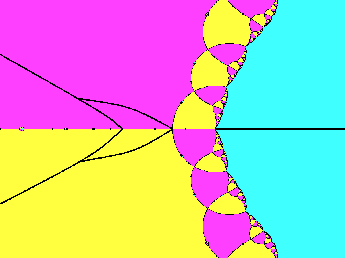
Figure 5. Julia set of $N_{\lambda}$ with $\lambda=0.1i$. The Head’s angle is $\alpha$.

Definition 5.1.

For $\lambda\in\Omega_{0}\cup\{\sqrt{3}i/2\}$, the Head’s angle $\boldsymbol{h}(\lambda)$ of $N_{\lambda}$ is defined as the infimum of the angles in $\Theta_{\lambda}$ (as a subset of $(0,1]$).

Fact 5.2.

When $\lambda=\sqrt{3}i/2$, the Head’s angle $\boldsymbol{h}(\lambda)=1/2$.

Proof.

In this case, $N_{\lambda}(0)=\infty$. In the dynamical plane, it is known from Fact 4.5 that the internal rays $R_{\lambda}^{1}(1/2)$ and $R_{\lambda}^{2}(1/2)$ land at the critical point $0$. This implies that $\boldsymbol{h}(\sqrt{3}i/2)\leq 1/2$. One should also observe by the local behavior of $N_{\lambda}$ near the critical point $0$ that $R_{\lambda}^{1}(1/2),T_{\lambda}^{2},T_{\lambda}^{1},R_{\lambda}^{2}(1/2)$ attach $0$ in positive cyclic order, where $T_{\lambda}^{\varepsilon}$ is the component of $N_{\lambda}^{-1}(B_{\lambda}^{\varepsilon})$ other that $B_{\lambda}^{\varepsilon}$. To prove that $\boldsymbol{h}(\lambda)=1/2$, it suffices to show

Claim: For any $\theta\in[1/2,1)\cap\Theta_{\lambda}$, we have $\theta/2\notin\Theta_{\lambda}$.

Figure 6. Julia set of $N_{\lambda}$ with $\lambda=\sqrt{3}i/2$. The internal angles are labeled beside the corresponding internal rays.

The claim implies that $(0,1/2)\cap\Theta_{\lambda}=\emptyset$. In what follows, we prove this claim. By looking at the $N_{\lambda}$-preimage of the components of

$$\mathbb{\widehat{C}}\setminus\Big{(}\overline{{R}_{\lambda}^{1}}(0)\cup\overline{{R}_{\lambda}^{1}}(\theta)\cup\overline{{R}_{\lambda}^{2}}(0)\cup\overline{{R}_{\lambda}^{2}}(1-\theta)\Big{)},$$

we see that $R_{\lambda}^{1}(\theta/2)$ attaches the internal ray in $T_{\lambda}^{2}$ of angle $1-\theta$, and $R_{\lambda}^{2}(1-\theta/2)$ attaches the internal ray in $T_{\lambda}^{1}$ of angle $\theta$. Therefore the internal rays $R_{\lambda}^{1}(\theta/2)$ and $R_{\lambda}^{2}(1-\theta/2)$ can not land at the same point. This means $\theta/2\notin\Theta_{\lambda}$, completing the proof. ∎

Proposition 5.3.

For any $\lambda\in\Omega_{0}$, the Head’s angle $\boldsymbol{h}(\lambda)$ satisfies:

1. $0<\boldsymbol{h}(\lambda)<\frac{1}{2}$ and $\boldsymbol{h}(\lambda)\in\Theta_{\lambda}$.

2. $\theta\in\Theta_{\lambda}$ if and only if $2^{n}\theta\in[\boldsymbol{h}(\lambda),1]$ for all $n\geq 0$. This implies that $\Theta_{\lambda}=\bigcap_{k\geq 0}\tau^{-k}([\boldsymbol{h}(\lambda),1])$ is totally disconnected .

Proof.

For the proof, see [Ro08, Lemma 3.15 and Corollary 7.11]. ∎

5.2. The set $\Xi$

It’s known from Proposition 5.3 that for any $\lambda\in\Omega_{0}$, the Head’s angle $\boldsymbol{h}(\lambda)$ of $N_{\lambda}$ is contained in the set $\Xi$, here we recall the definition

$$\Xi=\{\theta\in(0,1/2];2^{k}\theta\in[\theta,1]\ ({\rm mod}\ \mathbb{Z})\text{ for all }k\geq 0\}.$$

It’s clear that $1/2^{k}\in\Xi$, for all $k\geq 1$.

Lemma 5.4 (Tan Lei [Tan]).

The set $\Xi$ satisfies the following properties:

1. The set $\Xi\cup\{0\}$ is closed, totally disconnected, perfect (without isolated points) and of $0$-Lebesgue measure.

2. Let $(\beta,\alpha)$ be a connected component of $(0,1/2)\setminus\Xi$, then $\alpha$ and $\beta$ are of the form

$$\alpha={p\over 2^{n}-1}\quad\text{ and }\quad\beta={p\over 2^{n}},\quad\text{ with }\quad n\geq 2.$$

3. If $\beta=p/2^{m}$ (resp. $\alpha=p/(2^{n}-1)$) is in $\Xi$, it is necessarily the infimum (resp. supremum) of a connected component $(\beta,\overline{\alpha})$ (resp. $(\overline{\beta},\alpha)$) of $(0,1/2)\setminus\Xi$, where $\overline{\alpha}=p/(2^{m}-1)$ (resp. $\overline{\beta}=p/2^{n}$).

Proof.

Points 1) and 3) correspond to Proposition 2.16 in [Tan]. Point 2) is exactly Lemma 2.24 in [Tan]. ∎

Recall that the sets $\Theta_{per},\Theta_{dya}$ in Section 1 are defined as follows

$$\Theta_{per}=\{t\in(0,1/2];2^{k}t=t\ ({\rm mod}\ \mathbb{Z})\text{ for some }k\geq 1\},$$

$$\Theta_{dya}=\{t\in(0,1/2];2^{k}t=1\ ({\rm mod}\ \mathbb{Z})\text{ for some }k\geq 1\}.$$

The following fact is easy to verify

Fact 5.5.

Let $\partial(\Xi)$ be the collection of the endpoints of all interval components of $(0,1/2)\setminus\Xi$, together with $1/2$. Then

$$\partial(\Xi)=(\Xi\cap\Theta_{per})\cup(\Xi\cap\Theta_{dya}).$$

By definition and Proposition 5.3, we know that the Head’s angle $\boldsymbol{h}(\lambda)$ is the minimum of the angles in the set $\Theta_{\lambda}$. The following result will tell us in which case $\boldsymbol{h}(\lambda)$ is an accumulation point of $\Theta_{\lambda}$.

Proposition 5.6.

Let $\alpha\in\Xi$, we define a set $C_{\alpha}$ by

$$C_{\alpha}=\bigcap_{k\geq 0}\tau^{-k}([\alpha,1]).$$

1. If $\alpha$ is dyadic, then $\alpha$ is an isolated point of $C_{\alpha}$;

2. If $\alpha$ is non-dyadic, then $\alpha$ is an accumulation point of the non-dyadic (or dyadic) rational numbers in $C_{\alpha}$.

Proof.

If $\alpha$ is dyadic, then there is a smallest integer $k\geq 1$ such that $2^{k}\alpha=1$. Take $\delta=\alpha/2^{k+1}$, we claim that $(\alpha,\alpha+\delta)\cap C_{\alpha}=\emptyset$. This is because $2^{k}(\alpha,\alpha+\delta)=(0,\alpha/2)({\rm mod}\ \mathbb{Z})$ which has no intersection with $[\alpha,1]$. Therefore $\alpha$ is an isolated point of $C_{\alpha}$.

To prove the second statement, note that $[\alpha,1)\cap\Xi\subset C_{\alpha}$. Because $\alpha$ is non-dyadic and by Lemma 5.4, we can find a decreasing sequence of rationals $\{r_{n}\}\subset(\Xi\cap\Theta_{per})\cap C_{\alpha}$ (or $(\Xi\cap\Theta_{dya})\cap C_{\alpha}$) with limit $\alpha$, where each $r_{n}$ takes the form $\frac{p_{n}}{2^{q_{n}}-1}$ (or $\frac{p_{n}}{2^{q_{n}}}$). This completes the proof. ∎

5.3. Maps with the same Head’s angle

There are two natural questions:

Q1: Which angles $\theta\in\Xi$ arise as Head’s angles for cubic Newton maps?

Q2: Which cubic Newton maps have the same Head’s angle?

These questions both have complete answers, see Theorems 1.3 and 1.4, whose proofs are given in Section 11. But for the moment, with what we have known in hand, we only consider (special cases of) the second question Q2. For some special cases of $\theta\in\Xi$, Tan Lei posed the following conjecture [Tan, p.231 Conjecture]:

Conjecture 5.7.

Given any component $(\beta,\alpha)$ of $(0,1/2)\setminus\Xi$, there is a unique connected component of $\Omega-\overline{\mathcal{H}_{0}^{1}\cup\mathcal{H}_{0}^{2}}$ such that the maps in the closure of this component are precisely the maps with Head’s angle $\beta$ or $\alpha$.

To confirm this conjecture (a tiny mistake of the conjecture is corrected in Corollary 5.10), we establish the following crucial result.

Theorem 5.8.

Let $(\beta,\alpha)$ be a connected component of $(0,1/2)\setminus\Xi$, and let $\theta=\beta$ or $\alpha$.

1. The parameter rays $\mathcal{R}_{0}^{1}(\theta)$ and $\mathcal{R}_{0}^{2}(1-\theta)$ land at the same point, say $\lambda_{\theta}$.

2. Let $\mathcal{U}_{\theta}$ be the bounded component of

$$\mathbb{C}\setminus\Big{(}\Big{[}-\frac{1}{2},\frac{1}{2}\Big{]}\cup\overline{\mathcal{R}_{0}^{1}}(\theta)\cup\overline{\mathcal{R}_{0}^{2}}(1-\theta)\Big{)},$$

then $\mathcal{U}_{\theta}\cup\{\lambda_{\theta}\}$ consists of the parameters $\lambda\in\Omega$ for which, in the dynamical plane, the internal rays ${R}_{\lambda}^{1}(\theta)$ and ${R}_{\lambda}^{2}(1-\theta)$ land at the same point $x_{\lambda}$. Moreover, this point $x_{\lambda}$ is

• 0, if $\lambda=\lambda_{\beta}$;

• a parabolic periodic point, if $\lambda=\lambda_{\alpha}$;

• pre-repelling point, whose orbit does not contain the critical point $0$, if $\lambda\in\mathcal{U}_{\theta}$.

In particular, $\lambda_{\alpha}\neq\lambda_{\beta}$.

See Figure 7 and Figure 8.

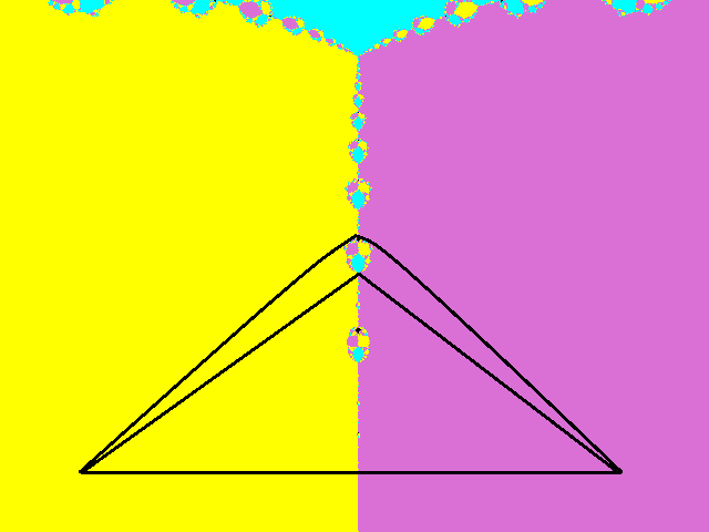
Figure 7. Parameter rays landing at the same point (left) and the local picture (right).

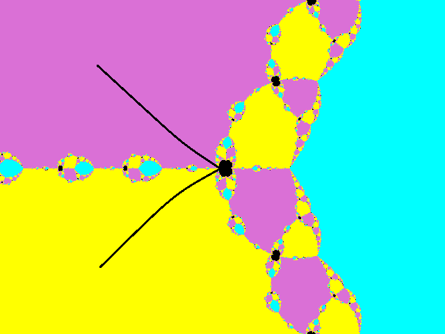
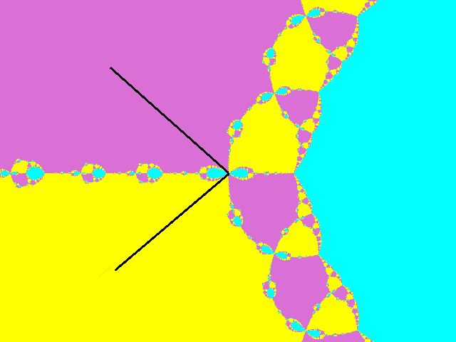
Figure 8. Left: the dynamical plane of $N_{\lambda_{\alpha}}$, the Head’s angle is $\alpha$ and the ray $R_{\lambda_{\alpha}}^{1}(\alpha)$ lands at a parabolic point. Right: the dynamical plane of $N_{\lambda_{\beta}}$, the Head’s angle is $\beta$ and the ray $R_{\lambda_{\beta}}^{1}(\beta)$ lands at the critical point $0$.

We remark that the theorem is also true for $\theta=1/2$, which is not included in the statement. Before the proof, we need a lemma:

Lemma 5.9.

Let $n\geq 1$ and $\theta=p/2^{n}\in\Xi$. Then there exists a parameter $\lambda$ in $\Omega_{0}$ with $\boldsymbol{h}(\lambda)=\theta$.

Proof.

For $n=1$, it suffices to take the map $N_{\lambda}$ with $\lambda=i\sqrt{3}/2$ (see Fact 5.2). For $n>1$, let $\lambda$ be the landing point of the ray $\mathcal{R}_{0}^{1}(p/2^{n})$. Since the ray $R^{1}_{\lambda}(p/2^{n})$ lands at a pre-repelling point, it lands in fact at the critical point $0$ (see the proof of Lemma 4.6).

Let $w_{2}=w_{2}(\lambda)$ denote the first pre-image of $b_{2}(\lambda)$, $U_{\lambda}$ be the Fatou component containing $w_{2}$. We denote by $\gamma$ the largest $t\in(0,1/2)$ such that the rays $R^{1}_{\lambda}(t)$ and $(N_{\lambda}|_{U_{\lambda}})^{-1}(R^{2}_{\lambda}(1-2t))$ land at the same point. It is clear that $2\gamma\in\Theta_{\lambda}$. By the location of the critical point $0$ [Ro08, Lemma 3.14], we have $\gamma\leq\theta\leq\boldsymbol{h}(\lambda)$. Let’s denote by $\theta^{\prime}$ the last iteration of $\theta$ in $[\gamma,\boldsymbol{h}(\lambda)]$ (it can happen that $\gamma=\boldsymbol{h}(\lambda)$). Since $\tau^{j}(\theta^{\prime})\geq\boldsymbol{h}(\lambda)$ for all $j\geq 1$,  $\tau(\theta^{\prime})\in C_{\boldsymbol{h}(\lambda)}=\Theta_{\lambda}$. There are three possibilities:

Case 1: $\theta^{\prime}\in(\gamma,\boldsymbol{h}(\lambda))$. Therefore, $\tau(\theta^{\prime})\in\Theta_{\lambda}\cap(\tau(\gamma),\tau(\boldsymbol{h}(\lambda)))$. But this set is empty by the definition of $\gamma$.

Case 2: $\theta^{\prime}=\boldsymbol{h}(\lambda)$. By looking at the successive $N_{\lambda}$-preimages of $\overline{R_{\lambda}^{1}}(\theta^{\prime})\cup\overline{R_{\lambda}^{2}}(1-\theta^{\prime})$, we see that $\theta=\theta^{\prime}$ implying $\boldsymbol{h}(\lambda)=\theta$.

Case 3: $\theta^{\prime}=\gamma$. This implies $2\theta^{\prime}\in\Theta_{\lambda}$, namely $R_{\lambda}^{1}(2\theta^{\prime})$ and $R_{\lambda}^{2}(1-2\theta^{\prime})$ land at the same point. By looking at the $N_{\lambda}$-preimage of $\overline{R_{\lambda}^{1}}(2\theta^{\prime})\cup\overline{R_{\lambda}^{2}}(1-2\theta^{\prime})$, we see that $R_{\lambda}^{1}(\theta^{\prime})$ and $R_{\lambda}^{2}(1-\theta^{\prime})$ both land at the critical point $0$, meaning that $\boldsymbol{h}(\lambda)=\gamma=\theta=\theta^{\prime}$. ∎

Proof.

: Let $\mathcal{Y}_{\theta}$ be the set of parameters $\lambda\in\Omega$ for which the following conditions are satisfied :

• the sets $R_{\lambda}^{1}(\theta)$ and $R_{\lambda}^{2}(1-\theta)$ are internal rays;

• these two rays land at the same point $x=x(\lambda)$ ;

• the point $x$ is an eventually repelling periodic point.

We then define $\mathcal{X}_{\theta}$ as the set of parameters of $\mathcal{Y}_{\theta}$ for which the orbit of the landing point $x$ does not contain the critical point $0$.

Claim a .

If $\theta,\theta^{\prime}$ are in $\Xi\cap\mathbb{Q}$ and if $\theta<\theta^{\prime}$, then

$$\mathcal{X}_{\theta}\subset\mathcal{Y}_{\theta}\subset\mathcal{X}_{\theta^{\prime}}\subset\mathcal{Y}_{\theta^{\prime}}\,.$$

Proof.

(of Claim a) Indeed, if $\lambda$ is in $\mathcal{Y}_{\theta}$, since $R_{\lambda}^{1}(\theta)$ and $R_{\lambda}^{2}(1-\theta)$ land at the same point, the critical point $0$ are in the closure of $V_{1,2}(0,\theta)$ (see [Ro08, Lemma 3.14]), where $V_{1,2}(0,\theta)$ is the component of $\mathbb{\widehat{C}}\setminus\big{(}\overline{{R}_{\lambda}^{1}}(0)\cup\overline{{R}_{\lambda}^{2}}(0)\cup\overline{{R}_{\lambda}^{1}}(\theta)\cup\overline{{R}_{\lambda}^{2}}(1-\theta)\big{)}$ containing the set ${R}_{\lambda}^{1}(\theta/2)$. Since $\theta^{\prime}\in\Xi$, for every $i\geq 0$,  $\tau^{i}(\theta^{\prime})$ belong to $[\theta^{\prime},1]$, implying that the orbits of the two sets $R_{\lambda}^{1}\bigl{(}\theta^{\prime}\bigr{)}$ and $R_{\lambda}^{2}\bigl{(}1-\theta^{\prime}\bigr{)}$ are always in $\mathbb{\widehat{C}}\setminus\overline{V_{1,2}(0,\theta)}$. Therefore $R_{\lambda}^{1}\bigl{(}\theta^{\prime}\bigr{)},R_{\lambda}^{2}\bigl{(}1-\theta^{\prime}\bigr{)}$ are internal rays.

Let $U_{k}$ be the component of $N_{\lambda}^{-k}(\mathbb{\widehat{C}}\setminus\overline{V_{1,2}(0,\theta)})$ containing $R_{\lambda}^{1}\bigl{(}\theta^{\prime}\bigr{)}\cup R_{\lambda}^{2}\bigl{(}1-\theta^{\prime}\bigr{)}$. Then $V_{k}=U_{0}\cap U_{1}\cap\cdots\cap U_{k},\ k\in\mathbb{N}$ is a shrinking sequence of disks, each bounded by four internal rays. It’s easy to verify that

$$\overline{R_{\lambda}^{1}}\bigl{(}\theta^{\prime}\bigr{)}\cup\overline{R_{\lambda}^{2}}\bigl{(}1-\theta^{\prime}\bigr{)}=\bigcap_{k}\overline{V_{k}}.$$

This implies that the internal rays $R_{\lambda}^{1}\bigl{(}\theta^{\prime}\bigr{)},R_{\lambda}^{2}\bigl{(}1-\theta^{\prime}\bigr{)}$ land at the same point in $\mathbb{\widehat{C}}\setminus\overline{V_{1,2}(0,\theta)}$. Moreover, this point is necessarily pre-repelling because of the location of the critical point (see [Ro08, Lemma 3.14]), and also in $\mathcal{X}_{\theta^{\prime}}$ since $R_{\lambda}^{1}(\tau^{i}(\theta^{\prime}))$ stays in $\mathbb{\widehat{C}}\setminus\overline{V_{1,2}(0,\theta)}$ for $i\geq 0$. ∎

From Lemma 5.4, if $(\beta,\alpha)$ is a connected component of $(0,1/2)\setminus\Xi$, its bounds can be written as $\alpha=p/(2^{k}-1)$ and $\beta=p/2^{k}$.

We now prove by induction on $k$, the following property

$$\mathfrak{P}(k) \theta\in\Bigl{\{}\alpha={p\over 2^{k}-1},\beta={p\over 2^{k}}\Bigr{\}}\cap\Xi,$$ : for all

$$\left\{\vphantom{\begin{aligned} &\mathcal{X}_{\theta}=\mathcal{U}_{\theta}\text{ \ and}\\ &\mathcal{R}_{\mathcal{H}_{-}}(2\theta),\ \ \mathcal{R}_{\mathcal{H}_{+}}(-2\theta)\text{ \ land at the same point.}\end{aligned}}\right. \begin{aligned} &\mathcal{X}_{\theta}=\mathcal{U}_{\theta}\text{ \ and}\\ &\mathcal{R}_{0}^{1}(\theta),\ \mathcal{R}_{0}^{2}(1-\theta)\text{ \ land at the same point.}\end{aligned}$$

$\bullet$ Proof of $\mathfrak{P}(1)$ :  In this case, we need show that $\mathcal{X}_{1/2}=\Omega$. By Fact 4.5, for all $\lambda\in\Omega$, the sets $R_{\lambda}^{1}(1/2)$ and $R_{\lambda}^{2}(1/2)$ are internal rays and land at a pre-image of infinity, which is a repelling fixed point. Thus, $\mathcal{Y}_{1/2}=\Omega$. On the other side, if $\lambda$ is in $\Omega$, it is not on $\overline{\mathcal{R}_{0}^{1}}(1/2)$. Thus, $R_{\lambda}^{1}(1/2)$ does not land at the critical point $0$. So, $\lambda$ is in $\mathcal{X}_{1/2}$, hence $\mathcal{X}_{1/2}=\Omega$. Finally, $\mathfrak{P}(1)$ is verified since the rays $\mathcal{R}_{0}^{1}(1/2)$ and $\mathcal{R}_{0}^{2}(1/2)$ both land at $i\sqrt{3}/2$ and it follows that $\Omega=\mathcal{U}_{1/2}$.

$\bullet$ Idea of the proof of $\mathfrak{P}(k)$ :  Thanks to the Claim, we can proof at first that $\mathcal{X}_{\theta}$ is included in an open set of the form $\mathcal{U}_{\beta^{\prime}}$, where $\beta^{\prime}$ verifies one of the properties $\mathfrak{P}(i)$, ${1\leq i\leq k-1}$. Then we prove that $\mathcal{X}_{\theta}$ is an open set whose boundary is contained in $\overline{\mathcal{R}_{0}^{1}}(\theta)\cup\overline{\mathcal{R}_{0}^{2}}(1-\theta)$ and a finite number of points. It follows then by a topology argument (see below) that $\mathcal{X}_{\theta}$ and $\mathcal{U}_{\theta}$ differ by a finite set, which is shown to be empty in the final step.

$\bullet$ Proof of $\mathfrak{P}(k)$ :  Define

$$\mathcal{E}_{k}=\left\{{q\over 2^{r}}\in\Xi\mid{q\over 2^{r}}>\alpha,\text{ and }r<k\right\}\,.$$

Every element of $\mathcal{E}_{k}$ is the infimum of a connected component $(q/2^{r},q/(2^{r}-1))$ of $(0,1/2)\setminus\Xi$. Denote by $\beta^{\prime}$ the minimum of $\mathcal{E}_{k}$.

Claim b .

The sets $\mathcal{X}_{\alpha}$ and $\mathcal{X}_{\beta}$ are open and non empty.

Proof.

If $\beta_{0}$ is a dyadic element of $\Xi$, Lemma 5.9 implies that $\mathcal{Y}_{\beta_{0}}$ is non empty. By Claim a, for any $\beta_{0}<\beta$, we have $\mathcal{Y}_{\beta_{0}}\subset\mathcal{X}_{\beta}\subset\mathcal{X}_{\alpha}$. This allows us to conclude that $\mathcal{X}_{\beta}$ and $\mathcal{X}_{\alpha}$ are non empty.

By definition, for $\lambda_{0}\in\mathcal{X}_{\theta}$, $\theta\in\{\alpha,\beta\}$, the landing point $z(\lambda_{0})$ of the rays $R^{1}_{\lambda_{0}}(\theta),R^{2}_{\lambda_{0}}(1-\theta)$ is pre-repelling, and does not contain the critical point in its orbit. Thus, $z(\lambda_{0})$ posses a neighborhood in which $N_{\lambda}$, for $\lambda$ in a neighborhood of $\lambda_{0}$, has a unique pre-repelling point $z(\lambda)$ (Fact 4.3). Moreover, the orbit of $z(\lambda)$ does not contain the critical point. This shows that $\lambda\in\mathcal{X}_{\theta}$. ∎

Claim c .

For $\theta\in\{\alpha,\beta\}$, the intersection $\partial\mathcal{X}_{\theta}\cap\Omega$ is contained in

$$\bigcup_{i\in I}\mathcal{R}_{0}^{1}\bigl{(}\tau^{i}(\theta)\bigr{)}\cup\mathcal{R}_{0}^{2}\bigl{(}1-\tau^{i}(\theta)\bigr{)}\cup\mathcal{F}_{\theta}$$

where $\mathcal{F}_{\theta}$ is a finite set of points and $I=\{i\in\{0,\dots,k-1\}\mid\tau^{i}(\theta)\in[0,1/2]\}$. Moreover, if $\lambda\in\mathcal{F}_{\theta}$ and if $\theta=\beta$ (resp. if $\theta=\alpha$), one of the rays $R^{1}_{\lambda}(\theta),R^{2}_{\lambda}(1-\theta)$ converges to the critical point $0$, whose orbit contains $\infty$ (resp. to a parabolic periodic point).

Proof.

Indeed, take $\lambda\in\partial\mathcal{X}_{\theta}\cap\Omega$. Since $\lambda$ is not in $\mathcal{X}_{\theta}$, one of the following cases arises:

• One of the sets $R^{1}_{\lambda}(\theta)$, $R^{2}_{\lambda}(1-\theta)$ bifurcates. It means that one of the sets $R^{1}_{\lambda}(\tau^{i}(\theta))$, $R_{\lambda}^{2}(1-\tau^{i}(\theta))$ with $0\leq i\leq k-1$, contains the critical point $0$, in particular $\tau^{i}(\theta)$ is in $[0,1/2]$. The parameter $\lambda$ then belongs to $\mathcal{R}_{0}^{1}\bigl{(}\tau^{i}(\theta)\bigr{)}$ or to $\mathcal{R}_{0}^{2}\bigl{(}1-\tau^{i}(\theta)\bigr{)}$.

• The sets $R^{1}_{\lambda}(\theta)$, $R^{2}_{\lambda}(1-\theta)$ are internal rays and one of them converges to a pre-periodic point whose orbit contains the critical point $0$. Necessarily, $\theta=\beta$ and the parameter $\lambda$ is a solution of one of the equations $N_{\lambda}^{i+1}(0)=N^{i}_{\lambda}(0)$,  $i\leq k$. This gives a finite number of values of $\lambda$.

• The sets $R^{1}_{\lambda}(\theta)$, $R^{2}_{\lambda}(1-\theta)$ are internal rays and one of them converges to a pre-periodic point $x$, not pre-repelling. In this case $\theta=\alpha$, and point $x$ is necessarily parabolic. Then, the system

  $$\left\{\begin{aligned} N^{k}_{\lambda}(x)&=x\\ (N^{k}_{\lambda})^{\prime}(x)&=1\end{aligned}\right.$$

  has a solution. So $\lambda$ belongs to a finite set. ∎

Claim d .

For $\theta\in\{\alpha,\beta\}$, the set $\mathcal{X}_{\theta}$ is contained in $\mathcal{U}_{\beta^{\prime}}$ and the intersection $\partial\mathcal{X}_{\theta}\cap\mathcal{U}_{\beta^{\prime}}$ is included in

$$\mathcal{R}_{0}^{1}\bigl{(}\theta\bigr{)}\cup\mathcal{R}_{0}^{2}\bigl{(}1-\theta\bigr{)}\cup\mathcal{F}_{\theta}\,.$$

Proof.

The inclusion $\mathcal{X}_{\theta}\subset\mathcal{X}_{\theta^{\prime}}=\mathcal{U}_{\beta^{\prime}}$ follows from the induction hypothesis on $\beta^{\prime}$ and Claim a.

By Claim c, it is enough to prove that

$$\{\tau^{i}(\theta)\in[0,1/2];0\leq i\leq k-1\}\cap(0,\beta^{\prime})=\{\theta\}.$$

For $\theta=\beta$, let $i$ be the largest integer such that $\tau^{i}(\beta)\in(0,\beta^{\prime})$. Necessarily, $\tau^{i}(\beta)\in\Xi$, because $\tau^{i+k}(\beta)\geq\beta^{\prime}>\tau^{i}(\beta)$ for all $k\geq 0$. Moreover, if $i>0$, then $\tau^{i}(\beta)\in\mathcal{E}_{k}$ because $\tau^{i}(\beta)>\alpha$. But this contradicts the minimality of $\beta^{\prime}$, so $i=0$.

For $\theta=\alpha$ and $1\leq i\leq k-1$, the fact that $(\tau^{i}(\beta),\tau^{i}(\alpha))$ is an interval implying that $\beta^{\prime}\leq\tau^{i}(\beta)<\tau^{i}(\alpha)$. ∎

Claim e .

The open sets $\mathcal{U}_{\beta^{\prime}}\setminus\overline{\mathcal{X}}_{\alpha}$ and $\mathcal{U}_{\beta^{\prime}}\setminus\overline{\mathcal{X}}_{\beta}$ are non empty.

Proof.

Indeed, it is known from Lemma 5.4 that $\Xi\cup\{0\}$ has no isolated points and since $\alpha$ is the supremum of the connected component $(\beta,\alpha)$ of $(0,1/2)\setminus\Xi$, the interval $(\alpha,\beta^{\prime})$ contains at least a connected component of the open set $(0,1/2)\setminus\Xi$. We denote by $\beta_{1}$ its infimum. By Lemma 5.9, there is a parameter $\lambda_{1}$ with $\boldsymbol{h}(\lambda_{1})=\beta_{1}$, and the ray $R_{\lambda_{1}}^{1}(\beta_{1})$ lands at the critical point $0$. Such $\lambda_{1}$ is in $\mathcal{Y}_{\beta_{1}}$, thus in $\mathcal{X}_{\beta^{\prime}}=\mathcal{U}_{\beta^{\prime}}$ (by induction). It’s clear that $\lambda_{1}\notin\mathcal{X}_{\alpha}$. If $\lambda_{1}\in\partial\mathcal{X}_{\alpha}\cap\mathcal{U}_{\beta^{\prime}}$, then by Claim d, either it is on $\mathcal{R}_{0}^{1}(\alpha)\cup\mathcal{R}_{0}^{2}(1-\alpha)$, or $N_{\lambda_{1}}$ has a parabolic point (by the proof of Claim c). But, by construction of $N_{\lambda_{1}}$, this is impossible. In conclusion, $\lambda_{1}$ is in $\mathcal{U}_{\beta^{\prime}}\setminus\overline{\mathcal{X}}_{\alpha}\subset\mathcal{U}_{\beta^{\prime}}\setminus\overline{\mathcal{X}}_{\beta}$. ∎

We finish the proof of $\mathfrak{P}(k)$.  By the hypothesis of induction, the open set $\mathcal{X}_{\beta^{\prime}}=\mathcal{U}_{\beta^{\prime}}$ is a disk of $\widehat{\mathbb{C}}$. The set $\mathcal{X}_{\theta}$ is included in $\mathcal{U}_{\beta^{\prime}}$ from Claim a.

Define two closed arcs $\gamma_{1}:[0,1]\rightarrow\overline{\mathcal{R}_{0}^{1}}(\theta)$ and $\gamma_{2}:[0,1]\rightarrow\overline{\mathcal{R}_{0}^{2}}(1-\theta)$ by

$$\gamma_{1}(t)=(\Phi_{0}^{1})^{-1}(te^{2\pi i\theta}),\ \gamma_{2}(t)=(\Phi_{0}^{2})^{-1}(te^{2\pi i(1-\theta)}).$$

The two open sets $\mathcal{X}_{\theta},\mathcal{U}_{\beta^{\prime}}$ and the arcs $\gamma_{1},\gamma_{2}$ satisfy that

• semi-open arcs $\gamma_{\varepsilon}((0,1])$, $\varepsilon=1,2$, are contained in the disk  $\mathcal{U}_{\beta^{\prime}}$;

• $\gamma_{\varepsilon}(0)\in\partial\mathcal{U}_{\beta^{\prime}}$, $\varepsilon=1,2$ ;

• $\partial\mathcal{X}_{\theta}\cap\mathcal{U}_{\beta^{\prime}}$ is included in the union of a finite set of points and the semi-open arcs $\gamma_{\varepsilon}((0,1])$, $\varepsilon=1,2$ ;

• $\mathcal{U}_{\beta^{\prime}}\setminus\overline{\mathcal{X}_{\theta}}\neq\emptyset$.

In the following, we claim that $\gamma_{1}(1)=\gamma_{2}(1)$, which means that $\mathcal{R}_{0}^{1}(\theta)$ and $\mathcal{R}_{0}^{2}(1-\theta)$ land at the same point. To this end, let $F$ be the finite set so that $\partial\mathcal{X}_{\theta}\cap\mathcal{U}_{\beta^{\prime}}\subset\gamma_{1}((0,1])\cup\gamma_{2}((0,1])\cup F$. If $\gamma_{1}(1)\neq\gamma_{2}(1)$, let’s consider the open set $U=\mathcal{U}_{\beta^{\prime}}\setminus(\gamma_{1}((0,1])\cup\gamma_{2}((0,1])\cup F)$. It’s clear that $\mathcal{X}_{\theta}\subset U$ and $\partial\mathcal{X}_{\theta}\cap U=\emptyset$. This implies that $U=\mathcal{X}_{\theta}$ and $\overline{\mathcal{X}_{\theta}}=\overline{U}\supset\mathcal{U}_{\beta^{\prime}}$, contradicting the fact $\mathcal{U}_{\beta^{\prime}}\setminus\overline{\mathcal{X}_{\theta}}\neq\emptyset$. This proves the claim.

The open arc $\gamma_{1}((0,1])\cup\gamma_{2}((0,1])$ then separates the $\mathcal{U}_{\beta^{\prime}}$ into two components: $\mathcal{U}_{\theta}$ and $\mathcal{U}_{\beta^{\prime}}\setminus\overline{\mathcal{U}_{\theta}}$.

By Claim e, we know that the parameter $\lambda_{1}$ of Head angle $\beta_{1}(>\alpha)$ is contained in $\mathcal{U}_{\beta^{\prime}}\setminus\overline{\mathcal{X}_{\theta}}$. Note that $\beta_{1}\notin\mathcal{U}_{\beta^{\prime}}\setminus\overline{\mathcal{U}_{\theta}}$. We have that

$$\mathcal{U}_{\theta}=\mathcal{X}_{\theta}\cup\mathcal{F}_{\theta},$$

where $\mathcal{F}_{\theta}$ is a finite set in $\mathcal{U}_{\theta}$. To obtain $\mathfrak{P}(k)$, we will show in the following that $\mathcal{F}_{\theta}=\emptyset$. In fact, if $\lambda_{0}\in\mathcal{F}_{\theta}\neq\emptyset$, then there are two possibilities:

If $\theta=\beta$, then one of the rays $R^{1}_{\lambda_{0}}(\tau^{i}(\theta)),R^{2}_{\lambda_{0}}(1-\tau^{i}(\theta))$, $0\leq i\leq k-1$, converges to the critical point $0$ (Claim c). It follows that the corresponding angle $\tau^{i}(\theta)$ belongs to $[0,1/2]$ and $\lambda_{0}$ is the landing point of the ray $\mathcal{R}_{0}^{1}(\tau^{i}(\theta))$ or $\mathcal{R}_{0}^{2}(1-\tau^{i}(\theta))$  (Lemma 4.7). But, since $\tau^{i}(\theta)\geq\theta$ (because $\theta\in\Xi$), none of these rays is in $\mathcal{U}_{\theta}$.

If $\theta=\alpha$, then one of the rays $R^{1}_{\lambda_{0}}(\theta),R^{2}_{\lambda_{0}}(1-\theta)$ converges to a parabolic point of period $k$ (Claim c). Let us take a disk $\Delta\subset\mathcal{U}_{\alpha}$ such that $\Delta\cap\mathcal{F}_{\theta}=\{\lambda_{0}\}$. For $\lambda\in\Delta\setminus\{\lambda_{0}\}$, the rays $R_{\lambda}^{1}(\theta),R_{\lambda}^{2}(1-\theta)$ converge to repelling $k$-periodic points which are stable and that we denote by $z_{1}(\lambda),z_{2}(\lambda)$. The functions

$$\rho_{\varepsilon}:\Delta\setminus\{\lambda_{0}\}\longrightarrow{\mathbb{C}}\setminus\mathbb{D},\quad\lambda\longmapsto\rho_{\varepsilon}(\lambda)=\bigl{(}N_{\lambda}^{k}\bigr{)}^{\prime}\bigl{(}z_{\varepsilon}(\lambda)\bigr{)},$$

are holomorphic functions and have an unessential singularity at $\lambda_{0}$. However, $|\rho_{\varepsilon}|$ reaches its maximum at $\lambda_{0}$, which is impossible.

This finishes the proof of the identity $\mathcal{U}_{\theta}=\mathcal{X}_{\theta}$ and so of $\mathfrak{P}(k)$.

To complete the proof of Theorem 5.8, it is enough to verify the following two claims.

Claim f .

Let $\mathcal{Z}_{\beta}$ be the set of parameters $\lambda\in\Omega$ for which $R^{1}_{\lambda}(\beta)$, $R^{2}_{\lambda}(1-\beta)$ are internal rays converging to the critical point $0$. Then

$$\mathcal{Y}_{\beta}\setminus\mathcal{X}_{\beta}=\mathcal{Z}_{\beta}=\bigl{\{}\lambda_{\beta}\bigr{\}}\,.$$

Proof.

The identity $\{\lambda_{\beta}\}=\mathcal{Z}_{\beta}$ comes from Lemma 4.7. On the other side, if $\lambda$ belongs to $\mathcal{Y}_{\beta}\setminus\mathcal{X}_{\beta}$, the rays $R^{1}_{\lambda}(\beta),R^{2}_{\lambda}(1-\beta)$ land at the same point whose orbit contains the critical point $0$. Since $0$ and the set ${R}_{\lambda}^{1}(\beta/2)$ are contained in the same connected component of $\mathbb{\widehat{C}}\setminus\big{(}\overline{{R}_{\lambda}^{1}}(0)\cup\overline{{R}_{\lambda}^{2}}(0)\cup\overline{{R}_{\lambda}^{1}}(\beta)\cup\overline{{R}_{\lambda}^{2}}(1-\beta)\big{)}$ and that $\tau^{k}(\beta)\in(\beta,1]$ for every $k>0$, we conclude that $R^{1}_{\lambda}(\beta)$ converges to $0$ and $\lambda$ thus belongs to $\mathcal{Z}_{\beta}$. The converse is clear. ∎

Claim g .

Let $\mathcal{Z}_{\alpha}$ be the set of parameters $\lambda\in\Omega$ for which $R^{1}_{\lambda}(\alpha)$, $R^{2}_{\lambda}(1-\alpha)$ are internal rays converging to the same parabolic point. Then

$$\mathcal{Z}_{\alpha}=\bigl{\{}\lambda_{\alpha}\}\,.$$

Proof.

Let $\beta_{n}$ be a sequence of dyadic elements of $\Xi$ converging to $\alpha$ and satisfying $\beta_{n}>\alpha$. We show now that

$$\mathcal{Z}_{\alpha}=\mathcal{Q}_{\alpha}\quad\text{ where }\quad\mathcal{Q}_{\alpha}=\bigcap_{n\geq 0}\Bigl{(}\overline{\mathcal{U}}_{\beta_{n}}\setminus\bigl{(}\mathcal{U}_{\alpha}\cup\mathcal{H}_{0}^{1}\cup\mathcal{H}_{0}^{2}\bigr{)}\Bigr{)}\,.$$

The conclusion then follows since it is clear that $\mathcal{Z}_{\alpha}$ is finite, $\mathcal{Q}_{\alpha}$ is connected and that $\lambda_{\alpha}$ belongs to $\mathcal{Q}_{\alpha}$.

If $\lambda\in\mathcal{Q}_{\alpha}$, for every $n\geq 0$, the rays $R^{1}_{\lambda}(\beta_{n}),R^{2}_{\lambda}(1-\beta_{n})$ land at the same point. By continuity, the rays $R^{1}_{\lambda}(\alpha),R^{2}_{\lambda}(1-\alpha)$ land also at a common point, say $x$. Since $x\in\partial B^{1}_{\lambda}$ which is a Jordan curve, it is not an irrational indifferent point. On the other side, $x$ is periodic and in the Julia set, so its orbit cannot contain the critical point. It follows that, $x$ is not repelling since $\lambda$ does not belong to $\mathcal{U}_{\alpha}$. Therefore, $x$ is parabolic and $\lambda\in\mathcal{Z}_{\alpha}$.

If $\lambda\in\mathcal{Z}_{\alpha}$, then $\boldsymbol{h}(\lambda)\leq\alpha$. Since $\tau^{k}(\beta_{n})\geq\beta_{n}>\alpha$ for every $k\geq 0$, the angle $\beta_{n}\in\Theta_{\lambda}$ and the internal rays $R^{1}_{\lambda}(\beta_{n}),R^{2}_{\lambda}(-\beta_{n})$ thus land at the same pre-repelling point. It follows that $\lambda\in\mathcal{U}_{\beta_{n}}$ for every $n$. On the other side, $\lambda$ is not in $\mathcal{U}_{\alpha}\cup\mathcal{H}_{0}^{1}\cup\mathcal{H}_{0}^{2}$ since $\mathcal{U}_{\alpha}=\mathcal{X}_{\alpha}$ and $N_{\lambda}$ has a parabolic point. Therefore, $\lambda$ belongs to $\mathcal{Q}_{\alpha}$. ∎

The proof of Theorem 5.8 is completed. ∎

Recall that the fiber of $\boldsymbol{h}:\Omega_{0}\cup\{\sqrt{3}i/2\}\rightarrow\Xi$ over $\theta\in\Xi$ is defined by

$$\boldsymbol{h}^{-1}(\theta)=\{\lambda\in\Omega_{0}\cup\{\sqrt{3}i/2\};\boldsymbol{h}(\lambda)=\theta\}.$$

Corollary 5.10.

Let $(\beta,\alpha)$ be a connected component of $(0,1/2)\setminus\Xi$, then

$$\boldsymbol{h}^{-1}(\alpha)=\Omega_{0}\cap\big{(}\big{(}\mathcal{U}_{\alpha}\cup\{\lambda_{\alpha}\}\big{)}\setminus\big{(}\mathcal{U}_{\beta}\cup\{\lambda_{\beta}\}\big{)}\big{)},\ \boldsymbol{h}^{-1}(\beta)=\{\lambda_{\beta}\}.$$

5.4. Further properties of the Head’s angle

Theorem 5.8 allows us to give some further properties of the Head’s angles.

Given two numbers $\gamma_{1},\gamma_{2}\in\partial(\Xi)$ with $0<\gamma_{1}<\gamma_{2}<1/2$, define $V(\gamma_{1},\gamma_{2})$ to be the bounded component of

$$\mathbb{C}\setminus\Big{(}\overline{\mathcal{R}_{0}^{1}}(\gamma_{1})\cup\overline{\mathcal{R}_{0}^{2}}(1-\gamma_{1})\cup\overline{\mathcal{R}_{0}^{1}}(\gamma_{2})\cup\overline{\mathcal{R}_{0}^{2}}(1-\gamma_{2})\Big{)}.$$

Lemma 5.11.

For any $u\in V(\gamma_{1},\gamma_{2})\cap\Omega_{0}$, the Head’s angle of $N_{u}$ satisfies

$$\gamma_{1}\leq\boldsymbol{h}(u)\leq\gamma_{2}.$$

Proof.

By Theorem 5.8, we see that the two internal rays $R_{u}^{1}(\gamma_{2})$ and $R_{u}^{2}(1-\gamma_{2})$ land at the same point. So by the definition of the Head’s angle, we have $\boldsymbol{h}(u)\leq\gamma_{2}$. On the other hand, for any $\theta\in(0,\gamma_{1})$, again by Theorem 5.8, the internal rays $R_{u}^{1}(\theta)$ and $R_{u}^{2}(1-\theta)$ would never land at the same point. So we have $\boldsymbol{h}(u)\geq\gamma_{1}$. ∎

Lemma 5.12.

For any $\epsilon>0$ and any $\lambda\in\Omega_{0}$, there is a neighborhood $\mathcal{U}$ of $\lambda$, such that for all $u\in\mathcal{U}\cap\Omega_{0}$, the Head’s angle $\boldsymbol{h}(u)$ of $N_{u}$ satisfies

$$(1-\epsilon)\boldsymbol{h}(\lambda)\leq\boldsymbol{h}(u)\leq\frac{4}{3}\boldsymbol{h}(\lambda).$$

We remark that the right part of the above inequality cannot be improved to be $\boldsymbol{h}(u)\leq(1+\epsilon)\boldsymbol{h}(\lambda)$. This is because that the Head’s angle map $\boldsymbol{h}:\Omega_{0}\rightarrow\Xi$ is not continuous, following from Theorem 5.8.

Proof.

Recall that by Lemma 5.4, each number $s\in\Xi$ can be approximated by a sequence of numbers in $\partial(\Xi)$. Let $(\beta,\alpha)$ be a component of $(0,1/2)\setminus\Xi$. Fix a small number $\epsilon>0$. There are three possibilities:

If $\boldsymbol{h}(\lambda)=\alpha\in\partial(\Xi)$, then $\boldsymbol{h}(\lambda)$ can be approximated by a decreasing sequence of numbers in $\partial(\Xi)$. We may take $\gamma_{1}=\beta$ and $\gamma_{2}\in(\alpha,(1+\epsilon)\alpha)\cap\partial(\Xi)$. By Theorem 5.8, the set $V(\gamma_{1},\gamma_{2})$ contains a neighborhood $\mathcal{U}$ of $\lambda$. By Lemma 5.11, for any $u\in\mathcal{U}\cap\Omega_{0}$, we have $\boldsymbol{h}(\lambda)=\alpha\leq\boldsymbol{h}(u)\leq(1+\epsilon)\boldsymbol{h}(\lambda)$.

If $\boldsymbol{h}(\lambda)=\beta\in\partial(\Xi)$, then $\boldsymbol{h}(\lambda)$ can be approximated by an increasing sequence of numbers in $\partial(\Xi)$. Take $\gamma_{1}\in((1-\epsilon)\beta,\beta)\cap\partial(\Xi)$ and $\gamma_{2}=\alpha$. By Lemma 5.4, the number $\frac{\alpha}{\beta}$ takes the form $\frac{2^{p}}{2^{p}-1}$ for some $p\geq 2$. By Theorem 5.8, the set $V(\gamma_{1},\gamma_{2})$ contains a neighborhood $\mathcal{U}$ of $\lambda$. By Lemma 5.11, for any $u\in\mathcal{U}\cap\Omega_{0}$, we have

$$\boldsymbol{h}(\lambda)(1-\epsilon)\leq\boldsymbol{h}(u)\leq\alpha=\frac{\alpha}{\beta}\boldsymbol{h}(\lambda)=\frac{2^{p}}{2^{p}-1}\boldsymbol{h}(\lambda)\leq\frac{4}{3}\boldsymbol{h}(\lambda).$$

If $\boldsymbol{h}(\lambda)\in\Xi\setminus\partial(\Xi)$, then $\boldsymbol{h}(\lambda)$ can be approximated by two sequences of numbers in $\partial(\Xi)$ from both sides. We may choose two numbers $\gamma_{1},\gamma_{2}$ with

$$\gamma_{1}\in((1-\epsilon)\boldsymbol{h}(\lambda),\boldsymbol{h}(\lambda))\cap\partial(\Xi),\ \gamma_{2}\in(\boldsymbol{h}(\lambda),(1+\epsilon)\boldsymbol{h}(\lambda))\cap\partial(\Xi).$$

By Theorem 5.8, the set $V(\gamma_{1},\gamma_{2})$ contains a neighborhood $\mathcal{U}$ of $\lambda$. By Lemma 5.11, for any $u\in\mathcal{U}\cap\Omega_{0}$, we have $(1-\epsilon)\boldsymbol{h}(\lambda)\leq\boldsymbol{h}(u)\leq(1+\epsilon)\boldsymbol{h}(\lambda)$. ∎

The following result is a byproduct of the proof of Lemma 5.12:

Corollary 5.13.

The Head’s angle map $\boldsymbol{h}:\Omega_{0}\rightarrow\Xi$ is lower semi-continuous, that is, $\liminf_{u\rightarrow\lambda}\boldsymbol{h}(u)\geq\boldsymbol{h}(\lambda)$ for all $\lambda\in\Omega_{0}$. Moreover, $\lambda\in\Omega_{0}$ is a point of discontinuity if and only if $\boldsymbol{h}(\lambda)\in\Xi\cap\Theta_{dya}$.

6. Articulated rays

In this section, we first recall the construction of the articulated rays due to the first author [Ro08], which play a crucial role in the Yoccoz puzzle theory, then we show that the articulated rays satisfy the local stability property. This property is important in our later discussion.

6.1. The articulated ray

The articulated ray, analogous to the external ray in the polynomial case, is the starting point of the Yoccoz puzzle theory for the cubic Newton maps. It’s a kind of Jordan arc that intersects with the Julia set in countably many points. The construction of the articulated rays is due to Roesch [Ro08, Proposition 4.3]:

Theorem 6.1 (Roesch).

Let $\lambda\in\Omega_{0}$ and $\zeta\in\Theta_{\lambda}\cap(\boldsymbol{h}(\lambda),2\boldsymbol{h}(\lambda))$ be a non-dyadic rational angle. Then there exists a unique closed arc $L_{\lambda}(\zeta)$ stemming from $B_{\lambda}^{2}$ with angle $-\zeta/4$, converging to $y_{\lambda}$ which is the landing point of the internal ray $R_{\lambda}^{3}(1/7)$ and satisfying the 3-periodicity condition:

$$N_{\lambda}^{3}(L_{\lambda}(\zeta))=L_{\lambda}(\zeta)\cup\overline{R_{\lambda}^{1}}(\zeta)\cup\overline{R_{\lambda}^{2}}(-\zeta)\cup\overline{R_{\lambda}^{1}}(2\zeta)\cup\overline{R_{\lambda}^{2}}(-2\zeta).$$

Figure 9. The articulate ray $L_{\lambda}(\zeta)=L^{0}$, satisfying $N_{\lambda}(L^{0})=L^{1}$, $N_{\lambda}^{2}(L^{0})=L^{2}\cup\overline{R_{\lambda}^{1}}(\zeta)\cup\overline{R_{\lambda}^{2}}(-\zeta)$, and $N_{\lambda}^{3}(L^{0})=L^{0}\cup\overline{R_{\lambda}^{1}}(\zeta)\cup\overline{R_{\lambda}^{2}}(-\zeta)\cup\overline{R_{\lambda}^{1}}(2\zeta)\cup\overline{R_{\lambda}^{2}}(1-2\zeta)$. Note that four internal rays are also included in the picture.

The closed arc constructed in Theorem 6.1 is called the articulated ray. Theorem 6.1 is of fundamental importance when we study the dynamics of a single map. However, it is insufficient for our purpose when we are exploring the parameter plane because it does not tell us how the articulated ray moves as the parameter changes. We need to establish the local stability property (though it looks somewhat standard), saying that the articulated rays are also defined for the nearby maps, and what’s more, they move continuously in Hausdorff topology as the parameter varies. To this end, we will sketch the construction of the articulated rays following Roesch [Ro08], and we will see that the local stability property will follow immediately.

In our discussion, we fix some $\lambda\in\Omega_{0}=\Omega\setminus(\mathcal{H}_{0}^{1}\cup\mathcal{H}_{0}^{2})$. By Lemma 5.12, there is a neighborhood $\mathcal{U}\subset\Omega$ of $\lambda$ such that for all $u\in\mathcal{U}\cap\Omega_{0}$,

$$\Big{(}1-\frac{1}{10}\Big{)}\boldsymbol{h}(\lambda)\leq\boldsymbol{h}(u)\leq\Big{(}1+\frac{1}{3}\Big{)}\boldsymbol{h}(\lambda).$$

This implies that

$$H_{\mathcal{U}}:=\sup_{u\in\mathcal{U}\cap\Omega_{0}}\boldsymbol{h}(u)<\frac{3}{2}\inf_{u\in\mathcal{U}\cap\Omega_{0}}\boldsymbol{h}(u).$$

By shrinking $\mathcal{U}$ if necessary, we may assume that $H_{\mathcal{U}}<1/2$. By Lemma 5.4, we know that $\Xi\cup\{0\}$ is closed and perfect, therefore $H_{\mathcal{U}}\in\Xi$ and there is a non-dyadic rational number $\sigma\in\Xi\cap[H_{\mathcal{U}},1/2)$, equal to or sufficiently closed to $H_{\mathcal{U}}$, satisfying that

$$C_{\sigma}\bigcap\Big{[}\sigma,\frac{4}{3}\sigma\Big{]}\subset\bigcap_{u\in\mathcal{U}\cap\Omega_{0}}\Big{(}\Theta_{u}\cap(\boldsymbol{h}(u),2\boldsymbol{h}(u))\Big{)},\ \ \ (*)$$

here, recall that the sets $C_{\sigma},\Theta_{u}$ are defined by

$$C_{\sigma}=\bigcap_{k\geq 0}\tau^{-k}([\sigma,1]),\ \Theta_{u}=C_{\boldsymbol{h}(u)}=\bigcap_{k\geq 0}\tau^{-k}([\boldsymbol{h}(u),1]),$$

where $\tau$ is the doubling map on the unit circle, see Section 5.1.

By Proposition 5.6, there is a dyadic angle $\theta\in C_{\sigma}\bigcap(\sigma,\frac{4}{3}\sigma)$. By $(*)$ and Facts 4.3 and 4.4, for all $u\in\mathcal{U}$ (shrink $\mathcal{U}$ if necessary), the sets $R_{u}^{1}(\theta),R_{u}^{2}(1-\theta)$ are internal rays landing at same point $p_{u}$ which is pre-repelling (note that $N_{u}^{k}(p_{u})=\infty$ for some positive integer $k$), and their closures $\overline{R_{u}^{1}}(\theta),\overline{R_{u}^{2}}(1-\theta)$ move continuously with respect to $u\in\mathcal{U}$.

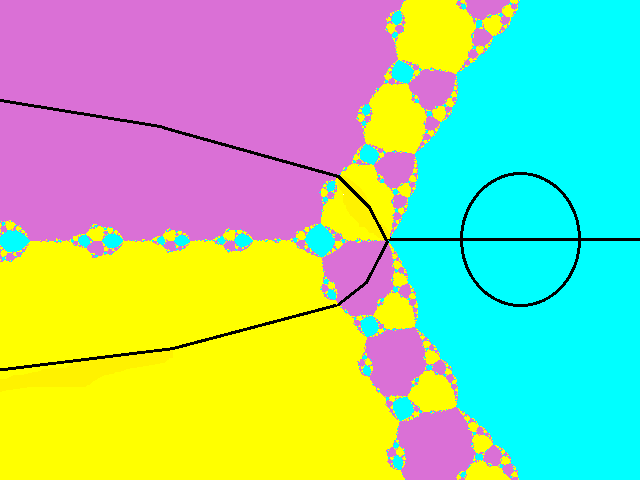
Figure 10. The domains $V_{u}$ (left) and $W_{u}^{\varepsilon}$ (right). Note that: the internal rays with angles $\zeta,\gamma=\boldsymbol{h}(u)(\geq\sigma)$ are included (left), a part of $N_{u}^{-1}(G)$ is not included (right).

For any $u\in\mathcal{U}$, we denote by $V_{u}$ the connected component of $\mathbb{\widehat{C}}\setminus G$ where

$$G=\overline{R_{u}^{1}}(0)\cup\overline{R_{u}^{2}}(0)\cup\overline{R_{u}^{1}}(\theta)\cup\overline{R^{2}_{u}}(1-\theta)\cup\overline{R_{u}^{3}}(0)\cup E_{u}^{3}(1/2)$$

(here $E_{u}^{3}(1/2)=(\phi_{u}^{3})^{-1}(\{|z|=1/2\})$ is the equipotential curve in $B_{u}^{3}$) which does not contain the critical value $N_{u}(0)$. Since $V_{u}$ is a topological disk, its preimage $N_{u}^{-1}(V_{u})$ has three connected components and only one of them intersects both $B_{u}^{3}$ and $B_{u}^{\varepsilon}$ ($\varepsilon=1,2$); we denote it by $W_{u}^{\varepsilon}$. One may see that $W_{u}^{\varepsilon}\subset V_{u}$. We denote the inverse of $N_{u}:W_{u}^{\varepsilon}\rightarrow V_{u}$ by $g_{u,\varepsilon}$. It’s clear that $g_{u,\varepsilon}:V_{u}\rightarrow W_{u}^{\varepsilon}$ extends continuously to $R_{u}^{1}(0)\cup R_{u}^{2}(0)\cup R_{u}^{1}(\theta)\cup R^{2}_{u}(1-\theta)\cup\{b_{1}(u),b_{2}(u)\}$, which is a part of the boundary $\partial{V_{u}}$. So the points $g_{u,\varepsilon}(b_{\varepsilon^{\prime}}(u))$ with $\varepsilon,\varepsilon^{\prime}\in\{1,2\}$ are well-defined.

By Proposition 5.6 and note that $\alpha$ is non-dyadic, we may find a non-dyadic rational angle $\zeta\in C_{\sigma}\cap(\sigma,\theta)$ satisfying the following conditions:

C1. For all $u\in\mathcal{U}$ (shrink it if necessary), the set

$$X_{u}=\overline{R_{u}^{2}}(-\zeta)\cup\overline{R_{u}^{1}}(\zeta)\cup\overline{R_{u}^{1}}(\zeta/2)\cup\overline{g_{u,1}(R_{u}^{2}(-\zeta))}$$

is a closed arc connecting $b_{2}(u)$ with $g_{u,1}(b_{2}(u))$ (a well-defined point on $\partial W_{u}^{1}$) and $X_{u}$ avoids the free critical point $0$ of $N_{u}$.

When $u=\lambda$, if $\lambda$ is non-hyperbolic (i.e. $N_{\lambda}$ is not hyperbolic), we further require that the set $X_{\lambda}$ avoids the orbit of the critical point $0$ of $N_{\lambda}$ (this is feasible because there are many angles $\zeta\in C_{\sigma}\cap(\sigma,\theta)$ for choice and at least one meets the requirement).

C2. $X_{u}$ moves continuously with respect to $u\in\mathcal{U}$ in Hausdorff topology (by Fact 4.3 and shrink $\mathcal{U}$ if necessary).

Now we consider the continuous family of holomorphic maps

$$H_{u}=g_{u,2}\circ g_{u,2}\circ g_{u,1}:V_{u}\rightarrow V_{u}$$

parameterized by $\mathcal{U}$. Here are several observations: first, $H_{u}$ maps $V_{u}$ to a proper subset of $V_{u}$ and $\overline{H_{u}(V_{u})}\subset V_{u}$; second, the landing point of $R_{u}^{3}(1/7)$, denoted by $P_{u}$, is an attracting fixed point of $H_{u}$, and it is also the unique fixed point of $H_{u}$ in $V_{u}$ because $H_{u}$ contracts the hyperbolic metric of $V_{u}$.

The following is a refinement of Theorem 6.1, sufficient for our purpose:

Theorem 6.2 (Articulated ray and local stability).

Let $\lambda\in\Omega_{0}$ be non-hyperbolic and $\mathcal{U},\sigma,\theta$, $\zeta\in C_{\sigma}\cap(\sigma,\theta)$ be chosen above. Let $Y_{u}=g_{u,2}\circ g_{u,2}(X_{u})$. Then there is a neighborhood $\mathcal{V}\subset\mathcal{U}$ of $\lambda$ satisfying that

1. for all $u\in\mathcal{V}$, the set

$$L_{u}(\zeta)=\{P_{u}\}\cup\bigcup_{k\geq 0}H_{u}^{k}(Y_{u})$$

is a closed arc stemming from $B_{u}^{2}$ with angle $-\zeta/4$, converging to $P_{u}$ which is the landing point of the internal ray $R_{u}^{3}(1/7)$. Moreover,

2. the closed arc $L_{u}(\zeta)$ moves continuously in Hausdorff topology with respect to $u\in\mathcal{V}$.

We still call the closed arc $L_{u}(\zeta)$ an articulated ray.

Proof.

The first statement is actually Theorem 6.1, see [Ro08, Proposition 4.3] for a proof.

The idea of proof of the second statement, same as that of Fact 4.3, is to decompose the set $L_{u}(\zeta)$ into two parts:

$$\bigcup_{0\leq k\leq l}H_{u}^{k}(Y_{u})\text{ \ and \ }\{P_{u}\}\cup\bigcup_{k\geq l}H_{u}^{k}(Y_{u}).$$

We only sketch the proof. The assumption that $X_{\lambda}$ avoids the free critical orbit of $N_{\lambda}$ guarantees that there exist a large integer $l>0$ (independent of $\mathcal{U}$) and a smaller neighborhood $\mathcal{V}\subset\mathcal{U}$ of $\lambda$, such that $\cup_{0\leq k\leq l}H_{u}^{k}(Y_{u})$ does not meet the set $\{H_{u}^{j}(0),0\leq j\leq l\}$. Therefore $\cup_{0\leq k\leq l}H_{u}^{k}(Y_{u})$ is an arc and moves continuously in $u$; the latter part $\{P_{u}\}\cup(\cup_{k\geq l}H_{u}^{k}(Y_{u}))$ is contained in a linearized neighborhood of $P_{u}$ and therefore continuous in $u$. Gluing them together, we get the continuity of $L_{u}(\zeta)$ over $\mathcal{V}$. ∎

6.2. Two graphs

Let $\lambda\in\Omega_{0}$ be non-hyperbolic and $\mathcal{V},\sigma,\theta,\zeta$ be chosen in Theorem 6.2. Fix a rational angle $\kappa\in C_{\sigma}\cap(\sigma,\theta)$ so that $\kappa$ and $\zeta$ have disjoint orbit under the doubling map $\tau$ (such $\kappa$ always exists because of Proposition 5.6). It follows from Fact 4.3 and Theorem 6.2 that for all $u\in\mathcal{V}$ (shrink it if necessary), the following two graphs

$$G(u,\zeta)=\bigcup_{j\geq 0}(N_{u}^{j}(L_{u}(\zeta))\cup\overline{R_{u}^{3}}({2^{j}}/{7})),$$

$$I(u,\kappa)=\Big{(}\overline{R_{u}^{1}}(0)\cup\overline{R_{u}^{2}}(0)\cup\overline{R_{u}^{3}}(0)\Big{)}\bigcup\bigcup_{j\geq 0}\Big{(}\overline{R_{u}^{1}}(2^{j}\kappa)\cup\overline{R_{u}^{2}}(1-2^{j}\kappa)\Big{)},$$

avoid the critical point $0$ and they move continuously in Hausdorff topology with respect to $u\in\mathcal{V}$.

Figure 11. The graphs $G(u,\zeta)$ (left) and $I(u,\kappa)$ (right).

Note that we have assumed that $\lambda\in\Omega_{0}$ is non-hyperbolic, this in particular implies that at least one of the graphs $G(\lambda,\zeta),I(\lambda,\kappa)$ avoids the free critical orbit (i.e. the orbit of $0$) of $N_{\lambda}$. If $G(\lambda,\zeta)$ avoids the free critical orbit, we set $G_{u}=G(u,\zeta)$, else, we set $G_{u}=I(u,\kappa)$. It’s clear that in either case, $G_{\lambda}$ avoids the free critical orbit of $N_{\lambda}$.

For the graphs $\{G_{u}\}_{u\in\mathcal{V}}$, we have the following local stability property:

Fact 6.3.

Let $\lambda\in\Omega_{0}$ be non-hyperbolic and $\{G_{u}\}_{u\in\mathcal{V}}$ be the family of graphs defined above. Then for any integer $q\geq 0$, there is a neighborhood $\mathcal{V}_{q}\subset\mathcal{V}$ ($\mathcal{V}_{q}$ depends on $q$) of $\lambda$, satisfying that

a). for all $u\in\mathcal{V}_{q}$, the set $N^{-q}_{u}(G_{u})$ avoids the free critical point $0$, and

b). the set $N^{-q}_{u}(G_{u})$ moves continuously in Hausdorff topology with respect to $u\in\mathcal{V}_{q}$.

Proof.

By the choice of the graphs $\{G_{u}\}_{u\in\mathcal{V}}$, for any integer $q\geq 0$, the points $0,N_{\lambda}(0),\cdots,N^{q}_{\lambda}(0)$ avoid the graph $G_{\lambda}$. By the continuity of the graphs $\{G_{u}\}_{u\in\mathcal{V}}$ (see Fact 4.3 and Theorem 6.2) and the points $N_{u}^{k}(0),1\leq k\leq q$, we may choose a neighborhood of $\lambda$, say $\mathcal{V}_{q}\subset\mathcal{V}$, such that the points $0,N_{u}(0),\cdots,N^{q}_{u}(0)$ do not meet $G_{u}$, for all $u\in\mathcal{V}_{q}$. The conclusion then follows. ∎

Fact 6.3 will be useful in the proofs of Lemmas 7.3, 10.3 and Theorem 10.4.

7. Characterization of maps on $\partial\mathcal{H}^{\varepsilon}_{0}$

In this section, we study the properties of the maps on $\partial\mathcal{H}^{\varepsilon}_{0}$.

7.1. Characterization of $\partial\mathcal{H}^{\varepsilon}_{0}$

Theorem 7.1.

Let $\varepsilon\in\{1,2\}$. If $\lambda\in\partial\mathcal{H}_{0}^{\varepsilon}\cap\Omega$, then $\partial B_{\lambda}^{\varepsilon}$ contains either the free critical point $0$ or a parabolic cycle of $N_{\lambda}$.

We remark that with a little more effort, one can show that $\lambda\in\partial\mathcal{H}_{0}^{\varepsilon}\setminus\{0\}$ if and only if $\partial B_{\lambda}^{\varepsilon}$ contains either the free critical point $0$ or a parabolic cycle of $N_{\lambda}$. However, this result is not necessary for our purpose in this paper, so we will not give the proof. To prove Theorem 7.1, we need the following:

Lemma 7.2.

Let $\lambda\in\Omega_{0}$. If $\partial B_{\lambda}^{\varepsilon}$ contains neither the free critical point $0$ nor a parabolic cycle of $N_{\lambda}$, then there exist an integer $K\geq 1$ and two topological disks $U_{\lambda},V_{\lambda}$ with ${B_{\lambda}^{\varepsilon}}\Subset V_{\lambda}\Subset U_{\lambda}$, such that $N^{K}_{\lambda}:V_{\lambda}\rightarrow U_{\lambda}$ is a polynomial-like map of degree $2^{K}$.

There are two proofs of Lemma 7.2. One is based on the Yoccoz puzzle technique, the other is based on a theorem of Mañé. To avoid technical argument, we prefer to use Mañé’s Theorem in the proof. Here is the detail:

Proof.

Write $N_{\lambda}^{-1}(B_{\lambda}^{\varepsilon})=B_{\lambda}^{\varepsilon}\cup T_{\lambda}^{\varepsilon}$. By the assumption that $0\notin\partial B_{\lambda}^{\varepsilon}$, we know that $B_{\lambda}^{\varepsilon}$ and $T_{\lambda}^{\varepsilon}$ have disjoint closures. So there is a disk neighborhood $U$ of $\overline{B_{\lambda}^{\varepsilon}}$, without intersection with $T_{\lambda}^{\varepsilon}$. It is easy to see that $V=N_{\lambda}(U)$ is also a neighborhood of $\overline{B_{\lambda}^{\varepsilon}}$.

Take a Riemann mapping $h:\mathbb{\widehat{C}}\setminus\overline{B_{\lambda}^{\varepsilon}}\rightarrow\mathbb{\widehat{C}}\setminus{\overline{\mathbb{D}}}$. The map $g=hN_{\lambda}h^{-1}:h(U\setminus\overline{B_{\lambda}^{\varepsilon}})\rightarrow h(V\setminus\overline{B_{\lambda}^{\varepsilon}})$ is a holomorphic map. By the Schwarz reflection principle, we can extend $g$ to a holomorphic map $G$, mapping a neighborhood of the circle $\partial\mathbb{D}$ to another neighborhood of $\partial\mathbb{D}$. By assumption, the restriction $G|_{\partial\mathbb{D}}:\partial\mathbb{D}\rightarrow\partial\mathbb{D}$ has neither critical point nor non-repelling cycles. By Mañé’s Theorem [Mãné], the circle $\partial\mathbb{D}$ is a hyperbolic set of $G$. This means, there exist constants $C>0,\rho>1$, such that for all $k\geq 1$ and all $z\in\partial\mathbb{D}$,

$$|(G^{k})^{\prime}(z)|\geq C\rho^{k}.$$

Then one can find an integer $K\geq 1$ and two annular neighborhoods $X,Y$ of $\partial\mathbb{D}$ with $X\Subset Y\subset U$, such that $G^{K}:X\rightarrow Y$ is a proper map of degree $2^{K}$ (the sets $X,Y$ can be constructed by hand, see for example the proof of [QWY, Proposition 6.1]). By pulling back $X\setminus{\overline{\mathbb{D}}},Y\setminus{\overline{\mathbb{D}}}$ via $h$, we get a polynomial-like map $N^{K}_{\lambda}:V_{\lambda}\rightarrow U_{\lambda}$, where

$$V_{\lambda}=h^{-1}(X\setminus{\overline{\mathbb{D}}})\cup\overline{B_{\lambda}^{\varepsilon}},\ U_{\lambda}=h^{-1}(Y\setminus{\overline{\mathbb{D}}})\cup\overline{B_{\lambda}^{\varepsilon}}.$$

This completes the proof. ∎

Proof of Theorem 7.1. By Lemma 7.2, there is a neighborhood $\mathcal{U}$ of $\lambda$, such that for all $u\in\mathcal{U}$, the map $N_{u}^{K}$ has only one critical value in $\overline{U_{\lambda}}$. This critical value is nothing but $b_{\varepsilon}(u)$. Thus the component $V_{u}$ of $N^{-K}_{u}(U_{\lambda})$ that contains $b_{\varepsilon}(u)$ is a disk. Since $\partial V_{u}$ moves holomorphically with respect to $u\in\mathcal{U}$, we may shrink $\mathcal{U}$ a little bit so that $V_{u}\Subset U_{\lambda}$ for all $u\in\mathcal{U}$. Set $U_{u}=U_{\lambda}$. In this way, we get a polynomial-like map $N^{K}_{u}:V_{u}\rightarrow U_{u}$ of degree $2^{K}$ for all $u\in\mathcal{U}$.

However when $u\in\mathcal{U}\cap\mathcal{H}_{0}^{\varepsilon}$, the basin $B_{u}^{\varepsilon}$ contains two critical points of $N_{u}$ and the degree of $N^{K}_{u}:V_{u}\rightarrow U_{u}$ is $3^{K}$. This is a contradiction. $\Box$

7.2. Parameter ray vs dynamical ray

Recall that $\mathcal{R}_{0}^{1}(t)$ is the parameter ray in $\mathcal{H}_{0}^{1}$, defined in Section 4.1. For any $t\in[0,\frac{1}{2}]$, the impression $\mathcal{I}_{t}$ of $\mathcal{R}_{0}^{1}(t)$ is defined as the intersection of the shrinking closed sectors $\overline{\mathcal{S}_{k}(t)}$, where

$$\mathcal{S}_{k}(t)=(\Phi_{0}^{1})^{-1}(\{re^{2\pi i\theta};r\in(1-1/k,1),\ \theta\in(t-1/k,t+1/k)\cap[0,1/2]\}).$$

Lemma 7.3.

For any $t\in[0,\frac{1}{2}]$ and any $\lambda\in\mathcal{I}_{t}\cap\Omega$,

1. if $N_{\lambda}$ has no parabolic cycle, then $R^{1}_{\lambda}(t)$ lands at $0$;

2. if $N_{\lambda}$ has a parabolic cycle, then $R^{1}_{\lambda}(t)$ lands at a parabolic point.

Proof.

For any $\lambda\in\mathcal{I}_{t}\cap\Omega$, it follows from Theorem 7.1 that either $0\in\partial B^{1}_{\lambda}$ or $\partial B^{1}_{\lambda}$ contains a parabolic cycle. If $\partial B^{1}_{\lambda}$ contains a parabolic cycle, then by [Ro08, Lemma 6.5], there exist an integer $p\geq 1$ and two disks $U$ and $V$ containing the free critical point $0$, such that $N_{\lambda}^{p}:U\rightarrow V$ is a quadratic-like map satisfying the following two properties:

(i). $N_{\lambda}^{p}:U\rightarrow V$ is hybrid equivalent to $q(z)=z^{2}+1/4$, and

(ii). The filled Julia set $K$ of $N_{\lambda}^{p}:U\rightarrow V$ intersects $\partial B_{\lambda}^{1}$ at exactly one point. This point is a parabolic fixed point of $N_{\lambda}^{p}$, say $\beta_{\lambda}$.

It is known from Theorem 4.1 that $\partial B^{1}_{\lambda}$ is a Jordan curve. This implies that the free critical point $0$ (in the case that $0\in\partial B^{1}_{\lambda}$), or the parabolic point $\beta_{\lambda}$ (in the case that $\partial B^{1}_{\lambda}$ contains a parabolic cycle) is necessarily a landing point of some internal ray, say $R^{1}_{\lambda}(t^{\prime})$.

In the following, we show $t^{\prime}=t$. The proof is based on the local stability property, as stated in Fact 6.3. We assume by contradiction that $t^{\prime}\neq t$. Then by Fact 6.3, there is a graph $G_{\lambda}$ avoiding the free critical orbit of $N_{\lambda}$, an integer $q\geq 0$ and a neighborhood $\mathcal{V}^{\prime}$ of $\lambda$, satisfying that

(a). $G_{u}$ is well-defined and continuous when $u$ ranges over $\mathcal{V}^{\prime}$;

(b). $N_{u}^{-q}(G_{u})$ avoids the free critical point $0$ for all $u\in\mathcal{V}^{\prime}$;

(c). when $u=\lambda$, the graph $N_{\lambda}^{-q}(G_{\lambda})$ separates $R_{\lambda}^{1}(t^{\prime})$ and $R_{\lambda}^{1}(t)$.

The third property (c) implies that $N_{\lambda}^{-q}(G_{\lambda})$ also separates $R_{\lambda}^{1}(t^{\prime})$ and a sector neighborhood of $R_{\lambda}^{1}(t)$. The sector neighborhood can be chosen as follows. We may first choose rational angles $t_{1},t_{2}$ such that

(1). $t_{1}<t<t_{2}$ in counter clockwise order.

(2). The internal rays with angles $t_{1},t,t_{2}$ are in the same component of $\mathbb{\widehat{C}}\setminus N_{\lambda}^{-q}(G_{\lambda})$.

(3). In a neighborhood $\mathcal{V}_{0}\subset\mathcal{V}^{\prime}$ of $\lambda$, the sets $R_{u}^{1}(\theta)$ with $\theta\in\{t_{1},t_{2}\}$ are internal rays, avoiding the points $N^{j}_{u}(0)$ with $0\leq j\leq q$, and their closures move continuously (this is guaranteed by suitable choices of the angles and Fact 4.3).

Let $S_{u}(t_{1},t_{2})$ be the open sector containing $(\phi_{u}^{1})^{-1}\{(0,1/2)e^{2\pi it}\}$ and bounded by $\partial B_{u}^{1}$, $\overline{R_{u}^{1}}(\theta),\theta\in\{t_{1},t_{2}\}$. By the continuity of $N_{u}^{-q}(G_{u})$, we see that for all $u\in\mathcal{V}_{0}$, the free critical point $0$ and $(\phi_{u}^{1})^{-1}\{(0,1/2)e^{2\pi it^{\prime}}\}$ are contained in the same component, say $D_{u}$, of $\mathbb{\widehat{C}}\setminus N_{u}^{-q}(G_{u})$, and $D_{u}\cap S_{u}(t_{1},t_{2})=\emptyset$. However, by the assumption $\lambda\in\mathcal{I}_{t}$ and the definition of $\mathcal{I}_{t}$, we know that when $u\in\mathcal{S}_{k}(t)\cap\mathcal{V}_{0}$ with ${1}/{k}<\min\{|t_{1}-t|,|t_{2}-t|\}$, the free critical point $0\in S_{u}(t_{1},t_{2})$. This is a contradiction. ∎

8. Yoccoz puzzle theory revisited

8.1. The Yoccoz puzzle theory

Let $X,X^{\prime}$ be connected open subsets of $\mathbb{\widehat{C}}$ with finitely many smooth boundary components and such that $X^{\prime}\Subset X\neq\mathbb{\widehat{C}}$. A holomorphic map $f:X^{\prime}\rightarrow X$ is called a rational-like map if it is proper and has finitely many critical points in $X^{\prime}$. We denote by ${\rm deg}(f)$ the topological degree of $f$ and by $K(f)=\bigcap_{n\geq 0}f^{-n}(X)$ the filled Julia set, by $J(f)=\partial K(f)$ the Julia set. A rational-like map $f:X^{\prime}\rightarrow X$ is called simple if its filled Julia set $K(f)$ contains only one critical point, and with multiplicity one.

Although we do not use here, we remark that an analogue of Douady-Hubbard’s straightening theorem [DH1] holds for rational-like maps. That is, a rational-like map $f:X^{\prime}\rightarrow X$ is always hybrid equivalent to a rational map $R$ of degree ${\rm deg}(f)$; if $K(f)$ is connected, such $R$ is unique up to Möbius conjugation, provided we further require that $R$ is post-critically finite outside its filled Julia set, see [W, Theorem 7.1].

A finite, connected graph $\Gamma$ is called a puzzle of $f$ if it satisfies the conditions: $\partial X\subset\Gamma$, $f(\Gamma\cap X^{\prime})\subset\Gamma$, and the orbit of each critical point of $f$ avoids $\Gamma$.

The puzzle pieces $P_{n}$ of depth $n$ are the connected components of $f^{-n}(X\setminus\Gamma)$ and the one containing the point $x$ is denoted by $P_{n}(x)$. For any $x\in J(f)$, let ${\rm orb}(x)=\{x,f(x),f^{2}(x),\cdots\}$ be the forward orbit of $x$. For $n\geq 0$, let $P_{n}^{*}(x)=\overline{P_{n}(x)}$ if ${\rm orb}(x)\cap\Gamma=\emptyset$, and $P_{n}^{*}(x)=\bigcup_{x\in\overline{P_{n}}}\overline{P_{n}}$ if ${\rm orb}(x)\cap\Gamma\neq\emptyset$. The impression ${\rm Imp}(x)$ of $x$ is defined by

$${\rm Imp}(x)=\bigcap_{n\geq 0}{P^{*}_{n}(x)}.$$

A puzzle $\Gamma$ is said to be $k$-periodic at a critical point $c$ if $f^{k}(P_{n+k}(c))=P_{n}(c)$ for any $n\geq 0$, where $k\geq 1$ is some smallest integer.

A puzzle $\Gamma$ is said admissible if satisfies the conditions: (a). for each critical point $c\in K(f)$, there is an integer $d_{c}\geq 0$ such that $P_{d_{c}}(c)\setminus\overline{P_{d_{c}+1}(c)}$ is a non-degenerate annulus; (b). each puzzle piece is a topological disk.

The following result is fundamental and well-known:

Theorem 8.1 (Branner-Hubbard [BH], Roesch [Ro99], Yoccoz [M2, H]).

Let $f:X^{\prime}\rightarrow X$ be a simple rational-like map, with critical point $c\in K(f)$. Suppose that $\Gamma$ is an admissible puzzle.

1. If $\Gamma$ is not periodic at $c$, then $K(f)=J(f)$ and for any $x\in J(f)$, the impression ${\rm Imp}(x)=\{x\}$.

2. If $\Gamma$ is $k$-periodic at $c$, then $f^{k}:P_{n+k}(c)\rightarrow P_{n}(c)$ for some large $n$ defines a quadratic-like map with filled Julia set ${\rm Imp}(c)$. Moreover,

$${\rm Imp}(x)=\begin{cases}\text{a conformal copy of ${\rm Imp}(c)$},\ &\text{ if }x\in\bigcup_{k\geq 0}f^{-k}({\rm Imp}(c)),\\ \{x\},\ &\text{ if }x\in K(f)-\bigcup_{k\geq 0}f^{-k}({\rm Imp}(c)).\end{cases}$$

In general, Theorem 8.1 is used to study the topology (e.g. connectivity and local connectivity) of the Julia set. By applying complex analysis especially some distortion results, one can further study the analytic property (e.g. Lebesgue measure and Hausdorff dimension) of the Julia set. One of the fundamental result is due to Lyubich and Shishikura:

Theorem 8.2 (Lyubich, Shishikura).

Let $f:X^{\prime}\rightarrow X$ be a simple rational-like map, with critical point $c\in K(f)$. Suppose that $\Gamma$ is an admissible puzzle.

1. If $\Gamma$ is not periodic at $c$, then the Lebesgue measure of $J(f)$ is zero.

2. If $\Gamma$ is periodic at $c$, then Lebesgue measure of $J(f)$ is zero if and only if the Lebesgue measure of $\partial{\rm Imp}(c)$ is zero.

Theorem 8.2 is slightly stronger than Lyubich’s original result [L], but the proof works well without any problem. See [L] or [QRWY, Theorem 9.1] for a proof.

8.2. Yoccoz puzzle for cubic Newton maps

The previous subsection provides the basic machinery of the Yoccoz puzzle theory. Further developments of these techniques can be found in [KSS],[KS],[QY] and the references therein. Now, we concentrate on the settings of cubic Newton maps and state a theorem for our later use.

In [Ro08], to apply the Yoccoz puzzle theory, two kinds of graphs are constructed. We briefly recall the constructions here. Let $\lambda\in\Omega_{0}$, define

$$X_{\lambda}=\mathbb{\widehat{C}}\setminus\bigcup_{1\leq\varepsilon\leq 3}(\phi_{\lambda}^{\varepsilon})^{-1}(\mathbb{D}_{1/2}).$$

Fix a rational angle $\eta\in\Theta_{\lambda}$, it can induce a graph:

$$Z_{\lambda}(\eta)=\bigcup_{j\geq 0}(\overline{R_{\lambda}^{1}}(2^{j}\eta)\cup\overline{R_{\lambda}^{2}}(1-2^{j}\eta)).$$

The graphs defining the Yoccoz puzzles are the refinement of the two graphs $G(\lambda,\zeta),I(\lambda,\kappa)$ in Section 6.2. They are defined as follows:

$$Y^{I}_{\lambda}(\kappa)=\partial X_{\lambda}\cup(X_{\lambda}\cap I(\lambda,\kappa)),$$

$$Y^{II}_{\lambda}(\zeta,\eta)=\partial X_{\lambda}\cup(X_{\lambda}\cap(G(\lambda,\zeta)\cup Z_{\lambda}(\eta))),$$

here, the rational angle $\eta$ is chosen so that $\zeta$ and $\eta$ have disjoint orbits under the angle doubling map.

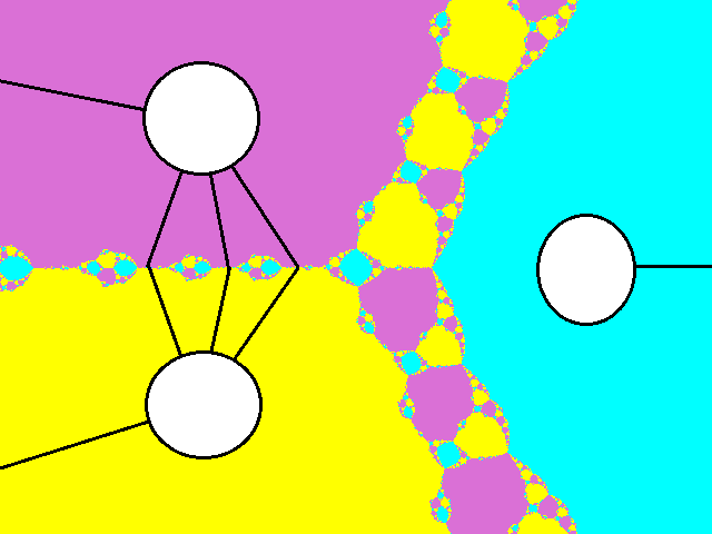
Figure 12. The graphs $Y^{II}_{\lambda}(\zeta,\eta)$ (left) and $Y^{I}_{\lambda}(\kappa)$ (right).

Theorem 8.3.

1. Fix $\lambda\in\Omega_{0}$, then with suitable choices of $\zeta,\eta,\kappa$, at least one of the graphs $Y^{I}_{\lambda}(\kappa),Y^{II}_{\lambda}(\zeta,\eta)$ is an admissible puzzle.

2. If we further assume that $N^{k}_{\lambda}(0)\in\cup_{\varepsilon=1}^{3}\partial B_{\lambda}^{\varepsilon}$ for some $k\geq 0$, then the Lebesgue measure of the Julia set $J(N_{\lambda})$ is zero, and with respect to the admissible puzzle, we have ${\rm Imp}(x)=\{x\}$ for each point $x\in J(N_{\lambda})$. Moreover, the intersection of any shrinking closed puzzle pieces is a singleton.

The first statement is proven in [Ro08, Proposition 5.4], the second statement follows from Theorems 8.1, 8.2.

9. Rigidity and boundary regularity of $\partial\mathcal{H}^{\varepsilon}_{0}$

The aim of this section is to show that all the boundaries $\partial\mathcal{H}_{0}^{\varepsilon}$ are Jordan curves. By the symmetry of the parameter space $\mathcal{X}$, it suffices to prove the results in the fundamental domain $\mathcal{X}_{FD}$. By Remark 3.3, our task is further reduced to show that $\partial\mathcal{H}_{0}^{1}\cap\overline{\Omega}$ is a Jordan arc.

The main ingredient of the proof is the following rigidity theorem:

Theorem 9.1.

Given two parameters $\mathbf{\lambda}_{1},\lambda_{2}\in\Omega$. Assume that the internal rays $R^{1}_{\lambda_{1}}(t),R^{1}_{\lambda_{2}}(t)$ both land at the free critical point $0$ in the corresponding dynamical planes. Then we have $\lambda_{1}=\lambda_{2}$.

When $t$ is rational, the maps $N_{\lambda_{1}}$ and $N_{\lambda_{2}}$ are post-critically finite. In this case, the proof is same as that of Lemma 4.7 (applying Thurston’s Theorem). We omit the details.

Our main effort is to treat the technical case: $t$ is irrational. In this case, the maps are post-critically infinite and Thurston’s Theorem is not available. Instead, an important role of the Yoccoz puzzle theory will emerge. An essential step in the proof of Theorem 9.1 is a QC-criterion, due to Kozlovski, Shen and van Strien [KSS]. Let $U\subsetneq\mathbb{C}$ be a simply connected planar domain and $z\in U$. The shape of $U$ about $z$ is defined by:

$${S}(U,z)=\sup_{x\in\partial U}|x-z|/\inf_{x\in\partial U}|x-z|.$$

Lemma 9.2 (QC-criterion).

Let $\phi:\Omega\rightarrow\tilde{\Omega}$ be a homeomorphism between two Jordan domains, $k\in(0,1)$ be a constant. Let $X$ be a subset of $\Omega$ such that both $X$ and $\phi(X)$ have zero Lebesgue measures. Assume the following holds:

1. $|\bar{\partial}\phi|\leq k|{\partial}\phi|$ a.e. on $\Omega\backslash X$.

2. There is a constant $M>0$ such that for all $x\in X$, there is a sequence of open topological disks $D_{1}\Supset D_{2}\Supset\cdots$ containing $x$, satisfying that

(a). $\bigcap_{j}\overline{D_{j}}=\{x\}$, and

(b). $\sup_{j}S(D_{j},x)\leq M$,   $\sup_{j}S(\phi(D_{j}),\phi(x))<\infty.$

Then $\phi$ is a $K$-quasi-conformal map, where $K$ depends on $k$ and $M$.

We remark that this QC-criterion is a simplified version of [KSS, Lemma 12.1], with a slightly difference in the second assumption (that is, we replace a sequence of round disks in [KSS] by a sequence of disks with uniformly bounded shape), and the original proof goes through without any problem.

Proof of Theorem 9.1 when $t$ is irrational. The proof consists of three steps, and the Yoccoz puzzle theory plays an important role in the proof.

Step 1 (Same Head’s angle) We first show that $\boldsymbol{h}(\lambda_{1})=\boldsymbol{h}(\lambda_{2})$.

If not, without loss of generality, we assume $0<\boldsymbol{h}(\lambda_{1})<\boldsymbol{h}(\lambda_{2})<1/2$. We claim $(\boldsymbol{h}(\lambda_{1}),\boldsymbol{h}(\lambda_{2}))\cap\Xi\neq\emptyset$. This is because if $(\boldsymbol{h}(\lambda_{1}),\boldsymbol{h}(\lambda_{2}))\cap\Xi=\emptyset$, then by Lemma 5.4, we see that $\boldsymbol{h}(\lambda_{1})$ takes the form $p/2^{q}$ and $\boldsymbol{h}(\lambda_{2})$ takes the form $p/(2^{q}-1)$. By Theorem 5.8 and Corollary 5.10, the parameter ray $\mathcal{R}^{1}_{0}(\boldsymbol{h}(\lambda_{1}))$ lands at $\lambda_{1}$. By Lemma 7.3, the internal ray $R_{\lambda_{1}}^{1}(\boldsymbol{h}(\lambda_{1}))$ would land at $0\in\partial{B_{\lambda_{1}}^{1}}$. This would imply that $t=\boldsymbol{h}(\lambda_{1})$ is rational, which is impossible by assumption.

Therefore, by Lemma 5.4, the open interval $(\boldsymbol{h}(\lambda_{1}),\boldsymbol{h}(\lambda_{2}))$ contains a component of $(0,1/2)\setminus\Xi$, say $(t_{1},t_{2})\Subset(\boldsymbol{h}(\lambda_{1}),\boldsymbol{h}(\lambda_{2}))$. It’s obvious that $\lambda_{1},\lambda_{2}$ are contained in two impressions $\mathcal{I}_{\alpha},\mathcal{I}_{\beta}$ with $\alpha\leq t_{1}<t_{2}\leq\beta$, respectively. By Lemma 7.3, in the $\lambda_{1}$-dynamical plane, the internal ray $R_{\lambda_{1}}^{1}(\alpha)$ lands at $0$; in the $\lambda_{2}$-dynamical plane, the internal ray $R_{\lambda_{2}}^{1}(\beta)$ lands at $0$. This contradicts our assumption.

Step 2 (Topological conjugacy) There is a topological conjugacy $\psi$ between $N_{\lambda_{1}}$ and $N_{\lambda_{2}}$, which is holomorphic in the Fatou set of $N_{\lambda_{1}}$.

The construction of $\psi$ is based on the Yoccoz puzzle theory, as follows:

It’s known from Step 1 that $\boldsymbol{h}(\lambda_{1})=\boldsymbol{h}(\lambda_{2})$ and $\Theta_{\lambda_{1}}=\Theta_{\lambda_{2}}$. By the construction of the articulated rays (see Theorem 6.1), we know that if $L_{\lambda_{1}}(\zeta)$ is an articulated ray for $N_{\lambda_{1}}$, then $L_{\lambda_{2}}(\zeta)$ is an articulated ray for $N_{\lambda_{2}}$, and vice versa. As a consequence, we can define the same type of Yoccoz puzzles $Y^{I}_{\lambda}(\kappa)$ and $Y^{II}_{\lambda}(\zeta,\eta)$ for $\lambda=\lambda_{1},\lambda_{2}$. The assumption that $R^{1}_{\lambda_{1}}(t),R^{1}_{\lambda_{2}}(t)$ both land at $0$ implies that if $Y^{I}_{\lambda_{1}}(\kappa)$ (resp. $Y^{II}_{\lambda_{1}}(\zeta,\eta)$) is admissible for $N_{\lambda_{1}}$, then $Y^{I}_{\lambda_{2}}(\kappa)$ (resp. $Y^{II}_{\lambda_{2}}(\zeta,\eta)$) is admissible for $N_{\lambda_{2}}$, and vice versa.

Now we fix a pair of admissible puzzles, say $(Y^{\nu}_{\lambda_{1}},Y^{\nu}_{\lambda_{2}})$. For the reader’s convenience, we recall some definitions from Section 8. The puzzle piece of depth $d\geq 0$, denoted by $P_{d}^{\lambda}$, is a connected component of $\mathbb{\widehat{C}}\setminus N_{\lambda}^{-d}(Y^{\nu}_{\lambda})$. For any $z\in J(N_{\lambda})$, no matter whether the orbit the critical point $0$ meets the puzzle $Y^{\nu}_{\lambda}$, the set

$$P_{d,\lambda}^{*}(z)=\bigcup_{z\in\overline{P_{d}^{\lambda}}}\overline{P_{d}^{\lambda}}$$

is always a closed topological disk.

We first construct a homeomorphism $\psi_{0}$ from the $\lambda_{1}$-dynamical plane to the $\lambda_{2}$-dynamical plane in the following way:

Set $\widehat{\psi}_{0}|_{B_{\lambda_{1}}^{\varepsilon}}=(\phi_{\lambda_{2}}^{\varepsilon})^{-1}\circ\phi_{\lambda_{1}}^{\varepsilon},\varepsilon=1,2,3$. This $\widehat{\psi}_{0}$ can be extended to $\overline{B_{\lambda_{1}}^{\varepsilon}}$ because the boundaries $\partial B_{\lambda_{1}}^{\varepsilon}$ are Jordan curves. Then we are able to extend $\widehat{\psi}_{0}$ to the complementary set $\mathbb{\widehat{C}}\setminus(\cup_{\varepsilon}\overline{B_{\lambda_{1}}^{\varepsilon}})$, which consists of countably many disk components. This extension can be made by interpolation since we have already known the boundary information. In this way, we get an extension of $\widehat{\psi}_{0}$, say $\psi_{0}$. We make an additional plausible requirement for $\psi_{0}$, that is, $\psi_{0}(Y^{\nu}_{\lambda_{1}})=Y^{\nu}_{\lambda_{2}}$.

Then, we can lift $\psi_{0}$ to $\psi_{1}$ so that $\psi_{0}\circ N_{\lambda_{1}}=N_{\lambda_{2}}\circ\psi_{1}$ and $\psi_{1}|_{\cup_{\varepsilon}B_{\lambda_{1}}^{\varepsilon}}=\psi_{0}|_{\cup_{\varepsilon}B_{\lambda_{1}}^{\varepsilon}}$. The lift process is feasible because in the corresponding dynamical planes, the itineraries of the critical point $0$ are same with respect to the corresponding Yoccoz puzzles. Moreover, we can lift infinitely many times and get a sequence of homeomorphisms $\psi_{k}$, satisfying that $\psi_{k}\circ N_{\lambda_{1}}=N_{\lambda_{2}}\circ\psi_{k+1}$ and $\psi_{k+1}|_{N_{\lambda_{1}}^{-k}(\cup_{\varepsilon}B_{\lambda_{1}}^{\varepsilon})}=\psi_{k}|_{N_{\lambda_{1}}^{-k}(\cup_{\varepsilon}B_{\lambda_{1}}^{\varepsilon})}$ for all $k\geq 0$. Note that the requirement $\psi_{0}(Y^{\nu}_{\lambda_{1}})=Y^{\nu}_{\lambda_{2}}$ implies that $\psi_{k}$ preserves the puzzle pieces up to depth $k$ (namely, $\psi_{k}(N_{\lambda_{1}}^{-k}(Y^{\nu}_{\lambda_{1}}))=N_{\lambda_{2}}^{-k}(Y^{\nu}_{\lambda_{2}})$). By Theorem 8.3, for every point $z\in J(N_{\lambda_{1}})$, the shrinking sequence of closed disks

$$P_{1,\lambda_{1}}^{*}(z)\supset P_{2,\lambda_{1}}^{*}(z)\supset P_{3,\lambda_{1}}^{*}(z)\supset\cdots$$

has impression ${\rm Imp}_{\lambda_{1}}(z)=\bigcap_{k}P_{k,\lambda_{1}}^{*}(z)=\{z\}$. The sequence

$$\psi_{1}(P_{1,\lambda_{1}}^{*}(z)),\psi_{2}(P_{2,\lambda_{1}}^{*}(z)),\psi_{3}(P_{3,\lambda_{1}}^{*}(z)),\cdots$$

is a sequence of shrinking closed disks in the $\lambda_{2}$-dynamical plane. Again by Theorem 8.3, the intersection $\bigcap_{k}\psi_{k}(P_{k,\lambda_{1}}^{*}(z))$ consists of a single point, which is denoted by $\rho(z)$.

We define a map $\psi:\mathbb{\widehat{C}}\rightarrow\mathbb{\widehat{C}}$ by

$$\psi(z)=\begin{cases}\lim_{k\rightarrow\infty}\psi_{k}(z),\ &\text{ if }z\in\mathbb{\widehat{C}}\setminus J(N_{\lambda_{1}}),\\ \rho(z),\ &\text{ if }z\in J(N_{\lambda_{1}}).\end{cases}$$

It’s easy to see that $\psi$ is holomorphic in the Fatou set of $N_{\lambda_{1}}$. The continuity and injectivity of $\psi$ follows from Theorem 8.3. It’s also clear that $\psi$ preserves the puzzle pieces of all depths and $\psi$ is surjective. So $\psi$ is a homeomorphism. Since $\psi$ is conjugacy between $N_{\lambda_{1}}$ and $N_{\lambda_{2}}$ in the Fatou set, it is actually a global conjugacy, by continuity.

Step 3 (Rigidity) The conjugacy $\psi$ is a quasi-conformal map.

By Theorem 8.3, we know that the Julia sets $J(N_{\lambda_{1}})$ and $J(N_{\lambda_{2}})$ both have zero Lebesgue measures. To show that $\psi$ is quasi-conformal, by Lemma 9.2, it suffices to show that there is a constant $M>0$ such that for any point $z\in J(N_{\lambda_{1}})$, there is a sequence of open topological disks $D_{1}\Supset D_{2}\Supset\cdots$ containing $x$, satisfying that

(a). $\bigcap_{j}\overline{D_{j}}=\{x\}$, and

(b). $\sup_{j}S(D_{j},x)\leq M$,   $\sup_{j}S(\psi(D_{j}),\psi(x))<\infty.$

The proof is very similar to [QRWY, Section 5.4], with a slight difference. For completeness and the reader’s convenience, we include the details here.

We decompose the Julia set $J(N_{\lambda})$ (here $\lambda$ can be either $\lambda_{1}$ or $\lambda_{2}$) into three disjoint sets:

$$J_{\lambda}^{0} = J(N_{\lambda})\cap\big{(}\cup_{k\geq 0}N_{\lambda}^{-k}(Y_{\lambda}^{\nu})\big{)},$$

$$J_{\lambda}^{1} = \{z\in J(N_{\lambda})\setminus J_{\lambda}^{0};\ 0\notin\omega(z)\},$$

$$J_{\lambda}^{2} = \{z\in J(N_{\lambda})\setminus J_{\lambda}^{0};\ 0\in\omega(z)\},$$

where $\omega(z)$ is the $\omega$-limit set of $z$, defined as $\{y\in J(N_{\lambda});\text{ there exist }n_{k}\rightarrow\infty\text{ such that }N_{\lambda}^{n_{k}}(z)\rightarrow y\}$.

Case 1: Points in $J_{\lambda}^{0}$. By the construction of the Yoccoz puzzle $Y_{\lambda}^{\nu}$, the set $J_{\lambda}^{0}$ is countable, forward invariant (that is $N_{\lambda}(J_{\lambda}^{0})\subset J_{\lambda}^{0}$), and each point in $J_{\lambda}^{0}$ is preperiodic. Note also $J_{\lambda}^{0}$ contains only finitely many periodic points, all are repelling.

Let $z\in J_{\lambda}^{0}$ be a repelling periodic point with period say $p$, then there are two small topological disks $U,V$ in a linearizable neighborhood of $z$, both containing $z$ so that $N_{\lambda}^{p}(U)=V$ and $U\Subset V$. By pulling back $V$ via $N_{\lambda}^{kp}$, we get a sequence of neighborhoods of $z$, say

$$V_{0}(z)\Supset V_{1}(z)\Supset V_{2}(z)\Supset\cdots$$

with $V_{0}(z)=V$, such that $N_{\lambda}^{kp}:V_{k}(z)\rightarrow V_{0}(z)$ is a conformal map for all $k\geq 1$. By the shape distortion [QWY, Lemma 6.1],

$$S(V_{k}(z),z)\leq C(m_{z})\cdot S(V_{1}(z),z),\ \forall k\geq 2,$$

where $C(m_{z})$ is a constant depending only on $m_{z}={\rm mod}(V_{0}(z)\setminus\overline{V_{1}}(z))$.

For any aperiodic point $z\in J_{\lambda}^{0}$, there is a smallest number $\ell\geq 1$ so that $N_{\lambda}^{\ell}(z)$ is periodic. Then by pulling back the sequence of neighborhoods of $V_{k}(N_{\lambda}^{\ell}(z))$ of $N_{\lambda}^{\ell}(z)$, we get a sequence of neighborhoods $V_{k}(z)$ of $z$. Again by the shape distortion, we get

$$S(V_{k}(z),z)\leq C(m_{N_{\lambda}^{\ell}(z)})\cdot S(V_{1}(N_{\lambda}^{\ell}(z)),N_{\lambda}^{\ell}(z)).$$

For any periodic point $z\in J_{\lambda_{1}}^{0}$, set $m_{z}^{*}={\rm mod}\psi((V_{0}(z)\setminus\overline{V_{1}}(z))$. Take

$$M_{0}=\max\{C(m_{z})\cdot S(V_{1}(z),z);z\in J_{\lambda_{1}}^{0}\text{is periodic}\},$$

$${M}_{0}^{*}=\max\{C(m_{z}^{*})\cdot S(\psi(V_{1}(z)),\psi(z));z\in J_{\lambda_{1}}^{0}\text{ is periodic}\},$$

then for all $z\in J_{\lambda_{1}}^{0}$,

$$\sup_{j}S(V_{j}(z),z)\leq M_{0},\ \sup_{j}S(\psi(V_{j}(z)),\psi(z))\leq{M}^{*}_{0}<\infty.$$

Case 2: Points in $J_{\lambda}^{1}$. In this case, there is a integer $d_{0}\geq 0$ such that $N_{\lambda}^{k}(z)\notin P_{d_{0}}^{\lambda}(0)$ for all $k\geq 1$. Then we can find a sequence of integers $k_{j}$ and a point $w\in J(N_{\lambda})\setminus J_{\lambda}^{0}$ so that $N_{\lambda}^{k_{j}}(z)\rightarrow w$ as $j\rightarrow\infty$. By passing to a subsequence, we assume that $N_{\lambda}^{k_{j}}(z)\in P_{d_{0}}^{\lambda}(w)$ for all $j$. It’s clear that the degree of $N_{\lambda}^{k_{j}}:P_{d_{0}+k_{j}}^{\lambda}(z)\rightarrow P_{d_{0}}^{\lambda}(w)$ is at most two. Take a small number $r>0$ so that ${\rm mod}(P_{d_{0}}^{\lambda}(w)\setminus\overline{D_{w}^{r}})\geq 1$, where $D_{w}^{r}$ is the open Euclidean disk centered at $w$ with radius $r$. When $j$ is large, we have $N_{\lambda}^{k_{j}}(z)\in D_{w}^{r/2}$, let $V_{j}(z)$ be the component of $N_{\lambda}^{-k_{j}}(D_{w}^{r})$ containing $z$. Then by the shape distortion [QWY, Lemma 6.1], for large $j$,

$$S(V_{j}(z),z)\leq C\cdot S(D_{w}^{r},N_{\lambda}^{k_{j}}(z))\leq C\cdot\frac{r+r/2}{r-r/2}=3C,$$

here $C$ is a universal constant.

Note that the above shape control holds when $\lambda=\lambda_{1}$, and the upper bound is a universal constant. When $\lambda=\lambda_{2}$, the upper bound of the shape distortion depends on $z$, this can be seen from the following estimate:

$$S(\psi(V_{j}(z)),\psi(z)) \leq C_{1}\cdot S(\psi(D_{w}^{r}),\psi(N_{\lambda_{1}}^{k_{j}}(z)))$$

$$\leq C_{1}\sup_{\zeta\in\psi(D_{w}^{r/2})}S(\psi(D_{w}^{r}),\zeta)<\infty,$$

where $C_{1}$ depends on the modulus of $\psi(D_{w}^{r}\setminus\overline{D_{w}^{r/2}})$, which turns out to be related to $z\in J_{\lambda_{1}}^{1}$.

Case 3: Points in $J_{\lambda}^{2}$. We first look at the free critical point $0$. If $0\notin\omega(0)$, then we may choose a sequence of topological disks $V_{j}(0)$ with uniformly bounded shape as Case 2. For any $z\in J_{\lambda}^{2}$, just as the proof of Case 2, by pulling back the sequence of $V_{j}(0)$, we get a sequence of disks $V_{j}(z)$ surrounding $z$ with uniformly bounded shapes.

The case $0\in\omega(0)$ is more delicate and it is our main focus. In this case, for each $d\geq 0$, let $\tau_{Y}(d)\in[0,d]$ be first integer $k$ such that $0\in N_{\lambda}^{d-k}(P_{d}^{\lambda}(0))$. The function $\tau_{Y}$ is called the Yoccoz $\tau$-function. It satisfies $\tau_{Y}(d+1)\leq\tau_{Y}(d)+1$. It’s clear that the assumption $0\in\omega(0)$ implies that $\limsup_{d}\tau_{Y}(d)=\infty$. There are two possibilities for $\liminf_{d}\tau_{Y}(d)$, either $\liminf_{d}\tau_{Y}(d)\leq L<\infty$ or $\liminf_{d}\tau_{Y}(d)=\infty$. We treat these two cases separately.

Case 3.1 $\liminf_{d}\tau_{Y}(d)\leq L<\infty$. Choose $n_{2}>n_{1}>n_{0}\geq L$ such that $P_{n_{2}}^{\lambda}(0)\Subset P_{n_{1}}^{\lambda}(0)\Subset P_{n_{0}}^{\lambda}(0)$. We see that $\tau_{Y}^{-1}(n_{0})$ is an infinite set, and we write $\tau_{Y}^{-1}(n_{0})=\{k_{1},k_{2},\cdots\}$. By the definition of $\tau_{Y}$, the map $N_{\lambda}^{k_{j}}:P_{n_{0}+k_{j}}^{\lambda}(0)\rightarrow P_{n_{0}}^{\lambda}(0)$ has degree two, for all $j$. For each $j$, let $l_{j}\geq 0$ be the smallest integer such that $N_{\lambda}^{l_{j}}(N_{\lambda}^{k_{j}}(0))\in P_{n_{2}}^{\lambda}(0)$. Then for all $j$, the degree of $N_{\lambda}^{k_{j}+l_{j}}:P_{n_{0}+k_{j}+l_{j}}^{\lambda}(0)\rightarrow P_{n_{0}}^{\lambda}(0)$ is at most $2\cdot 2^{n_{2}-n_{0}}$. For any $z\in J_{\lambda}^{2}$, and any $j\geq 0$, let $m_{j}\geq 0$ be the first integer such that $N_{\lambda}^{m_{j}}(z)\in P_{n_{2}+k_{j}+l_{j}}^{\lambda}(0)$, with the same discussion as above, we see that

$${\rm deg}(N_{\lambda}^{m_{j}}:P_{n_{0}+k_{j}+l_{j}+m_{j}}^{\lambda}(z)\rightarrow P_{n_{0}+k_{j}+l_{j}}^{\lambda}(0))\leq 2\cdot 2^{n_{2}-n_{0}}.$$

This implies that, for all $j$,

$${\rm deg}(N_{\lambda}^{m_{j}+k_{j}+l_{j}}:P_{n_{0}+k_{j}+l_{j}+m_{j}}^{\lambda}(z)\rightarrow P_{n_{0}}^{\lambda}(0))\leq 4\cdot 4^{n_{2}-n_{0}}.$$

By the shape distortion [QWY, Lemma 6.1],

$$S(P_{n_{1}+k_{j}+l_{j}+m_{j}}^{\lambda}(z),z)\leq C_{2}\cdot S(P_{n_{1}}^{\lambda}(0),0)<+\infty,$$

here $C_{2}$ depends on ${\rm mod}(P_{n_{0}}^{\lambda}(0)\setminus\overline{P_{n_{1}}^{\lambda}(0)})$, independent of $z\in J_{\lambda}^{2}$ and $j$.

Case 3.2 $\liminf_{d}\tau_{Y}(d)=\infty$. By a very technical construction of enhanced nests, we have the following property:

There exist a constant $m>0$ and a sequence of critical puzzle pieces

$$P_{d_{1}}^{\lambda}(0)\Supset P_{l_{1}}^{\lambda}(0)\Supset P_{k_{1}}^{\lambda}(0)\Supset P_{d_{2}}^{\lambda}(0)\Supset P_{l_{2}}^{\lambda}(0)\Supset P_{k_{2}}^{\lambda}(0)\cdots$$

satisfying that

(a) $\bigcap\overline{P_{d_{j}}^{\lambda}(0)}=\{0\}$;

(b) ${\rm mod}(P_{d_{j}}^{\lambda}(0)\setminus\overline{P_{l_{j}}^{\lambda}(0)})\geq m,\ \ {\rm mod}(P_{l_{j}}^{\lambda}(0)\setminus\overline{P_{k_{j}}^{\lambda}(0)})\geq m,\ \forall j\geq 1$ ;

(c) Both $P_{d_{j}}^{\lambda}(0)\setminus\overline{P_{l_{j}}^{\lambda}(0)}$ and $P_{l_{j}}^{\lambda}(0)\setminus\overline{P_{k_{j}}^{\lambda}(0)}$ avoid the free critical orbit, for all $j$.

See [KSS, Section 8] for the enhanced nest construction in a more general setting, see [KS] and [QY] for the proof of the complex bounds.

Then by [YZ, Proposition 1], there is a constant $M>0$ such that $S(P_{l_{j}}^{\lambda}(0),0)\leq M$ for all $j$. For any $z\in J_{\lambda}^{2}$ and any $j\geq 1$, let $m_{j}\geq 0$ be the first integer such that $N_{\lambda}^{m_{j}}(z)\in P_{k_{j}}^{\lambda}(0)$. It follows that ${\rm deg}(N_{\lambda}^{m_{j}}:P_{m_{j}+k_{j}}^{\lambda}(z)\rightarrow P_{k_{j}}^{\lambda}(0))\leq 2$. By the above property (c), we have

$${\rm deg}(N_{\lambda}^{m_{j}}:P_{m_{j}+d_{j}}^{\lambda}(z)\rightarrow P_{d_{j}}^{\lambda}(0))\leq 2.$$

By the shape distortion, we have

$$S(P_{m_{j}+l_{j}}^{\lambda}(z),z)\leq C_{3}\cdot S(P_{l_{j}}^{\lambda}(0),0)\leq C_{3}M,$$

here the constant $C_{3}$ depends on $m$ but independent of $z$ and $j$.

This completes the proof of Step 3. Since $\psi$ is conformal on the Fatou set and the Julia set has zero Lebesgue measure (see Theorem 8.3), this $\psi$ is a Möbius map. Note that $\lambda_{1},\lambda_{2}$ are in the fundamental domain, we have $\lambda_{1}=\lambda_{2}$, completing the proof of the theorem. $\Box$

Theorem 9.3.

The boundary $\partial\mathcal{H}_{0}^{1}$ is a Jordan curve.

Proof.

We first show that $\partial\mathcal{H}_{0}^{1}$ is locally connected. For $t\in[0,1/2]$, recall that $\mathcal{I}_{t}$ is the impression of the parameter ray $\mathcal{R}_{0}^{1}(t)$. If $\mathcal{I}_{t}\cap\Omega\neq\emptyset$, then we take two parameters $\lambda_{1},\lambda_{2}\in\mathcal{I}_{t}\cap\Omega$ (if any) so that $N_{\lambda_{1}}$ and $N_{\lambda_{2}}$ have no parabolic cycles. By Lemma 7.3, the internal rays $R_{\lambda_{1}}^{1}(t),R_{\lambda_{2}}^{1}(t)$ both land at the free critical point $0$, in the corresponding dynamical planes. By Theorem 9.1, we see that $\lambda_{1}=\lambda_{2}$. Therefore

$$\mathcal{I}_{t} = (\mathcal{I}_{t}\cap{\partial\Omega})\cup(\mathcal{I}_{t}\cap\Omega)$$

$$\subset \{0,\sqrt{3}i/2\}\cup\{\text{parabolic parameters}\}\cup\{\text{singleton}\},$$

which means the continuum $\mathcal{I}_{t}$ is contained in a countable set. So $\mathcal{I}_{t}$ is a singleton. Since $t\in[0,1/2]$ is arbitrary, this means that $\partial\mathcal{H}_{0}^{1}\cap\overline{\Omega}$ (hence $\partial\mathcal{H}_{0}^{1}$) is locally connected.

In the following, we will show that if two parameter rays $\mathcal{R}_{0}^{1}(t_{1}),\mathcal{R}_{0}^{1}(t_{2})$ with $t_{1},t_{2}\in[0,1/2]$ land at the same point $\lambda$, then $t_{1}=t_{2}$. This would imply that $\partial\mathcal{H}_{0}^{1}$ is a Jordan curve.

We first show that if one of $t_{1},t_{2}$ is $0$ (resp. $1/2$), then the other would be $0$ (resp. $1/2$). To see this, we only consider the case $t_{1}=0$, the same discussion works for the other case. Note that $0$ is an accumulation point of the set $\partial(\Xi)$ (see Fact 5.5 for its definition). If $t_{2}\in(0,1/2]$, we can find an angle $t_{*}\in\partial(\Xi)$ lying in between $0$ and $t_{2}$. By Theorem 5.8, the parameter rays $\mathcal{R}_{0}^{1}(0),\mathcal{R}_{0}^{1}(t_{2})$ are contained in different components of $\mathbb{C}\setminus([-1/2,1/2]\cup\overline{\mathcal{R}_{0}^{1}}(t_{*})\cup\overline{\mathcal{R}_{0}^{2}}(1-t_{*}))$, contradicting that $\mathcal{R}_{0}^{1}(0)$ and $\mathcal{R}_{0}^{1}(t_{2})$ land at the same point. So we must have $t_{2}=t_{1}=0$.

Now, it suffices to assume that $t_{1},t_{2}\in(0,1/2)$. This assumption implies that $\lambda\in\Omega$. By Lemma 7.3, we know that in the dynamical plane, the internal rays $R_{\lambda}^{1}(t_{1})$ and $R_{\lambda}^{1}(t_{2})$ would land at the same point. It follows from Theorem 4.1 that $t_{1}=t_{2}$, completing the proof. ∎

10. Boundaries of Capture domains

Let $\mathcal{H}\subset\Omega$ be a capture domain of level $k\geq 2$. That is, it is a component of $\mathcal{H}_{k}^{\varepsilon}$ for some $\varepsilon\in\{1,2,3\}$. By Theorem 3.4, the map $\Phi_{\mathcal{H}}:\mathcal{H}\rightarrow{\mathbb{D}}$ defined by $\Phi_{\mathcal{H}}(\lambda)=\phi_{\lambda}^{\varepsilon}(N_{\lambda}^{k}(0))$ parameterizes $\mathcal{H}$. The parameter ray $\mathcal{R}_{\mathcal{H}}(t)$ in $\mathcal{H}$, with angle $t\in\mathbb{S}=\mathbb{R}/\mathbb{Z}$, is defined by

$$\mathcal{R}_{\mathcal{H}}(t)=\Phi_{\mathcal{H}}^{-1}(\{re^{2\pi it};0<r<1\}).$$

For any $t\in\mathbb{S}$ and any integer $j\geq 1$, we define an open sector as follows:

$$\mathcal{S}_{\mathcal{H},j}(t)=\Phi_{\mathcal{H}}^{-1}(\{re^{2\pi i\theta};r\in(1-1/j,1),\theta\in(t-1/j,t+1/j)\}).$$

The impression $\mathcal{I}_{\mathcal{H}}(t)$ of the parameter ray $\mathcal{R}_{\mathcal{H}}(t)$ is defined by

$$\mathcal{I}_{\mathcal{H}}(t)=\bigcap_{j\geq 1}\overline{\mathcal{S}_{\mathcal{H},j}(t)}.$$

It’s a standard fact that $\mathcal{I}_{\mathcal{H}}(t)$ is a connected and compact set. Our goal in this section is to show that $\mathcal{I}_{\mathcal{H}}(t)$ is a singleton, which implies that $\partial{\mathcal{H}}$ is locally connected.

Before further discussion, we give an observation for $\mathcal{H}$. By Corollary 5.10, all the maps in $\mathcal{H}$ have the same Head’s angle $\alpha$ of the form ${p\over 2^{n}-1}$, where $(\beta,\alpha)$ is some connected component of $(0,1/2)\setminus\Xi$. Therefore $\mathcal{H}$ is contained in $V(\beta,\alpha)\cap\Omega_{0}$, see Lemma 5.11. In particular, we have $\mathcal{\overline{H}}\subset\Omega$.

When $\lambda\in\mathcal{H}$, we define the set $U_{\lambda}$ to be the Fatou component of $N_{\lambda}$ containing the free critical point $0$. Clearly, the center $c_{\lambda}$ of $U_{\lambda}$, defined as the unique point $c_{\lambda}\in U_{\lambda}$ satisfying $N_{\lambda}^{k}(c_{\lambda})=b_{\varepsilon}(\lambda)$, moves continuously with respect to $\lambda\in\mathcal{{H}}$. It’s also obvious that the center map $\lambda\mapsto c_{\lambda}$ has a continuous extension to $\partial\mathcal{H}$. Therefore, when $\lambda\in\partial\mathcal{H}$, the point $c_{\lambda}$ is well-defined and we define $U_{\lambda}$ to be the unique Fatou component of $N_{\lambda}$ containing $c_{\lambda}$. In this way, the set $U_{\lambda}$ is designated for all $\lambda\in\mathcal{\overline{H}}$.

Lemma 10.1.

For any $t\in[0,1)$ and any $\lambda\in\mathcal{I}_{\mathcal{H}}(t)\setminus(\partial\mathcal{H}_{0}^{1}\cup\partial\mathcal{H}_{0}^{2})$, we have $0\in\partial U_{\lambda}$ and the internal ray $R_{U_{\lambda}}(t)=(N_{\lambda}^{k}|_{U_{\lambda}})^{-1}(R_{\lambda}^{\varepsilon}(t))$ lands at $0$.

Proof.

Note that for any $\lambda\in\mathcal{I}_{\mathcal{H}}(t)\setminus(\overline{\mathcal{H}_{0}^{1}\cup\mathcal{H}_{0}^{2}})\subset\Omega$, there is a disk neighborhood $\mathcal{U}$ of $\lambda$ contained in $\Omega\setminus(\overline{\mathcal{H}_{0}^{1}\cup\mathcal{H}_{0}^{2}})$.

We first claim that for any $\varepsilon\in\{1,2,3\}$, the boundary $\partial B_{u}^{\varepsilon}$ moves holomorphically with respect to $u\in\mathcal{U}$. To see this, fix some $u_{0}\in\mathcal{U}$, we define a map $h:\mathcal{U}\times B_{u_{0}}^{\varepsilon}\rightarrow\mathbb{\widehat{C}}$ by $h(u,z)=(\phi_{u}^{\varepsilon})^{-1}\circ\phi_{u_{0}}^{\varepsilon}(z)$. It satisfies:

(1). Fix any $z\in B_{u_{0}}^{\varepsilon}$, the map $u\mapsto h(u,z)$ is holomorphic;

(2). Fix any $u\in\mathcal{U}$, the map $z\mapsto h(u,z)$ is injective;

(3). $h(u_{0},z)=z$ for all $z\in B_{u_{0}}^{\varepsilon}$.

These properties imply that $h$ is a holomorphic motion parameterized by $\mathcal{U}$, with base point $u_{0}$. By the Holomorphic Motion Theorem (see [GJW] or [Slo]), there is a holomorphic motion $H:\mathcal{U}\times\mathbb{\widehat{C}}$ extending $h$ and for any $u\in\mathcal{U}$, we have $H(u,\partial B_{u_{0}}^{\varepsilon})=\partial B_{u}^{\varepsilon}$. Therefore $\partial B_{u}^{\varepsilon}$ moves holomorphically with respect to $u\in\mathcal{U}$. The claim is proved.

It follows that for any $p\geq 0$, the set $N_{u}^{-p}(\partial B_{u}^{\varepsilon})$ moves continuously in Hausdorff topology with respect to $u\in\mathcal{U}$. By the assumption $\lambda\in\mathcal{I}_{\mathcal{H}}(t)\setminus(\partial\mathcal{H}_{0}^{1}\cup\partial\mathcal{H}_{0}^{2})$, there exist a sequence of parameters $\{u_{n}\}$ in $\mathcal{H}$ and a sequence of angles $\{t_{n}\}$, such that

$$u_{n}\rightarrow\lambda,\ t_{n}\rightarrow t\text{ as }n\rightarrow\infty,\text{ and }N_{u_{n}}^{k}(0)\in R_{u_{n}}^{\varepsilon}(t_{n})\subset B_{u_{n}}^{\varepsilon}\text{ for all }n.$$

By the continuity of $u\mapsto\partial B_{u}^{\varepsilon}$ (which also implies the continuity of the internal rays with respect to the parameter), we have $N_{\lambda}^{k}(0)\in\partial B_{\lambda}^{\varepsilon}$ and the internal ray $R_{\lambda}^{\varepsilon}(t)$ lands at $N_{\lambda}^{k}(0)$. By the continuity of $u\mapsto N_{u}^{-k}(\partial B_{u}^{\varepsilon})$ for $u\in\mathcal{U}$ and the fact $N_{\lambda}^{k}(R_{U_{\lambda}}(t))=R_{\lambda}^{\varepsilon}(t)$, we have that $0\in\partial U_{\lambda}$ and $R_{U_{\lambda}}(t)$ lands at $0$. ∎

To show that $\partial{\mathcal{H}}$ is a Jordan curve, we need two lemmas, whose proofs are very technical.

Lemma 10.2.

For each $t$, let $\mathcal{I}_{\mathcal{H}}^{*}(t)=\mathcal{I}_{\mathcal{H}}(t)\setminus(\partial\mathcal{H}_{0}^{1}\cup\partial\mathcal{H}_{0}^{2})$. Then $\mathcal{I}_{\mathcal{H}}^{*}(t)$ is either empty or a singleton.

Proof.

It’s clear that $\mathcal{I}_{\mathcal{H}}^{*}(t)\subset\overline{\mathcal{H}}\subset\Omega_{0}=\Omega\setminus(\mathcal{H}_{0}^{1}\cup\mathcal{H}_{0}^{2})$. Recall that $\mathcal{H}$ is a component of $\mathcal{H}_{k}^{\varepsilon}$ for some $\varepsilon\in\{1,2,3\}$.

We shall prove the lemma by contradiction. If it is not true, then there exist a connected and compact subset $\mathcal{E}$ of $\mathcal{I}_{\mathcal{H}}^{*}(t)$ containing at least two points. By Lemma 10.1, the internal ray $R_{U_{\lambda}}(t)$ lands at $0$ for all $\lambda\in\mathcal{E}$. It is worth observing that for all $\lambda\in\mathcal{E}$, we have $N_{\lambda}^{k-1}(0)\notin\partial B_{\lambda}^{\varepsilon}$ and $N_{\lambda}^{k}(0)\in\partial B_{\lambda}^{\varepsilon}$. (To see this, if $N_{\lambda}^{k-1}(0)\in\partial B_{\lambda}^{\varepsilon}$, then $N_{\lambda}^{k-1}(0)$ would be a common boundary point of $N_{\lambda}^{k-1}(U_{\lambda})$ and $N_{\lambda}^{k}(U_{\lambda})=B_{\lambda}^{\varepsilon}$. It turns out that $N_{\lambda}^{k-1}(0)$ is a critical point of $N_{\lambda}$. Necessarily, we have $N_{\lambda}^{k-1}(0)=0$. Contradiction.) So by continuity, there is disk neighborhood $\mathcal{D}\subset\Omega_{0}$ of $\mathcal{E}$ such that for all $\lambda\in\mathcal{D}$, we have $N_{\lambda}^{k-1}(0)\notin\overline{B_{\lambda}^{\varepsilon}}$.

Now take two different parameters $\lambda_{1},\lambda_{2}\in\mathcal{E}$. Suppose that $\{1,2,3\}$ can be rewritten as $\{\varepsilon,\varepsilon_{1},\varepsilon_{2}\}$. For $l=1,2$, we define a subset $Z_{\lambda_{1}}^{l}$ of $B^{\varepsilon_{l}}_{\lambda_{1}}$ to be $\{z\in B^{\varepsilon_{l}}_{\lambda_{1}};|\phi^{\varepsilon_{l}}_{\lambda_{1}}(z)|<1/2\}.$ Let

$$J=\{N_{\lambda_{1}}^{j}(0);0\leq j\leq k-1\}\cup{B_{\lambda_{1}}^{\varepsilon}}\cup Z_{\lambda_{1}}^{1}\cup Z_{\lambda_{1}}^{2}.$$

It’s clear that its closure $\overline{J}$ contains the post-critical set of $N_{\lambda_{1}}$. We define a continuous map $h:\mathcal{D}\times J\rightarrow\mathbb{\widehat{C}}$ satisfying:

1. $h(\lambda,z)=(\phi_{\lambda}^{\varepsilon})^{-1}\circ\phi_{\lambda_{1}}^{\varepsilon}(z)$ for all $(\lambda,z)\in\mathcal{D}\times{B_{\lambda_{1}}^{\varepsilon}}$;

2. $h(\lambda,z)=(\phi_{\lambda}^{\varepsilon_{l}})^{-1}\circ\phi_{\lambda_{1}}^{\varepsilon_{l}}(z)$ for all $(\lambda,z)\in\mathcal{D}\times Z_{\lambda_{1}}^{l},\ l=1,2$;

3. $h(\lambda,N_{\lambda_{1}}^{j}(0))=N_{\lambda}^{j}(0)$ for all $\lambda\in\mathcal{D}$ and $0\leq j\leq k-1$.

By definition, $z\mapsto h(\lambda_{1},z)$ is the identity map. The map $h$ is a holomorphic motion parameterized by $\mathcal{D}$, with base point $\lambda_{1}$. By the Holomorphic Motion Theorem (see [GJW, Slo]), there is a holomorphic motion $H:\mathcal{D}\times\mathbb{\widehat{C}}\rightarrow\mathbb{\widehat{C}}$ extending $h$. We consider the restriction $H_{0}=H|_{\mathcal{E}\times\mathbb{\widehat{C}}}$ of $H$. Note that fix any $\lambda\in\mathcal{E}$, the map $z\mapsto H(\lambda,z)$ sends the post-critical set of $N_{\lambda_{1}}$ to that of $N_{\lambda}$, preserving the dynamics on this set. By the lifting property, there is a unique continuous map $H_{1}:\mathcal{E}\times\mathbb{\widehat{C}}\rightarrow\mathbb{\widehat{C}}$ such that $N_{\lambda}(H_{1}(\lambda,z))=H_{0}(\lambda,N_{\lambda_{1}}(z))$ for all $(\lambda,z)\in\mathcal{E}\times\widehat{\mathbb{C}}$ and $H_{1}(\lambda_{1},\cdot)\equiv id$.

Set $\psi_{0}=H_{0}(\lambda_{2},\cdot)$ and $\psi_{1}=H_{1}(\lambda_{2},\cdot)$. Both $\psi_{0}$ and $\psi_{1}$ are quasi-conformal maps, satisfying $N_{\lambda_{2}}\circ\psi_{1}=\psi_{0}\circ N_{\lambda_{1}}$. One may verify that $\psi_{0}$ and $\psi_{1}$ are isotopic rel $\overline{J}$. Again by the lifting property, there is a sequence of quasi-conformal maps $\psi_{j}$ satisfying that

(a). $N_{\lambda_{2}}\circ\psi_{j+1}=\psi_{j}\circ N_{\lambda_{1}}$ for all $j\geq 0$,

(b). $\psi_{j+1}$ and $\psi_{j}$ are isotopic rel $N_{\lambda_{1}}^{-j}(\overline{J})$.

The maps $\psi_{j}$ form a normal family since their dilatations are uniformly bounded above. Let $\psi_{\infty}$ be the limit map of $\psi_{j}$. It is quasi-conformal in $\mathbb{\widehat{C}}$, holomorphic in the Fatou set $F(N_{\lambda_{1}})=\bigcup_{j\geq 0}N_{\lambda_{1}}^{-j}(B_{\lambda_{1}}^{\varepsilon}\cup Z_{\lambda_{1}}^{1}\cup Z_{\lambda_{1}}^{2})$ and satisfies $N_{\lambda_{2}}\circ\psi_{\infty}=\psi_{\infty}\circ N_{\lambda_{1}}$ in $F(N_{\lambda_{1}})$. By continuity, we have $N_{\lambda_{2}}\circ\psi_{\infty}=\psi_{\infty}\circ N_{\lambda_{1}}$ in $\mathbb{\widehat{C}}$. By Theorem 8.3, the Lebesgue measure of the Julia set $J(N_{\lambda_{1}})$ is zero. Therefore $\psi_{\infty}$ is a Möbius map. Since both $\lambda_{1}$ and $\lambda_{2}$ are contained in the fundamental domain $\mathcal{X}_{FD}$, we have $\lambda_{1}=\lambda_{2}$. This contradicts the assumption that $\lambda_{1}\neq\lambda_{2}$. ∎

It follows from Lemma 10.2 that the impression $\mathcal{I}_{\mathcal{H}}(t)$ is either a singleton or contained in $\partial\mathcal{H}_{0}^{1}\cup\partial\mathcal{H}_{0}^{2}$. To analyze the latter case, we shall prove

Lemma 10.3.

If $\mathcal{I}_{\mathcal{H}}(t)\subset\partial\mathcal{H}_{0}^{1}\cup\partial\mathcal{H}_{0}^{2}$, then $\mathcal{I}_{\mathcal{H}}(t)$ is a singleton.

Proof.

Let $\lambda\in\mathcal{I}_{\mathcal{H}}(t)$ be a parameter so that $N_{\lambda}$ has no parabolic cycle. By assumption, either $\lambda\in\partial\mathcal{H}_{0}^{1}$ or $\lambda\in\partial\mathcal{H}_{0}^{2}$.

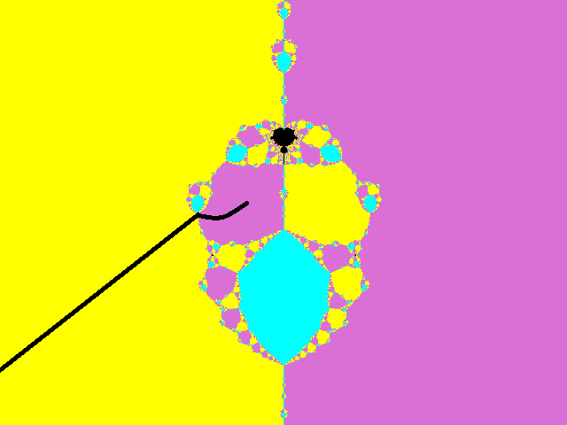
Figure 13. A case that $\mathcal{I}_{\mathcal{H}}(t)\cap\partial\mathcal{H}_{0}^{1}\neq\emptyset$.

If $\lambda\in\partial\mathcal{H}_{0}^{1}$, by Theorem 7.1, the free critical point $0$ of $N_{\lambda}$ is on $\partial B_{\lambda}^{1}$. Let $R_{\lambda}^{1}(\alpha)$ be the internal ray landing at $0$, we will show that

$$2^{k}\alpha=t\ {\rm mod}\ \mathbb{Z},$$

where we recall that $k$ is the level of $\mathcal{H}$.

We prove the assertion by contradiction, mimicking the proof of Lemma 7.3. If the above equation is not true, then by Fact 6.3, there is a graph $G_{\lambda}$ avoiding the free critical orbit of $N_{\lambda}$, an integer $q\geq 0$ and a neighborhood $\mathcal{V}^{\prime}$ of $\lambda$, satisfying that

(a). $G_{u}$ is well-defined and moves continuously when $u\in\mathcal{V}^{\prime}$;

(b). $N_{u}^{-q-k}(G_{u})$ avoids the free critical point $0$ for all $u\in\mathcal{V}^{\prime}$;

(c). when $u=\lambda$, the graph $N_{\lambda}^{-q}(G_{\lambda})$ separates $R_{\lambda}^{1}(2^{k}\alpha)$ and $R_{\lambda}^{1}(t)$.

The third property (c) implies that $N_{\lambda}^{-q}(G_{\lambda})$ also separates $R_{\lambda}^{1}(2^{k}\alpha)$ and a sector neighborhood of $R_{\lambda}^{1}(t)$. The sector neighborhood can be chosen in the following way: we can first choose rational angles $t_{1},t_{2}$ such that

1. $t_{1}<t<t_{2}$ are in counter clockwise order.

2. The internal rays with angles $t_{1},t,t_{2}$ are in the same component of $\mathbb{\widehat{C}}\setminus N_{\lambda}^{-q}(G_{\lambda})$.

3. The closure of the internal rays $R_{u}^{1}(\theta)$ with $\theta\in\{t_{1},t_{2}\}$ are well-defined, avoiding $0,N_{u}(0),\cdots,N_{u}^{q+k}(0)$ and moves continuously in a neighborhood $\mathcal{V}_{0}\subset\mathcal{V}^{\prime}$ of $\lambda$ (by suitable choices of the angles and Fact 4.3).

Let $S_{B_{u}^{1}}(t_{1},t_{2})$ be the open sector which contains $(\phi_{u}^{1})^{-1}\{(0,1/2)e^{2\pi it}\}$ and bounded by $\partial B_{u}^{1}$, $\overline{R_{u}^{1}}(\theta),\theta\in\{t_{1},t_{2}\}$. By the continuity of $N_{u}^{-q-k}(G_{u})$, we see that for all $u\in\mathcal{V}_{0}$, the free critical point $0$ and $(\phi_{u}^{1})^{-1}\{(0,1/2)e^{2\pi i\alpha}\}$ are contained in the same component, say $D_{u}$, of $\mathbb{\widehat{C}}\setminus N_{u}^{-q-k}(G_{u})$, and $D_{u}\cap N_{u}^{-k}(S_{B_{u}^{1}}(t_{1},t_{2}))=\emptyset$. However, the assumption $\lambda\in\mathcal{I}_{\mathcal{H}}(t)$ implies that when $u\in\mathcal{H}\cap\mathcal{V}_{0}\cap\mathcal{S}_{\mathcal{H},j}(t)$ with $1/j<\min\{|t_{1}-t|,|t_{2}-t|\}$, the free critical point $0\in N_{u}^{-k}(S_{B_{u}^{1}}(t_{1},t_{2}))$. Contradiction. This proves that $2^{k}\alpha=t\ {\rm mod}\ \mathbb{Z}$.

If $\lambda\in\partial\mathcal{H}_{0}^{2}$, again by Theorem 7.1, the free critical point $0$ of $N_{\lambda}$ is on $\partial B_{\lambda}^{2}$. Let $R_{\lambda}^{2}(\beta)$ be the internal ray landing at $0$, using the same argument as above, we can show that

$$2^{k}\beta=t\ {\rm mod}\ \mathbb{Z}.$$

Therefore each $\lambda\in\mathcal{I}_{\mathcal{H}}(t)$ either corresponds to a map $N_{\lambda}$ having a parabolic cycle or is contained in the following finite set

$$\{\text{the landing point of the parameter ray }\mathcal{R}_{0}^{\varepsilon}(\alpha);2^{k}\alpha=t,\ \varepsilon=1,2\}.$$

So $\mathcal{I}_{\mathcal{H}}(t)$ is at most a countable set. The connectivity of $\mathcal{I}_{\mathcal{H}}(t)$ implies that it is a singleton. ∎

Now we are ready to prove the main result of this section:

Theorem 10.4.

$\partial\mathcal{H}$ is a Jordan curve.

Proof.

We know from the previous two lemmas that $\partial\mathcal{H}$ is locally connected. Assume by contradiction that there are two parameter rays $\mathcal{R}_{\mathcal{H}}(t_{1}),\mathcal{R}_{\mathcal{H}}(t_{2})$ with $t_{1}\neq t_{2}$, landing at the same point $\lambda\in\partial\mathcal{H}$. Let’s look at the dynamical plane of $N_{\lambda}$, it follows from Theorem 4.1 that the internal rays $R_{U_{\lambda}}(t_{1})$ and $R_{U_{\lambda}}(t_{2})$ would land at two different points. Using the same idea of proof as Lemma 10.3, by Fact 6.3, there is a graph $G_{\lambda}$ avoiding the free critical orbit of $N_{\lambda}$, an integer $q\geq 0$ and a neighborhood $\mathcal{V}^{\prime}$ of $\lambda$ satisfying that

(a). $G_{u}$ is well-defined and continuous for $u\in\mathcal{V}^{\prime}$;

(b). $N_{u}^{-q}(G_{u})$ avoids the free critical point $0$;

(c). when $u=\lambda$, $N_{\lambda}^{-q}(G_{\lambda})$ separates $R_{U_{\lambda}}(t_{1})$ and $R_{U_{\lambda}}(t_{2})$.

The continuity of $N_{u}^{-q}(G_{u})$ implies that it would separated two sector neighborhoods of the internal arcs with angles $t_{1}$ and $t_{2}$ in $U_{u}$ for $u\in\mathcal{V}^{\prime}$ (here, the internal arc with angle $\theta\in\{t_{1},t_{2}\}$ refers to the section of the set $R_{U_{u}}(\theta)$ that is closed to the center $c_{u}$). This implies that $\lambda$ can not be the landing points of the parameter rays $\mathcal{R}_{\mathcal{H}}(t_{1})$ and $\mathcal{R}_{\mathcal{H}}(t_{2})$ simultaneously. It contradicts our assumption. ∎

11. Proof of Theorems 1.3 and 1.4

In this section, we will prove Theorems 1.3 and 1.4. To prove these results, it suffices to work in the fundamental domain $\mathcal{X}_{FD}$.

Up to now, we have shown that $\partial\mathcal{H}_{0}^{1}$ and $\partial\mathcal{H}_{0}^{2}$ are Jordan curves. This implies that each parameter ray $\mathcal{R}_{0}^{1}(t)$ with $t\in[0,1/2]$ (resp. $\mathcal{R}_{0}^{2}(\theta)$ with $\theta\in[1/2,1]$) converges to a point on $\partial{\mathcal{H}_{0}^{1}}$ (resp. $\partial{\mathcal{H}_{0}^{2}}$).

Let $\nu_{1}(t),\nu_{2}(\theta)$ be the landing points of the parameter rays $\mathcal{R}_{0}^{1}(t),\mathcal{R}_{0}^{2}(\theta)$ respectively. By Caratheodory’s Theorem, the maps

$$\nu_{1}:[0,1/2]\rightarrow\partial\mathcal{H}_{0}^{1}\cap\overline{\Omega},\ \ \nu_{2}:[1/2,1]\rightarrow\partial\mathcal{H}_{0}^{2}\cap\overline{\Omega}$$

both are homeomorphisms. By Theorem 5.8, we have

$$\nu_{1}(t)=\nu_{2}(1-t),\ \forall\ t\in\partial(\Xi).$$

It’s known from Lemma 5.4 that $\Xi\cup\{0\}$ is the accumulation set of $\partial(\Xi)$. Therefore by the continuity of $\nu_{\varepsilon}$, we get

$$\nu_{1}(t)=\nu_{2}(1-t),\ \forall\ t\in\Xi\cup\{0\}.$$

Let’s look at the Head’s angles for the maps in $\mathcal{X}_{FD}\setminus(\mathcal{H}_{0}^{1}\cup\mathcal{H}_{0}^{2})=\Omega_{0}\cup\{\sqrt{3}i/2\}$. By Corollary 5.10, we see that

$$\boldsymbol{h}(\nu_{1}(t))=t,\ \forall\ t\in\partial(\Xi).$$

By Corollary 5.13, we see that $\boldsymbol{h}$ is continuous at the points $\nu_{1}(t)$ with $t\in\Xi\setminus\partial(\Xi)$. Therefore by continuity and Fact 5.2 we have

$$\boldsymbol{h}(\nu_{1}(t))=t,\forall\ t\in\Xi.$$

This equality implies that the map $\boldsymbol{h}:\Omega_{0}\cup\{\sqrt{3}i/2\}\rightarrow\Xi$ is surjective.

To finish, we show that this map is also monotone. In fact, by Corollary 5.10 and Fact 5.2, we know that

(a) If $\theta\in\Xi\cap\Theta_{dya}$, then $\boldsymbol{h}^{-1}(\theta)$ is a singleton.

(b) If $\theta\in\Xi\cap\Theta_{per}$, then $\boldsymbol{h}^{-1}(\theta)$ is a closed disk $D$ minus a boundary point $w$. Assume that $\theta$ takes the form $\frac{p}{2^{q}-1}$, then this closed disk $D$ is bounded exactly by the curve

$$\nu_{1}\Big{(}\Big{[}\frac{p}{2^{q}},\frac{p}{2^{q}-1}\Big{]}\Big{)}\bigcup\nu_{2}\Big{(}\Big{[}1-\frac{p}{2^{q}},1-\frac{p}{2^{q}-1}\Big{]}\Big{)}$$

and the boundary point $w$ is exactly $\nu_{1}(\frac{p}{2^{q}})$.

(c) If $\theta\in\Xi\setminus\partial(\Xi)$, we see from the above discussion that $\boldsymbol{h}^{-1}(\theta)$ is also a singleton.

The discussions in this section can be summarized as follows:

The fiber $\boldsymbol{h}^{-1}(\theta)$ over $\theta\in\Xi$ is a singleton if and only if $\theta$ is not $\tau$-periodic. If $\theta$ is $\tau$-periodic, then $\boldsymbol{h}^{-1}(\theta)$ is homeomorphic to a closed disk minus a boundary point.

This completes the proof of Theorem 1.4, hence also Theorem 1.3.

References

- [Ah] L. V. Ahlfors. Lectures on quasi-conformal mappings , volume 38 of University Lecture Series, Amer. Math. Soc., 2006.
- [Ba] K. Barański. From Newton’s method to exotic basins Part I: The parameter space. Fund. Math. 158 (1998).
- [Be] W. Bergweiler, Newton’s method and a class of meromorphic functions without wandering domains, Ergodic Theory Dynam. Systems 13 (1993) 231-247.
- [B] P. Blanchard. The Dynamics of Newton’s Method, Proceedings of the Symposia in Applied Mathematics, Volume 49, 1994
- [BH] B. Branner and J. H. Hubbard. The iteration of cubic polynomials, Acta Math. 169(1992), 229-325.
- [BR] X. Buff and J. Rückert. Virtual Immediate Basins of Newton Maps and Asymptotic Values. IMRN, 2006 Article ID 65498, Pages 1-18
- [C] A. Cayley. Desiderata and suggestions: no. 3. the Newton-Fourier imaginary problem. Amer. J. Math. 2 (1879), no. 1, 97.
- [CGS] J. H. Curry, L. Garnett, and D. Sullivan, On the iteration of a rational function: computer experiments with Newton’s method. Comm. Math. Phys. Volume 91, Number 2 (1983), 267-277.
- [CG] L. Carleson and T. Gamelin, Complex Dynamics, Springer-Verlag, New York, 1993.
- [DH1] A. Douady and J. H. Hubbard, On the dynamics of polynomial-like mappings, Ann. Sci. École Norm. Sup. 18(1985), 287-343.
- [DH2] A. Douady, J. H. Hubbard, A proof of Thurston’s topological characterization of rational functions. Acta Math. 171, 263-297 (1993)
- [GJW] F. Gardiner, Y. Jiang and Z. Wang, Holomorphic motions and related topics. Geometry of Riemann Surfaces, London Mathematical Society Lecture Note Series, No. 368, 2010, 166-193.
- [Ha] M. Haruta, Newton¡¯s method on the complex exponential function, Trans. Amer. Math. Soc. 351 (1999) 2499-2513.
- [He] J. Head, The combinatorics of Newton’s method for cubic polynomials, Thesis, Cornell University (1987).
- [HP] J. H. Hubbard, P Papadopol. Newton’s method applied to two quadratic equations in viewed as a global dynamical system.
- [H] J. H. Hubbard, Local connectivity of Julia sets and bifurcation loci: three theorems of J.-C. Yoccoz, in Topological Methods in Modern Mathematics, 467-511 (L. R. Goldberg and A. V. Phillips, eds.), Publish or Perish, Houston, TX, 1993.
- [HSS] J. Hubbard, D. Schleicher and S. Sutherland, How to find all roots of complex polynomials by Newton’s method. Invent. Math. 146 (2001), 1-33.
- [KL] J. Kahn and M. Lyubich. The Quasi-additivity Law in Conformal Geometry. Ann. Math. 169 (2009) 561-593
- [KSS] O. Kozlovski, W. Shen, S. van Strien, Rigidity for real polynomials. Ann. Math. 165(2007), 749-841.
- [KS] O. Kozlovski, S. van Strien. Local connectivity and quasi-conformal rigidity of non-renormalizable polynomials. Proc. London Math. Soc. (2) 99 (2009), 275–296.
- [LMS1] R. Lodge, Y. Mikulich, D. Schleicher. Combinatorial properties of Newton maps. arXiv:1510.02761
- [LMS2] R. Lodge, Y. Mikulich, D. Schleicher. A classification of postcritically finite Newton maps. arXiv:1510.02771.
- [Luo] J. Luo, Newton’s method for polynomials with one in ection value, preprint, Cornell University 1993.
- [L] M. Lyubich. On the Lebesgue measure of the Julia set of quadratic polynomial. arXiv:math/9201285v1.
- [Ma] A. Manning. How to be sure of finding a root of a complex polynomial using Newton’s method, Bol. Soc. Brasil. Mat. 22 (1992) 157-177.
- [May] S. Mayer, Newton’s method for transcendental functions, Diplomarbeit, TU München, 2002.
- [MS] S. Mayer and D. Schleicher. Immediate and virtual basins of Newton’s method for entire functions. Ann. Inst. Fourier (Grenoble),
- [Mãné] R. Mañé. Hyperbolicity, sinks and measure in one dimensional dynamics. Comm. Math. Phys. 100, 495-524 (1985). Erratum: Comm. Math. Phys. 112, 721-724 (1987).
- [MSS] R. Mañé, P. Sad, and D. Sullivan. On the dynamics of rational maps. Ann. Sci. Éc. Norm. Sup. 16(1983), 193-217.
- [Mc1] C. McMullen. Families of rational maps and iterative root-finding algorithms, Ann. of Math. 125 (1987), 467-493.
- [Mc2] C. McMullen, Complex Dynamics and Renormalization, Ann. of Math. Studies 135, Princeton Univ. Press, Princeton, NJ, 1994.
- [Mi] Y. Mikulich, Newton’s Method as a Dynamical System. Thesis, Jacobs University Bremen, 2011.
- [MRS] Y. Mikulich, J. Rückert, D. Schleicher. A Combinatorial classification of post-critically fixed Newton maps, arXiv:1010.5280v2.
- [M1] J. Milnor, Dynamics in One Complex Variable (3rd Edition). Ann. of Math. Studies 160, Princeton Univ. Press, Princeton, NJ, 2006.
- [M2] J. Milnor, Local Connectivity of Julia Sets: Expository Lectures in The Mandelbrot Set, Theme and Variations (Tan Lei, ed.), London, Math. Soc. Lecture Note Series 274, 67-116, Cambridge Univ. Press, Cambridge, 2000.
- [P] F. Przytycki, Remarks on the simple connectedness of basins of sinks for iterations of rational maps, Collection: Dynamical systems and ergodic theory, Warsaw, 1986. Banach Center Publications 23 (1989), 229-235.
- [QWY] W. Qiu, X. Wang, Y. Yin. Dynamics of McMullen maps. Adv. Math. 229(2012), 2525-2577.
- [QRWY] W. Qiu, P. Roesch, X. Wang, Y. Yin. Hyperbolic components of McMullen maps. Ann. Sci. École Norm. Sup. 48 (2015) 703-737.
- [QY] W. Qiu and Y. Yin, Proof of the Branner-Hubbard conjecture on Cantor Julia sets. Science in China (Series A) 52(2009), 45-65.
- [Ro] R. Roeder. Topology for the basins of attraction of Newton’s Method in two complex variables: linking with currents. J. Geom. Anal. 17 (1) 107-146, 2007.
- [R97] P. Roesch. Topologie locale des méthodes de Newton cubiques. PhD Thesis, Ecole Normale Supérieure de Lyon. 1997.
- [Ro99] P. Roesch, Puzzles de Yoccoz pour les applications à allure rationnelle. L’Enseign. Math. 45 (1999), 133-168.
- [Ro99] P. Roesch, Topologie locale des méthodes de Newton cubiques: plan paramétrique. Comptes Rendus de l’Academie des Sciences. Volume 328, Issue 2, 1999, 151-154.
- [Ro07] P. Roesch. Hyperbolic components of polynomials with a fixed critical point of maximal order. Ann. Sci. École Norm. Sup. 40 (2007), 1-53.
- [Ro08] P. Roesch. On local connectivity for the Julia set of rational maps: Newton¡¯s famous example. Annals of Mathematics. 168 (2008), 1-48.
- [Rü1] J. Rückert. Newton’s Method as a Dynamical System. PhD Thesis. International University Bremen. 2006
- [Rü2] J. Rückert. Rational and Transcendental Newton Maps, In: M. Lyubich, M. Yampolsky (eds.) Holomorphic Dynamics and Renormalization.
- [RS] J. Rückert and D. Schleicher, On Newton’s method for entire functions. J. London Math. Soc. 75 3 (2007), 659-676.
- [S] D. Schleicher. On the Efficient Global Dynamics of Newton’s Method for Complex Polynomials. arXiv:1108.5773.
- [Sh] M. Shishikura, The connectivity of the Julia set and fixed points, in Complex dynamics: families and friends (Ed. by D. Schleicher), A. K. Peters (2009).
- [Slo] Z. Slodkowski. Holomorphic motions and polinomial hulls. Proc. Amer. Math. Soc. 111, 347-355,1991.
- [Tan] L. Tan, Branched coverings and cubic Newton maps. Fund. Math. 154(3) (1997), 207-260.
- [W] X. Wang. A decomposition theorem for Herman maps. Adv. Math. 267(2014) 307-359.
- [YZ] Y. Yin, Y. Zhai. No invariant line fields on cantor Julia sets. Forum Math. 22 (2010) 75-94.