Revised calibration for near- and mid-infrared images from $\sim 4000$ pointed observations with AKARI/IRC

Abstract

The Japanese infrared astronomical satellite AKARI performed $\sim 4000$ pointed observations for 16 months until the end of 2007 August, when the telescope and instruments were cooled by liquid Helium. Observation targets include solar system objects, Galactic objects, local galaxies, and galaxies at cosmological distances. We describe recent updates on calibration processes of near- and mid-infrared images taken by the Infrared Camera (IRC), which has nine photometric filters covering 2–27 $\mu$m continuously. Using the latest data reduction toolkit, we created calibrated and stacked images from each pointed observation. About 90% of the stacked images have a position accuracy better than $1.5^{\prime\prime}$. Uncertainties in aperture photometry estimated from a typical standard sky deviation of stacked images are a factor of $\sim$ 2–4 smaller than those of AllWISE at similar wavelengths. The processed images together with documents such as process logs as well as the latest toolkit are available online.

1 Introduction

AKARI is the Japanese infrared (IR) satellite (Murakami et al., 2007) launched on 2006 February 21 and operated until 2011 November 24. The AKARI mission consists of several different phases of observations: a commissioning period prior to scientific operation called “Performance Verification (PV)” phase, followed by Phase 1 and 2 for scientific observations, the second PV phase, and Phase 3 for only near-IR (NIR) observations. Phase 1 started on 2006 May 8 and lasted for half a year. Most of time during Phase 1 was devoted to the all-sky survey at mid- and far-IR wavelengths. Phase 2 started on 2006 November 10, and many pointed observations together with supplemental all-sky survey were performed during this phase until 2007 August 26, as the cryogenic liquid Helium boiled off. After the second PV phase to optimize the system performance under warmer environments, Phase 3 started on 2008 June 1 (Onaka et al., 2010). Pointed observations only at NIR wavelengths were carried out until 2010 February 15. No science observations were performed between then and the end of the AKARI operation.

The Infrared Camera (IRC) is designed for observations at NIR and mid-IR (MIR) wavelengths (Onaka et al., 2007) while the Far-Infrared Surveyor (FIS) is for those at far-IR wavelengths (Kawada et al., 2007). The IRC has three channels (NIR, MIR-S, and -L) and each channel has three photometric filters together with spectroscopic dispersers. These nine filters are named as N2, N3, N4, S7, S9W, S11, L15, L18W, and L24. The first letter indicates the channel, the numbers indicate its representative wavelength in $\mu$m, and “W” denotes wide band. They cover 2–27 $\mu$m continuously and are useful to detect various objects at various redshifts and/or at various conditions. For example, emission and absorption features due to interstellar dust at NIR and MIR wavelengths can be used to trace interstellar medium at different conditions (e.g. Sakon et al. (2007); Mori et al. (2012)) and star-forming galaxies at different redshifts (e.g. Pearson et al. (2010); Takagi et al. (2010)). The filter response curve, i.e. the wavelength coverage, of each filter is presented in Onaka et al. (2007). As illustrated in Figure 1, the field of view (FoV) of NIR and MIR-S almost coincides, while that of MIR-L is $\sim 20^{\prime}$ away, each FoV being $\gtrsim 10^{\prime}$ on one side.

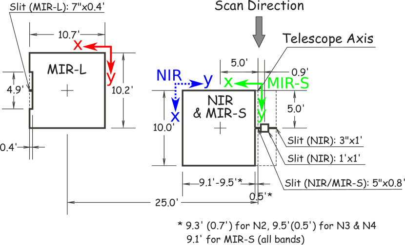
Figure 1: The field of views of the three channels of AKARI/IRC, revised from Onaka et al. (2007). The x- and y-axis directions of images from each channel are indicated by arrows: blue dotted for NIR, green solid for MIR-S, and red solid for MIR-L. The scan direction is along the ecliptic meridian.

AKARI pointed observations were carried out based on proposals classified as Large Survey, Mission Program, Open Time, and Director’s Time. Their targets span a wide range of objects such as asteroids in the solar system (e.g. Hasegawa et al. (2008); Müller et al. (2014)), evolved stars in our Galaxy (e.g. Ita et al. (2007); Arimatsu et al. (2011a)), interstellar dust in local and nearby galaxies (e.g. Kaneda et al. (2008); Yamagishi et al. (2010); Egusa et al. (2013)), and distant galaxies (e.g. Takagi et al. (2010); Murata et al. (2013)). Among them, the Large Magellanic Cloud (LMC) and the North Ecliptic Pole (NEP) regions were extensively observed as the Large Survey projects (Ita et al., 2008; Kato et al., 2012; Shimonishi et al., 2013; Matsuhara et al., 2006; Lee et al., 2009).

Each pointed observation is identified with one ObsID, which is a combination of targetID (7-digit number) and subID (3-digit number), e.g. 1234567_123. In most cases, subIDs are in the chronological order. There are a few exceptions due to observing conditions. One pointed observation ($\sim 10$ min excluding maneuvers) consists of nine or ten exposure cycles (as the term “exposure frames” used in Onaka et al. (2007)) with filter changes and dithering between the cycles. The astronomical observation template (AOT) defines their combinations for different types of observations as summarized in Table 1. One exposure cycle consists of short and long exposures and the number and duration of these exposures depend on the channels and AOTs. Short exposure frames are useful for observing extremely bright sources and for identifying saturated pixels in long exposure frames. For more detail about the IRC and AOTs, see Onaka et al. (2007). Long exposure durations in Table 1 are from Tanabé et al. (2008).

Summary of IRC AOTs for Phase 1&2 Name filters per channel long exposure frames per filter long exposure durations [sec] dithering NIR MIR-S and -L NIR MIR-S and -L IRC00 1 10 30 44.4 16.4 no IRC02 2 4 12 44.4 16.4 yes IRC03 3 3 9 44.4 16.4 yes IRC04 1$+$spectrometer 1 3 44.4 16.4 no IRC05 1 5 30 65.5 16.4 no

Along with the scientific outcome mentioned above, data processing techniques for IRC images have been improved. Artifacts and point spread function (PSF) shapes for MIR were examined and characterized by Arimatsu et al. (2011b). Tsumura & Wada (2011) investigated and modeled a short-time variation of NIR dark current. Egusa et al. (2013) created a template for MIR dark current and for the earthshine light by combining images from neighbor observations. Temporal variations of MIR-S flat pattern were explored by Murata et al. (2013).

In principle, a user needs to reduce the raw data using the toolkit provided by the AKARI team, but the data reduction often requires experience and knowledge in IR observations. In order to promote using AKARI/IRC data by a wide range of researchers, we have recently included all of the abovementioned improvements into the toolkit and processed all the raw data sets from Phase 1&2 pointed observations except those of failed observations. In addition to the raw data sets, processed and calibrated images along with documents and the latest toolkit have been released on 2015 March 31. All of these products are available from the AKARI observers website. With the advantage of the continuous wavelength coverage, these newly released AKARI/IRC data sets will enable us to explore new science cases as well as the studies originally planned in the proposals.

In this paper, we describe major revisions in the toolkit in §2, present properties of processed and released data in §3, and discuss remaining issues in §4.

2 Data reduction

The IRC imaging toolkit is based on the Image Reduction and Analysis Facility (IRAF) command language with additional tools written in C and Perl. Since the first release on 2007 January 4 (ver. 20070104, named after the release date), several major updates have been applied to the toolkit. The standard flow of the current pipeline processing (ver. 20150331) is outlined in Figure 2. Several preparative or minor steps are not presented to simplify the flow. Among these processes, we here describe important steps that require a specific treatment due to the nature of AKARI/IRC images of pointed observations.

Data presented in this paper are mostly products processed with the default setting. For example, we apply a sub-pixel sampling, so that one original pixel is divided into $2\times 2$ pixels. Signal in a pixel becomes $1/4$ of that of the original pixel after this sub-pixel sampling. We stack long-exposure frames only and use short-exposure frames just for identifying saturated pixels. We apply flux conversion factors from Tanabé et al. (2008) to the stacked images. The unit of final pixel values is $\mu$Jy per pixel. Users can reprocess the raw data with different options, and skip and/or add some steps in order to obtain images best suited for their scientific aims. For more detail of the toolkit tasks and options, see the IRC data users manual available from the AKARI observers website.

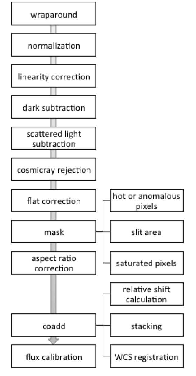
Figure 2: Outline of the standard pipeline processing flow in the IRC imaging toolkit. Several preparative or minor steps are omitted for the sake of visibility.

2.1 Dark frames

During a pointed observation, dark frames were obtained before and after target observations, called pre- and post-dark frames, respectively. For Phase 1&2, we identify three types of temporal variation in IRC dark frames: (i) short-term (i.e. within one pointed observation or $\sim 10$ minutes), (ii) intermediate-term (i.e. over several pointed observations or a few hours), and (iii) long-term (i.e. over the entire observation period or more than a few months). For the short-term variation, we measure the average level of the masked area for spectroscopic observations on each frame during an observation. Since pixels in this area are masked during imaging observations, the average level of these pixels should correspond to the average dark current level. The average level of the same area of the dark frame is also measured and their difference between the object and dark frames (i.e. a constant) is subtracted or added accordingly when the dark frame is subtracted from an object frame. In the following, the latter two variations are described together with hot pixels in MIR frames.

The default setting of the toolkit is to use a model by Tsumura & Wada (2011) for NIR and neighbor dark frames for MIR long exposure frames. We use these default dark frames to calibrate images presented in this paper, i.e. the released data sets.

2.1.1 Model for NIR dark frames

The intermediate-term variation of dark current has been thought to be due to a passage of South Atlantic Anomaly. Tsumura & Wada (2011) investigated this variation for NIR long-exposure frames and found that the variation cannot be fully calibrated by just adding or subtracting the constant. Using more than 4000 pre-dark frames taken in Phase 1&2, they created a model of this dark current variation for each pixel of the NIR array. An accuracy of the model was estimated to be $\sim 1$ ADU, which is about 10% of the typical dark current and corresponds to $\sim 0.3~{}\mu$Jy for NIR long-exposure frames (Tanabé et al., 2008).

2.1.2 Neighbor dark frames for MIR

The long-term variation appears as an increase of hot pixels and is more evident at longer wavelengths. Combining pre-dark frames in each pointed observation (called self-dark) better calibrates this variation than super-dark, which was created by combining $\sim 100$ pre-dark frames taken in the early phase of the satellite operation. However, during a standard pointed observation, only three pre-dark frames were obtained for MIR long exposure, so that the signal-to-noise (S/N) ratio of self-dark is lower than that of super-dark.

In order to obtain a dark frame which represents the long-term variation with a high S/N, Egusa et al. (2013) and Murata et al. (2013) combine pre-dark frames of neighbor pointed observations. Following this strategy, for each ObsID, we combine pre-dark frames from five observations before and after that observation (i.e. 11 observations in total) to create a neighbor dark frame of MIR-S and -L long exposure. The number of frames combined is 33 or more and a typical duration is about one day. By subtracting super or neighbor dark from pre-dark frames, we estimate uncertainties in the dark subtraction process. In Figure 3, histograms of these MIR dark residuals are presented for observations performed on 2006 May 31 (top) and 2007 July 16 (bottom), i.e. around the beginning and the end of Phase 1&2. While the main part of gaussian profiles peaking around zero does not change with time, residuals of the super-dark subtraction (thin black line) have a significant positive tail compared to the neighbor dark subtraction (thick red line) at the later stage of Phase 2 (bottom panels). This result indicates that many hot pixels are not fully corrected after subtracting the super dark. In the top panels, on the other hand, a tail of the black histogram appears on the negative side. It is most likely due to the fact that frames used to create the super dark include those taken after the observation shown in the top panels. Some pixels in the super dark may be affected by hot pixels appearing after this observation. As a result, such pixels are over-subtracted after the super-dark subtraction. Nevertheless, it is clear from this figure that neighbor dark frames are more appropriate than super dark frames for reducing the effect of hot pixels. We estimate the uncertainty of dark subtraction is $\sim 5$ and 4 ADU for MIR-S and -L, respectively, from the width of the main gaussian profiles. These uncertainties are about 10% of the typical dark current and correspond to $\sim 4$ and $10~{}\mu$Jy for MIR-S and -L long-exposure frames, respectively (Tanabé et al., 2008).

Observation date = 2006 May 31

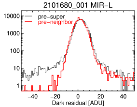
Observation date = 2007 July 16

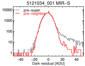
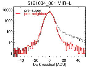
Figure 3: Dark residual [ADU] measured as pre-dark $-$ super-dark (thin black) or pre-dark $-$ neighbor-dark (thick red) frames. Left and right columns are for MIR-S and -L, respectively. Top and bottom rows are for observations performed around the beginning and the end of Phase 1&2, respectively. ObsIDs and channels are presented in the top of each plot.

2.1.3 MIR hot pixels from neighbor dark frames

From these neighbor dark frames, hot pixels are defined as pixels whose values exceed a certain threshold. In the toolkit, the default threshold is $500.0$ ADU and users can adjust it if necessary. In order to determine this default value, we investigated a temporal variation of representative pixels in MIR-L neighbor dark frames, as shown in Figure 4. We found that once a pixel value exceeds $\sim 500$ ADU (i.e. orange and red points in the figure) it stays at the same high level in most cases and its fluctuation becomes larger than the typical dark current, which is $\sim 50$ ADU for MIR. On the other hand, when a pixel value is $\lesssim 100$–$200$ (i.e. green points in the figure), its fluctuation is smaller or comparable to the typical dark current (Note that y-axis of this figure is logarithmic scale). We thus regard such a pixel can be calibrated by the dark subtraction and set the default threshold to be $500.0$ ADU. The number of hot pixels is plotted against observation dates in Figure 5.

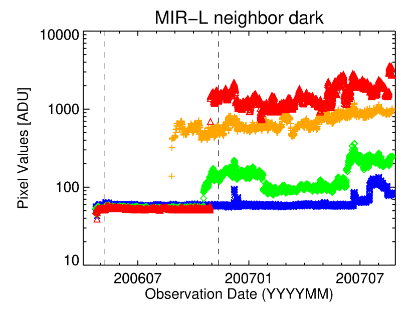
Figure 4: Pixel values [ADU] of four selected pixels in MIR-L neighbor dark frames indicated by different colors. The horizontal axis is observation dates in YYYYMM format. Two vertical dashed lines indicate the start of Phase 1 and 2.

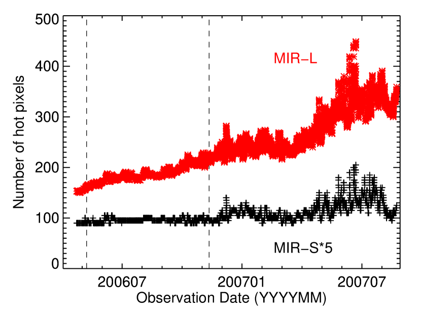
Figure 5: The number of hot pixels identified in neighbor dark frames for MIR-S (black plus, multiplied by 5) and -L (red asterisk). The horizontal axis and the vertical lines are the same as Figure 4.

2.2 Flat pattern

The flat pattern is a distribution of pixel sensitivity on a detector. We create a flat frame for each filter by combining object frames (i.e. sky flat). The default setting of the toolkit is to subtract a constant sky after dividing by a flat frame. In the following part of this subsection, we explain special treatments needed in the flat correction.

2.2.1 Extended ghosts in MIR-L

Arimatsu et al. (2011b) investigated ghost patterns in MIR-S and -L arrays and successfully separated extended ghost (or artificial flat) patterns and “true” flat patterns for L15 and L24. Using these two “true” flat patterns for L15 and L24, Murata et al. (2013) created a “true” flat pattern for L18W. In the toolkit, a difference between observed and “true” flat patterns of each MIR-L filter is treated as an extended ghost pattern and is subtracted from object frames during the flat correction instead of subtracting a constant sky.

2.2.2 The “soramame” pattern in NIR and MIR-S

It has been known that in the bottom right corner of the MIR-S FoV a noticeable pattern was present until 2007 January 7. From its shape, this pattern is called “soramame” (broad bean in Japanese). As a faint but similar pattern was also seen in the bottom left corner of the NIR FoV, its cause is thought to be an obstacle in the light path before the beam splitter. The effect of “soramame” pattern is typically a few percent for NIR and up to 10 percent for MIR-S. In addition, the sky background is less bright in NIR, so that “soramame”-shaped artifact is more prominent in MIR-S.

Murata et al. (2013) investigated a temporal variation of the MIR-S “soramame” shape in detail and found five periods with different shapes. Since the shape was not stable even within one period, Murata et al. (2013) created a “soramame” pattern for each frame from neighbor frames. However, the number of neighbor frames is not always enough to create a neighbor flat for the entire period of Phase 1&2. We thus re-defined the five periods into p1, p23, p4, and p5, and created a flat frame for each MIR-S filter and each period. The period p23 is a combination of the second and third periods defined by Murata et al. (2013). We combined these two periods, since the variation during these periods was small and gradual and thus it was hard to draw a dividing line. It is consistent with the fact that typical patterns for these two periods presented by Murata et al. (2013) (“ii” and “iii” in their Figure 3 (a)) resemble each other. Furthermore, the earthshine light effect (described in §4.4) is significant during the first half of p23. Since we create a flat frame for each period by stacking object frames taken in that period, frames with artificial patterns fixed to the detector coordinates (such as the earthshine light) should not be used. We thus created a flat frame from data only in the latter half of p23 and the toolkit applies it to all the data in p23. The starting date of each period is listed in Table 2.2.2 and the last period, p6, corresponds to the period without “soramame”.

For NIR, the number of frames was smaller and the temporal variation in shape of the artifact was less clear. We thus created one flat frame for each filter for all the periods with “soramame” instead of splitting into four periods.

Flat frames with “soramame” are presented in Figures 6 and 7 for N4 and S7, respectively. The cyan dashed boxes in these two figures enclose the same area on the focal plane (see Figure 1 for the FoV alignment of NIR and MIR-S). A bright circle in the p1 S7 flat is a residual of an observed source. Since the p1 period was short, the number of frames is not enough to remove such residuals and thus the reliability and S/N of the flat for this period are low. We thus decided not to include flat frames for p1 in the toolkit and thus not to deliver the processed data from this period. Note that p1 is in the PV phase.

Starting date of each period for “soramame” artifact Name Date (YYYY-MM-DD) p1 2006-04-22 p23 2006-04-29 p4 2006-12-09 p5 2006-12-15 p6 2007-01-07

Figure 6: A flat frame for N4 to demonstrate “soramame”-shaped artifact within the cyan dashed box, which encloses the same area as those in Figure 7 (Note that the bottom left corner in NIR corresponds to the bottom right corner in MIR-S. See Figure 1 for the FoV alignment and axis directions.).

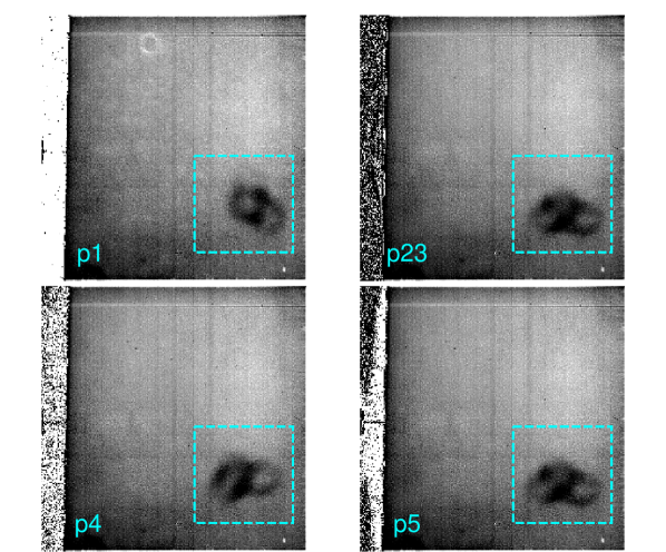
Figure 7: Flat frames for S7 with “soramame” within the cyan dashed boxes in the bottom right corner, which enclose the same area as that in Figure 6 (Note that the bottom left corner in NIR corresponds to the bottom right corner in MIR-S. See Figure 1 for the FoV alignment and axis directions.). From top left to bottom right, the periods are p1, p23, p4, and p5 as indicated in the bottom left corner of each panel. The white circle in the top left of the p1 flat frame is a residual of an observed source due to the small number of frames available during this period. See §2.2.2 for more detail.

2.3 Relative shift between frames

The position of FoV on the sky is not always the same during one pointed observation due to an intentional dithering and/or unintentional jittering and drifting of the satellite’s attitude. For each filter, the shift values in x- and y- direction and the counter-clockwise rotation angle relative to the first frame of a pointed observation are calculated using bright sources within the FoV. The minimum number of the sources used in this calculation is set to seven. In other words, if only six or less sources are found in a frame, no calculation is performed and this frame is excluded from stacking.

For observations without dithering (AOT=IRC00 or IRC05), histograms of these shifts and angle calculated for MIR-S frames are presented in Figure 8 to demonstrate the pointing stability. Histograms for those with dithering (AOT=IRC02 or IRC03) are presented in Appendix B.1. Note that the shift values are calculated after the sub-pixel sampling, so that two pixels in the plot correspond to one original pixel. We fit a gaussian profile to each histogram and find that the histogram for the shift in x-direction has significant wings. This result indicates that the drift was mostly along the x-axis direction of MIR-S images (see Figure 1 for the axis direction), which is consistent with the measured PSF sizes described in §3.4. The drift issue is also discussed in §4.5.

Upper and lower limits to the shift values are set to exclude false matching for MIR-S and -L frames. We manually determine these limits to include most of the wings of the histograms and to be at where the histogram profiles drop steeply. These limits are indicated by blue dashed lines in Figure 8, and given in a constant parameter file of the toolkit. Meanwhile, no such limit is employed for NIR frames. We notice that some of the frames are excluded due to their large drifts rather than the false matching. However, the current toolkit cannot distinguish these two factors, since it only checks shift values of one frame against the corresponding limits. In some cases, the telescope was drifting gradually, so that relative shift values between adjacent frames are small although those with respect to the first frame exceed the limit. These frames can be identified and resurrected by checking difference in shift values between adjacent frames, but such a scheme is not established yet.

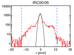
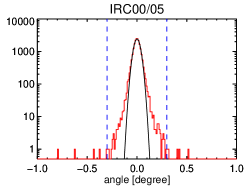
Figure 8: Histogram of relative shift and rotation angle of MIR-S frames for IRC00 and IRC05, i.e. observations without dithering. Pixel numbers are after the sub-pixel sampling, i.e. twice the original value. One pixel is $1.17^{\prime\prime}$ for MIR-S. Black curves represent the results of gaussian fit to the histogram and blue dashed lines indicate the lower and upper limits adopted in the toolkit.

2.4 WCS matching

The World Coordinate System (i.e. Right Ascension and Declination) information from the satellite telemetry was not accurate enough for scientific purposes because of the insufficient absolute accuracy of the attitude and orbit control system and the pointing stability. The toolkit determines the WCS of a stacked image by matching detected sources in the image and sources in the 2MASS (Skrutskie et al., 2006) catalog for NIR or in the Wide-field Infrared Survey Explorer (WISE; Wright et al. (2010)) catalog for MIR-S and -L. We note that the toolkit performs this WCS matching process for each stacked image (i.e. each filter) due to the following reasons: (i) more sources are available in stacked images compared to individual frames (i.e. WCS matching to individual frames is more difficult), and (ii) the FoVs of NIR/MIR-S and MIR-L are $\sim 20^{\prime}$ apart and their absolute roll angle is not confirmed to be stable enough (i.e. WCS information from MIR-S cannot be simply transferred to MIR-L or absolute positions for all the sources found in all the images for one pointed observation cannot be solved all at once). The matching tolerance is set to be $1.5^{\prime\prime}$ at all the wavelengths.

Typical uncertainties in this process are $0.4^{\prime\prime}$, $0.5^{\prime\prime}$, and $0.8^{\prime\prime}$, for NIR, MIR-S, and -L, respectively (See §3.2 and Appendix B.2 for more detail).

3 Results from all-data processing

In this section, we describe how the released data sets were created and their quality such as a position accuracy, image sensitivity, and PSF.

3.1 Process summary

As already mentioned, the sub-pixel sampling is performed and only long exposure frames are stacked. The unit of pixel values is $\mu$Jy per pixel, with the pixel size of $0.723^{\prime\prime}$, $1.17^{\prime\prime}$, and $1.19^{\prime\prime}$, for NIR, MIR-S, and -L, respectively. The Right Ascension and Declination (J2000) of stacked images are available when the WCS matching is successful. The background sky is subtracted before stacking. All the options and parameter settings adopted to create the released data sets are recorded in a log file included in a package for each ObsID (See also Appendix A). A sample of processed images for a pointed observation is presented in Figure 9.

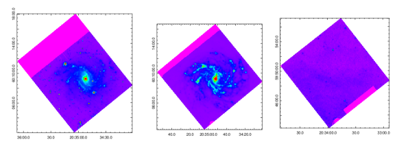
Figure 9: Sample of calibrated and stacked images (N3, S11, and L15 from left to right) from a pointed observation (ObsID=1400620_001) toward a nearby spiral galaxy NGC 6946 in the NIR and MIR-S FoVs. The FoV of MIR-L image is $\sim 20^{\prime}$ away. Coordinates are R.A. and Dec. (J2000). The flux ranges presented are [-10,100], [-100,1000], and [-20,200] $\mu$Jy/pix for N3, S11, and L15, respectively. Magenta area are masked pixels mostly due to the slit for spectroscopic observations.

During the first PV and Phase 1&2, $\sim 4000$ pointed observations were performed with the IRC. When the FIS was the primary instrument to observe a target, the IRC was operated and observing at a field $\sim 20^{\prime}$ away from that of the FIS. These observations are called parallel observations. The FIS was operated either in the slow-scan mode for imaging observations (AOT = FIS01 or FIS02) or in the staring mode for spectroscopic observations (AOT = FIS03). The parallel IRC observations of the latter (i.e. FIS03) are denoted as IRC05, and are included in the released data set. One exposure cycle with photometric filters taken as positional references in the spectroscopic observations (IRC04) is also included. On the other hand, p1 is excluded due to the low S/N of MIR-S flat frames as explained in §2.2.2. We also exclude several observations without any valid data.

The number of observations (i.e. ObsIDs) for the standard observation modes (with each AOT and AOTparameter) is listed in Table 3.1. The AOTparameter, N or L, denotes whether the main target is in the NIR and MIR-S FoVs or in the MIR-L FoV. Figure 10 illustrates the on-sky distribution of imaging (red) and spectroscopic (blue) observations during Phase 1&2. It is clearly seen that many observations are made toward the Galactic plane ($b\sim 0^{\circ}$), NEP ($l\sim 100^{\circ}$, $b\sim 30^{\circ}$), and LMC ($l\sim 280^{\circ}$, $b\sim-30^{\circ}$). The number of observations for each proposal is presented in Appendix A.

The number of observations for the standard observation modes in Phase 1&2      AOT^∗      N^†      L^†      IRC00      12      0      IRC02      1189      370      IRC03      542      151      IRC04      650      230      IRC05      513      252 Observational settings for each AOT are summarized in Table 1.
N and L are the AOT parameter specifying a target in NIR/MIR-S and -L FoVs, respectively. See §3.1 for detail.

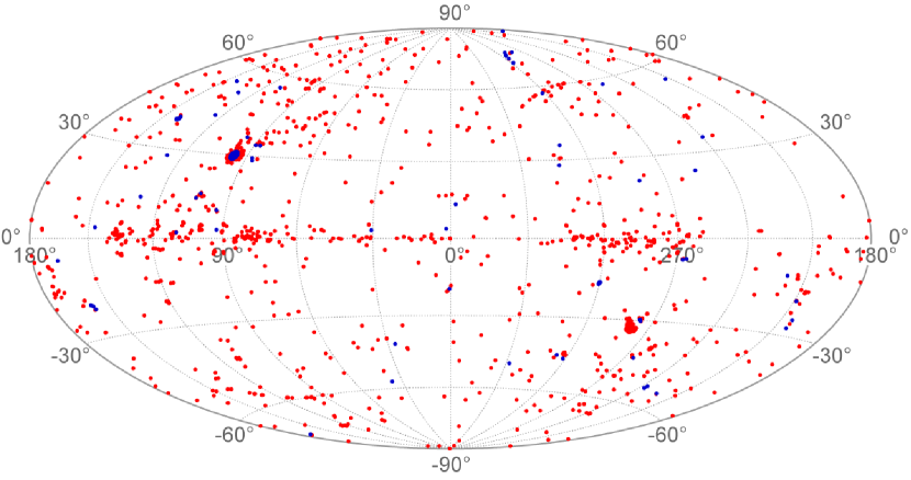
Figure 10: All the pointed observations during Phase 1&2 in the galactic coordinates. Red and blue dots indicate imaging and spectroscopic observations, respectively.

Since the exposure cycle is the same for MIR-S and -L, the relative shift values for MIR-S and -L should also be the same. Meanwhile, the shift calculation for MIR-L is generally more difficult as the number of bright sources at longer wavelengths is smaller. For imaging data, we also created stacked images by using the “coaddLusingS” scheme, in which shift values calculated for MIR-S frames are used to stack MIR-L frames. Among these two stacked images for one MIR-L filter, we selected the better one to be released based on the number of frames used for stacking and the results of WCS matching. In the released data sets, the fraction of stacked images by the “coaddLusingS” scheme is 56%, 70%, and 78% for L15, L18W, and L24, respectively. These fractions are consistent with the general picture mentioned above (i.e. more sources brighter at shorter wavelengths) but not 100%. We deduce that this is due to the different FoVs for MIR-S and -L – when a target is in the MIR-L FoV, the number of bright sources can be larger for MIR-L, resulting in a better result with the original MIR-L shift values.

3.2 Position accuracy

Stacked images with successful WCS matching are defined as “Matched Images”. Typical uncertainties in the WCS matching are $0.4^{\prime\prime}$, $0.5^{\prime\prime}$, and $0.8^{\prime\prime}$ for NIR, MIR-S, and MIR-L, respectively. See Appendix B.2 for more detail. We examined all of the Matched Images visually and rejected an image if most of the sources in that image were displaced $>5^{\prime\prime}$ from catalogued sources. We did not take into account elongated PSFs (see §3.4 and also §4.5) for rejection. Rejected images amount to $\sim 1$% of the Matched Images, and are re-classified as “Failed Images” together with unsuccessful WCS matching. The numbers of Matched and Failed Images for each filter are summarized in Table 3.2. The success rates are calculated as Matched/(Matched+Failed) and $\sim 98$% for NIR and $>90$% for MIR-S. The rate generally decreases with wavelength and is $\sim 50$% for L24. The average success rate for all the stacked images is 87%.

Results of WCS matching N2 N3 N4 S7 S9W S11 L15 L18W L24 All Matched Images 850 2545 1772 2407 1694 2293 2331 1327 1314 16533 Failed Images 14 58 34 258 70 193 339 404 1185 2555 Success Rate 0.98 0.98 0.98 0.90 0.96 0.92 0.87 0.77 0.53 0.87

3.3 Sensitivity

A standard deviation of a background sky signal in stacked images is estimated using data sets from the NEP observations performed during 2006 August and 2007 April, when the earthshine effect (discussed in §4.4) was not significant. A temporal variation for the whole Phase 1&2 is presented in Appendix B.3. For each stacked image, we create a histogram of pixel values and fit a gaussian profile. A typical value of the gaussian profile width, $\sigma$, is adopted as the standard sky deviation. Table 3.3 lists this value for each filter and AOT in units of $\mu$Jy/pixel. Values for IRC02 are not listed as this AOT was not used for the NEP observations, but they should be in between those of IRC03 and IRC05.

Typical standard sky deviation of stacked images from NEP observations [$\mu$Jy/pix] AOT N2 N3 N4 S7 S9W S11 L15 L18W L24 IRC03 0.11 0.079 0.078 0.65 0.70 1.1 2.0 1.9 4.0 IRC05 0.061 0.043 0.042 0.38 0.54 0.75 1.2 1.1 2.6 Measured in stacked images created with sub-pixel sampling.

Note that these values are for the stacked images, i.e. after the sub-pixel sampling, aspect ratio correction, and shift-and-add processes, all of which affect the noise distribution. Especially, the sub-pixel sampling has a significant effect as it divides one pixel into four pixels, resulting in signal in a pixel and thus $\sigma$ of its distribution to be $1/4$ of the original values. We should also note here that this $\sigma$ corresponds to the standard deviation and differs from an uncertainty of the sky level in one image, which should be estimated by the standard error. Taking into account this sub-pixel sampling effect, we estimate the $5\sigma$ sensitivity in aperture photometry. Values for the apertures used in Tanabé et al. (2008) are listed in Table 3.3 in units of mJy.

Typical $5\sigma$ sensitivity in aperture photometry from NEP observations [mJy] AOT N2 N3 N4 S7 S9W S11 L15 L18W L24 IRC03 0.058 0.042 0.041 0.29 0.31 0.49 0.89 0.84 1.8 IRC05 0.032 0.023 0.022 0.17 0.24 0.33 0.53 0.49 1.2

We compare this sensitivity for IRC05 with that of WISE, whose four filters at 3.4, 4.6, 12, and 22 $\mu$m can be compared to N3, N4, S11, and L24, respectively. While WISE sensitivities depend on a position on the sky, the $5\sigma$ values for the COSMOS field (Scoville et al., 2007) in the AllWISE Data Release are 0.054, 0.071, 0.73, and 5.0 mJy, respectively. These values are $\sim 2$–4 larger than those for IRC05.

3.4 PSF

The shape and size of the PSF in a stacked image depends on the instrumental PSF, the pointing stability, and the accuracy of relative shift calculations. While PSFs differ from the gaussian profile especially for MIR-L images (Arimatsu et al., 2011b), we here provide information on PSF sizes by fitting a two-dimensional (2D) gaussian profile.

We measure PSF sizes on stacked images from NEP observations performed during 2006 October and 2006 December. Histograms of measured sizes (major and minor axis lengths in FWHM of the fitted 2D gaussian) are created for each filter and each AOT (see Appendix B.4). Typical PSF sizes are estimated from the peak of these histograms and listed in Table 3.4. From this table, it is clear that NIR PSFs are more elongated than those of MIR. We attribute these NIR elongated PSFs to a larger amount of the jitter and/or drift during longer exposure times compared to MIR. As summarized in Table 1, the exposure time of one NIR long exposure frame for IRC03 and IRC05 is 44.4 sec and 65.5 sec, respectively, while that for one MIR long exposure frame is 16.4 sec for all AOTs (see also Tanabé et al. (2008)). On the other hand, the number of frames used for stacking is typically a factor of two or more smaller for IRC03 than for IRC05. If errors in shift calculations have a significant effect, PSF sizes of IRC05 should be larger than those of IRC03. Although the NIR PSF sizes of IRC05 are slightly larger than those of IRC03, the difference is only comparable to the width of their histograms and no such trend is seen in the PSF sizes for MIR (Table 3.4). We thus conclude that the pointing uncertainty due to the jitter and/or drift during an exposure has a dominant effect on the PSF shape rather than the uncertainty of relative shift calculations. In addition, we find that major axes of PSFs are roughly along the y-axis for NIR images and x-axis for MIR images. These PSF elongation directions both correspond to the cross-scan direction of the satellite (see Figure 1). This result indicates that the drift was more significant in that direction. (See Appendix B.4 for more detail.)

Typical PSF size of stacked images in FWHM [arcsec] from NEP observations AOT N2 N3 N4 S7 S9W S11 L15 L18W L24 IRC03 $3.9\times 5.4$ $3.3\times 6.2$ $3.3\times 6.0$ $6.3\times 5.0$ $6.5\times 5.3$ $6.4\times 5.5$ $6.2\times 5.4$ $6.7\times 6.1$ $7.5\times 6.5$ IRC05 $3.9\times 5.7$ $3.4\times 6.4$ $3.3\times 6.4$ $6.2\times 4.9$ $6.6\times 5.2$ $6.8\times 5.5$ $6.2\times 5.5$ $6.7\times 5.8$ $7.2\times 6.7$

3.5 Confusion

Using the typical PSF sizes measured above and NEP observations performed with IRC05 and during 2006 August and 2007 April, we examine if stacked images are limited by the source confusion. We should note here that the source confusion condition (i.e. the local source density) depends primarily on the Galactic latitude. Since the NEP field is not close to the Galactic plane ($b\sim 30^{\circ}$), the confusion limit can be higher for observations toward lower Galactic latitudes.

For a stacked image, we identify sources brighter than $5\sigma$ and perform aperture photometry. The aperture radius for a source and sky is the same as Tanabé et al. (2008). Following the procedures adopted by Wada et al. (2008), the source number density per beam is calculated, where the beam area is given by $\pi({\rm PSF_{maj}~{}[FWHM]}/2.35)\times({\rm PSF_{min}~{}[FWHM]}/2.35)$ and ${\rm PSF_{maj}}$ and ${\rm PSF_{min}}$ are major and minor axis length of PSF listed in Table 3.4, respectively. If this density exceeds $1/30$, we regard the image is confusion limited and derive the confusion limit flux (c.f. Condon (1974); Hogg (2001)).

Among 161 pointed observations toward the NEP region, $\sim 50$–60 stacked images are available for each filter. We find that none of the images are confusion limited except for one N2 and one N3 images that have severe artificial noises. Meanwhile, Wada et al. (2008) create a large mosaic of the NEP field combining $\sim 200$ AKARI/IRC pointed observations. For NIR, they estimate the $5\sigma$ sensitivity to be $\sim 10~{}\mu$Jy and find that the source number densities are close to the limit (i.e. $1/30$). Since our sensitivities for aperture photometry at NIR are about twice their values, our conclusion above is consistent with their results.

3.6 Flux calibration stability

Following Tanabé et al. (2008), we use photometric standard stars to check the flux calibration factors and their stability during Phase 1&2. The flux calibration factor is defined as the ratio of the flux predicted by models (Cohen et al., 1996, 1999, 2003a, 2003b; Cohen, 2003) to the observed flux, which is measured by aperture photometry on frames after the aspect ratio correction. We find that the calibration factor was stable within $\sim$10%, noting that the error includes uncertainties of the standard star models. No significant dependence on time is found, as already reported by Tanabé et al. (2008).

4 Remaining artifacts and issues

In this section, we describe artifacts and issues still remaining in the processed images. All of them are also explained in more detail in the IRC data users manual.

4.1 NIR detector anomalies

NIR detector anomalies such as column pulldown and muxbleed are not removed. Both of them appear when a bright source falls into the detector FoV. The former is a decrease of the signal of pixels in the same column with the source, resulting in a negative vertical stripe. The latter is a cyclic pattern in the signal of pixels in the same row as the source, resulting in short stripes aligned horizontally. Note that these artifacts cannot be removed by dithering as they move with the source. Murata et al. (2013) masked out columns and rows with an object brighter than a certain limit before stacking, which worked well for their NEP data sets since the field was observed many times with different rotation angles. During one pointed observation, a rotation angle does not vary significantly (Figure 8), so that these anomalies still remain in stacked images.

4.2 Ghost patterns

The ghost is an artifact due to reflections between optical elements. As described in §2.2.1, the extended ghost pattern for the background sky in MIR-L is removed during the flat calibration. Other ghost patterns due to bright compact objects still remain in the processed images. Arimatsu et al. (2011b) identified small-scale ghosts that appear close ($\sim 1^{\prime}$) to a bright object in MIR frames. It is also known that similar ghosts appear in NIR frames (Murata et al., 2013). In addition to these close ghosts, a large-scale arc-like ghost pattern is found at $\sim 1^{\circ}$ from a bright object. The shape of this pattern appears to be different in different channels, but has not fully been investigated yet.

4.3 Memory effect

The memory effect is a temporal decrease of the pixel sensitivity after observing a bright object. This effect appears as dark spots, is most evident in MIR-S and sometimes in MIR-L, and lasts for several hours. The shape represents how the bright object was observed as presented in Figure 11. When a bright source was observed in a pointed observation, a negative area resembling the shape of the source appears in the following observations (Figure 11, left). Vertical stripes are seen (Figure 11, right) when a bright source was observed in the all-sky survey, as the telescope scanned the sky along the y-axis of MIR frames and the source was observed in several scans. An arc-like pattern and a partial stripe (Figure 11, right) represent how a bright source was observed in the slow-scan mode (i.e. during the parallel observations). The duration of memory effect is likely dependent on the source brightness and observing mode, but the number of data is not enough to establish the relationship. The amount of decrease is also not characterized, so that the affected pixels should be masked out. In some cases, saturation masks for the bright object are useful to mask the affected pixels out. Tasks for copying and applying these masks are available in the toolkit.

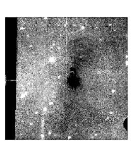
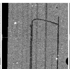
Figure 11: S11 frames after flat correction as an example of memory effects. Left: a negative (dark) area at the center due to a bright star in a previous pointed observation. Right: negative stripes due to one in the all-sky survey together with an arc-like pattern due to one in an FIS slow-scan observation.

4.4 Earthshine light

When the angle between the satellite and the earth became smaller, stray light from the earth appeared in object frames. This is called earthshine light (EL) and is most notable when observing an object around the NEP during summer. The problem is that it is extended but not uniform and that its strength depends on the angular separation of the satellite and the earth limb. When the background sky level changes significantly during one pointed observation, it is most likely due to the EL. Assuming that the EL pattern shape does not change during a pointed observation, Egusa et al. (2013) created a template and successfully removed it from images with a nearby galaxy, i.e. extended object. Tasks for creating and subtracting an EL template are available in the toolkit.

4.5 Drift

The satellite pointing was controlled by two optical telescopes called star trackers installed on the satellite wall. In some observations large drifting took place during an exposure. Although the cause of such large drift is not fully understood yet, we deduce that two possibilities are too few reference stars in the star tracker FoVs and thermal distortion between the telescope axis and the reference frame of the attitude sensors. The PSFs of NIR long exposure frames become very elongated in these cases, since the exposure time is longer than that of MIR. In some extreme cases, the toolkit fails to identify sources used for stacking. While MIR PSFs are not so elongated compared to NIR, the shift values of some frames deviate from the nominal values, and thus such frames are excluded from stacking (§2.3). As already mentioned, this drift mostly occurred in the cross-scan direction.

4.6 Stacking for multiple pointed observations

The current toolkit does not support stacking frames of multiple pointed observations. A user can use the toolkit to produce processed frames before stacking for each pointed observation and then use his/her own code to stack all the processed frames from multiple observations. Note that the central coordinates and rotation angle may differ between observations with the same targetID, i.e. even when the same object was observed with the same AOT.

4.7 Saturation

Bright objects become saturated in long-exposure frames. Such saturated pixels are masked out during the pipeline processing but may be recovered by using the short-exposure frames. However, such a technique has not been established nor implemented in the toolkit.

5 Summary

AKARI is the Japanese infrared astronomical satellite, which performed an all-sky survey and pointed observations with the IRC and the FIS. The IRC is equipped with nine photometric filters covering 2–27 $\mu$m continuously. In this paper, we describe the latest calibration processes for IRC images from pointed observations in Phase 1&2, when the telescope was cooled with liquid Helium. Especially, dark frames, flat frames, calculation schemes of relative shift values, and WCS matching have been improved.

We use the latest toolkit for data reduction to process IRC images from $\sim 4000$ pointed observations during Phase 1&2. Target objects include a wide range of sources from asteroids to distant galaxies. Through the pipeline processing, one stacked image for each filter used in one pointed observation is created. About 90% of the stacked images have a position accuracy better than $1.5^{\prime\prime}$, while this percentage generally decreases with wavelength. Typical sensitivities are estimated to be a factor of $\sim 2$–4 better than AllWISE at similar wavelengths. Remaining artifacts and issues in the processed images are also described.

All of the products including the latest toolkit, processed images, process logs, and Data Users Manual are available via the AKARI Observers website.

The authors fully appreciate a referee’s careful reading of the manuscript and a number of helpful comments and suggestions to improve it.

This work is based on observations with AKARI, a JAXA project with the participation of ESA. The authors greatly appreciate Dr. T. Nakamura for his work on the WCS matching code. The authors also thank Dr. T. Koga, Mr. K. Sano, Mr. S. Koyama, Mr. S. Baba, and Mr. Y. Matsuki for checking the WCS coordinates of stacked images visually. Dr. S. Takita kindly provided the web interface for searching the released data sets.

This research has made use of the VizieR catalogue access tool, CDS, Strasbourg, France. This publication makes use of data products from the Two Micron All Sky Survey, which is a joint project of the University of Massachusetts and the Infrared Processing and Analysis Center/California Institute of Technology, funded by the National Aeronautics and Space Administration and the National Science Foundation, and also from the Wide-field Infrared Survey Explorer, which is a joint project of the University of California, Los Angeles, and the Jet Propulsion Laboratory/California Institute of Technology, funded by the National Aeronautics and Space Administration.

Appendix A Details of released data sets

The processed data together with documents and the latest toolkit was released on 2015 March 31, with a minor update to data on 2015 April 30. All of the products are available via the AKARI observers website. In Table 1, we list a proposal title, 5-digit proposal code, proposal type, and the number of ObsIDs included in this release.

The data package for one ObsID contains neighbor dark frames, a Readme, a log of pipeline processing, and stacked images. The full options adopted during the process are recorded in the log. The Readme file provides a summary for the observation and for the pipeline processing such as the number of frames used for stacking and uncertainties in the WCS matching.

A summary file for all the released ObsIDs is also available. This file lists a summary of information in the Readme for one ObsID per line. Users can overview the whole observations in Phase 1&2 and select ObsIDs that satisfy certain criteria. In addition to a web interface for searching the data sets by object names and coordinates, we provide a list of observations based on the on-sky positions on proposals. The list of proposals is also available online.

Table 1: Title, Proposal ID, type, and the number of ObsIDs for proposal in Phase 1&2

Title	Code	Type†	# of ObsIDs
North Ecliptic Pole Survey	LSNEP	LS	718
Large Magellanic Cloud Survey	LSLMC	LS	598
Evolution of Cluster of Galaxies	CLEVL	MP	278
Interstellar dust and gas in various environments of our Galaxy and nearby galaxies	ISMGN	MP	260
ASTRO-F Studies on Star formation and Star forming regions	AFSAS	MP	237
DT for IRC	DTIRC	DT	224
Debris Disks Around Main Sequence Stars and Extra-solar Zodiacal Emissions	VEGAD	MP	197
Origin and Evolution of Solar System Objects	SOSOS	MP	157
Unbiased Slit-Less Spectroscopic Survey of Galaxies	SPICY	MP	140
Astro-F Ultra-Deep Imaging/Spectroscopy of the Spitzer/IRAC Dark Field	EGAMI	OT	87
Mass loss and stellar evolution in the AGB phase	AGBGA	MP	81
Evolution of ULIRGs and AGNs	AGNUL	MP	65
Understanding the Dust Properties of Elliptical Galaxies	EGALS	OT	52
FUHYU - SPITZER WELL STUDIED FIELD MISSION PROGRAM	FUHYU	MP	50
Making AGN come of age as cosmological probes	6AND7	OT	50
The Nature of New ULIRGs at intermediate redshift	NULIZ	OT	48
NIR–MIR Spectroscopic Survey of Selected Areas in the Galactic Plane	SPECS	OT	47
The spatial distribution of ices in Spitzer-selected molecular cores	IMAPE	OT	46
PV for IRC	PVIRC	DT	43
Astro-F Spectroscopic Observation of $z=6$ QSOs	HZQSO	OT	43
Search for Giant Planets around White Dwarfs	SGPWD	OT	41
Deep IR Imaging of the Unique NEP Cluster at $z=0.813$	CLNEP	OT	38
15 Micron Imaging of Extended Groth Strip	GROTH	OT	31
Formation and Evolution of Interstellar Ice	ISICE	OT	30
Dust, PAHs and molecules in molecular clouds	CERN2	OT	28
UV-selected Lyman Break Galaxies at $0.6<z<1.3$ in the Spitzer FLS	Z1LBG	OT	27
Mid-Infrared Imaging of the ASTRO-F Deep SEP Field	IRSEP	OT	26
Mapping the Spectral Energy Distributions of Sub-mm Bright QSOs	SUBMM	OT	22
Extreme Colors: The smoking Gun of Dust Aggregation and Fragmentation	COLVN	OT	21
An ultra-deep survey through a well-constrained lensing cluster	A2218	OT	19
IRC NIR Spectroscopy of High-Redshift Quasars	NSPHQ	OT	16
Cool Dust in the Environments of Evolved Massive Stars	WRENV	OT	15
Near Infrared Spectroscopy of L and T Dwarfs	NIRLT	MP	15
DT for FIS	DTFIS	DT	13
Triggered massive-star formation in the Galaxy	AZTSF	OT	13
The role of pulsation in mass loss along the Asymptotic Giant Branch	SMCPM	OT	12
Dust and gas properties in AGB and post-AGB objects	CERN1	OT	12
Evolution of dust and gas in Photodissociation Regions	DGPDR	OT	11
Activity of Small Solar System Bodies far from the Sun	ADAMB	OT	11
Deep Extinction Maps of Dense Cores	DEMDC	OT	10
Stars departing from the Asymptotic Giant Branch	DEAGB	OT	10
Probing molecular tori n Obscured AGN through CO Absorption	COABS	OT	10
A Search for Very Low Luminosity Objects in Dense Molecular Cores	VELLO	OT	9
Search for Emission Outside the Disks of Edge-on Galaxies	HALOS	OT	9
Accretion and protoplanetary disks in brown dwarfs	DISKB	OT	8
The hidden evolution from AGB stars to PNe as seen by ASTRO-F/IRC	AGBPN	OT	8
ASTRO-F/IRC Slit-less Spectroscopy of Hickson Compact Groups	SHARP	OT	7
Far-infrared Emission from the Coma Cluster of Galaxies	FIREC	OT	7
Far-Infrared Spectroscopic Observation of Eta Carinae	ETASP	OT	7
Excavating Mass Loss History in Extended Dust Shells of Evolved Stars	MLHES	MP	5
Calibrating mid-IR dust attenuation tracers for LBGs with ASTRO-F	IRLBG	OT	5
Dusty Star-Formation History of the Universe	GALEV	MP	5
Spectroscopic Search for Atmosphere of an Extra-Solar Planet	EXOSP	OT	4
The stellar mass and the obscured star formation harboured by EROs	EROMU	OT	4
15 Micron Imaging of the $z=2.38$ Filament	BLOBS	OT	4
FIR Spectroscopy of Super Nova Remnants	SNRBS	OT	3
Star Formation and Environment in the COSMOS Field	COSMS	OT	3
Near-Infrared Spectroscopy of the Atmospheres of Uranus and Neptune	UNIRC	OT	2
The Nature of the Dusty Medium in Dwarf Elliptical Galaxies	DUDES	OT	2
$\dagger$: LS=Large Survey, MP=Mission Program, OT=Open Time, DT=Director’s Time

Appendix B Details of the all-data processing

B.1 Relative shift between frames

Histograms of relative shift in the x- and y-direction for each dithering cycle in the case of IRC02 and IRC03 are presented in Figure 13. For the rotation angle, a histogram is created using the data from all dithering cycles (Figure 13). As with the case for IRC00 and IRC05 (Figure 8), shift values are for MIR-S frames after the sub-pixel sampling and the lower and upper limits adopted in the toolkit are indicated by blue dashed lines. The wings in histograms of the x-direction shift found in the IRC00 and IRC05 cases are also seen in Figure 13.

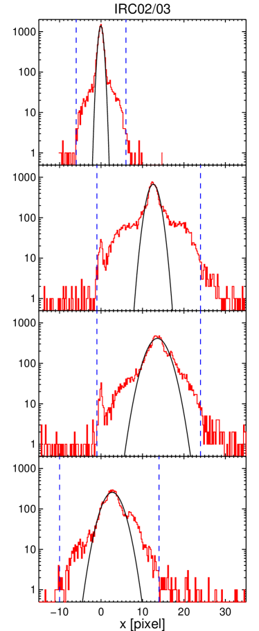
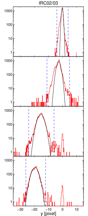
Figure 12: Histogram of relative shift in x- (left) and y-direction (right) of MIR-S frames for each dithering cycle (from top to bottom) of IRC02 and IRC03. Pixel numbers are after the sub-pixel sampling, i.e. twice the original value. One pixel is $1.17^{\prime\prime}$ for MIR-S. Black curves represent the results of gaussian fit to the histogram and blue dashed lines indicate the lower and upper limits adopted in the toolkit.

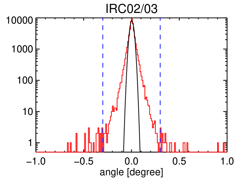
Figure 13: Histogram of rotation angle of MIR-S frames for IRC02 and IRC03. Black curves represent the results of gaussian fit to the histogram and blue dashed lines indicate the lower and upper limits adopted in the toolkit.

B.2 Accuracy of WCS matching

The residual of WCS matching is recorded as a FITS header parameter ‘WCSERROR’. This is a root-mean-square of positional offsets between matched WCS and catalogued WCS for sources in a stacked image. A histogram of this value for each filter is presented in Figure 14. Since the tolerance for WCS matching is set to be $1.5^{\prime\prime}$, the residual is smaller than this limit. If the residual becomes larger than this limit, that WCS matching is considered as being failed.

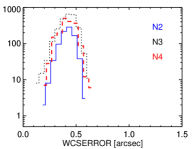
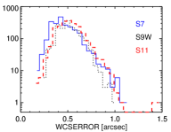
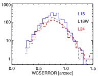
Figure 14: Histogram of residuals of the WCS matching for NIR (left), MIR-S (middle), and MIR-L (right).

B.3 Sensitivity variation

As explained in §3.3, we measure the sky standard deviation $\sigma$ of stacked images from pointed observations toward the NEP region. For each month, AOT, and filter, we pick one pointed observation that has the largest number of stacked frames and measure $\sigma$. In Figure 15, the temporal variation of $\sigma$ values is presented for the whole Phase 1&2. We here note again that these values are measured in stacked images with sub-pixel sampling. Large $\sigma$ values during May and July at longer wavelengths are primarily due to the Earthshine light (§4.4). Therefore, we measure typical values of $\sigma$ (listed in Table 3.3) from data taken between 2006 August and 2007 April.

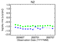
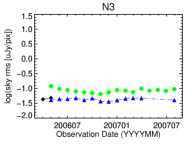
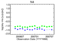
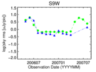
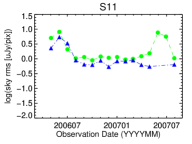
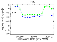
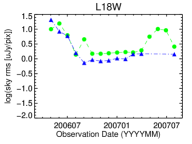
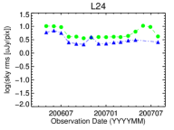
Figure 15: Temporal variation of sky standard deviation from NEP observations. Different symbols indicate different AOTs: black diamond for IRC00, green circle for IRC03, and blue triangle for IRC05.

B.4 Typical PSF sizes

In order to estimate PSF sizes of processed images, we performed a 2D gaussian fit to sources found in stacked images of NEP observations taken during 2006 October and 2006 December. Histograms of measured sizes (major and minor axis lengths in FWHM of the fitted 2D gaussian) were created for each filter and each AOT (Figure 16). Then a gaussian profile was fitted to each histogram and its peak position is adopted as a typical PSF size (Table 3.4). During the fit, we manually set the lower limit of PSF sizes in order to exclude histogram peaks due to noises (especially in NIR of IRC03) and sub-peaks of PSFs (especially in L24). Widths of histograms and thus of fitted gaussian vary, but are typically $0.2^{\prime\prime}$–$0.5^{\prime\prime}$.

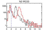
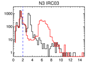
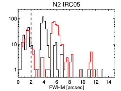
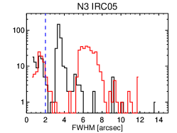
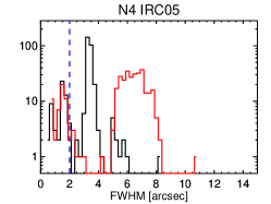
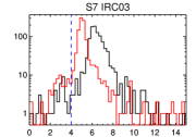
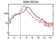
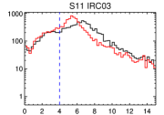
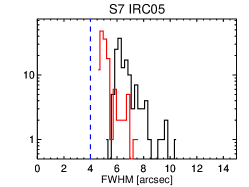
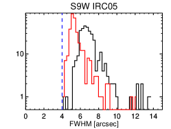
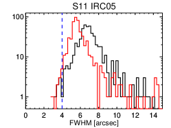
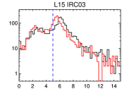
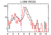
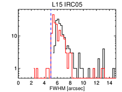
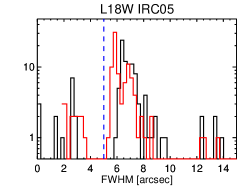
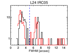
Figure 16: Histogram of PSF sizes of stacked images from NEP observations during 2006 October–December. FWHM [arcsec] along the major and minor axes of fitted 2D gaussian is presented. Black and red lines indicate the length of axis closer to x- and y-directions of the stacked images, respectively. Blue dashed lines indicate the lower limit adopted when fitting a gaussian to the histogram to estimate the typical PSF sizes listed in Table 3.4.

In Figure 16, the black line corresponds to the length of axis closer to the x-axis of stacked images, while the red line corresponds to the one closer to the y-axis. For NIR, the peak of red histograms (i.e. the PSF size roughly along the y-axis) is always at larger values compared to that of black histograms. For MIR, the trend is reversed, i.e. that of black histograms is at larger values, although the difference is smaller than in the NIR cases. In summary, the NIR PSF is more elongated along the y-axis while the MIR PSF is slightly elongated along the x-axis. Considering the FoV alignment (Figure 1), both of these axes correspond to the cross-scan direction, which indicates that the effect of drift is more significant in this direction. This is consistent with the wings seen in histograms of relative shift values in the x-axis direction of MIR-S images (Figures 8 and 13).

References

- Arimatsu et al. (2011a) Arimatsu, K., Izumiura, H., Ueta, T., Yamamura, I., & Onaka, T. 2011a, ApJ, 729, L19
- Arimatsu et al. (2011b) Arimatsu, K., et al. 2011b, PASP, 123, 981
- Cohen (2003) Cohen, M. 2003, in ESA Special Publication, Vol. 481, The Calibration Legacy of the ISO Mission, ed. L. Metcalfe, A. Salama, S. B. Peschke, & M. F. Kessler, 135
- Cohen et al. (2003a) Cohen, M., Megeath, S. T., Hammersley, P. L., Martín-Luis, F., & Stauffer, J. 2003a, AJ, 125, 2645
- Cohen et al. (1999) Cohen, M., Walker, R. G., Carter, B., Hammersley, P., Kidger, M., & Noguchi, K. 1999, AJ, 117, 1864
- Cohen et al. (2003b) Cohen, M., Wheaton, W. A., & Megeath, S. T. 2003b, AJ, 126, 1090
- Cohen et al. (1996) Cohen, M., Witteborn, F. C., Carbon, D. F., Davies, J. K., Wooden, D. H., & Bregman, J. D. 1996, AJ, 112, 2274
- Condon (1974) Condon, J. J. 1974, ApJ, 188, 279
- Egusa et al. (2013) Egusa, F., Wada, T., Sakon, I., Onaka, T., Arimatsu, K., & Matsuhara, H. 2013, ApJ, 778, 1
- Hasegawa et al. (2008) Hasegawa, S., et al. 2008, PASJ, 60, 399
- Hogg (2001) Hogg, D. W. 2001, AJ, 121, 1207
- Ita et al. (2007) Ita, Y., et al. 2007, PASJ, 59, 437
- Ita et al. (2008) —. 2008, PASJ, 60, 435
- Kaneda et al. (2008) Kaneda, H., Suzuki, T., Onaka, T., Okada, Y., & Sakon, I. 2008, PASJ, 60, 467
- Kato et al. (2012) Kato, D., et al. 2012, AJ, 144, 179
- Kawada et al. (2007) Kawada, M., et al. 2007, PASJ, 59, 389
- Lee et al. (2009) Lee, H. M., et al. 2009, PASJ, 61, 375
- Matsuhara et al. (2006) Matsuhara, H., et al. 2006, PASJ, 58, 673
- Mori et al. (2012) Mori, T. I., Sakon, I., Onaka, T., Kaneda, H., Umehata, H., & Ohsawa, R. 2012, ApJ, 744, 68
- Müller et al. (2014) Müller, T. G., Hasegawa, S., & Usui, F. 2014, PASJ, 66, 52
- Murakami et al. (2007) Murakami, H., et al. 2007, PASJ, 59, 369
- Murata et al. (2013) Murata, K., et al. 2013, A&A, 559, A132
- Onaka et al. (2007) Onaka, T., et al. 2007, PASJ, 59, 401
- Onaka et al. (2010) Onaka, T., et al. 2010, in Society of Photo-Optical Instrumentation Engineers (SPIE) Conference Series, Vol. 7731, Society of Photo-Optical Instrumentation Engineers (SPIE) Conference Series, 0
- Pearson et al. (2010) Pearson, C. P., et al. 2010, A&A, 514, A9
- Sakon et al. (2007) Sakon, I., et al. 2007, PASJ, 59, 483
- Scoville et al. (2007) Scoville, N., et al. 2007, ApJS, 172, 1
- Shimonishi et al. (2013) Shimonishi, T., Onaka, T., Kato, D., Sakon, I., Ita, Y., Kawamura, A., & Kaneda, H. 2013, AJ, 145, 32
- Skrutskie et al. (2006) Skrutskie, M. F., et al. 2006, AJ, 131, 1163
- Takagi et al. (2010) Takagi, T., et al. 2010, A&A, 514, A5
- Tanabé et al. (2008) Tanabé, T., et al. 2008, PASJ, 60, 375
- Tsumura & Wada (2011) Tsumura, K., & Wada, T. 2011, PASJ, 63, 755
- Wada et al. (2008) Wada, T., et al. 2008, PASJ, 60, 517
- Wright et al. (2010) Wright, E. L., et al. 2010, AJ, 140, 1868
- Yamagishi et al. (2010) Yamagishi, M., Kaneda, H., Ishihara, D., Komugi, S., Suzuki, T., & Onaka, T. 2010, PASJ, 62, 1085