Morpho-syntactic Lexicon Generation
Using Graph-based Semi-supervised Learning

Abstract

Morpho-syntactic lexicons provide information about the morphological and syntactic roles of words in a language. Such lexicons are not available for all languages and even when available, their coverage can be limited. We present a graph-based semi-supervised learning method that uses the morphological, syntactic and semantic relations between words to automatically construct wide coverage lexicons from small seed sets. Our method is language-independent, and we show that we can expand a 1000 word seed lexicon to more than 100 times its size with high quality for 11 languages. In addition, the automatically created lexicons provide features that improve performance in two downstream tasks: morphological tagging and dependency parsing.

1 Introduction

Morpho-syntactic lexicons contain information about the morphological attributes and syntactic roles of words in a given language. A typical lexicon contains all possible attributes that can be displayed by a word. Table 1 shows some entries in a sample English morpho-syntactic lexicon. As these lexicons contain rich linguistic information, they are useful as features in downstream NLP tasks like machine translation [Nießen and Ney, 2004, Minkov et al., 2007, Green and DeNero, 2012], part of speech tagging [Schmid, 1994, Denis and Sagot, 2009, Moore, 2015], dependency parsing [Goldberg et al., 2009], language modeling [Arisoy et al., 2010] and morphological tagging [Müller and Schuetze, 2015] inter alia. There are three major factors that limit the use of such lexicons in real world applications: (1) They are often constructed manually and are expensive to obtain [Kokkinakis et al., 2000, Dukes and Habash, 2010]; (2) They are currently available for only a few languages; and (3) Size of available lexicons is generally small.

played	POS:Verb, Tense:Past, VForm:Fin, $\dots$
playing	POS:Verb, Tense:Pres, VForm:Ger, $\dots$
awesome	POS:Adj, Degree:Pos

Table 1: A sample English morpho-syntactic lexicon.

In this paper, we present a method that takes as input a small seed lexicon, containing a few thousand annotated words, and outputs an automatically constructed lexicon which contains morpho-syntactic attributes (henceforth referred to as attributes) for a large number of words of a given language. We model the problem of morpho-syntactic lexicon generation as a graph-based semi-supervised learning problem [Zhu, 2005, Bengio et al., 2006, Subramanya and Talukdar, 2014]. We construct a graph where nodes represent word types and the goal is to label them with attributes. The seed lexicon provides attributes for a subset of these nodes. Nodes are connected to each other through edges that denote features shared between them or surface morphological transformation between them.

Our entire framework of lexicon generation, including the label propagation algorithm and the feature extraction module is language independent. We only use word-level morphological, semantic and syntactic relations between words that can be induced from unannotated corpora in an unsupervised manner. One particularly novel aspect of our graph-based framework is that edges are featurized. Some of these features measure similarity, e.g., singular nouns tend to occur in similar distributional contexts as other singular nouns, but some also measure transformations from one inflection to another, e.g., adding a ‘s’ suffix could indicate flipping the Num:Sing attribute to Num:Plur (in English). For every attribute to be propagated, we learn weights over features on the edges separately. This is in contrast to traditional label propagation, where edges indicate similarity exclusively [Zhu, 2005].

We construct lexicons in 11 languages of varying morphological complexity. We perform intrinsic evaluation of the quality of generated lexicons obtained from either the universal dependency treebank or created manually by humans (§4). We show that these automatically created lexicons provide useful features in two extrinsic NLP tasks which require identifying the contextually plausible morphological and syntactic roles: morphological tagging [Hajič and Hladká, 1998, Hajič, 2000] and syntactic dependency parsing [Kübler et al., 2009]. We obtain an average of 15.4% and 5.3% error reduction across 11 languages for morphological tagging and dependency parsing respectively on a set of publicly available treebanks (§5). We anticipate that the lexicons thus created will be useful in a variety of NLP problems.

2 Graph Construction

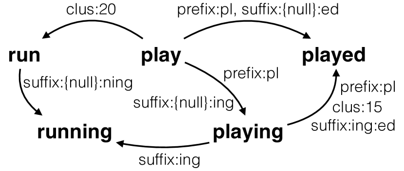
Figure 1: A subgraph from the complete graph of English showing different kinds of features shared on the edges between words. Some possible features/edges have been removed for enhancing clarity.

The approach we take propagates information over lexical graphs (§3). In this section we describe how to construct the graph that serves as the backbone of our model. We construct a graph in which nodes are word types and directed edges are present between nodes that share one or more features. Edges between nodes denote that there might be a relationship between the attributes of the two nodes, which we intend to learn. As we want to keep our model language independent, we use edge features that can be induced between words without using any language specific tools. To this end, we describe three features in this section that can be obtained using unlabeled corpora for any given language. Fig. 1 shows a subgraph of the full graph constructed for English.

Word Clusters.

Previous work has shown that unlabeled text can be used to induce unsupervised word clusters which can improve the performance of many NLP tasks in different languages [Clark, 2003, Koo et al., 2008, Turian et al., 2010, Faruqui and Padó, 2010, Täckström et al., 2012, Owoputi et al., 2013]. Word clusters capture semantic and syntactic similarities between words, for example, play and run are present in the same cluster. We obtain word clusters by using Exchange clustering algorithm [Kneser and Ney, 1993, Martin et al., 1998, Uszkoreit and Brants, 2008] on large unlabeled corpus of every language. As in ?), we use one year of news articles scrapped from a variety of sources and cluster only the most frequent 1M words into 256 different clusters. An edge was introduced for every word pair sharing the same word cluster and a feature for the cluster is fired. Thus, there are 256 possible cluster features on an edge, though in our case only a single one can fire.

Suffix & Prefix.

Suffixes are often strong indicators of the morpho-syntactic attributes of a word [Ratnaparkhi, 1996, Clark, 2003]. For example, in English, -ing denotes gerund verb forms like, studying, playing and -ed denotes past tense like studied, played etc. Prefixes like un-, in- often denote adjectives. Thus we include both 2-gram and 3-gram suffix and prefix as edge features. We introduce an edge between two words sharing a particular suffix or prefix feature.

Morphological Transformations.

?) presented an unsupervised method of inducing prefix- and suffix-based morphological transformations between words using word embeddings. In their method, statistically, most of the transformations are induced between words with the same lemma (without using any prior information about the word lemma). For example, their method induces the transformation between played and playing as suffix:ed:ing. This feature indicates Tense:Past to turn off and Tense:Pres to turn on. We train the morphological transformation prediction tool of ?) on the news corpus (same as the one used for training word clusters) for each language. An edge is introduced between two words that exhibit a morphological transformation feature from one word to another as indicated by the tool’s output.

Motivation for the Model.

To motivate our model, consider the words played and playing. They have a common attribute POS:Verb but they differ in tense, showing Tense:Past and Tense:Pres resp. Typical graph-propagation algorithms model similarity [Zhu, 2005] and thus propagate all attributes along the edges. However, we want to model if an attribute should propagate or change across an edge. For example, having a shared cluster feature, is an indication of similar POS tag [Clark, 2003, Koo et al., 2008, Turian et al., 2010], but a surface morphological transformation feature like suffix:ed:ing possibly indicates a change in the tense of the word. Thus, we will model attributes propagation/transformation as a function of the features shared on the edges between words. The features described in this section are specially suitable for languages that exhibit concatenative morphology, like English, German, Greek etc. and might not work very well with languages that exhibit non-concatenative morphology i.e, where root modification is highly frequent like in Arabic and Hebrew. However, it is important to note that our framework is not limited to just the features described here, but can incorporate any arbitrary information over word pairs (§8).

3 Graph-based Label Propagation

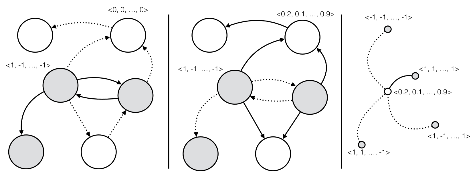
Figure 2: Word graph with edges between words showing the labeled (grey) and the unlabeled (white) word nodes. Only nodes connected via solid edges are visible to each other, dotted edges block visibility. This figure demonstrates interaction between nodes during model estimation (left), label propagation (center), and paradigm projection (right). Attribute-value vectors of the words are shown in angled brackets. The solid edge in the right figure shows the closest attribute paradigm to which the empirical vector is projected.

We now describe our model. Let $\mathcal{W}=\{w_{1},w_{2},\ldots,w_{|\mathcal{W}|}\}$ be the vocabulary with $|\mathcal{W}|$ words and $\mathcal{A}=\{a_{1},a_{2},\ldots,a_{|\mathcal{A}|}\}$ be the set of lexical attributes that words in $\mathcal{W}$ can express; e.g. $\mathcal{W}=\{played,playing,\ldots\}$ and $\mathcal{A}=\{\textsc{Num:Sing},\textsc{Num:Plur},\textsc{Tense:Past},\ldots\}$. Each word type $w\in\mathcal{W}$ is associated with a vector $\mathbf{a}_{w}\in[-1,1]^{|\mathcal{A}|}$, where $a_{i,w}=1$ indicates that word $w$ has attribute $i$ and $a_{i,w}=-1$ indicates its absence; values in between are treated as degrees of uncertainty. For example, $\textsc{Tense:Past}_{played}=1$ and $\textsc{Tense:Past}_{playing}=-1$.

The vocabulary $\mathcal{W}$ is divided into two disjoint subsets, the labeled words $\mathcal{L}$ for which we know their $\mathbf{a}_{w}$’s (obtained from seed lexicon) and the unlabeled words $\mathcal{U}$ whose attributes are unknown. In general $|\mathcal{U}|\gg|\mathcal{L}|$. The words in $\mathcal{W}$ are organized into a directed graph with edges $\mathcal{E}$ between words. Let, vector $\boldsymbol{\phi}(w,v)\in[0,1]^{|\mathcal{F}|}$ denote the features on the directed edge between words $w$ and $v$, with $1$ indicating the presence and $0$ the absence of feature $f_{k}\in\mathcal{F}$, where, $\mathcal{F}=\{f_{1},f_{2},\ldots,f_{|\mathcal{F}|}\}$ are the set of possible binary features shared between two words in the graph. For example, the features on edges between played and playing from Fig. 1 are:

$$\phi_{k}(played,playing)=\begin{cases}1,&\text{if}f_{k}=\text{suffix:ed:ing}\\ 1,&\text{if}f_{k}=\text{prefix:pl}\\ 0,&\text{if}f_{k}=\text{suffix:ly}\\ \dots\end{cases}$$

We seek to determine which subsets of $\mathcal{A}$ are valid for each word $w\in\mathcal{W}$. We learn how a particular attribute of a node is a function of that particular attribute of its neighboring nodes and features on the edge connecting them. Let $a_{i,w}$ be an attribute of word $w$ and let $\hat{a}_{i,w}$ be the empirical estimate of that attribute. We posit that $\hat{a}_{i,w}$ can be estimated from the neighbors $\mathcal{N}(w)$ of $w$ as follows:

$$\hat{a}_{i,w}=\mathrm{tanh}\left(\sum_{v\in\mathcal{N}(w)}\left(\boldsymbol{\phi}(w,v)\cdot\boldsymbol{\theta_{i}}\right)\times a_{i,v}\right)$$ (1)

where, $\boldsymbol{\theta_{i}}\in\mathbb{R}^{|\mathcal{F}|}$ is weight vector of the edge features for estimating attribute $a_{i}$. ‘$\cdot$’ represents dot product betwen two vectors. We use tanh as the non-linearity to make sure that $\hat{a}_{i,w}\in[-1,1]$. The set of such weights $\boldsymbol{\theta}\in\mathbb{R}^{|\mathcal{A}|\times|\mathcal{F}|}$ for all attributes are the model parameters that we learn. Our graph resembles the Ising model, which is a lattice model proposed for describing intermolecular forces [Ising, 1925], and eq. 1 solves the naive mean field approximation of the Ising model [Wang et al., 2007].

Intuitively, one can view the node to node message function from $v$ to $w$: $\boldsymbol{\phi}(w,v)\cdot\boldsymbol{\theta_{i}}\times a_{i,v}$ as either (1) supporting the value $a_{i,v}$ when $\boldsymbol{\phi}(w,v)\cdot\boldsymbol{\theta_{i}}>0$; (2) inverting $a_{i,v}$ when $\boldsymbol{\phi}(w,v)\cdot\boldsymbol{\theta_{i}}<0$; or (3) dampening or neutering $a_{i,v}$ when $\boldsymbol{\phi}(w,v)\cdot\boldsymbol{\theta_{i}}\approx 0$. Returning to our motivation, if $w=played$ and $v=playing$, a feature indicating the suffix substitution suffix:ed:ing should have a highly negative weight for Tense:Past, indicating a change in value. This is because Tense:Past = -1 for playing, and a negative value of $\boldsymbol{\phi}(w,v)\cdot\boldsymbol{\theta_{i}}$ will push it to positive for played.

It should be noted that this framework for constructing lexicons does not explicitly distinguish between morpho-syntactic paradigms, but simply identifies all possible attribute-values a word can take. If we consider an example like “games” and two attributes, the syntactic part-of-speech, POS, and number, Num, games can either be 1) $\{\textsc{POS:Verb},\textsc{Num:Sing}\}$, as in John games the system; or $\{\textsc{POS:Noun},\textsc{Num:Plur}\}$, as in The games have started. Our framework will mereley return that all the above attribute-values are possible, which implies that the singluar noun and plural verb interpretations are valid. One possible way to account for this is to make full morphological paradigms the “attributes” in or model. But this leads to slower runtimes and sparser learning. We leave as future work extensions to full paradigm prediction.

Our framework has three critical components, each described below: (1) model estimation, i.e., learning $\boldsymbol{\theta}$; (2) label propagation to $\mathcal{U}$; and optionally (3) paradigm projection to known valid morphological paradigms. The overall procedure is illustrated in Figure 2 and made concrete in Algorithm 1.

Data: $\mathcal{W}$, $\mathcal{L}$, $\mathcal{U}$, $\mathcal{A}$, $\mathcal{F}$, $\mathcal{P}$

Result: $\boldsymbol{\theta}$, labeled $\mathcal{U}$

// model estimation

1 while not convergence do

2       for $w\in\mathcal{L}$ do

3             loss $\leftarrow\|\mathbf{a}_{w}-\hat{\mathbf{a}}_{w}\|_{2}^{2}$

4             Update $\boldsymbol{\theta}$ using $\frac{\partial\mathrm{loss}}{\partial\boldsymbol{\theta}}$

5            

6      

// label propagation

7 while not convergence do

8       for $w\in\mathcal{U}$ do

9             $\mathbf{a}_{w}\leftarrow\hat{\mathbf{a}}_{w}$

10            

11      

// paradigm projection

12 for $w\in\mathcal{U}$ do

13       mindist $\leftarrow\infty$, closest $\leftarrow\emptyset$

14       for $\mathbf{p}\in\mathcal{P}$ do

15             dist $\leftarrow\|\mathbf{a}_{w}-\mathbf{p}\|_{2}^{2}$

16             if dist $<$ mindist then

17                   mindist $\leftarrow$ dist, closest $\leftarrow\mathbf{p}$

18                  

19            

20       $\mathbf{a}_{w}\leftarrow$ closest

21      

Algorithm 1 Graph-based semi-supervised label propagation algorithm.

3.1 Model Estimation

We estimate all individual elements of an attribute vector using eq. 1. We define loss as the squared loss between the empirical and observed attribute vectors on every labeled node in the graph, thus the total loss can be computed as:

$$\sum_{w\in\mathcal{L}}\|\mathbf{a}_{w}-\hat{\mathbf{a}}_{w}\|_{2}^{2}$$ (2)

We train the edge feature weights $\boldsymbol{\theta}$ by minimizing the loss function in eq. 2. In this step, we only use labeled nodes and the edge connections between labeled nodes. As such, this is strictly a supervised learning setup. We minimize the loss function using online adaptive gradient descent [Duchi et al., 2011] with $\ell_{2}$ regularization on the feature weights $\boldsymbol{\theta}$. This is the first step in Algorithm 1 (lines 1–4).

3.2 Label Propagation

In the second step, we use the learned weights of the edge features to estimate the attribute values over unlabeled nodes iteratively. The attribute vector of all unlabeled words is initialized to null, $\forall w\in\mathcal{U},\mathbf{a}_{w}=\langle 0,0,\ldots,0\rangle$. In every iteration, an unlabeled node estimates its empirical attributes by looking at the corresponding attributes of its labeled and unlabeled neighbors using eq. 1, thus this is the semi-supervised step. We stop after the squared euclidean distance between the attribute vectors at two consecutive iterations for a node becomes less than 0.1 (averaged over all unlabeled nodes). This is the second step in Algorithm 1 (lines 5–7). After convergence, we can directly obtain attributes for a word by thresholding: a word $w$ is said to possess an attribute $a_{i}$ if $a_{i,w}>0$.

3.3 Paradigm Projection

Since a word can be labeled with multiple lexical attributes, this is a multi-label classification problem. For such a task, several advanced methods that take into account the correlation between attributes have been proposed [Ghamrawi and McCallum, 2005, Tsoumakas and Katakis, 2006, Fürnkranz et al., 2008, Read et al., 2011], here we have adopted the binary relevance method which trains a classifier for every attribute independently of the other attributes, for its simplicity [Godbole and Sarawagi, 2004, Zhang and Zhou, 2005].

However, as the decision for the presence of an attribute over a word is independent of all the other attributes, the final set of attributes obtained for a word in §3.2 might not be a valid paradigm. For example, a word cannot only exhibit the two attributes POS:Noun and Tense:Past, since the presence of the tense attribute implies POS:Verb should also be true. Further, we want to utilize the inherent correlations between attribute labels to obtain better solutions. We thus present an alternative, simpler method to account for this problem. To ensure that we obtain a valid attribute paradigm, we project the empirical attribute vector obtained after propagation to the space of all valid paradigms.

We first collect all observed and thus valid attribute paradigms from the seed lexicon ($\mathcal{P}=\{\mathbf{a}_{w}|w\in\mathcal{L}\}$). We replace the empirical attribute vector obtained in §3.2 by a valid attribute paradigm vector which is nearest to it according to euclidean distance. This projection step is inspired from the decoding step in label-space transformation approaches to multilabel classification [Hsu et al., 2009, Ferng and Lin, 2011, Zhang and Schneider, 2011]. This is the last step in Algorithm 1 (lines 8–14). We investigate for each language if paradigm projection is helpful (§4.1).

4 Intrinsic Evaluation

	$|\mathcal{L}|$	$|\mathcal{W}|$	$|\mathcal{E}|$	$|\mathcal{A}|$	$|\mathcal{P}|$	Prop
	(k)	(k)	(m)			(k)
eu	3.4	130	13	83	811	118
bg	8.1	309	27	57	53	285
hr	6.9	253	26	51	862	251
cs	58.5	507	51	122	4,789	403
da	5.9	259	26	61	352	246
en	4.1	1,006	100	50	412	976
fi	14.4	372	30	100	2,025	251
el	3.9	358	26	40	409	236
hu	1.9	451	25	85	490	245
it	8.5	510	28	52	568	239
sv	4.8	305	26	41	265	268

Table 2: Graph statistics for different languages, showing the approximate number of labeled seed nodes ($|\mathcal{L}|$), labeled and unlabeled nodes ($|\mathcal{W}|$), edges between words ($|\mathcal{E}|$), the number of unique attributes ($|\mathcal{A}|$), attribute paradigms ($|\mathcal{P}|$) and size of the constructed lexicon (Prop). k: thousands, m: millions.

To ascertain how our graph-propagation framework predicts morphological attributes for words, we provide an intrinsic evaluation where we compare predicted attributes to gold lexicons that have been either read off from a treebank or derived manually.

4.1 Dependency Treebank Lexicons

The universal dependency treebank [McDonald et al., 2013, De Marneffe et al., 2014, Agić et al., 2015] contains dependency annotations for sentences and morpho-syntactic annotations for words in context for a number of languages. A word can display different attributes depending on its role in a sentence. In order to create morpho-syntactic lexicon for every language, we take the union of all the attributes that the word realizes in the entire treebank. Although, it is possible that this lexicon might not contain all realizable attributes if a particular attribute or paradigm is not seen in the treebank (we address this issue in §4.2). The utility of evaluating against treebank derived lexicons is that it allows us to evaluate on a large set of languages. In particular, in the universal dependency treebanks v1.1 [Agić et al., 2015], 11 diverse languages contain the morphology layer, including Romance, Germanic and Slavic languages plus isolates like Basque and Greek.

We use the train/dev/test set of the treebank to create training (seed), development and test lexicons for each language. We exclude words from the dev and test lexicon that have been seen in seed lexicon. For every language, we create a graph with the features described in §2 with words in the seed lexicon as labeled nodes. The words from development and test set are included as unlabeled nodes for the propagation stage. Table 2 shows statistics about the constructed graph for different languages.

We perform feature selection and hyperparameter tuning by optimizing prediction on words in the development lexicon and then report results on the test lexicon. The decision whether paradigm projection (§3.3) is useful or not is also taken by tuning performance on the development lexicon. Table 3 shows the features that were selected for each language. Now, for every word in the test lexicon we obtain predicted lexical attributes from the graph. For a given attribute, we count the number of words for which it was correctly predicted (true positive), wrongly predicted (false positive) and not predicted (false negative). Aggregating these counts over all attributes ($\mathcal{A}$), we compute the micro-averaged $F_{1}$ score and achieve 74.3% on an average across 11 languages (cf. Table 4). Note that this systematically underestimates performance due to the effect of missing attributes/paradigms that were not observed in the treebank.

Propagated Lexicons.

The last column in Table 2 shows the number of words in the propagated lexicon, and the first column shows the number of words in the seed lexicon. The ratio of the size of propagated and seed lexicon is different across languages, which presumably depends on how densely connected each language’s graph is. For example, for English the propagated lexicon is around $240$ times larger than the seed lexicon, whereas for Czech, its $8$ times larger. We can individually tune how densely connected graph we want for each language depending on the seed size and feature sparsity, which we leave for future work.

Selected Edge Features.

The features most frequently selected across all the languages are the word cluster and the surface morphological transformation features. This essentially translates to having a graph that consists of small connected components of words having the same lemma (discovered in an unsupervised manner) with semantic links connecting such components using word cluster features. Suffix features are useful for highly inflected languages like Czech and Greek, while the prefix feature is only useful for Czech. Overall, the selected edge features for different languages correspond well to the morphological structure of these languages [Dryer, 2013].

	Clus	Suffix	Prefix	MorphTrans	Proj
eu	✓			✓	✓
bg	✓			✓
hr	✓	✓			✓
cs	✓	✓	✓	✓	✓
da	✓			✓	✓
en	✓			✓	✓
fi	✓			✓
el	✓	✓		✓	✓
hu	✓			✓	✓
it	✓			✓	✓
sv	✓	✓			✓

Table 3: Features selected and the decision of paradigm projection (Proj) tuned on the development lexicon for each language. ✓denotes a selected feature.

Corpus Baseline.

We compare our results to a corpus-based method of obtaining morpho-syntactic lexicons. We hypothesize that if we use a morphological tagger of reasonable quality to tag the entire wikipedia corpus of a language and take the union of all the attributes for a word type across all its occurrences in the corpus, then we can acquire all possible attributes for a given word. Hence, producing a lexicon of reasonable quality. ?) used this technique to obtain a high quality tag dictionary for POS-tagging. We thus train a morphological tagger (detail in §5.1) on the training portion of the dependency treebank and use it to tag the entire wikipedia corpus. For every word, we add an attribute to the lexicon if it has been seen at least $k$ times for the word in the corpus, where $k\in[2,20]$. This threshold on the frequency of the word-attribute pair helps prevent noisy judgements. We tune $k$ for each language on the development set and report results on the test set in Table 4. We call this method the Corpus baseline. It can be seen that for every language we outperform this baseline, which on average has an $F_{1}$ score of 67.1%.

	words	Corpus	Propagation
eu	3409	54.0	57.5
bg	2453	66.4	73.6
hr	1054	69.7	71.6
cs	14532	79.1	80.8
da	1059	68.2	78.1
en	3142	57.2	72.0
fi	2481	58.2	68.2
el	1093	72.2	82.4
hu	1004	64.9	70.9
it	1244	78.8	81.7
sv	3134	69.8	80.7
avg.	3146	67.1	74.3

Table 4: Micro-averaged $F_{1}$ score (%) for prediction of lexical attributes on the test set using our propagation algorithm (Propagation) and the corpus-based baseline (Corpus). Also, shown are the no. of words in test set.

4.2 Manually Curated Lexicons

	words	$F_{1}$
cs	115,218	87.5
fi	39,856	71.9
hu	135,386	79.7
avg.	96,820	79.7

Table 5: Micro-averaged $F_{1}$ score (%) for prediction of lexical attributes on the test lexicon of human-curated lexicons.

We have now showed that its possible to automatically construct large lexicons from smaller seed lexicons. However, the seed lexicons used in §4.1 have been artifically constructed from aggregating attributes of word types over the treebank. Thus, it can be argued that these constructed lexicons might not be complete i.e, the lexicon might not exhibit all possible attributes for a given word. On the other hand, manually curated lexicons are unavailable for many languages, inhibiting proper evaluation.

To test the utility of our approach on manually curated lexicons, we investigate publicly available lexicons for Finnish [Pirinen, 2011], Czech [Hajič and Hladká, 1998] and Hungarian [Trón et al., 2006]. We eliminate numbers and punctuation from all lexicons. For each of these languages, we select 10000 words for training and the rest of the word types for evaluation. We train models obtained in §4.1 for a given language using suffix, brown and morphological transformation features with paradigm projection. The only difference is the source of the seed lexicon and test set. Results are reported in Table 5 averaged over 10 different randomly selected seed set for every language. For each language we obtain more than $70$% $F_{1}$ score and on an average obtain $79.7$%. Critically, the $F_{1}$ score on human curated lexicons is higher for each language than the treebank constructed lexicons, in some cases as high as $9$% absolute. This shows that the average $74.3$% $F_{1}$ score across all 11 languages is likely underestimated.

5 Extrinsic Evaluation

We now show that the automatically generated lexicons provide informative features that are useful in two downstream NLP tasks: morphological tagging (§5.1) and syntactic dependency parsing (§5.2).

5.1 Morphological Tagging

word	exchange cluster∗
lowercase(word)	capitalization
{1,2,3}-g suffix∗	digit
{1,2,3}-g prefix∗	punctuation

Table 6: Features used to train the morphological tagger on the universal dependency treebank. ^∗:on for word offsets {-2, -1, 0, 1, 2}. Conjunctions of the above are also included.

	None	Seed	Propagation
eu	84.1	84.4	85.2
bg	94.2	94.6	95.9
hr	92.5	93.6	93.2
cs	96.8	97.1	97.1
da	96.4	97.1	97.3
en	94.4	94.7	94.8
fi	92.8	93.6	94.0
el	93.4	94.6	94.2
hu	91.7	92.3	93.5
it	96.8	97.1	97.1
sv	95.4	96.5	96.5
avg.	93.5	94.2	94.5

Table 7: Macro-averaged $F_{1}$ score (%) for morphological tagging: without using any lexicon (None), with seed lexicon (Seed), with propagated lexicon (Propagation).

Morphological tagging is the task of assigning a morphological reading to a token in context. The morphological reading consists of features such as part of speech, case, gender, person, tense etc. [Oflazer and Kuruöz, 1994, Hajič and Hladká, 1998]. The model we use is a standard atomic sequence classifier, that classifies the morphological bundle for each word independent of the others (with the exception of features derived from these words). Specifically, we use a linear SVM model classifier with hand tuned features. This is similar to commonly used analyzers like SVMTagger [Giménez and Marquez, 2004] and MateTagger [Bohnet and Nivre, 2012].

Our taggers are trained in a language independent manner [Hajič, 2000, Smith et al., 2005, Müller et al., 2013]. The list of features used in training the tagger are listed in Table 6. In addition to the standard features, we use the morpho-syntactic attributes present in the lexicon for every word as features in the tagger. As shown in ?), this is typically the most important feature for morphological tagging, even more useful than clusters or word embeddings. While predicting the contextual morphological tags for a given word, the morphological attributes present in the lexicon for the current word, the previous word and the next word are used as features.

We use the same 11 languages from the universal dependency treebanks [Agić et al., 2015] that contain morphological tags to train and evaluate the morphological taggers. We use the pre-specified train/dev/test splits that come with the data. Table 7 shows the macro-averaged $F_{1}$ score over all attributes for each language on the test lexicon. The three columns show the $F_{1}$ score of the tagger when no lexicon is used; when the seed lexicon derived from the training data is used; and when label propagation is applied.

Overall, using lexicons provides a significant improvement in accuracy, even when just using the seed lexicon. For 9 out of 11 languages, the highest accuracy is obtained using the lexicon derived from graph propagation. In some cases the gain is quite substantial, e.g., 94.6% $\rightarrow$ 95.9% for Bulgarian. Overall there is 1.0% and 0.3% absolute improvement over the baseline and seed resp., which corresponds roughly to a 15% and 5% relative reduction in error. It is not surprising that the seed lexicon performs on par with the derived lexicon for some languages, as it is derived from the training corpus, which likely contains the most frequent words of the language.

5.2 Dependency Parsing

	None	Seed	Propagation
eu	60.5	62.3	62.9
bg	78.3	78.8	79.3
hr	72.8	74.7	74.7
cs	78.3	78.4	78.4
da	67.5	69.4	70.1
en	74.4	74.1	74.4
fi	66.1	67.4	67.9
el	75.0	75.6	75.8
hu	67.6	69.0	71.1
it	82.4	82.8	83.1
sv	69.7	70.1	70.1
avg.	72.0	73.0	73.5

Table 8: Labeled accuracy score (LAS, %) for dependency parsing: without using any lexicon (None), with seed (Seed), with propagated lexicon (Propagation).

We train dependency parsers for the same 11 universal dependency treebanks that contain the morphological layer [Agić et al., 2015]. We again use the supplied train/dev/test split of the dependency treebank to develop the models. Our parsing model is the transition-based parsing system of ?) with identical features and a beam of size 8.

We augment the features of ?) in two ways: using the context-independent morphological attributes present in the different lexicons; and using the corresponding morphological taggers from §5.1 to generate context-dependent attributes. For each of the above two kinds of features, we fire the attributes for the word on top of the stack and the two words on at the front of the buffer. Additionally we take the cross product of these features between the word on the top of the stack and at the front of the buffer.

Table 8 shows the labeled accuracy score (LAS) for all languages. Overall, the generated lexicon gives an improvement of absolute $1.5\%$ point over the baseline (5.3% relative reduction in error) and $0.5\%$ over the seed lexicon on an average across 11 languages. Critically this improvement holds for 10/11 languages over the baseline and 8/11 languages over the system that uses seed lexicon only.

6 Further Analysis

	Word	Attributes
en	study (seed)	POS:Verb, VForm:Fin, Mood:Ind, Tense:Pres, Num:Sing, POS:Noun
	studied	POS:Verb, VForm:Fin, Mood:Ind, Tense:Past, VForm:Part
	taught	POS:Verb, VForm:Fin, Mood:Ind, Tense:Past, VForm:Part, Voice:Pass
it	tavola (seed)	POS:Noun, Gender:Fem, Num:Sing
	tavoli	POS:Noun, Gender:Masc, Num:Plur
	divano	POS:Noun, Gender:Masc, Num:Sing

Table 9: Attributes induced for words which are semantically or syntactically related to a word in the seed lexicon for English and Italian.

In this section we further investigate our model and results in detail.

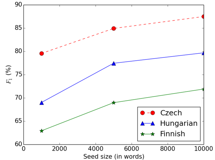
Figure 3: Micro-average $F_{1}$ score on test lexicon while using varying seed sizes for cs, hu and fi.

Size of seed lexicon.

We first test how the size of the seed lexicon affects performance of attribute prediction on the test set. We use the manually constructed lexicons described in §4.2 for experiments. For each language, instead of using the full seed lexicon of 10000 words, we construct subsets of this lexicon by taking 1000 and 5000 randomly sampled words. We then train models obtained in §4.1 on these lexicons and plot the performance on the test set in Figure 3. On average across three languages, we observe that the absolute performance improvement from 1000 to 5000 seed words is $\approx$10% whereas it reduces to $\approx$2% from 5000 to 10000 words.

VForm:Ger		Num:Plur
Clus:105	+	Clus:19	+
Clus:77	+	Clus:97	+
Clus:44	+	Clus:177	+
suffix:ing:{null}	-	suffix:ies:y	-
suffix:ping:{null}	-	suffix:gs:g	-
suffix:ing:er	-	suffix:ons:on	-

Table 10: Highest (upper half) and lowest (lower half) weighted features (with their sign) for predicting a given attribute of English words.

Feature analysis.

Table 10 shows the highest and the lowest weighted features for predicting a given attribute of English words. The highest weighted features for both VForm:Ger and Num:Plur are word clusters, indicating that word clusters exhibit strong syntactic and semantic coherence. More interestingly, it can be seen that for predicting VForm:Ger i.e, continuous verb forms, the lowest weighted features are those morphological transformations that substitute “ing” with something else. Thus, if there exists an edge between the words studying and study, containing the feature: suffix:ing:{null}, the model would correctly predict that studying is VForm:Ger as study is not so and the negative feature weight can flip the label values. The same observation holds true for Num:Plur.

	cs	hu	fi
S + C + MT	87.5	79.9	71.6
S + C	86.5	78.8	68.2
S + MT	85.7	77.0	68.7
C + MT	75.7	57.4	62.2
S + C + MT + P	86.7	66.0	61.3

Table 11: Feature ablation study for induced lexicons evaluated on manually curated gold lexicons. Reported scores are micro-averaged $F_{1}$ score (%) for prediction of lexical attributes. S = suffix; P = prefix; C = clusters; and MT = morphological transformations.

Feature ablation.

One key question is which of the features in our graph are important for projecting morphological attribute-values. Table 3 suggests that this is language specific, which is intuitive, as morphology can be represented more or less regularly through the surface form depending on the language. To understand this, we did a feature ablation study for the three languages with manually curated lexicons (§4.2) using the same feature set as before: clusters, suffix and morphological transformations with paradigm projection. We then leave out each feature to measure how performance drops. Unlike §4.2, we do not average over 10 runs but use a single static graph where features (edges) are added or removed as necessary.

Table 11 contains the results. Critically, all features are required for top accuracy across all languages and leaving out suffix features has the most detrimental effect. This is not surprising considering all three language primarily express morphological properties via suffixes. Furthermore, suffix features help to connect the graph and assist label propagation. Note that the importance of suffix features here is in contrast to the evaluation on treebank derived lexicons in §4.1, where suffix features were only selected for 4 out of 11 languages based on the development data (Table 3), and not for Hungarian and Finnish. This could be due to the nature of the lexicons derived from treebanks versus complete lexicons constructed by humans.

Additionally, we also added back prefix features and found that for all languages, this resulted in a drop in accuracy, particularly for Finnish and Hungarian. The primary reason for this is that prefix features often create spurious edges in the graph. This in and of itself is not a problem for our model, as the edge weights should learn to discount this feature. However, the fact that we sample edges to make inference tractable means that more informative edges could be dropped in favor of those that are only connected via a prefix features.

Prediction examples.

Table 9 shows examples of predictions made by our model for English and Italian. For each language, we first select a random word from the seed lexicon, then we pick one syntactic and one semantically related word to the selected word from the set of unlabeled words. For e.g., in Italian tavola means table, whereas tavoli is the plural form and divano means sofa. We correctly identify attributes for these words.

7 Related Work

We now review the areas of related work.

Lexicon generation.

?) construct morpho-syntactic lexicons by incrementally merging inflectional classes with shared morphological features. Natural language lexicons have often been created from smaller seed lexcions using various methods. ?) use patterns extracted over a large corpus to learn semantic lexicons from smaller seed lexicons using bootstrapping. ?) use distributional similarity scores across instances to propagate attributes using random walks over a graph. ?) learn potential semantic frames for unknown predicates by expanding a seed frame lexicon. Sentiment lexicons containing semantic polarity labels for words and phrases have been created using bootstrapping and graph-based learning [Banea et al., 2008, Mohammad et al., 2009, Velikovich et al., 2010, Takamura et al., 2007, Lu et al., 2011].

Graph-based learning.

In general, graph-based semi-supervised learning is heavily used in NLP [Talukdar and Cohen, 2013, Subramanya and Talukdar, 2014]. Graph-based learning has been used for class-instance acquisition [Talukdar and Pereira, 2010], text classification [Subramanya and Bilmes, 2008], summarization [Erkan and Radev, 2004], structured prediction problems [Subramanya et al., 2010, Das and Petrov, 2011, Garrette et al., 2013] etc. Our work differs from most of these approaches in that we specifically learn how different features shared between the nodes can correspond to either the propagation of an attribute or an inversion of the attribute value (cf. equ 1). In terms of the capability of inverting an attribute value, our method is close to ?), who present a framework to include dissimilarity between nodes and ?), who learn which edges can be excluded for label propagation. In terms of featurizing the edges, our work resembles previous work which measured similarity between nodes in terms of similarity between the feature types that they share [Muthukrishnan et al., 2011, Saluja and Navrátil, 2013]. Our work is also related to graph-based metric learning, where the objective is to learn a suitable distance metric between the nodes of a graph for solving a given problem [Weinberger et al., 2005, Dhillon et al., 2012].

Morphology.

High morphological complexity exacerbates the problem of feature sparsity in many NLP applications and leads to poor estimation of model parameters, emphasizing the need of morphological analysis. Morphological analysis encompasses fields like morphological segmentation [Creutz and Lagus, 2007, Demberg, 2007, Snyder and Barzilay, 2008, Poon et al., 2009, Narasimhan et al., 2015], and inflection generation [Yarowsky and Wicentowski, 2000, Wicentowski, 2004]. Such models of segmentation and inflection generation are used to better understand the meaning and relations between words. Our task is complementary to the task of morphological paradigm generation. Paradigm generation requires generating all possible morphological forms of a given base-form according to different linguistic transformations [Dreyer and Eisner, 2011, Durrett and DeNero, 2013, Ahlberg et al., 2014, Ahlberg et al., 2015, Nicolai et al., 2015, Faruqui et al., 2016], whereas our task requires identifying linguistic transformations between two different word forms.

Low-resourced languages.

Our algorithm can be used to generate morpho-syntactic lexicons for low-resourced languages, where the seed lexicon can be constructed, for example, using crowdsourcing [Callison-Burch and Dredze, 2010, Irvine and Klementiev, 2010]. Morpho-syntactic resources have been developed for east-european languages like Slovene [Dzeroski et al., 2000, Erjavec, 2004], Bulgarian [Simov et al., 2004] and highly agglutinative languages like Turkish [Sak et al., 2008]. Morpho-syntactic lexicons are crucial components in acousting modeling and automatic speech recognition, where they have been developed for low-resourced languages [Huet et al., 2008, Besacier et al., 2014].

One alternative method to extract morphosyntactic lexicons is via parallel data [Das and Petrov, 2011]. However, such methods assume that both the source and target langauges are isomorphic with respect to morphology. This can be the case with attributes like coarse part-of-speech or case, but is rarely true for other attributes like gender, which is very language specific.

8 Future Work

There are three major ways in which the current model can be possibly improved.

Joint learning and propagation.

In the current model, we are first learning the weights in a supervised manner (§3.1) and then propagating labels across nodes in a semi-supervised step with fixed feature weights (§3.2). These can also be performed jointly: perform one iteration of weight learning, propagate labels using these weights, perform another iteration of weight learning assuming empirical labels as gold labels and continue to learn and propagate until convergence. This joint learning would be slower than the current approach as propagating labels across the graph is an expensive step.

Multi-label classifcation.

We are currently using the binary relevance method which trains a binary classifier for every attribute independently [Godbole and Sarawagi, 2004, Zhang and Zhou, 2005] with paradigm projection as a post-processing step (§3.3). Thus we are accounting for attribute correlations only at the end. We can instead model such correlations as constraints during the learning step to obtain better solutions [Ghamrawi and McCallum, 2005, Tsoumakas and Katakis, 2006, Fürnkranz et al., 2008, Read et al., 2011].

Richer feature set.

In addition our model can benefit from a richer set of features. Word embeddings can be used to connect word node which are similar in meaning [Mikolov et al., 2013]. We can use existing morphological segmentation tools to discover the morpheme and inflections of a word to connect it to word with similar inflections which might be better than the crude suffix or prefix features. We can also use rich lexical resources like Wiktionary to extract relations between words that can be encoded on our graph edges.

9 Conclusion

We have presented a graph-based semi-supervised method to construct large annotated morpho-syntactic lexicons from small seed lexicons. Our method is language independent and we have constructed lexicons for 11 different languages. We showed that the lexicons thus constructed help improve performance in morphological tagging and dependency parsing, when used as features.

References

- [Agić et al., 2015] Željko Agić, Maria Jesus Aranzabe, Aitziber Atutxa, Cristina Bosco, Jinho Choi, Marie-Catherine de Marneffe, Timothy Dozat, Richárd Farkas, Jennifer Foster, Filip Ginter, Iakes Goenaga, Koldo Gojenola, Yoav Goldberg, Jan Hajič, Anders Trærup Johannsen, Jenna Kanerva, Juha Kuokkala, Veronika Laippala, Alessandro Lenci, Krister Lindén, Nikola Ljubešić, Teresa Lynn, Christopher Manning, Héctor Alonso Martínez, Ryan McDonald, Anna Missilä, Simonetta Montemagni, Joakim Nivre, Hanna Nurmi, Petya Osenova, Slav Petrov, Jussi Piitulainen, Barbara Plank, Prokopis Prokopidis, Sampo Pyysalo, Wolfgang Seeker, Mojgan Seraji, Natalia Silveira, Maria Simi, Kiril Simov, Aaron Smith, Reut Tsarfaty, Veronika Vincze, and Daniel Zeman. 2015. Universal dependencies 1.1. LINDAT/CLARIN digital library at Institute of Formal and Applied Linguistics, Charles University in Prague.
- [Ahlberg et al., 2014] Malin Ahlberg, Markus Forsberg, and Mans Hulden. 2014. Semi-supervised learning of morphological paradigms and lexicons. In Proc. of EACL.
- [Ahlberg et al., 2015] Malin Ahlberg, Markus Forsberg, and Mans Hulden. 2015. Paradigm classification in supervised learning of morphology. In Proc. of NAACL.
- [Alfonseca et al., 2010] Enrique Alfonseca, Marius Pasca, and Enrique Robledo-Arnuncio. 2010. Acquisition of instance attributes via labeled and related instances. In Proc. of SIGIR.
- [Arisoy et al., 2010] Ebru Arisoy, Murat Saraçlar, Brian Roark, and Izhak Shafran. 2010. Syntactic and sub-lexical features for Turkish discriminative language models. In Proc. of ICASSP.
- [Banea et al., 2008] Carmen Banea, Janyce M. Wiebe, and Rada Mihalcea. 2008. A bootstrapping method for building subjectivity lexicons for languages with scarce resources. In Proc. of LREC.
- [Bengio et al., 2006] Yoshua Bengio, Olivier Delalleau, and Nicolas Le Roux. 2006. Label propagation and quadratic criterion. In Semi-Supervised Learning. MIT Press.
- [Besacier et al., 2014] Laurent Besacier, Etienne Barnard, Alexey Karpov, and Tanja Schultz. 2014. Automatic speech recognition for under-resourced languages: A survey. Speech Communication, 56:85–100.
- [Bohnet and Nivre, 2012] Bernd Bohnet and Joakim Nivre. 2012. A transition-based system for joint part-of-speech tagging and labeled non-projective dependency parsing. In Proc. of EMNLP.
- [Callison-Burch and Dredze, 2010] Chris Callison-Burch and Mark Dredze. 2010. Creating speech and language data with amazon’s mechanical turk. In Proc. of NAACL Workshop on Creating Speech and Language Data with Amazon’s Mechanical Turk.
- [Clark, 2003] Alexander Clark. 2003. Combining distributional and morphological information for part of speech induction. In Proc. of EACL.
- [Creutz and Lagus, 2007] Mathias Creutz and Krista Lagus. 2007. Unsupervised models for morpheme segmentation and morphology learning. ACM Transactions on Speech and Language Processing (TSLP), 4(1):3.
- [Das and Petrov, 2011] Dipanjan Das and Slav Petrov. 2011. Unsupervised part-of-speech tagging with bilingual graph-based projections. In Proc. of ACL.
- [Das and Smith, 2012] Dipanjan Das and Noah A. Smith. 2012. Graph-based lexicon expansion with sparsity-inducing penalties. In Proc. of NAACL.
- [De Marneffe et al., 2014] Marie-Catherine De Marneffe, Timothy Dozat, Natalia Silveira, Katri Haverinen, Filip Ginter, Joakim Nivre, and Christopher D. Manning. 2014. Universal stanford dependencies: A cross-linguistic typology. In Proceedings of LREC.
- [Demberg, 2007] Vera Demberg. 2007. A language-independent unsupervised model for morphological segmentation. In Proc. of ACL.
- [Denis and Sagot, 2009] Pascal Denis and Benoît Sagot. 2009. Coupling an annotated corpus and a morphosyntactic lexicon for state-of-the-art POS tagging with less human effort. In Proc. of PACLIC.
- [Dhillon et al., 2012] Paramveer S. Dhillon, Partha Talukdar, and Koby Crammer. 2012. Metric learning for graph-based domain adaptation. In Proc. of COLING.
- [Dreyer and Eisner, 2011] Markus Dreyer and Jason Eisner. 2011. Discovering morphological paradigms from plain text using a Dirichlet process mixture model. In Proc. of EMNLP.
- [Dryer, 2013] Matthew S. Dryer. 2013. Prefixing vs. Suffixing in Inflectional Morphology. Max Planck Institute for Evolutionary Anthropology.
- [Duchi et al., 2011] John Duchi, Elad Hazan, and Yoram Singer. 2011. Adaptive subgradient methods for online learning and stochastic optimization. The Journal of Machine Learning Research, 12:2121–2159.
- [Dukes and Habash, 2010] Kais Dukes and Nizar Habash. 2010. Morphological annotation of quranic Arabic. In Proc. of LREC.
- [Durrett and DeNero, 2013] Greg Durrett and John DeNero. 2013. Supervised learning of complete morphological paradigms. In Proc. of NAACL.
- [Dzeroski et al., 2000] Saso Dzeroski, Tomaz Erjavec, and Jakub Zavrel. 2000. Morphosyntactic tagging of Slovene: Evaluating taggers and tagsets. In Proc. of LREC.
- [Erjavec, 2004] Tomaz Erjavec. 2004. Multext-east version 3: Multilingual morphosyntactic specifications, lexicons and corpora. In Proc. of LREC.
- [Erkan and Radev, 2004] Günes Erkan and Dragomir R. Radev. 2004. Lexrank: Graph-based lexical centrality as salience in text summarization. Journal of Artificial Intelligence Research, 22(1):457–479.
- [Eskander et al., 2013] Ramy Eskander, Nizar Habash, and Owen Rambow. 2013. Automatic extraction of morphological lexicons from morphologically annotated corpora. In Proc. of EMNLP.
- [Faruqui and Padó, 2010] Manaal Faruqui and Sebastian Padó. 2010. Training and evaluating a German named entity recognizer with semantic generalization. In Proc. of KONVENS.
- [Faruqui et al., 2016] Manaal Faruqui, Yulia Tsvetkov, Graham Neubig, and Chris Dyer. 2016. Morphological inflection generation using character sequence to sequence learning. arXiv:1104.2086.
- [Ferng and Lin, 2011] Chun-Sung Ferng and Hsuan-Tien Lin. 2011. Multi-label classification with error-correcting codes. In Proc. of ACML.
- [Fürnkranz et al., 2008] Johannes Fürnkranz, Eyke Hüllermeier, Eneldo Loza Mencía, and Klaus Brinker. 2008. Multilabel classification via calibrated label ranking. Machine learning, 73(2):133–153.
- [Garrette et al., 2013] Dan Garrette, Jason Mielens, and Jason Baldridge. 2013. Real-world semi-supervised learning of POS-taggers for low-resource languages. In Proc. of ACL.
- [Ghamrawi and McCallum, 2005] Nadia Ghamrawi and Andrew McCallum. 2005. Collective multi-label classification. In Proc. of CIKM.
- [Giménez and Marquez, 2004] Jesús Giménez and Lluís Marquez. 2004. Svmtool: A general POS tagger generator based on support vector machines. In Proc. of LREC.
- [Godbole and Sarawagi, 2004] Shantanu Godbole and Sunita Sarawagi. 2004. Discriminative methods for multi-labeled classification. In Proc. of KDD.
- [Goldberg et al., 2007] Andrew B. Goldberg, Xiaojin Zhu, and Stephen J. Wright. 2007. Dissimilarity in graph-based semi-supervised classification. In Proc. of AISTATS.
- [Goldberg et al., 2009] Yoav Goldberg, Reut Tsarfaty, Meni Adler, and Michael Elhadad. 2009. Enhancing unlexicalized parsing performance using a wide coverage lexicon, fuzzy tag-set mapping, and EM-HMM-based lexical probabilities. In Proc. of EACL.
- [Green and DeNero, 2012] Spence Green and John DeNero. 2012. A class-based agreement model for generating accurately inflected translations. In Proc. of ACL.
- [Hajič and Hladká, 1998] Jan Hajič and Barbora Hladká. 1998. Tagging inflective languages: Prediction of morphological categories for a rich, structured tagset. In Proc. of COLING.
- [Hajič, 2000] Jan Hajič. 2000. Morphological tagging: Data vs. dictionaries. In Proc. of NAACL.
- [Hsu et al., 2009] Daniel Hsu, Sham Kakade, John Langford, and Tong Zhang. 2009. Multi-label prediction via compressed sensing. In Proc. of NIPS.
- [Huet et al., 2008] Stéphane Huet, Guillaume Gravier, and Pascale Sébillot. 2008. Morphosyntactic resources for automatic speech recognition. In Proc. of LREC.
- [Irvine and Klementiev, 2010] Ann Irvine and Alexandre Klementiev. 2010. Using mechanical turk to annotate lexicons for less commonly used languages. In Proc. of NAACL Workshop on Creating Speech and Language Data with Amazon’s Mechanical Turk.
- [Ising, 1925] Ernst Ising. 1925. Beitrag zur theorie des ferromagnetismus. Zeitschrift für Physik A Hadrons and Nuclei, 31(1):253–258.
- [Kneser and Ney, 1993] Reinhard Kneser and Hermann Ney. 1993. Improved clustering techniques for class-based statistical language modelling. In Proc. of Eurospeech.
- [Kokkinakis et al., 2000] Dimitrios Kokkinakis, Maria Toporowska-Gronostaj, and Karin Warmenius. 2000. Annotating, disambiguating & automatically extending the coverage of the Swedish SIMPLE lexicon. In Proc. of LREC.
- [Koo et al., 2008] Terry Koo, Xavier Carreras, and Michael Collins. 2008. Simple semi-supervised dependency parsing. In Proc. of ACL.
- [Kübler et al., 2009] Sandra Kübler, Ryan McDonald, and Joakim Nivre. 2009. Dependency parsing. Synthesis Lectures on Human Language Technologies. Morgan & Claypool Publishers.
- [Lu et al., 2011] Yue Lu, Malu Castellanos, Umeshwar Dayal, and ChengXiang Zhai. 2011. Automatic construction of a context-aware sentiment lexicon: An optimization approach. In Proc. of WWW.
- [Martin et al., 1998] Sven Martin, Jörg Liermann, and Hermann Ney. 1998. Algorithms for bigram and trigram word clustering. Speech communication, 24(1):19–37.
- [McDonald et al., 2013] Ryan McDonald, Joakim Nivre, Yvonne Quirmbach-Brundage, Yoav Goldberg, Dipanjan Das, Kuzman Ganchev, Keith B. Hall, Slav Petrov, Hao Zhang, Oscar Täckström, Claudia Bedini, Núria B. Castelló, and Jungmee Lee. 2013. Universal dependency annotation for multilingual parsing. In Proc. of ACL.
- [Mikolov et al., 2013] Tomas Mikolov, Wen-tau Yih, and Geoffrey Zweig. 2013. Linguistic regularities in continuous space word representations. In Proc. of NAACL.
- [Minkov et al., 2007] Einat Minkov, Kristina Toutanova, and Hisami Suzuki. 2007. Generating complex morphology for machine translation. In Proc. of ACL.
- [Mohammad et al., 2009] Saif Mohammad, Cody Dunne, and Bonnie Dorr. 2009. Generating high-coverage semantic orientation lexicons from overtly marked words and a thesaurus. In Proc. of EMNLP.
- [Moore, 2015] Robert Moore. 2015. An improved tag dictionary for faster part-of-speech tagging. In Proc. of EMNLP.
- [Müller and Schuetze, 2015] Thomas Müller and Hinrich Schuetze. 2015. Robust morphological tagging with word representations. In Proceedings of NAACL.
- [Müller et al., 2013] Thomas Müller, Helmut Schmid, and Hinrich Schütze. 2013. Efficient higher-order CRFs for morphological tagging. In Proc. of EMNLP.
- [Muthukrishnan et al., 2011] Pradeep Muthukrishnan, Dragomir Radev, and Qiaozhu Mei. 2011. Simultaneous similarity learning and feature-weight learning for document clustering. In Proc. of TextGraphs.
- [Narasimhan et al., 2015] Karthik Narasimhan, Regina Barzilay, and Tommi Jaakkola. 2015. An unsupervised method for uncovering morphological chains. Transactions of the Association for Computational Linguistics, 3:157–167.
- [Nicolai et al., 2015] Garrett Nicolai, Colin Cherry, and Grzegorz Kondrak. 2015. Inflection generation as discriminative string transduction. In Proc. of NAACL.
- [Nießen and Ney, 2004] Sonja Nießen and Hermann Ney. 2004. Statistical machine translation with scarce resources using morpho-syntactic information. Computational Linguistics, 30(2).
- [Oflazer and Kuruöz, 1994] Kemal Oflazer and Ìlker Kuruöz. 1994. Tagging and morphological disambiguation of Turkish text. In Proc. of ANLP.
- [Owoputi et al., 2013] Olutobi Owoputi, Brendan O’Connor, Chris Dyer, Kevin Gimpel, Nathan Schneider, and Noah A. Smith. 2013. Improved part-of-speech tagging for online conversational text with word clusters. In Proc. of NAACL.
- [Pirinen, 2011] Tommi A Pirinen. 2011. Modularisation of finnish finite-state language description—towards wide collaboration in open source development of a morphological analyser. In Proc. of NODALIDA.
- [Poon et al., 2009] Hoifung Poon, Colin Cherry, and Kristina Toutanova. 2009. Unsupervised morphological segmentation with log-linear models. In Proc. of NAACL.
- [Ratnaparkhi, 1996] Adwait Ratnaparkhi. 1996. A maximum entropy model for part-of-speech tagging. In Proc. of EMNLP.
- [Read et al., 2011] Jesse Read, Bernhard Pfahringer, Geoff Holmes, and Eibe Frank. 2011. Classifier chains for multi-label classification. Machine Learning, 85(3):333–359.
- [Sak et al., 2008] Haşim Sak, Tunga Güngör, and Murat Saraçlar. 2008. Turkish language resources: Morphological parser, morphological disambiguator and web corpus. In Proc. of ANLP.
- [Saluja and Navrátil, 2013] Avneesh Saluja and Jirı Navrátil. 2013. Graph-based unsupervised learning of word similarities using heterogeneous feature types. In Proc. of TextGraphs.
- [Schmid, 1994] Helmut Schmid. 1994. Probabilistic part-of-speech tagging using decision trees. In Proc. of the International Conference on New Methods in Language Processing.
- [Simov et al., 2004] Kiril Ivanov Simov, Petya Osenova, Sia Kolkovska, Elisaveta Balabanova, and Dimitar Doikoff. 2004. A language resources infrastructure for Bulgarian. In Proc. of LREC.
- [Smith et al., 2005] Noah A. Smith, David A. Smith, and Roy W. Tromble. 2005. Context-based morphological disambiguation with random fields. In Proc. of EMNLP.
- [Snyder and Barzilay, 2008] Benjamin Snyder and Regina Barzilay. 2008. Unsupervised multilingual learning for morphological segmentation. In Proc. of ACL.
- [Soricut and Och, 2015] Radu Soricut and Franz Och. 2015. Unsupervised morphology induction using word embeddings. In Proc. of NAACL.
- [Subramanya and Bilmes, 2008] Amarnag Subramanya and Jeff Bilmes. 2008. Soft-supervised learning for text classification. In Proc. of EMNLP.
- [Subramanya and Talukdar, 2014] Amarnag Subramanya and Partha Pratim Talukdar. 2014. Graph-based semi-supervised learning. Synthesis Lectures on Artificial Intelligence and Machine Learning, 8(4).
- [Subramanya et al., 2010] Amarnag Subramanya, Slav Petrov, and Fernando Pereira. 2010. Efficient graph-based semi-supervised learning of structured tagging models. In Proc. of EMNLP.
- [Täckström et al., 2012] Oscar Täckström, Ryan McDonald, and Jakob Uszkoreit. 2012. Cross-lingual word clusters for direct transfer of linguistic structure. In Proc. of NAACL.
- [Takamura et al., 2007] Hiroya Takamura, Takashi Inui, and Manabu Okumura. 2007. Extracting semantic orientations of phrases from dictionary. In Proc. of NAACL.
- [Talukdar and Cohen, 2013] Partha Pratim Talukdar and William Cohen. 2013. Scaling graph-based semi-supervised learning to large number of labels using count-min sketch. In Proc. of AISTATS.
- [Talukdar and Pereira, 2010] Partha Pratim Talukdar and Fernando Pereira. 2010. Experiments in graph-based semi-supervised learning methods for class-instance acquisition. In Proc. of ACL.
- [Talukdar et al., 2012] Partha Pratim Talukdar, Derry Wijaya, and Tom Mitchell. 2012. Acquiring temporal constraints between relations. In Proc. of CIKM.
- [Thelen and Riloff, 2002] Michael Thelen and Ellen Riloff. 2002. A bootstrapping method for learning semantic lexicons using extraction pattern contexts. In Proc. of ACL.
- [Trón et al., 2006] Viktor Trón, Péter Halácsy, Péter Rebrus, András Rung, Péter Vajda, and Eszter Simon. 2006. Morphdb.hu: Hungarian lexical database and morphological grammar. In Proc. of LREC.
- [Tsoumakas and Katakis, 2006] Grigorios Tsoumakas and Ioannis Katakis. 2006. Multi-label classification: An overview. Dept. of Informatics, Aristotle University of Thessaloniki, Greece.
- [Turian et al., 2010] Joseph Turian, Lev Ratinov, and Yoshua Bengio. 2010. Word representations: a simple and general method for semi-supervised learning. In Proc. of ACL.
- [Uszkoreit and Brants, 2008] Jakob Uszkoreit and Thorsten Brants. 2008. Distributed word clustering for large scale class-based language modeling in machine translation. In Proc. of ACL.
- [Velikovich et al., 2010] Leonid Velikovich, Sasha Blair-Goldensohn, Kerry Hannan, and Ryan McDonald. 2010. The viability of web-derived polarity lexicons. In Proc. of NAACL.
- [Wang et al., 2007] Fei Wang, Shijun Wang, Changshui Zhang, and Ole Winther. 2007. Semi-supervised mean fields. In Proc. of AISTATS.
- [Weinberger et al., 2005] Kilian Q. Weinberger, John Blitzer, and Lawrence K. Saul. 2005. Distance metric learning for large margin nearest neighbor classification. In Proc. of NIPS.
- [Wicentowski, 2004] Richard Wicentowski. 2004. Multilingual noise-robust supervised morphological analysis using the wordframe model. In Proc. of SIGPHON.
- [Yarowsky and Wicentowski, 2000] David Yarowsky and Richard Wicentowski. 2000. Minimally supervised morphological analysis by multimodal alignment. In Proc. of ACL.
- [Zhang and Nivre, 2011] Yue Zhang and Joakim Nivre. 2011. Transition-based dependency parsing with rich non-local features. In Proc. of ACL.
- [Zhang and Schneider, 2011] Yi Zhang and Jeff G. Schneider. 2011. Multi-label output codes using canonical correlation analysis. In Proc. of AISTATS.
- [Zhang and Zhou, 2005] Min-Ling Zhang and Zhi-Hua Zhou. 2005. A k-nearest neighbor based algorithm for multi-label classification. In Proc. of IEEE Conference on Granular Computing.
- [Zhu, 2005] Xiaojin Zhu. 2005. Semi-supervised Learning with Graphs. Ph.D. thesis, Carnegie Mellon University, Pittsburgh, PA, USA. AAI3179046.