High S/N Keck and Gemini AO imaging of Uranus during 2012-2014: new cloud patterns, increasing activity, and improved wind measurements.

Abstract

We imaged Uranus in the near infrared from 2012 into 2014, using the Keck/NIRC2 camera and Gemini/NIRI camera, both with adaptive optics. We obtained exceptional signal to noise ratios by averaging 8-16 individual exposures in a planet-fixed coordinate system. These noise-reduced images revealed many low-contrast discrete features and large scale cloud patterns not seen before, including scalloped waveforms just south of the equator, and an associated transverse ribbon wave near 6^∘S. In all three years numerous small (600-700 km wide) and mainly bright discrete features were seen within the north polar region (north of about 55^∘N). Two small dark spots with bright companions were seen at middle latitudes. Over 850 wind measurements were made, the vast majority of which were in the northern hemisphere. Winds at high latitudes were measured with great precision, revealing an extended region of solid body rotation between 62^∘N and at least 83^∘N, at a rate of 4.08$\pm 0.015$^∘/h westward relative to the planet’s interior (radio) rotation of 20.88^∘/h westward. Near-equatorial speeds measured with high accuracy give different results for waves and small discrete features, with eastward drift rates of 0.4^∘/h and 0.1^∘/h respectively. The region of polar solid body rotation is a close match to the region of small-scale polar cloud features, suggesting a dynamical relationship. The winds from prior years and those from 2012-2014 are consistent with a mainly symmetric wind profile up to middle latitudes, with a small asymmetric component of $\sim$0.09^∘/h peaking near $\pm$30^∘, and about 60% greater amplitude if only prior years are included, suggesting a declining mid-latitude asymmetry. While winds at high southern latitudes (50^∘S - 90^∘S) are unconstrained by groundbased observations, a recent reanalysis of 1986 Voyager 2 observations by Karkoschka (2015, Icarus 250, 294-307) has revealed an extremely large north-south asymmetry in this region, which might be seasonal. Greatly increased activity was seen in 2014, including the brightest ever feature seen in K^′ images (de Pater et al. 2015, Icarus 252, 121-128), as well as other significant features, some of which had long lives. Over the 2012-2014 period we identified six persistent discrete features. Three were tracked for more than two years, two more for more than one year, and one for at least 5 months and continuing. Several drifted in latitude towards the equator, and others appeared to exhibit latitudinal oscillations with long periods. We found two pairs of long-lived features that survived multiple passages within their own diameters of each other. Zonally averaged cloud patterns were found to persist over 2012-2014. When averaged over longitude, there is a brightness variation with latitude from 55^∘N to the pole that is similar to effective methane mixing ratio variations with latitude derived from 2012 STIS observations (Sromovsky et al. 2014, Icarus 238, 137-155).

1. Introduction

Visual observers reported detection of zonal bands and occasional spots on Uranus as early as 1870 (Alexander 1965), but a reliable measure of atmospheric motions on Uranus had to wait until 1986, when close-up Voyager-2 images revealed eight discrete cloud features between planetocentric latitudes of 35^∘ S and 70^∘ S (Smith et al. 1986). Tracking these features, combined with one radio occultation wind measurement at 5^∘ S, yielded a crude zonal wind profile (Allison et al. 1991), the main feature of which appeared to be a high-speed ($\sim$250 m/s) prograde jet near 60^∘ S and a weaker broad retrograde equatorial jet. Voyager did not provide wind information in the northern hemisphere, which was near its winter solstice and dark at the time of the encounter. Eleven years later, Hubble Space Telescope (HST) near-IR images of Uranus revealed many more discrete cloud features, enabling the extension of wind measurements into the northern hemisphere (Karkoschka 1998), confirming an approximate N-S symmetry in the wind profile. Groundbased observations from the Keck II telescope, which combined a large aperture, near-IR wavelengths, and adaptive optics, produced a bounty of cloud features far beyond the Hubble results (Hammel et al. 2001, 2005; Sromovsky and Fry 2005; Sromovsky et al. 2007; Hammel et al. 2009; Sromovsky et al. 2009).

The wind profile of Uranus was last updated by Sromovsky et al. (2012c), combining wind observations from the above references with new measurements in 2009-2011 from Gemini, Keck, and HST observatories. Here we use as a reference their 13-term asymmetric Legendre fit given in their Table 6 and plotted in their Fig. 11. This will be hereafter referred to as Model S13A. The main results enabled by their new measurements were: (1) clear definition of the magnitude and latitude of the northern jet peak; (2) discovery that motions north of the peak were consistent with solid body rotation; (3) discovery of a new class of cloud features in the polar regions that resemble cumulus cloud fields and bear similarities to the cloud structure in the polar regions of Saturn; and (4) characterization of the large morphological asymmetry between southern summer polar latitudes and northern spring polar latitudes. The updated profile still suffered from a lack of targets in low latitudes (20^∘ S - 20^∘ N) and in the south polar region, where, save for one UV feature identified by Voyager, no discrete clouds had ever been seen.

The Sromovsky et al. (2012c) work was advanced by the use of high S/N techniques to improve detectability and facilitate tracking of low contrast cloud features. The basic idea was to use long exposures to grow the signal linearly in exposure time while random noise grew as the square root, thus increasing S/N as the square root of the exposure time. To avoid the smearing of long exposures by planetary rotation, we took multiple short exposures, rotated the planet images to the same central meridian longitude, then averaged the de-rotated images. Fry et al. (2012a) verified this process using Keck imagery and applied it to specially designed HST imaging to provide new wind measurements. Sromovsky et al. (2012c) applied it to Gemini imaging in 2011, and to a limited degree to Keck imaging in 2011, though highly variable seeing limited the benefits that were possible. Much improved results were obtained from subsequent observations with better seeing that resulted in better AO performance. The 2012 results shown in Fig. 1, first presented by Sromovsky et al. (2012b) and Fry et al. (2012b), were the most detailed images of Uranus ever obtained up to that time. Features revealed by those images are discussed in Section 5.

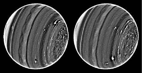
Figure 1.— Keck II de-rotated, averaged, and high-pass filtered H-filter images of Uranus from 25 July (L) and 26 July(R), 2012. The north pole is at the right (about 100^∘ clockwise from up), and the dark band just right of the middle of each image is at $\approx$8.5^∘N (planetographic), the scalloped waveform centered near 4.5^∘S, and the ribbon wave near 6^∘S. Note the narrow bright latitude bands spaced about 2.5^∘ apart in the 48^∘-53^∘range, and the numerous small bright spots north of 55^∘N. The bright narrow feature in the southern hemisphere is the epsilon ring of Uranus.

Since 2007, our view of the north polar region of Uranus improved significantly: at opposition, the the sub-solar latitude reached 19.5^∘N in 2012, 23.5^∘N in 2013, and 27.6^∘N in 2014. This resulted in observations well suited to further refinement of the zonal wind profile in the northern hemisphere and better characterization of its polar cloud features. It also helped to fill in poorly sampled regions, mainly at low latitudes. Fortunate periods of high quality seeing also allowed us to apply high S/N techniques more extensively and thereby detect and track more subtle features. In the following we describe the new observations, the measurement results from each data set, new views of the north polar region of Uranus and the different styles of discrete cloud features located there, new features discovered at low latitudes, and finally, approximate altitude constraints on the cloud features.

2. Observations, image processing, and navigation

Table 1 summarizes Keck and Gemini imaging observations of Uranus acquired from 2012 through 2014. The camera characteristics for each groundbased observing configuration are given in Table 2, in which the pixel scale of 0.02138$\pm$0.0005 arcsec/pixel listed for the Gemini NIRI camera was derived from measurements of Uranus and its satellites in comparison with HORIZONS ephemeris positions, as described by Sromovsky et al. (2012c). We used the Keck II/NIRC2 pixel scale provided by the Keck observatory web site, which we found to be consistent with measurements of the Uranian ring system. For Gemini AO operation, we used a bright Uranian satellite (usually Ariel) as the wavefront reference, while for Keck II AO operation we were able to use Uranus itself, providing a substantial gain in reference object brightness (VMAG=5.6 vs. VMAG$\approx$14) and thus in image quality for similar seeing conditions. Except for the image S/N enhancement, described in more detail by Fry et al. (2012a), image processing and navigation followed the same procedures described by Sromovsky et al. (2009). To aid in long-term tracking of a long lived feature that was first observed in August 2014 (identified as F in a later section), we also used non-proprietary images from HST Program 13712 (Target of Opportunity Observation of an Episodic Storm on Uranus, PI K. Sayanagi) and HST Program 13937 (Hubble 2020: Outer Planet Atmospheres Legacy (OPAL) Program, PI A. Simon).

Table 1Imaging observations used to track and characterize discrete cloud features.

Date	Time Range	Telescope/Camera/Program	PI	Filters (images)
2012/07/25	09:59-12:29	Keck/NIRC2/2012A-N145N2	LAS	H(93), Hc(24), K′(1)
2012/07/26	10:04-15:29	Keck/NIRC2/2012A-N145N2	LAS	H(88), Hc(32)
2012/08/16	10:31-15:41	Keck/NIRC2/2012B-N125N2	LAS	H(91), Hc(56)
2012/09/28	08:20-12:24	Gemini-N/NIRI/GN-2012B-Q-121	LAS	H(11), Hc(10)
2012/09/30	08:15-12:09	Gemini-N/NIRI/GN-2012B-Q-121	LAS	H(8), Hc(9)
2012/10/04	08:58-12:50	Gemini-N/NIRI/GN-2012B-Q-121	LAS	H(11), Hc(12)
2012/10/09	06:17-10:10	Gemini-N/NIRI/GN-2012B-Q-121	LAS	H(11), Hc(11)
2012/11/04	04:17-09:34	Keck/NIRC2/2012B-U011N2	IDP	H(120), Hc(3), K′(1)
2012/11/05	04:11-09:17	Keck/NIRC2/2012B-U011N2	IDP	H(42), Hc(76), K′(2)
2013/08/15	10:35-14:43	Keck/NIRC2/2013B-U009N2	IDP	H(74), CH4S(10), K′(3)
2013/08/16	10:34-15:24	Keck/NIRC2/2013B-U009N2	IDP	H(84), CH4S(14), K′(10)
2014/08/05	11:34-15:36	Keck/NIRC2/2014B-U037N2	IDP	H(64), K′(5), CH4S(8)
2014/08/06	11:24-13:44	Keck/NIRC2/2014B-U037N2	IDP	H(78),J(1),K′(9),CH4S(10)
2014/08/20	13:38-13:44	Keck/NIRC2/2014B-U014N2	IDP	H(2), K′(2)
2014/10/30	08:57-09:03	Gemini-N/NIRI/GN-2014B-DD-5	LAS	H(4)
2014/11/09	09:19-09:25	Gemini-N/NIRI/GN-2014B-DD-5	LAS	H(4)
2014/11/26	07:14-07:48	Gemini-N/NIRI/GN-2014B-DD-5	LAS	H(4), K′(4), Hc(8)
2015/01/08	07:05-07:24	Gemini-N/NIRI/GN-2014B-DD-5	LAS	H(4), K′(4), Hc(8)

NOTE: Times are UTC. PI codes are LAS for Sromovsky, IDP for de Pater. Filter bands are: H(1.48-1.78 $\mu$m), Hcont(1.57-1.59 $\mu$m), CH4S(1.53-1.66 $\mu$m ), and K^′(1.95-2.3 $\mu$m).

Table 2Telescope/camera characteristics.

	Mirror		Pixel	Diff. limit
Telescope	Diam.	Camera	size	@ wavelength
Gemini-N	8 m	NIRI	0.02138′′	0.05′′ @ 1.6 $\mu$m
Keck II	10 m	NIRC2-NA	0.00994′′	0.04′′ @ 1.6 $\mu$m

NOTES: Both groundbased telescopes have adaptive optics capability, but only Keck II can use Uranus itself as the wave front reference. Our Gemini observations had to use a satellite of Uranus for the wave front reference.

Almost all our observations were designed for high S/N imaging and were successful to varying degrees, mainly dependent on seeing conditions. A sampling of the mosaicked and averaged H-band images from the Keck and Gemini data sets is provided in Fig. 2. Most of these images were averaged in groups of eight 2-minute exposures. The exceptions are for the Gemini images in which all images during the night were averaged together (this required removal of approximate zonal wind displacements as well as planet rotation). In Fig. 2 each image is followed by a version with enhanced small-scale feature contrast, obtained by replacing the original image I by I+30$\times$(I-smooth(I)), using a smoothing length of 0.13^′′ (13 pixels in Keck images). In most cases the Keck AO images provide a level of detail far superior to that obtained from Gemini or HST. In one case, however, a fortuitous natural seeing of 0.37^′′ resulted in an excellent Gemini image (G and H in Fig. 2), providing slightly better S/N though at a slightly lower resolution (see Fig. 2G).

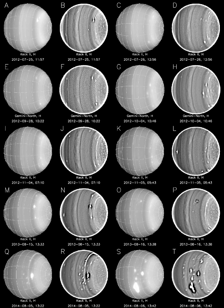
Figure 2.— Sample high-S/N images from the major data sets listed in Table 1. Each image is followed by a high-frequency amplified version, in which the difference between a smoothed version and the original image is added back to the original image after the difference is multiplied by a factor of 30. The box-car smoothing length was 0.13 arcseconds. The grids shown are at intervals of 15^∘ in planetographic latitude and 30^∘ in longitude. Note the increased activity in 2014.

Many of these images reveal a low-latitude waveform just south of the equator, the best examples of which are seen in Fig. 2, panels B (25 July 2012) and J (4 November 2012). The wave is also evident in several other images, including the Gemini image from 4 October 2012. When first observed in 2012, it was suggested that this might be an unstable feature because of morphological similarities to unstable waves in high-shear regions. The persistence of the waveform, and the lack of evidence for high (or any) zonal wind shear in the region of the wave, suggests that other explanations might be needed.

These images also show a persistence of small cloud features at high northern latitudes, although the contrast of these features in the 2014 images seems to be reduced, perhaps by a developing haze in the north polar region (de Pater et al. 2015) (note the brighter near-pole region in 2014 relative to that in 2012). There is a general lack of discrete cloud features south of 30^∘N, with the striking exception of 2014 images (Fig. 2Q-T), which not only display numerous cloud features in this region, but also several unusually bright ones, including the brightest ever seen in K^′ images (de Pater et al. 2015), and the second brightest ever seen in H-band images. The brightest feature in H-band images (Sromovsky et al. 2007) was seen in 2005 at a planetographic latitude of 31^∘N.

We also acquired Hcont images in groups of 12 (for Keck observations). Images with the Hcont filter (not shown) differ from the H-filter images in having relatively brighter mid latitudes, more noise (due to less throughput in the narrow-band filter), generally lower contrast, and fewer visible cloud features. The average penetration depths of light within these filter bands into a clear Uranus atmosphere are shown in Fig. 3. The different vertical weighting of Hcont images allows the combination of H and Hcont images to constrain the vertical location of cloud features. Limited imaging with CH4S and K^′ filters provided additional constraints, which are all discussed in Section 9.2.

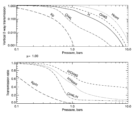
Figure 3.— Vertical 2-way transmission of a clear uranian atmosphere as a function of pressure for filter bands used in groundbased observations (top) and transmission ratios (bottom).

3. Cloud tracking

3.1. Methodology

We used maximum correlation tracking, as described by Sromovsky et al. (2012c), to maximize the number of cloud targets that could be usefully tracked and to reduce errors in position measurements. We displayed an image sequence as a stacked series of narrow horizontal strips, each containing a rectangular projection covering a specified range of longitudes and a narrow range of latitudes, using 0.2^∘$\times$0.2^∘ image pixels, as illustrated in Fig. 4. For each cloud target visible in the selected latitude range, a reference image is selected and a target box is adjusted in size and position in the reference image so that the box contains the cloud feature and a small region outside of it. Target boxes in other images are initially positioned using a prior wind profile; then the guess is manually adjusted as needed to insure that all target boxes contain the target feature. The positions of the target boxes in all but the reference images are then automatically precision-adjusted to maximize the cross correlation between the reference target box signal variations and those contained in each of the other boxes. The correlation coefficient $r$ was computed using

$$r=\frac{\Sigma(x_{i}-\bar{x})(y_{i}-\bar{y})}{\sqrt{\Sigma(x_{i}-\bar{x})^{2}}\sqrt{\Sigma(y_{i}-\bar{y})^{2}}}$$ (1)

where $x_{i}$ and $y_{i}$ are brightness values at the $i$th pixel location in images $X$ and $Y$ respectively, $\bar{x}$ and $\bar{y}$ their average values, and the summation is over all corresponding pixels in the target boxes.

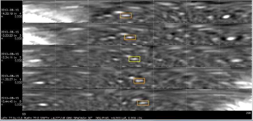
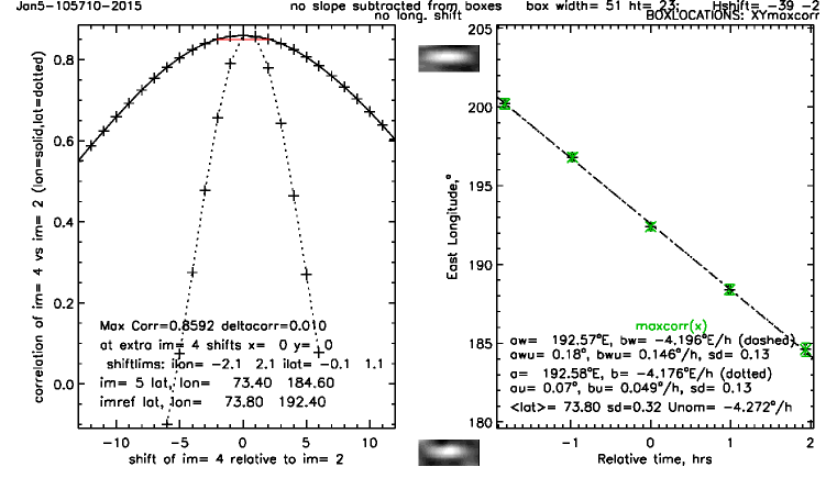
Figure 4.— Illustration of our manually guided correlated tracking method. The top panel displays five rectangular projections centered at 77^∘N, spanning 240^∘ in longitude and 20^∘ in latitude, vertically stacked with the earliest image at the bottom. At this point the box outlines surrounding the selected target feature have been moved to produce the maximum cross correlations with the feature in the reference box at the center of the screen. Box longitudes vs. time are plotted at the bottom right along with best-fit linear drift rate coefficients for the model $\phi(t)=$a + b $(t-t_{0})$) for both unweighted and weighted fits, with coefficients (a,b) and (aw,bw) respectively), with (au, bu) and (awu, bwu) denoting uncertainties. The initial guessed drift rate value (Unom) is also shown in the legend. Sample plots of correlation coefficient versus latitude and longitude displacements of the image-4 sampling box relative to image-2 sampling box are shown in the lower left panel.

To reduce the impact of large-scale variations such as produced by latitude bands, we use high-pass filters to display local contrast and remove large-scale image slopes before correlation. Measurements of longitude and latitude vs. time were fit to straight lines using both unweighted and weighted fits, and assigned errors that were the larger of the two estimates obtained from linear regression. The results are produced in real time as each target is tracked and displayed as illustrated in Fig. 4. Errors in latitude and longitude are estimated in two ways. The first is an a priori computation of the scaled root sum of squared errors produced by displacements of one image pixel in both dimensions. These errors, which provide the basis for the weighted fits, vary appropriately with view angle and position on the disk and are important when the number of samples is small. But, when the number of samples is large, the second and more accurate error estimate is computed from the RMS deviation of the measurements from a straight line fit, as it includes both navigation errors as well as target identification and tracking errors. This second estimate provides the basis for the unweighted fits.

3.2. Cloud tracking statistics for 2012-2014 data sets

We made over 850 measurements of cloud feature drift rates in the 2012-2014 images, mostly tracking small discrete cloud features, with each drift rate based on from 3 to 11 individual position measurements. For comparison, the Voyager mission returned only 8 wind measurements (Smith 1986) and the recent extensive reanalysis of Voyager images by Karkoschka (2015) yielded 27 trackable discrete features. The Keck data from 2014 provided an exceptional number of measurements, which is a result of the increased activity of Uranus in 2014, not due to exceptional image quality. In fact, image quality during the 5-6 August observing run was a little below par for our typical Keck II observations.

The distribution of measurements in longitude and latitude segregated by data set is provided in Fig. 5. As can be seen from this figure and the plot of statistical properties in Fig. 6, the measurements are heavily weighted to the northern hemisphere, where discrete cloud targets are most numerous. Furthermore, because the sub-earth and sub-solar points are in the northern hemisphere, the cloud features there are visible over a longer time span during a given observing night than is possible at southern latitudes. Consequently, even were the distribution of targets uniform, there would still be more measurements and more accurate measurements in the northern hemisphere. Especially numerous were cloud features north of 45^∘ N. Not surprisingly, these data sets provided no observations below about 40^∘ S.

The distribution of wind measurements over a wide range of longitudes for most data sets achieves a major objective of our high S/N observing program, i.e. to avoid having wind results dominated by a few large features and features in their immediate surroundings, which might be generated by the large feature and travel along with it, even at a different latitude. Fig. 5 also classifies each drift rate measurement according to median correlation of the set of position measurements used to determine the drift rate. The darker the plotted point, the higher the median correlation, and the more likely the cloud did not evolve much during the tracked interval, and was elevated above the noise level, improving the accuracy of the position tracking. Most of the measurements obtained median correlation peaks that were between 0.8 and 1 (Fig. 6E). Near-equatorial features that appear to be associated with waves had some of the lowest median correlation peaks (0.4-0.6).

Discrete cloud features were tracked in sequences of up to eleven images, always in at least three, and most in 5-9 image sequences. The standard deviation of latitude measurements for a given cloud target (Fig. 6B) was usually within one or two map pixels (0.2^∘/pixel), as were longitude measurements, which were all determined by correlation. Most features were tracked using target boxes between 3^∘ and 10^∘ in longitude and 2-5^∘ in latitude (Fig. 6E-F). For compact features both latitude and longitude positions of the cloud boxes were determined by correlation, which was done to compensate for small navigation errors between images. But navigation errors are responsible for only part of the dispersion in latitude measurements. The remainder is due to evolution in cloud target morphology over time, and to some degree it may be due to latitudinal drifts and/or oscillations, though it is only tracking over long time intervals that revealed any statistically significant latitudinal motion.

Figure 6 also shows that a subset of our measurements used correlation boxes that were wide (in longitude) and narrow (in latitude), which were designed to group together a number of nearby features at the same latitude to allow a more precise determination of their group drift rate within a single transit. These were usually 1.2^∘ in latitude and 50-100^∘ in longitude. For these boxes we did correlation tracking of only the longitudinal displacement to avoid latitude shifts due to the brightest cloud feature included.

A key factor in the resulting accuracy of the wind measurement was the length of time that a target could be tracked (Fig. 6H). The shortest time that we considered even marginally useful was one hour. Typically the best we could obtain within a single night of observing was a little over 4 hours. When a feature could be identified on successive nights, which was possible mostly only for higher-latitude features, wind accuracy improved dramatically. For some targets tracked in Gemini data sets we were able to track targets over a span of several hundred hours (with significant coverage gaps of course). Even longer tracking times were achieved for six persistent discrete features identified mainly in Keck imagery and discussed in Section 5.2.

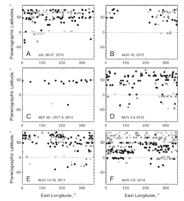
Figure 5.— Spatial distribution of measured drift rates by observing run, except for C in which several runs are include. Filled circles indicate median correlation for the measurement plotted, using black for 0.9 or greater, dark gray for 0.8 to 0.9, and light gray for less than 0.8. The lower correlations seen just south of the equator in all but panel C, are based on wave feature tracking. The limited longitudinal coverage in B is typical of just one night of observing. The large number of measurements in 2014 (F) is due to increased activity of Uranus, not improved image quality, which is actually worse than most of the prior Keck observations. The broad longitude distribution in each data set show that results at most latitudes are not dominated by just a few discrete features. High correlations indicate accurate tracking.

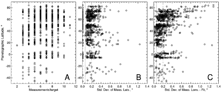
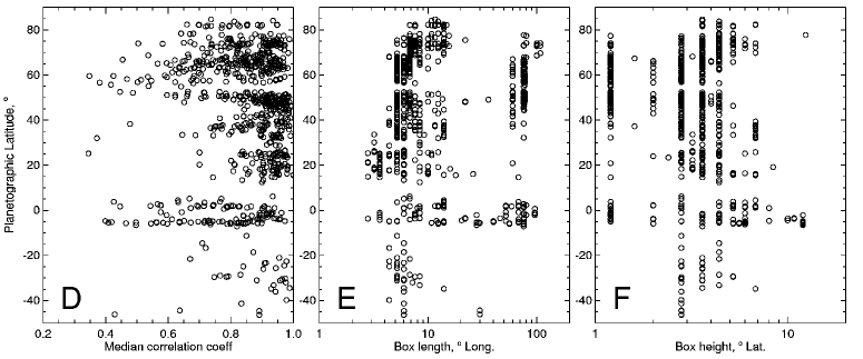
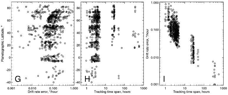
Figure 6.— Statistical properties of cloud tracked wind measurements vs. latitude: measurements per target (A), standard deviation of measured latitudes from mean (B), standard deviation of measured longitudes relative to the linear fit of longitude vs. time (C), median correlation coefficient between reference cloud and other images of the same cloud (D), target box length (E), target box height (F), drift rate error (G), and time over which a cloud target was tracked (H). Also shown is a plot of drift rate error vs. tracking time span (I).

3.3. Wind measurements obtained from 2012-2014 data sets

The measurements of the westward drift rate relative to the planet’s longitude system are plotted in Fig. 7, where the full data set of 852 measurements is shown in panel A and a subset including only the 163 most accurate measurements in panel B. These two samples are both compared to the Model S13A, shown as a solid curve, and its reflection about the equator shown as the dotted curve. Points falling on the solid curve would tend to confirm the asymmetry previously inferred. Points between the solid and dotted curves would be more consistent with hemispheric symmetry. Since many of our points fall between these two curves, they suggest somewhat less asymmetry than the prior fit. A more detailed analysis of asymmetry is discussed in Section 4.3.

The largest discrepancies between our new observations and the prior Legendre polynomial fit are near the equator and at high latitudes (Fig. 7). In the north polar region, we find a very robust determination of solid body rotation between 62^∘N and 83^∘N, with a westward rotation rate of 4.1^∘/h relative to the planet’s interior rotation rate of 360^∘/17.24h (=20.88^∘/h). That corresponds to a rotational period of 14.41 hours. The prior Legendre polynomial fit has a relative solid body rotational period of 4.3^∘/h, which is less accurate because of fewer measurements, shorter time tracks, and poorer views of high latitudes.

The second discrepancy with the prior wind profile occurs within 6^∘ of the equator. Measurements with the highest accuracy, based on small discrete clouds of high contrast in 2014 images, yield a very small longitudinal drift of 0.1^∘/h eastward between 1^∘ N and 5^∘ S, while the Legendre fit suggests a drift rate of about 0.4^∘/h to the east. That latter drift rate is more compatible with our lower accuracy measurements in this region, which are based on much more diffuse low-contrast features that have relatively low median correlations, or on wave patterns, such as the nearly sinusoidal dark ribbon visible in several of the images in Fig. 2. It is clear that the wave features drift eastward at close to four times the rate observed for the small discrete features tracked in 2014. Drift rates similar to those measured for wave features in our 2012-2014 observations were also observed by Hammel et al. (2005), who found, in their 2003 images of Uranus, “fuzzy patches” within 2^∘ of the equator moving with an average eastward velocity of 47 m/s, or 0.38^∘/h eastward. Similar features measured by Sromovsky et al. (2012c) 2-3^∘ north of the equator, were found to move eastward at a rate of 0.51^∘/h. Interestingly, Sromovsky et al. (2012c) found the features to have roughly a 40^∘ spacing in longitude, while Hammel et al. (2005) found a 30^∘ spacing, but with gaps. The features in our 2012-2014 observations seem to be near 36^∘, and not quite twice the period of the ribbon wave. (This is presented in Section 7.) These high S/N images indicate that not all the equatorial features match the average spacing of 36^∘; some have considerably different spacings. There are also gaps and regions where features are spread out and difficult to locate. It is not clear that the wave producing these features extends entirely around the planet. The variability of these features may explain the discrepancies between prior measurements of their spacings.

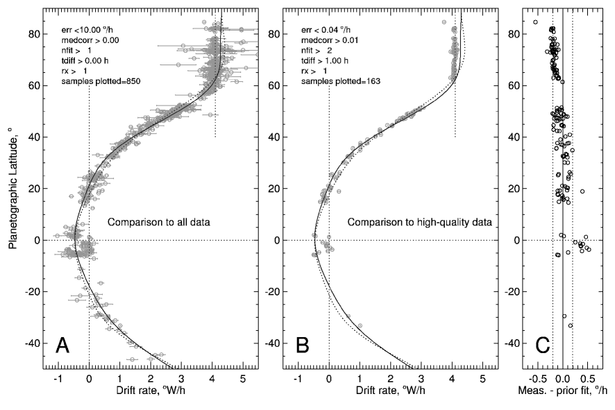
Figure 7.— Longitudinal drift rates for correlation tracking of cloud targets from 2012-2014 data sets. The full data set is in A, the subset of measurements with estimated error less than 0.04^∘/h in B, both in comparison with Model S13A (solid curve) of Sromovsky et al. (2012c), and the deviation of high-accuracy observations in B from the prior wind profile is shown in C. The dotted curves in A and B trace the S13A fit profile reflected about the equator to illustrate its hemispheric asymmetry. Note that the dotted curve north of 50^∘N comes from the solid curve south of 50^∘S latitude, which is not well constrained by observations. Sromovsky et al. (2012c) constrained the profile in this region using a single Voyager data point near 70^∘S (71^∘S planetographic), an assumed value of 4.3^∘/h westward at the south pole, and the smoothing effects of a finite number of terms fitting mainly data at other latitudes.

3.4. Binned wind results

Selecting only the high-accuracy observations leaves significant gaps in latitude coverage. To fill in those gaps we average observations within latitude bins, using the estimated variance of each observation as its weight in computing a weighted average. The results for 2^∘ bins are shown in Fig. 8 and tabulated in Tables 3 and 4. This procedure does indeed fill in many of the missing latitudes in the high-accuracy subset. The estimated error of the weighted average measurements is so small in most bins that it is within the plotted symbol. The region of solid body rotation is seen to be very uniform in these binned results. Between 65^∘ N and 83^∘ N, we obtain an average of the binned measurements of 4.079^∘/h with a standard deviation of 0.015^∘/h, compared to a range of weighted average expected errors of .002-0.022^∘/h.

Near the equator, binned results display significant scatter. Just north of the equator, the binned results are in rough agreement with the old (S13A) wind profile. But just south of the equator, the high accuracy winds from small high-contrast features has dominated the winds inferred from larger scale low contrast and wave features.

An odd feature of the binned results is that the wind profile in the region from about 18^∘N to 45^∘N seems to have a sequence of stair steps of local solid body rotation extending for a few degrees with sharp, high shear transitions between them. It could very well be the case that the zonal wind profile of Uranus is simply not a very smooth function of latitude. We also tried binning at 1^∘ intervals, and found the same stair-step structure between 10^∘N and 30^∘N, but hints of that structure at other latitudes were no longer evident, perhaps due to increased variability. The north polar region of solid-body rotation was largely unchanged by reducing the bin size, except for small increases in noise due to reduced numbers of samples per bin. No fundamentally new structures (that could be distinguished from noise) were found in the wind profile by using smaller bin sizes of 1^∘ or 0.5^∘.

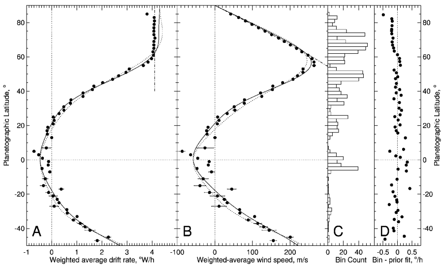
Figure 8.— Weighted-average longitudinal drift rates for correlation tracking of cloud targets from 2012-2014 data sets, averaged in 2^∘ bins (A), corresponding wind speeds (B), the number of measurements/bin (C), and differences (D) from Model S13A of Sromovsky et al. (2012c). The dotted curves in A and B are the prior profile reflected about the equator to illustrate its hemispheric asymmetry. The dot-dash lines in C and D are lines of constant angular drift rate at 4.1^∘/h. Note that both binned wind values and differences are computed at weighted average latitudes for features within the bins, not at the central latitude of the bin.

Table 3Binned 2012-2014 wind observations for the northern hemisphere.

Planetographic bin latitude			Drift rate	Std. Dev.	Wind Speed	Bin
Center	Avg.	Std. Dev.	∘E/h	∘/h	m/s	Count
85	84.58	0.41	-3.801$\pm$0.022	0.32	42.0$\pm$0.2	2
83	82.24	0.44	-4.085$\pm$0.003	0.13	63.1$\pm$0.1	12
81	80.84	0.32	-4.096$\pm$0.002	0.39	81.2$\pm$0.0	9
79	78.23	0.15	-4.081$\pm$0.015	1.00	98.7$\pm$0.4	6
77	76.11	0.58	-4.070$\pm$0.002	0.36	116.0$\pm$0.1	11
75	75.16	0.69	-4.068$\pm$0.007	0.31	133.3$\pm$0.2	24
73	73.51	0.50	-4.074$\pm$0.004	0.26	150.7$\pm$0.1	48
71	71.00	0.60	-4.114$\pm$0.008	0.52	169.4$\pm$0.3	12
69	68.74	0.66	-4.072$\pm$0.006	0.28	184.5$\pm$0.3	23
67	66.93	0.64	-4.068$\pm$0.004	0.18	200.8$\pm$0.2	51
65	65.23	0.59	-4.067$\pm$0.005	0.24	217.0$\pm$0.3	49
63	63.41	0.51	-4.035$\pm$0.004	0.22	231.2$\pm$0.2	39
61	61.30	0.49	-4.050$\pm$0.009	0.18	247.7$\pm$0.6	22
59	59.11	0.56	-3.979$\pm$0.017	0.14	258.3$\pm$1.1	21
57	57.33	0.43	-3.841$\pm$0.017	0.15	263.4$\pm$1.1	22
55	55.16	0.41	-3.651$\pm$0.057	0.07	263.5$\pm$4.1	3
53	52.34	0.18	-3.094$\pm$0.023	0.15	234.2$\pm$1.7	11
51	50.77	0.48	-2.959$\pm$0.005	0.20	234.0$\pm$0.4	45
49	48.42	0.50	-2.665$\pm$0.005	0.23	219.5$\pm$0.4	46
47	47.34	0.54	-2.426$\pm$0.003	0.22	207.6$\pm$0.2	40
45	44.54	0.53	-2.031$\pm$0.004	0.16	180.0$\pm$0.3	17
43	42.38	0.57	-1.681$\pm$0.002	0.22	154.0$\pm$0.2	11
41	40.95	0.41	-1.620$\pm$0.012	0.15	153.0$\pm$1.1	15
39	39.05	0.46	-1.250$\pm$0.000	0.11	121.4$\pm$0.0	17
37	37.67	0.53	-1.248$\pm$0.000	0.19	124.5$\pm$0.0	25
35	35.60	0.34	-0.771$\pm$0.001	0.13	78.8$\pm$0.1	12
33	33.43	0.53	-0.748$\pm$0.001	0.14	78.3$\pm$0.1	21
31	30.14	1.07	-0.482$\pm$0.012	0.13	51.5$\pm$1.3	4
29	28.89	0.21	-0.487$\pm$0.054	0.15	53.1$\pm$5.9	3
27	26.26	0.26	-0.297$\pm$0.020	0.15	32.9$\pm$2.3	4
25	25.21	0.53	-0.065$\pm$0.000	0.17	7.4$\pm$0.0	26
23	23.27	0.62	-0.097$\pm$0.017	0.33	11.1$\pm$2.0	11
21	20.38	0.53	-0.058$\pm$0.004	0.17	6.7$\pm$0.5	13
19	19.19	0.51	0.155$\pm$0.000	0.22	-18.2$\pm$0.0	12
17	17.05	0.64	0.184$\pm$0.000	0.15	-21.8$\pm$0.0	14
15	15.70	0.62	0.173$\pm$0.001	0.16	-20.7$\pm$0.1	6
13	12.85	0.56	-0.003$\pm$0.034	0.09	0.4$\pm$4.1	3
7	6.17	0.00	0.214$\pm$0.193	0.00	-26.3$\pm$23.7	1
5	5.04	0.39	0.703$\pm$0.063	0.12	-86.8$\pm$7.8	3
3	2.31	0.74	0.519$\pm$0.017	0.12	-64.3$\pm$2.2	11
1	1.51	0.41	0.367$\pm$0.014	0.23	-45.5$\pm$1.7	20

Table 4Binned 2012-2014 wind observations for the southern hemisphere.

Planetographic bin latitude			Drift rate	Std. Dev.	Wind Speed	Bin
Center	Avg.	Std. Dev.	∘E/h	∘/h	m/s	Count
-3	-3.02	0.74	0.139$\pm$0.011	0.30	-17.2$\pm$ 1.4	17
-5	-5.38	0.48	0.383$\pm$0.009	0.23	-47.3$\pm$ 1.1	39
-7	-6.49	0.45	0.072$\pm$0.063	0.36	-8.8$\pm$ 7.7	4
-11	-11.30	0.00	0.255$\pm$0.116	0.00	-31.1$\pm$14.1	1
-15	-14.60	0.00	0.328$\pm$0.130	0.00	-39.4$\pm$15.6	1
-17	-16.68	0.00	-0.379$\pm$0.099	0.00	45.0$\pm$11.8	1
-19	-18.56	0.00	0.121$\pm$0.113	0.00	-14.2$\pm$13.3	1
-21	-21.24	0.35	-0.060$\pm$0.168	0.36	6.9$\pm$19.5	2
-23	-23.36	0.47	-0.221$\pm$0.044	0.37	25.3$\pm$5.1	3
-25	-24.55	0.56	-0.293$\pm$0.042	0.25	33.0$\pm$4.7	3
-27	-26.03	0.00	-0.101$\pm$0.178	0.00	11.2$\pm$19.7	1
-29	-29.43	0.41	-0.603$\pm$0.018	0.19	65.7$\pm$2.0	5
-31	-30.61	0.45	-0.622$\pm$0.033	0.11	66.4$\pm$3.5	4
-33	-33.17	0.82	-1.010$\pm$0.005	0.19	105.7$\pm$0.5	2
-35	-34.67	0.25	-0.869$\pm$0.071	0.20	88.8$\pm$7.2	2
-37	-36.06	0.00	-1.140$\pm$0.110	0.00	113.8$\pm$11.0	1
-39	-39.78	0.00	-1.333$\pm$0.105	0.00	129.6$\pm$10.2	1
-41	-41.31	0.00	-1.526$\pm$0.198	0.00	144.2$\pm$18.7	1
-45	-44.50	0.15	-2.262$\pm$0.093	0.17	200.5$\pm$8.2	2
-47	-46.22	0.11	-1.816$\pm$0.101	0.24	155.4$\pm$8.7	2

3.5. The problem of measuring near-equatorial wind speeds

Very few compact discrete cloud features have ever been observed in the near-equatorial region (within about 10^∘ of the equator). Most of the zonal drift rates in this region have been estimated by tracking wave features, either the ribbon wave that can be seen near 5^∘S in the most of the high S/N images, or diffuse bright features that also seem to be associated with waves. An unusual appearance of compact discrete cloud features in the 2014 images in the 0-5^∘S region provided a distinctly different drift rate estimate that is close to zero. Which of these is the best estimate of the atmospheric mass flow is not certain, although waves are often seen traveling relative to the mass flow. Thus we tend to favor the small discrete clouds as more representative of the mass flow. On the other hand, the only independent measure of the mass flow, inferred from radio occultation measurements (Lindal et al. 1987) suggests that the mass flow is more eastward than either the wave or discrete feature results, although the measurement has such a large error bar that it does not provide a very firm constraint.

4. Legendre polynomial fits and symmetry properties

4.1. Legendre fitting methodology

Our aim in carrying out polynomial fits to the wind observations was to provide a smooth profile for atmospheric modelers and other researchers. We modeled longitudinal drift rates and wind speeds using the following Legendre expansion and conversion equations:

$$d\phi/dt=\sum_{i=0}^{n}C_{i}\times P_{i}(\sin(\theta))$$ (2)

$$U=-4.8481\times 10^{-3}R(\theta)\times d\phi/dt$$ (3)

$$R(\theta)=R_{E}/\sqrt{1+(R_{P}/R_{E})^{2}\tan(\theta)^{2}}$$ (4)

where $C_{i}$ are the coefficients given in Table 5, $P_{i}(\sin(\theta))$ is the $i$th Legendre polynomial evaluated at the sine of planetographic latitude $\theta$, $d\phi/dt$ is the longitudinal drift rate in ^∘/h (using planetographic longitude, which is east longitude for a retrograde rotator like Uranus), $U$ is the westward wind speed in m/s, $R$ is the radius of rotation in km at latitude $\theta$, which is the distance from a point on the 1-bar surface to the planet’s rotational axis, and $R_{E}$ and $R_{P}$ are the equatorial and polar radii of Uranus, for which we use 25559 km and 24973 km (Archinal et al. 2011). We fit the longitudinal drift rates rather than wind speeds, because the former do not change as dramatically at high latitudes as the latter, and thus are much easier to fit without generating large deviations in data-sparse latitude regions. To limit such large deviations, we also need to limit the order of the polynomials. For the symmetric fits, the summation over $i$ is only over the even polynomials. The model coefficients are found by minimizing $\chi^{2}$, but with error estimates for the observations modified as described by Sromovsky et al. (2012c) and paraphrased in the following paragraph. Note that while we tabulate drift rates in east longitude, the plots show westward drift rates to be consistent with the prior practice of making prograde (in this case westward) winds positive (Allison et al. 1991; Hammel et al. 2001, 2005; Sromovsky and Fry 2005; Sromovsky et al. 2009).

Because very accurate measurements of drift rates at nearly the same latitude often differ by many times the value expected from those uncertainties, it appears that one or more of the following must be true: (1) the circulation is not entirely steady, (2) the features that we measure do not all represent the same atmospheric level, (3) the feature tracked has evolved or been misidentified, or (4) the cloud features we track are not always at the same latitude as the cloud-generating circulation feature that is moving with the zonal flow. Examples of the latter possibility are the companion clouds to Neptune’s Great Dark Spot (Sromovsky et al. 1993). In Section 5.2.1 we provide examples from our current data set. If we weighted highly accurate measurements by their expected inverse variance, they would dominate the fit, leading to wild variations in regions where there are less accurate measurements. Since these high accuracy measurements clearly do not all follow the mean flow, we must add an additional uncertainty to characterize their deviations from it. We do this by root sum squaring the estimated error of measurement with an additional error of representation denoted by $\sigma_{R}$, which is adjusted so that the $\chi^{2}$ value of the complete fit is approximately equal to the number of measurements. The need for $\sigma_{R}$ might be partly due to slight discrepancies in latitude that arise from a cloud feature being generated by a circulation feature that is latitudinally offset from the bright cloud feature that is tracked.

Another factor in evaluating wind measurement accuracy is the rate at which latitudinal accuracy and drift rate accuracy improve with extended tracking time spans. Drift rate accuracy improves roughly linearly with time span, and can improve dramatically from just a few widely separated measurements, while latitude accuracy improves as the square root of the number of measurements, and is not much improved by adding just a few measurements or by extending the time span of the measurements. If we consider a shear of 2^∘/h per 10^∘ of latitude (about the maximum observed shear), a half-degree error in latitude is equivalent to a 0.1^∘/h error in wind measurement, which is about the value of $\sigma_{R}$ that we need to make the $\chi^{2}$ value for the fit equal to the number of degrees of freedom (or $\chi^{2}$/N_F $\approx$ 1). The apparent local stair steps suggested by the binned wind profile would also cause local errors relative to a smooth profile. We found $\sigma_{R}\approx$ 0.1^∘/h for both the 2009-2011 and 2007-2011 data sets analyzed by Sromovsky et al. (2012c). A similar value was needed in our current analysis.

4.2. Symmetric fit results

Because our 2012-2014 wind data set contains such a sparse sampling of the southern hemisphere, with no samples poleward of 47^∘S, it is difficult to reliably constrain any north-south asymmetry in the wind profile. Accordingly, we first considered fits using a series of even Legendre polynomials, which guarantees hemispheric symmetry and provides a useful reference for detecting asymmetries. To fit the relatively sharp kinks near 55^∘N and 62^∘ N, we needed to use a fairly large number of polynomials. After finding fit problems with orders of 10-14, we settled on a ten-term series of even polynomials up to order 18. The results are shown in Fig. 9 for the case in which we fit essentially the entire data set, including 846 measurements and eliminating only 6. This is shown as a solid line, while the most recent fit to prior observations, Model S13A, is shown as a dotted line. Here we also added synthetic points at both north and south poles to help straighten out our drift rate fit at high northern polar latitudes. We used a $\sigma_{R}$ value of 0.147^∘/h. The Legendre coefficients and their uncertainties are given in Table 5. There we also provide coefficients for alternate fits discussed later in this section.

In comparison with our new symmetric fit, the prior asymmetric fit provides a degree of asymmetry in the 20^∘ - 40^∘ range that seems to provide slightly better agreement with the new observations in that region. But in the region from 55^∘N to 85^∘N, the old fit has a solid body rotation rate that is 0.2^∘/h too fast. This might represent a slight decrease over time, but the small number of 2011 measurements and their error bars of 0.3^∘/h or more, make this a difference of dubious significance. Near the equator, our new fit has a lower eastward drift rate, which is a result of the large number of high quality 2014 measurements between -6^∘ and 1^∘ that pull the profile closer to zero. Our new fit is not quite straight enough to fit the constant rotation rate observed at high northern latitudes, but is within about 0.1^∘/h of the correct drift rate. Near the equator, this fit splits the difference between small discrete results and the large pattern results. This leads to a nearly solid body rotation within about 7.5^∘ of the equator, at a rate of about 0.12^∘ /h eastward.

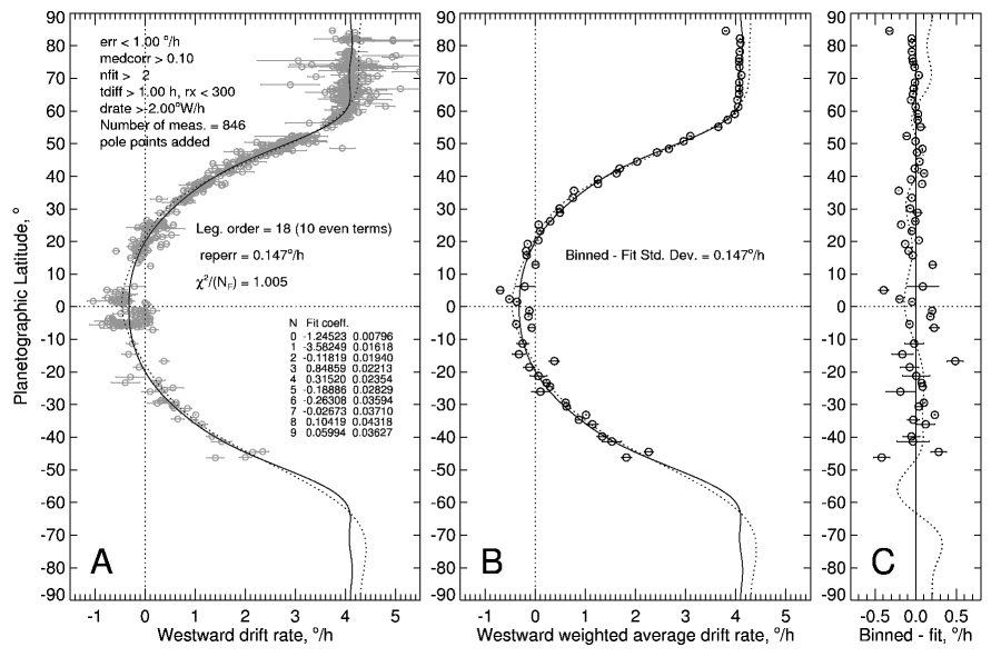
Figure 9.— Ten-term order-18 Legendre polynomial fit to nearly our entire data set using a $\sigma_{R}$ (reperr) value of 0.147^∘/h, which is shown as a solid curve, in comparison with our large data set in (A) and with our binned data set in (B). The difference between binned results and the fit are shown in C. The dotted curves in A and B show Model S13A of Sromovsky et al. (2012c).

An alternative fit that eliminates the high-correlation low-latitude 2014 observations (those associated with small discrete features), but leaving the drift rates derived from wave features, is shown in Fig. 10A. For this fit we reduced $\sigma_{R}$ to 0.128^∘/h. This fit displays a clear retrograde (eastward) equatorial peak. Realizing that the observations near 6^∘ S and near 2^∘ N, with drift rates less than -0.3^∘/h are measurements of wave motions, while the 2014 measurements in this region are almost entirely of small discrete features that are more likely indicators of mass flow, we also carried out a fit in which the putative wave tracking results are eliminated. That fit, displayed in Fig. 10B, contains a region within 15^∘ of the equator that appears to be in solid body rotation at a rate of 0.1^∘/h eastward.

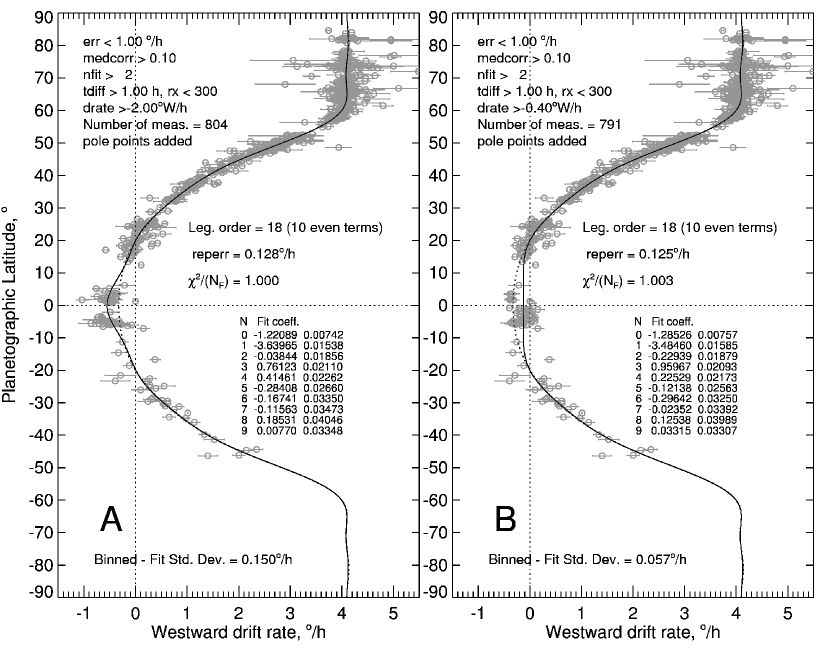
Figure 10.— As in Fig. 9, except that (A) 2014 measurements of discrete features between 7^∘S and 2^∘N are excluded from the fit, and a $\sigma_{R}$ (reperr) of 0.15^∘/h was used, and for (B) observations of near equatorial wave motions were excluded from the fit, and a $\sigma_{R}$ = 0.125^∘/h was used. The fits are shown by solid lines, while the dotted line here shows the fit that includes all the data.

Table 5Fit coefficients for symmetric Legendre polynomial fits to 2012-2014 wind observations.

	Legendre	Fit 1 (846 pts)		Fit 2 (Eq. spots excl.)		Fit 3 (Eq. waves excl.)
Term	Order	Coeff.	Unc.	Coeff.	Unc.	Coeff.	Unc.
0	0	-1.245225	0.0079	-1.220885	0.0074	-1.285259	0.0076
1	2	-3.582487	0.0162	-3.639650	0.0154	-3.484602	0.0158
2	4	-0.118185	0.0194	-0.038439	0.0186	-0.229385	0.0188
3	6	0.848593	0.0221	0.761227	0.0211	0.959671	0.0209
4	8	0.315199	0.0235	0.414609	0.0226	0.225287	0.0217
5	10	-0.188857	0.0283	-0.284082	0.0266	-0.121381	0.0256
6	12	-0.263077	0.0359	-0.167412	0.0335	-0.296423	0.0325
7	14	-0.026728	0.0371	-0.115626	0.0347	-0.023522	0.0339
8	16	0.104192	0.0432	0.185315	0.0405	0.125384	0.0399
9	18	0.059944	0.0362	0.007696	0.0335	0.033149	0.0331

4.3. Evidence for mid-latitude asymmetry

The very small asymmetry we see in the 2012-2014 observations is interesting to compare with prior observations of Uranus. As shown in Fig. 11, the strongest indication of mid-latitude asymmetry comes from observations made between 1997 and 2005, which are based on HST imaging (Karkoschka 1998; Hammel et al. 2001) and Keck imaging (Hammel et al. 2001; Sromovsky and Fry 2005; Sromovsky et al. 2007; Hammel et al. 2009; Sromovsky et al. 2009). The dotted curve in this figure is the sum of our symmetric fit and the all-data asymmetric fit to the differences from the symmetric fit, described later in the section and shown in the left panel of Fig. 12. Observations from 2007 Keck imaging (Sromovsky et al. 2009) and 2009 HST imaging (Fry et al. 2012a) are in close agreement with 2012-2014 results. The 2011 results (Sromovsky et al. 2012c) from Keck and Gemini imaging, provide insufficient mid-latitude sampling to constrain the asymmetry properties of the circulation on their own, but they do contribute to the impression that there is indeed an asymmetry. This is made more apparent by the plots of measurements relative to the symmetric model in Fig. 12. There we also plot a simple model that provides a crude fit to the residuals. We considered two empirical models of the asymmetry. To fit the asymmetry average for all the high-quality observations from Voyager through 2014, we used the following model:

$$d\phi/dt(\theta)=A\times(-|(\theta)|/\theta))\exp(-((\theta-b)/c)^{2})$$ (5)

where we found $A$=0.085^∘/h to be the best-fit amplitude, $b$=29^∘ to be the best-fit peak location in latitude, and $c$=10.5^∘ to be the best-fit latitudinal width parameter. The second factor in Eq. 5 provides the sign reversal between hemispheres and is replaced by zero at the equator. A comparison of our fit to the observations can be found in Fig. 12 (left panel). Measurements prior to 2012-2014 suggest a larger and more complex asymmetry structure, which we fit using the following model:

$$d\phi/dt(\theta)=A\sin[2\pi(\theta/a)]\exp(-((\theta-b)/c)^{2})$$ (6)

where in this case $A$=0.135^∘/h provides the best-fit asymmetry amplitude, $a$=40.5^∘provides the best latitudinal period of variation, $b$= 35^∘ the best peak of the exponential factor, and $c$=19.5^∘ the best damping width of the exponential. These parameters are only crudely constrained by the observations, as can be seen from a comparison of this model with the difference plots in Fig. 12 (right panel).

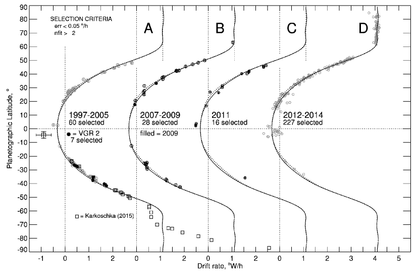
Figure 11.— Higher accuracy wind measurements from 1997-2005 (A), 2007-2009 (B), 2011 (C), and 2012-2014 (D), compared to our new even polynomial fit to the entire 2012-2014 data set (solid curves). In (A) we also show Voyager 2 observations Smith et al. (1986) as filled black circles and one radio occultation result (large square) from Lindal et al. (1987), as well as the discrete tracking results (small squares) from the reanalysis of Voyager 2 images by Karkoschka (2015). See text for further references. The dotted curves are the sum of the even (symmetric fit) and the asymmetric fit to the differences, as shown in the left panel of Fig. 12.

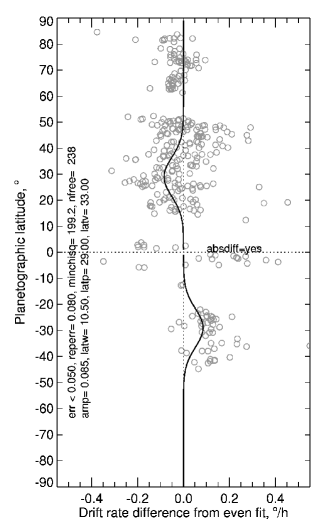
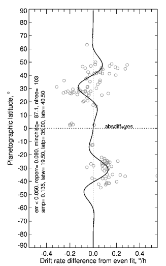
Figure 12.— Wind difference between our symmetric model and all measurements shown in Fig. 11 (Left) and differences excluding 2012-2014 observations (Right). Simple best-fit models are shown by solid lines. The left fit uses an asymmetric Gaussian and the right fit uses a damped sine function (both defined in the text). To reduce the impact of outliers, both fits minimized the sum of absolute differences scaled by expected errors. The earlier observations seem to have somewhat more pronounced asymmetry.

4.4. Comparison with new southern winds from Voyager

Voyager approached Uranus in 1986, when the southern hemisphere was facing the sun, but very few winds were obtained because very few cloud features were detected. Recently, Karkoschka (2015) carried out an extensive reprocessing of Voyager imagery to remove artifacts, improve non-linearity corrections, and carry out shift-and-add averaging, similar to the high S/N approach we used in our analysis, except that many more images were averaged and much higher S/N ratios were achieved, allowing the detection of very low contrast cloud patterns and discrete cloud features over most of the southern hemisphere. Twenty-seven discrete cloud features were tracked between 87^∘S and 23.6^∘S. These are shown in Fig. 13 in comparison to the asymmetric profile of Sromovsky et al. (2012c) and to southern hemisphere measurements from our 2012-2014 data set. Also shown is the result of Karkoschka’s correlation tracking at 395 latitudes between the equator and the pole. These new results are in generally good agreement with current and prior results north of 55^∘S, where the non-Voyager results exist. But there are many substantial deviations and remarkable asymmetries implied by the new results, as discussed in the following paragraphs.

First, we consider the correlation tracking results (small black dots in Fig. 13). These show regions of constant longitudinal drift rate, or solid-body rotation (26^∘S - 36^∘S, 36^∘S - 42^∘S, and 58^∘S - 68^∘S, for example). The regions north of 50^∘S are not in agreement with prior measurements, as shown in Fig. 14, most of which follow a smooth variation with latitude. Exceptions are probably due to the fact that larger vortex features can generate cloud features over a range of latitudes that travel along with the generating feature rather than following the zonal wind profile. Major examples of this effect are provided by the Great Dark Spot and other dark spots on Neptune (Sromovsky et al. 2002). We also identify a pair of uranian features with this characteristic in Section 5.2.1. Thus, it is conceivable that, at least where we have contradicting observations, the regions where Karkoschka’s Voyager correlation results show solid-body rotation are due to large circulation features that influence an extended latitude region, generating clouds that travel with the circulation features rather than following the zonal flow. This is less plausible as an explanation for the 58^∘S to 68^∘S region because of its size. While we find small regions of apparent solid body rotation in our data set in the northern hemisphere, these are not as extensive as the mid-latitude regions in Karkoschka’s correlation profile. The major region of solid body rotation that we find, from 62^∘N to 83^∘N, is clearly not an artifact, as it is based on numerous well-defined discrete cloud features. There is an amazing amount of shear in Karkoschka’s correlation profile, just where one solid body region transitions to another. When plotted as wind speeds, there regions of enormous jumps in wind speed over a very short distance, zig-zagging to higher values as latitude increases toward the pole, then decreasing for a while, then jumping again to a new high. This characteristic also suggests that these features might not represent the zonal wind structure.

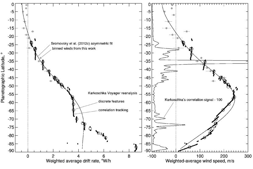
Figure 13.— Southern hemisphere longitudinal drift rates (left) and corresponding wind speeds (right) obtained from reanalysis of 1986 Voyager images by Karkoschka (2015), compared to the asymmetric fit (solid curve) of Sromovsky et al. (2012c) and our measurements from 2012-2014 observations (gray dots). Two Karkoschka results are shown: tracking of discrete cloud features (open circles) and correlation tracking of patterns in narrow latitude bands (small black dots). Also plotted at the right is the Karkoschka correlation signal-100 versus latitude, where the signal unit is 10^-5 in I/F. Only points above correlation signals of 6 are shown, due to scatter obtained for lower signal levels.

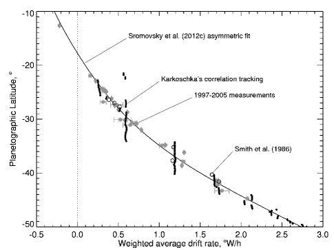
Figure 14.— The Karkoschka (2015) correlation tracking results (small black dots), compared to the asymmetric fit (solid curve) of Sromovsky et al. (2012c), 1997-2005 measurements (larger gray dots), and prior Voyager results (open circles) of Smith (1986). The uncertainty in the latter results is comparable to the size of the plotted symbols, while error bars are shown for 1997-2005 measurements.

The most extraordinary result from Karkoschka (2015) is the huge north-south asymmetry it implies at high latitudes. Between 70^∘S and 87^∘S, his inferred westward drift rates rises from 3.8^∘/h to 8.6^∘/h, which is more than double what we measured at high northern latitudes, where drift rates are invariant with latitude over a comparable latitude range. Given that the middle latitude winds have changed by barely measurable amounts from 1986 through 2014, a 28-year period, it is hard to understand how such enormous seasonal changes might occur. If the north-south difference is seasonal, and the Voyager analysis represents the winds at the southern summer solstice (October 6, 1985), then we would expect that the same wind profile would appear in northern latitudes by the time of the northern summer solstice in 2030 (on April 29 according to Meeus (1997)). That is less than 16 years over which this enormous change should occur, while almost nothing has changed at middle latitudes in the last 28 years. Evidence for change at high latitudes is only beginning to be accumulated. There may have been a small decrease in the solid body rotation rate from 4.3^∘/h to 4.1^∘/h between 2011 and 2014, but that is probably within the error of the 2011 measurements, and provides little evidence for the rapid change needed to match in 2030 what seems to have existed in 1986 in the southern hemisphere, according to Karkoschka (2015). On the other hand, perhaps this north-south difference is a permanent feature of the wind profile, just as it appears that Jupiter and Saturn have asymmetries that survive over a complete change of seasons. It will certainly be worthwhile to monitor the winds of Uranus over the next two decades to determine whether this asymmetry is really a seasonal effect.

4.5. A complete zonal profile for Uranus

Here we create a complete pole-to-pole zonal wind profile for Uranus by combining results from groundbased observations at latitudes spanning 47^∘S to 83^∘N with the recent Karkoschka (2015) results for the southern hemisphere, obtained from 1986 Voyager 2 imaging. In Fig. 15 we show our composite profile in comparison with binned observations and the discrete cloud tracking results of Karkoschka (2015). The composite profile uses our symmetric fit to our 2012-2014 observations (Fig. 9) summed with the asymmetric fit to differences from that profile, as displayed in Fig. 12A, to cover the latitude range from 46^∘S to 67^∘N. From 67^∘N to 90^∘N we used a solid-body rotation profile of 4.1^∘/h westward. From 47^∘ S to 90^∘S we used the adopted profile of Karkoschka (2015). The latter profile does not pass exactly through the discrete measurements in this region, probably because the profile also took into account correlation measurements. The composite profile is also provided in Tables 6 and 7. This represents our best estimate of the zonal wind profile of Uranus under the assumption that the indicated asymmetry is a permanent feature of the atmosphere. This may be an incorrect assumption. Since the southern winds from Voyager are based on 1986 observations, while the remaining winds (from 47^∘S to 90^∘N) are based on observations heavily weighted towards the 2012-2014 time period, this may not represent the current profile.

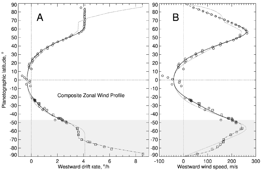
Figure 15.— Composite zonal profiles of longitudinal drift rate (A) and wind speed (B) versus latitude. The grayed region from 47^∘S to 90^∘S is where we used the adopted profile of Karkoschka (2015), which is based on his reanalysis of 1986 Voyager images (dot-dash curve). The adopted profile for higher latitudes (solid curve) is based on a symmetric fit to the 2012-2014 observations defined in Fig. 9 and the asymmetry fit to all selected observations defined in Fig. 12A. One exception is that we replaced the nearly constant angular velocity region north of 67^∘N with an exactly constant profile (dashed line). In each panel the dotted curve gives the adopted profile reflected about the equator, which shows the degree of north-south asymmetry that is present. Also shown are binned results from the current work (open circles) and discrete cloud tracking results from Karkoschka (2015). Our adopted profile is also given in Tables 6 and 7.

Table 6Adopted westward drift rate (D) profile in ^∘/hour vs. planetographic latitude (L).

L, ∘	D(L)	D(L-1)	D(L-2)	D(L-3)	D(L-4)	D(L-5)	D(L-6)	D(L-7)	D(L-8)	D(L-9)
90	4.100	4.100	4.100	4.100	4.100	4.100	4.100	4.100	4.100	4.100
80	4.100	4.100	4.100	4.100	4.100	4.100	4.100	4.100	4.100	4.100
70	4.100	4.100	4.100	4.100	4.097	4.100	4.099	4.090	4.072	4.043
60	4.002	3.946	3.875	3.789	3.687	3.571	3.443	3.302	3.153	2.997
50	2.836	2.673	2.510	2.349	2.191	2.039	1.893	1.753	1.620	1.493
40	1.373	1.258	1.149	1.045	0.946	0.850	0.759	0.672	0.588	0.509
30	0.434	0.363	0.298	0.237	0.181	0.129	0.083	0.040	0.002	-0.032
20	-0.064	-0.092	-0.118	-0.142	-0.164	-0.185	-0.204	-0.222	-0.238	-0.253
10	-0.266	-0.278	-0.289	-0.298	-0.305	-0.312	-0.317	-0.321	-0.323	-0.325
0	-0.325	-0.324	-0.322	-0.319	-0.314	-0.308	-0.300	-0.290	-0.278	-0.264
-10	-0.247	-0.228	-0.206	-0.181	-0.154	-0.124	-0.090	-0.054	-0.015	0.027
-20	0.072	0.120	0.170	0.223	0.278	0.335	0.394	0.455	0.518	0.582
-30	0.647	0.714	0.783	0.854	0.927	1.002	1.081	1.164	1.253	1.346
-40	1.447	1.554	1.669	1.793	1.924	2.064	2.210	2.359	2.501	2.645
-50	2.790	2.937	3.086	3.166	3.247	3.328	3.410	3.492	3.575	3.578
-60	3.581	3.585	3.588	3.591	3.595	3.598	3.601	3.605	3.608	3.749
-70	3.891	4.035	4.181	4.328	4.596	4.869	5.120	5.377	5.638	5.904
-80	6.250	6.605	6.970	7.344	7.729	8.124	8.530	8.530	8.530	8.530
-90	8.530

Table 7Adopted westward zonal wind (U) profile in m/s vs. planetographic latitude (L).

L, ∘	U(L)	U(L-1)	U(L-2)	U(L-3)	U(L-4)	U(L-5)	U(L-6)	U(L-7)	U(L-8)	U(L-9)
90	0.00	9.07	18.15	27.21	36.27	45.31	54.34	63.35	72.33	81.29
80	90.23	99.13	108.00	116.83	125.62	134.36	143.06	151.72	160.32	168.86
70	177.35	185.77	194.14	202.43	210.53	218.84	226.82	234.33	241.20	247.23
60	252.26	256.13	258.70	259.87	259.57	257.78	254.54	249.90	243.99	236.94
50	228.93	220.13	210.74	200.94	190.88	180.72	170.58	160.54	150.67	140.99
40	131.53	122.27	113.20	104.30	95.56	86.97	78.54	70.28	62.22	54.39
30	46.83	39.60	32.73	26.26	20.20	14.58	9.40	4.63	0.26	-3.75
20	-7.43	-10.82	-13.96	-16.88	-19.60	-22.16	-24.55	-26.78	-28.85	-30.75
10	-32.49	-34.05	-35.43	-36.63	-37.64	-38.49	-39.16	-39.67	-40.02	-40.22
0	-40.24	-40.11	-39.85	-39.42	-38.81	-37.99	-36.95	-35.66	-34.12	-32.29
-10	-30.17	-27.74	-24.99	-21.92	-18.53	-14.81	-10.77	-6.41	-1.76	3.19
-20	8.41	13.87	19.57	25.47	31.55	37.76	44.08	50.48	56.92	63.39
-30	69.87	76.35	82.83	89.33	95.88	102.50	109.26	116.20	123.37	130.83
-40	138.62	146.78	155.32	164.22	173.44	182.92	192.53	201.83	210.02	217.83
-50	225.25	232.26	238.84	239.62	240.08	240.23	240.04	239.52	238.66	232.26
-60	225.77	219.19	212.53	205.78	198.95	192.04	185.05	177.98	170.85	169.86
-70	168.32	166.19	163.48	160.17	160.37	159.58	156.88	153.20	148.50	142.75
-80	137.54	130.97	122.96	113.47	102.43	89.78	75.45	56.61	37.75	18.88
-90	0.000

5. Persistent cloud patterns and discrete features

A number of discrete features and cloud patterns were found to persist for long time periods. To facilitate their identification we created a mosaic of high S/N H-filter images for each high-resolution data set for which successive observing nights allowed us to take multiple images of both sides of the planet, totaling between 144 and 179 images per data set. This made it possible to combine all longitudes into one rectangular map. Overlapping images were blended with a weighting of $\mu^{2}T/T_{\circ}$, where $\mu$ is the observer zenith angle cosine and $T/T_{\circ}$ is the image exposure ratio. Also, pixels were mosaicked only if $\mu$ and $\mu_{\circ}$ (solar incidence angle cosine) were greater than or equal to 0.025. These two cosines are so close together that a Minnaert model of brightness variation, i.e. $I\mu=I_{\circ}(\mu\mu_{\circ})^{k}$, which is fit well with $k=0.6$ for H-filter images, collapses to $I=I_{\circ}\mu^{0.2}$. Because this is a such a weak dependence on view angle we did not attempt to correct for it. High-pass filtered versions of these mosaics are shown as rectangular projections in Fig. 16 at a scale 0.25^∘/pixel. These were obtained by subtracting from the mosaicked images a version smoothed with a 6.25^∘ (25-pixel) boxcar average. To display the resulting low-contrast variations, we enhanced these images so that black and white respectively correspond to I/F deviations of -0.4$\times 10^{-4}$ and +0.8$\times 10^{-4}$ from the smoothed versions, which have a central disk I/F of about 0.01. The combination of images taken at different times requires that each longitudinal image line from each component image be shifted by the zonal wind drift rate times the time difference between the image time and the reference time of the map (chosen to be the midpoint of the observations for the two nights). This does not distort features at low and high latitudes, because wind shear is very low at low latitudes and zero above 55^∘N. However, at middle latitudes (25-55^∘), where wind shear is significant, round features become stretched into slanted ellipses. This distortion is a reasonable price to pay for obtaining a global view of where features are located and how many features are present in a given band of latitude. For key features that are identified, we also provide in the following section undistorted views that more accurately display morphological characteristics.

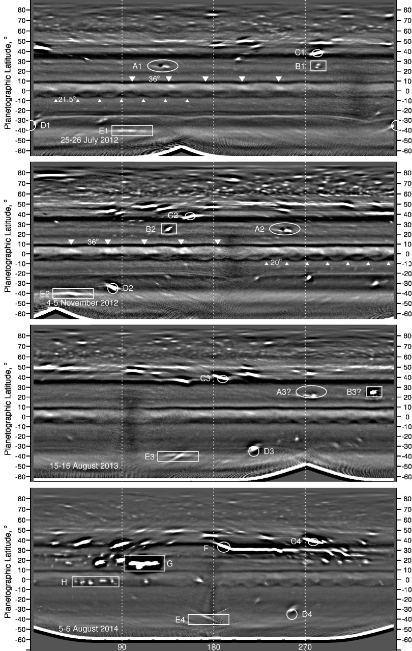
Figure 16.— Rectangular projections of 2-night mosaics from July 2012 (top), November 2012, August 2013, and August 2014 (bottom). Each is high-pass filtered so that low-contrast features could be enhanced without being overwhelmed by brightness variations as a function of latitude (see text).

5.1. Discrete feature identification based on morphology

Inspecting the four rectangular maps in Fig. 16, we see that there are too many features of similar appearance in the north polar region to identify which, if any, might have lasted for long time periods. The band from 45^∘N to 50^∘N also has too many features to make any unambiguous matches between data sets. In other, less populated regions, we were able to identify six discrete long-lived features (A-F), which are also shown enlarged and without high-pass filtering in Fig. 17.

Between 20^∘N and 30^∘N, only two significant features are seen in July 2012 (A1 and B1), November 2012 (A2 and B2), and August 2013 (A3 and B3). A1 and A2 have nearly identical morphologies and latitudes ($\approx$25^∘N), making identification rather easy. In the high-pass filtered images they appear as small dark spots with what look like companion clouds traveling with them, consistent with the idea that the bright features are orographic clouds generated by vertical deflections associated with flow around an oval vortex. In this case vertical deflections cause adiabatic cooling and condensation of cloud particles. The dark feature so clearly visible in the high-pass filtered version is also apparent without such filtering, as shown in Fig. 17. Feature A3 is likely associated with the same vortex, but the morphological match is not as good, with no dark spot showing.

Feature B is at essentially the same latitude as feature A, but its bright features can be found both north and south of the bright features associated with A. From a comparison of A2 and B2 subimages in Fig. 17, we see that the bright features of B are indeed north of the bright features of A, but there seems to be a dark spot associated with B that is at a lower latitude than the dark spot associated with A. It is likely that the latitude of the dark spot is what really matters because the bright features are likely to follow the motion of the dark spot, rather than the zonal wind profile, a behavior already well established for dark spots on Neptune.

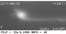
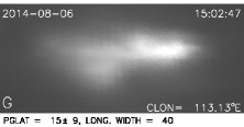
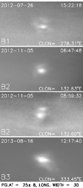
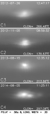
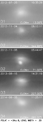
Figure 17.— Rectangular projections of discrete features A-D, F, and G. These are stretched but not high-pass filtered.

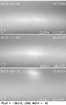
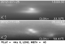
Figure 18.— Rectangular projections of discrete features E (40^∘ in longitude $\times$ 20^∘ in latitude), K (40^∘ $\times$ 12^∘), and near equatorial waves (W1-W4)(80^∘ $\times$ 20^∘). Only W1-W4 are high-pass filtered, which was needed to remove a strong latitudinal gradient in brightness.

One feature that seems to have survived at the same latitude all the way from July 2012 to August 2014, is the feature labeled C1-C4, which appears at latitude 38^∘ N.

5.2. Long-lived discrete feature tracking

To solidify the identification of discrete features, we tried to add longitudinal continuity to the morphological character and zonal uniqueness evident at several discrete times. If the features we have identified as unique are indeed the same at each time period, then their longitudes should be a continuous function of time that is roughly consistent with the zonal winds within the latitude region where they are found. During 2012 we acquired observations over a 4-month period, with a similar range covered in 2014, providing strong constraints on longitudinal and latitudinal motions, but only one sample was obtained between these times, during 15-16 August 2013.

We first tried to fit observations to the simplest model in which longitude is a linear function of time, implying that the drift rate is constant and that the latitude of the feature (or that of the circulation feature generating the visible cloud feature) is constant. None of the long-lived features followed this simple model for the entire time period. Two other models were then considered: (1) a sinusoidal variation in drift rate (and latitude), which leads to a sinusoidal variation in longitude relative to a linearly increasing longitude, and (2) a linear variation in drift rate (and a linearly increasing latitude), which implies that the longitude should vary as the square of the time difference (at least over small ranges of latitude for which a constant wind shear is a plausible assumption). The linear latitudinal drift model can be expressed as follows:

$$\phi(t)=\phi_{\circ}+a\times(t-t_{0})+b\times(t-t_{0})^{2}$$ (7)

$$\omega(t)=d\phi(t)/dt=a+2b\times(t-t_{0})$$ (8)

$$\theta(t)=\theta_{\circ}+2b\times(t-t_{0})/(d\omega/d\theta)$$ (9)

where $\phi(t)$ is longitude at time $t$, $\omega$ is rate of change of longitude, $\theta$ is latitude, and $d\omega/d\theta$ is the latitudinal shear in the zonal wind profile. The corresponding equations for the sinusoidal variation model are as follows:

$$\phi(t) = \phi_{\circ}+a\times(t-t_{0})+c\times\sin(2\pi(t-t_{0})/P)$$ (10)

$$\omega(t) = d\phi(t)/dt=a+(2c/\pi)\times$$ (11)

$$\cos(2\pi(t-t_{0})/P)$$

$$\theta(t) = \theta_{\circ}+(2c/\pi)\times\cos(2\pi(t-t_{0})/P)/(\frac{d\omega}{d\theta})$$ (12)

where $P$ is the period of variation. When the period becomes significantly longer than the span of the observations, it becomes difficult to distinguish the two models. For one feature (D), we needed to include both types of variations:

$$\phi(t) = \phi_{\circ}+a\times(t-t_{0})+b\times(t-t_{0})^{2}+$$ (13)

$$c\times\sin(2\pi(t-t_{1})/P)$$

$$\omega(t) = d\phi(t)/dt=a+2b\times(t-t_{0})+$$ (14)

$$(2c/\pi)\times\cos(2\pi(t-t_{1})/P)$$

$$\theta(t) = \theta_{\circ}+2b\times(t-t_{0})/(d\omega/d\theta)+$$ (15)

$$(2c/\pi)\times\cos(2\pi(t-t_{1})/P)/(d\omega/d\theta)$$

where we also introduced a new time offset $t_{1}$. As a result of the additional time offset, this model has $\phi(t_{\circ})=\phi_{\circ}+c\times\sin(2\pi(t_{\circ}-t_{1})/P)$ and $\theta(t_{\circ})=\theta_{\circ}+(2c/\pi)\times\cos(2\pi(t_{\circ}-t_{1})/P)/(d\omega/d\theta)$, while for all the other models, $\phi(t_{\circ})=\phi_{\circ}$ and $\theta(t_{\circ})=\theta_{\circ}$. In all cases $\theta_{\circ}$ is determined by solving for $a=\omega(\theta_{\circ})$, where $\omega(\theta)$ is the measured zonal wind profile. All the adjustable constants are constrained by fits to the longitude measurements. Our best-fit models are summarized in Table 8 and discussed in the following paragraphs.

Table 8Models of long-lived cloud feature motions.

	$t_{\circ}$	$\theta_{\circ}$	$\phi_{\circ}$	$a$	$b$	$c$	$P$	$\sigma$
ID	days	∘ N	∘ E	∘/d (east)	0.001∘/d2	∘	days	∘
A	2.3$\pm$0.1	27.6	120.0	-6.48$\pm$0.014	5.74$\pm$0.04			1.7
B	433.5$\pm$1.7	22.4	5.0	-0.422$\pm$0.007		118.4$\pm$0.1	686$\pm$10	1.4
C	148.5$\pm$0	38.6	271.0	-29.177$\pm$0.002		27.5$\pm$0.9	258.5$\pm$1.4	2.9
D	18.43$\pm$0.1	-33.2	-6.8$\pm$0.2	-20.87$\pm$0.01	2.54$\pm$0.01	35.0	750.0	1.9
E	84.4$\pm$4.6	-41.7	20.0	-39.24$\pm$0.05	5.04$\pm$0.01			6.5
F	24.5$\pm$0.1	34.1	125.0	-18.49$\pm$0.014		16.0$\pm$1.2	111.0$\pm$2.9	1.6

NOTES: Model D uses an additional time offset $t_{1}$=25.0 days after noon on 25 July 2012; $t_{\circ}$ is given in days after noon on 25 July 2012 for features A-E, and after noon on 5 August 2014 for feature F.

5.2.1 Features A and B

These low-latitude features were seen during 2012 and 2013, but not in the unusual 2014 images, where an abundance of low latitude features developed, none of which seen to have any relationship to A and B. Both A and B seem to involve a dark spot, as suggested in Fig. 17, and both moved toward the equator between 2012 and 2013, though it is not clear if that trend continued after August 2013. Their rate of equatorward drift was about 2^∘/year. An equatorial drift (accelerating from 2^∘/y to more than 10^∘/y) was also observed for the large southern uranian feature named the Berg (de Pater et al. 2011), and for the Great Dark Spot on Neptune, which averaged 15^∘/y (Sromovsky et al. 1993). The drift of these new uranian features suggests that they might also be produced by vortex circulations.

It is possible to fit Feature A longitude observations extremely well with the sinusoidal model using a period of 408.2 days, but this model does not reproduce the decreasing latitude from 2012 through 2013. The alternative increasing drift rate model (Fig. 19) provides an excellent fit to longitude measurements and also is consistent with the rate of equatorward motion of the feature from 2012 to 2013. However, the model latitude that is inferred from the feature’s longitudinal drift rate, is about 2^∘ N of the observed latitude of the bright features, suggesting that the underlying circulation feature is to the north of the bright clouds that it generates, which is also suggested by the images for A1 and A2 in Fig. 17.

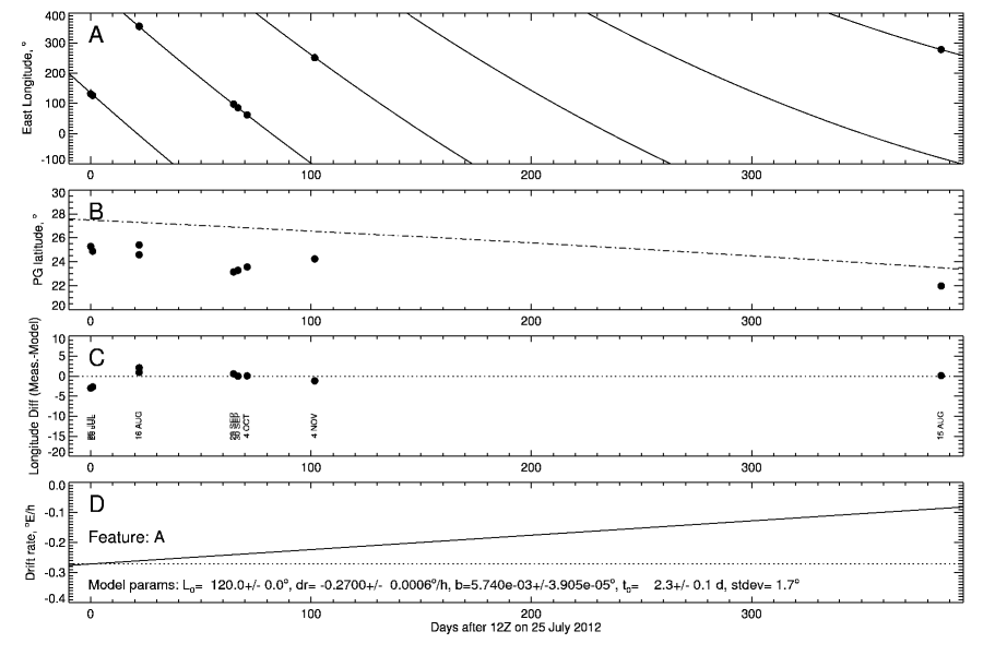
Figure 19.— (A): Longitude measurements for feature A (points) compared to a constant latitudinal drift model (solid line) (fit to Eq. 7). (B:) latitude measurements (points) compared to the latitudes (dot-dash line) computed by plugging fit coefficients $a$ and $b$ into Eq. 9, where $d\omega/d\theta$ was obtained from the S13A Model of drift rate versus latitude. This model is compatible with the observed latitudinal rate of change in (B), but not with the absolute value of the latitude, which the model exceeds by about 2^∘. (C) measured longitudes (points) minus model longitudes. (D) Drift rate versus time, inferred from fitting Eq. 7 to the longitude observations and then plugging the coefficients $a$ and $b$ into Eq. 8. The x coordinate in each panel is the time in days relative to 25 July 2012 at 12:00 UT.

Feature B had a nearly linear drift rate of -0.060^∘/h during 2012, and a drift rate of +0.0259^∘/h during 2013. This can be joined and well fit with a sinusoidal model, using an average drift rate of -0.0176^∘/h (-0.442^∘/day), an oscillation amplitude of 118^∘, a period of 686 days (shown in Fig. 20). This model is also consistent with the observed latitudinal drift over that time period (see panel B), but the model latitude is about 2^∘ S of the observed latitude, an offset opposite to that observed for A, but consistent with what is shown in image B2 of Fig. 17.

A feature seen in 2006 and either the same or another feature seen in 2007 (Sromovsky et al. 2012c) appeared at about 27^∘N, close to the latitude observed for features A and B. These earlier features also seemed to be associated with dark spots, and the 2006 feature was seen as a dark spot in an HST ACS image at 658 nm (Hammel et al. 2009). These might be related to either A or B in our current data set, based on similarity in morphology as well as latitude.

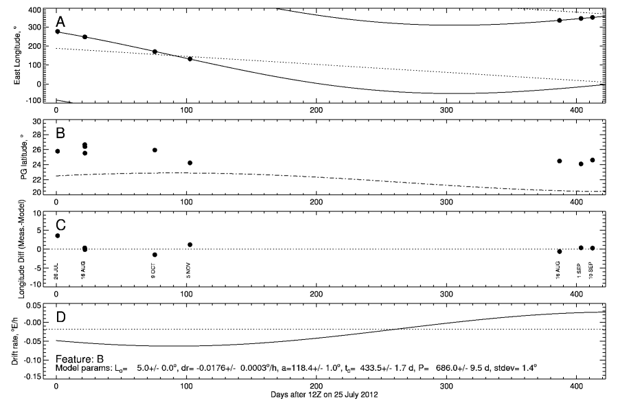
Figure 20.— As in Fig. 19, except that longitudes here are for feature B and the model is defined by Eqs. 10 - 12. This feature has a drift rate of -0.060^∘/h for the first 100 days (from July to November 2012) and 0.026^∘/h during August-September 2013. This variation is compatible with a sinusoidal variation in longitude, as shown in panel C, a sinusoidal variation in drift rate (D), and a sinusoidal variation in latitude, as shown by the dot-dash curve in B, where the latitudinal model is obtained from Eq. 12, which in this case shows a 2^∘ deficit relative to the observed latitudes (points).

5.2.2 Feature C

Feature C, located at about 36.5^∘ N, is the longest living feature we observed, appearing in August and November 2012 data sets, as well as in 2013 and 2014 data sets, including August as well as November 2014 images. It is also a feature that does not seem to have drifted in latitude over this time period, although its varying drift rate suggests a small oscillation in latitude of less than 1^∘ in amplitude. Feature C can also be roughly fit with model that includes a sinusoidal variation about a mean drift rate, with a much greater average drift rate of -1.2157^∘/h, compared to A or B, a much shorter period of variation (258 days) compared to B, and a much smaller amplitude of 27.5^∘ (see Fig. 21), which leads to a much smaller latitudinal variation (panel C) than feature B. However, the latitudinal measurements of C exhibit considerable scatter, especially in the latter 2014 observations, although for most of the range the observed and model latitudes are within 1-2 degrees, with the model being north of the measurements. A possible reason for the poorer fit of Feature C in comparison with features A and B is that C is near a latitude region containing many features that might perturb its motions, as well as being in a region of relatively high zonal wind shear, so that slight latitude shifts might yield significant changes in drift rate.

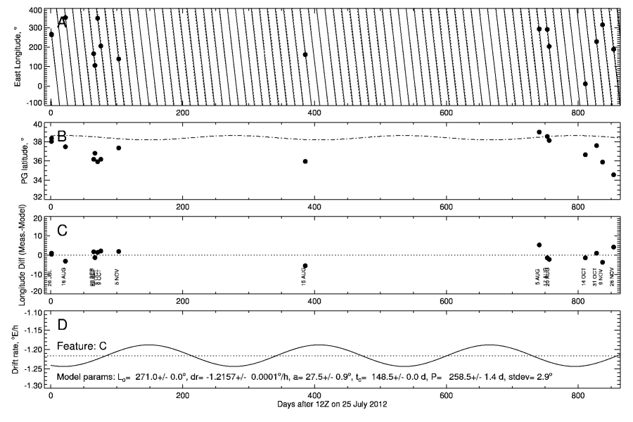
Figure 21.— As in Fig. 20, except that longitudes here are for feature C. This feature appears to have a relatively short period sinusoidal variation in longitude (A), relative to a baseline drift rate of -1.2157^∘/h, which implies a sinusoidal variation in drift rate (B), and a small sinusoidal variation in latitude (dot-dash curve in B), where the latitudinal model is obtained as in Fig. 20 and exceeds measured latitudes (points) by about 1^∘.

5.2.3 Features D and E

The southern hemisphere features D and E both were observed to move towards the equator during the two years spanned by our observations. And both appear to have existed for the entire time period, but are harder to observe because at their latitudes we can only see a small range of longitudes in any given image, a consequence of the sub-observer point being in the northern hemisphere. Feature D is relatively compact and is not difficult to measure when it can be seen. The longitude of feature E is particularly difficult to measure accurately because of the feature’s long narrow morphology.

Our model fit to D is displayed in Fig. 22. As it moves from about 35^∘ S to about 32^∘ S, its drift rate is seen to increase from -0.87^∘/h to -0.7^∘/h. The drift rate model, when converted to a latitudinal variation using Model S13A to relate drift rate to latitude, yields a latitudinal slope in good agreement with observations, and also agrees well with the absolute value of the latitude. A more accurate fit to the measured longitudes can be obtained with a baseline drift of -0.7145^∘/h, with drift rate varying from -0.73^∘/h to -0.52^∘/h, which reduces the RMS deviation from 14.1^∘ to 9.0^∘, but the inferred latitude then becomes about 3^∘ greater than the observed latitude. This might be a consequence of the cloud features being displaced in latitude from the circulation feature that is actually following the zonal mass flow. Both fits can be substantially improved by adding another component of variation, namely a sinusoidal deviation from the quadratic model, as shown by the dashed line in Fig. 22, which reduces the RMS deviation down to 1.9^∘ for the model that agrees well with the observed latitudes. That variation has a period of 750 days and an amplitude of 35^∘ in longitude. An even longer period of nearly three years was observed for a prior southern hemisphere long-lived feature named the Berg (Sromovsky et al. 2009). That feature spent most of its time oscillating $\pm$2^∘ about a mean latitude of 35.2^∘ S (planetographic), then in 2005 began to drift towards the equator, reaching 27^∘S by 2007 and reaching 5^∘S and dissipating in late 2009 (de Pater et al. 2011).

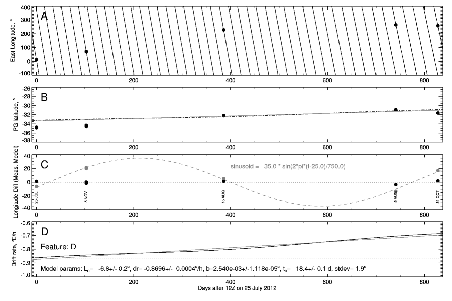
Figure 22.— As in Fig. 19, except that longitudes here are for feature D and the model is given by Eqs. 13 - 15. This feature appears to be drifting to the north and decreasing the magnitude of its negative drift rate in accord with the zonal wind profile. A model in which longitude relative to a baseline drift model (at -0.8695^∘/h) is assumed to vary as the square of a time difference provides a rougher fit that is compatible with a linearly varying drift rate (gray line in panel D) and a linearly varying latitude (gray line in panel B), where the latitudinal model is obtained as in Fig. 19, and in this case agrees as well with measured latitudes (points) as the more complete and accurate model (shown as solid black lines in A and D, dot-dash line in B, and dotted line in C). The additional sinusoidal variation contained in this model is shown by the dashed curve in panel C.

Feature E (model fit in Fig. 23) was first seen near 41^∘ S and last seen near 38^∘ S. Its latitude seems to follow a linear trend of about 1^∘/year towards the equator, and the longitudinal model fit is compatible with latitudinal variation obtained by interpolation of Model S13A of Sromovsky et al. (2012c). However, there are so few observations of this feature that we cannot entirely rule out other drift rate models.

All the features in the 2012-2014 data sets that were observed to have substantial latitudinal motions moved towards the equator, as did the previously mentioned Berg feature last seen in 2009.

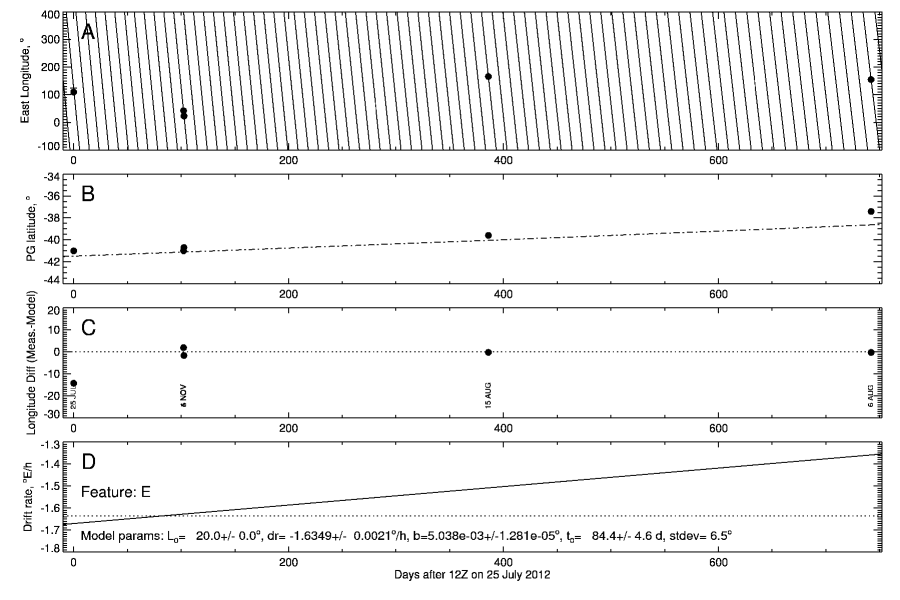
Figure 23.— As in Fig. 19, except that longitudes here are for feature E. This feature appears to be drifting in latitude and following the local wind profile. Observations of longitude (A) can be roughly fit with a constant drift rate, but the varying latitude (B) suggests a varying drift rate, and a fit to the difference from a constant drift rate using a quadratic function of time (C) provides a comparable fit that is also compatible with a linear latitudinal variation (B).

5.2.4 Feature F

Found near 34^∘N planetographic latitude (Figs. 16 and 17), feature F, which is feature 2 of de Pater et al. (2015), is the first discrete cloud feature ever clearly detected by amateurs using CCD detectors and small telescopes (de Pater et al. 2015). Compared to most other prominent northern-hemisphere features seen in 2014, feature F was not particularly bright at near-IR wavelengths and did not extend to as high an altitude. It was not seen in K^′ images, placing it deeper than the 1-bar level according to Fig. 3, while several other 2014 features were spectacularly bright at that wavelength, with G being the most notable (de Pater et al. 2015). Yet, it was F that was detected by amateurs, probably because it had a substantially greater optical depth than surrounding clouds. Feature F turned out to have an exceptionally long life and was tracked by amateurs as well as by HST observations using a ToO program 13712 (K. Sayanagi, PI) and OPAL program 13937 (A. Simon, PI), and by observations from Gemini, Keck, and Palomar, which are all summarized by Sayanagi and al. (2015). Our model fit to its motions is displayed in Fig. 24. We first saw F in our 2014 Keck images, but were not able to identify it in 2013 or 2012 images. This is not because of confusion about which feature is which. When we project our model backward we find no feature at all anywhere near the predicted location. Thus it appears that F developed sometime between August 2013 and August 2014.

F also has an unusual morphology. It appears to have a very short plume extending to the west on its north side and a very extensive plume extending eastward over more than 100^∘of longitude on its south side (see Figs. 16 and 17). The direction of the plume is consistent with cloud particles spreading out from F mainly to the south, then following the zonal flow and falling behind the faster (more westward) motion of F. Given the F-to-plume latitude distance of 3-4^∘ and the local wind shear of 0.084^∘/h per degree of latitude (from Table 6). The time to extend the plume 100^∘ of longitude would be 30 to 40 hours. Of course the length of the plume is also limited by particle fallout, so the time span of convective activity and plume generation could of course have been much longer. The prominence of the F plume is a marker of its unusual convective strength relative to other features in similar shear regions that generate no plumes and is consistent with a large optical depth that would facilitate amateur detection of the feature. The last observation of this feature at the time of this writing was obtained on 8 January 2015, using the Gemini NIRI imager. At that time it did not appear to have a prominent plume, suggesting that its convective activity has substantially declined. It was found just 12^∘ east of the location predicted using the model in Table 8.

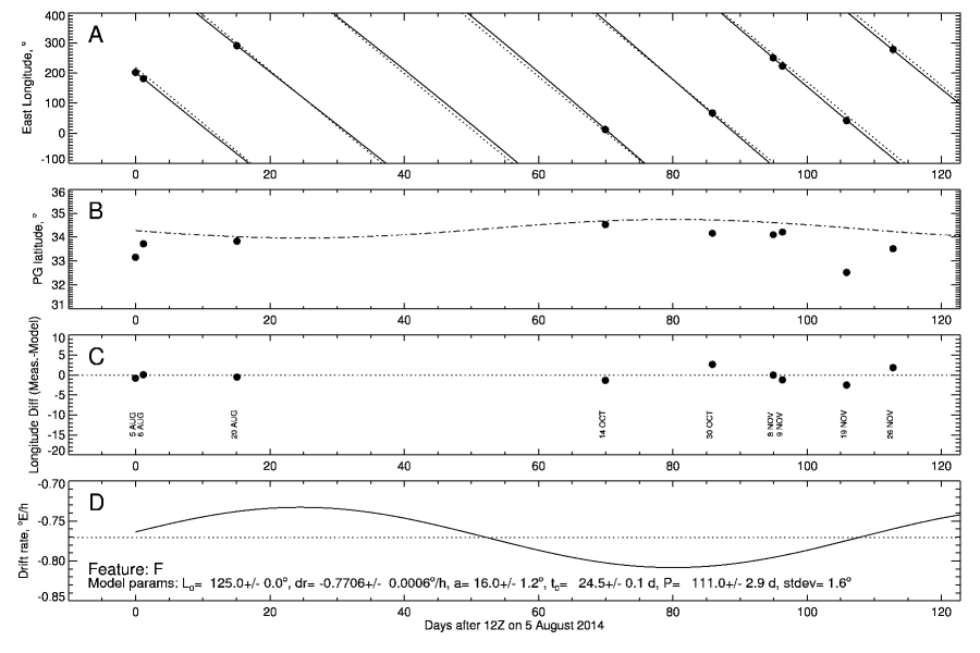
Figure 24.— As in Fig. 20, except that longitudes here are for feature F. This feature has a varying drift rate (solid lines in A and D), following a slow oscillation in longitude about a mean drift rate (dotted lines in A and D) of -0.7706$\pm$0.0006^∘/h, which is nearly consistent with the zonal flow at a mean latitude about 0.5^∘ north of the observed latitudes (filled dots in B). The latitudinal model shown as the dot-dash line in B is obtained as in Fig. 19.

5.3. Possible interactions of long-lived features

Long-lived features at nearby latitudes move at different longitudinal speeds and will eventually approach each other at close range, raising the possibility of some sort of interaction. An example of this occurred on 25 December 2011, when two bright features separated by 2^∘ in latitude had a close approach that resulted in formation of a small dark spot and companion clouds (Sromovsky et al. 2012a). A close approach observed on Saturn (Sromovsky et al. 1983) resulted in a more dramatic development of bright clouds during the interaction. It is also possible that features might merge or dissipate. Examples of dark spots merging on Saturn can be found in Fig. 3 of Porco et al. (2005). If the features have underlying vortex circulations of similar vorticities, we might expect to see latitudinal deflections in opposite directions as they pass by each other, followed by a return to their original latitudes. It is less clear what changes to expect in the structure of their companion clouds. We found no evidence of strong interactions for the two feature pairs described below.

5.3.1 Close approaches of A and B

Long-term tracking of A and B features show that B has an average drift rate of -0.0597$\pm$0.0002^∘/h, while A has an average drift rate of -0.248$\pm$0.002^∘/h, with this average taken over a period from late August 2012 to 4-5 November 2012. Given that the winds become more westward at higher latitudes, the drift rate comparison suggests that the putative vortex generating the A features is actually north of the vortex generating the B features. This is consistent with the November 4-5 appearance of the features in Fig. 17. The long term tracking of these two features, illustrated in Fig. 25, provides another surprising result. Since their sizes (judged by the extent of the bright clouds associated with them) are somewhat greater than the latitudinal difference between them, we would expect some sort of interaction when they pass by each other. However, even though they reached the same longitude on September 7, 2012, their drift rates before and after that close encounter were not perceptibly changed.

Features A and B had three more close encounters before our next observing run on 15-16 August 2013, yet they remained distinguishable features. However, there is considerable ambiguity as to what happened during the nearly 10 months without any observations. Extending the drift track of these features to the August 2013 date, we find close approaches should have occurred on 5 December 2012 and 25 March 2013. It is plausible that the multiple close approaches altered their latitudes and drift rates slightly, and our assumed model of a linear variation in latitude (and in drift rate) may not be correct. A non-uniformly varying drift rate has been observed for other long lived features on Uranus, so this would not be surprising. It is also possible that one or both of the features disappeared during that unobserved period and that at least one of them in our 2013 images is a new feature.

Also noteworthy, is that the latitudes we infer from our drift rate models interpolated to latitudes using the zonal profile of Sromovsky et al. (2012c), suggest that Feature A is following a circulation feature that is about 2^∘ N of the observed bright clouds and that Feature B is following a circulation feature this is about 3^∘ S of the bright clouds associated with it. In this connection it is worth noting that the rectangular projections of A2 and B2 in Fig. 17 for November 2012 (2nd row from bottom) provide evidence of a dark spot associated with A that is north of the bright clouds accompanying it, and a dark spot associated with B that is south of the bright clouds accompanying it. The inferred separation of about 5^∘ in latitude makes it somewhat more plausible that the features seem to suffer no major interactions.

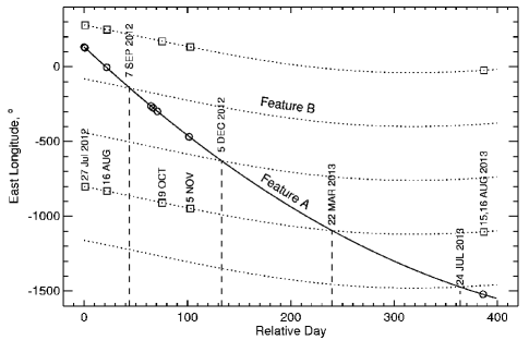
Figure 25.— Comparison of long term tracking results for features A and B. The x axis shows time in days relative to 25 July 2012 at 13:32:39 UT. The models of longitude versus time are those given in Figs. 19 and 20, the latter plotted with multiple 360^∘ offsets to show crossing events more clearly (these are marked by vertical dashed lines and annotated by date at which they reach the same longitude).

5.3.2 Close approaches of C and F

Close approaches of features C and F are shown by intersections of longitude versus time plots in Fig. 26. The average latitudes for Features C and F are 36^∘ N and 34^∘ N respectively. Since each of these appears to extend over several degrees of latitude (see Fig. 17), it would be surprising if they did not display evidence of some interaction. In fact, these were observed in such close proximity in HST images acquired on 14 October 2014 (taken as part of a Target of Opportunity program, with Kunio Sayanagi as PI), that we initially thought we were observing a single feature. We also observed them in close proximity in a Gemini NIRI image acquired on 19 November, about 1 day after close approach. Both of these close approaches are consistent with the longitude versus time plots shown in Fig.  26. Besides the 14 October and 18 November approaches, we also found unobserved close approaches on 12 September 2014 and 20 December 2014. There is no evidence of any change in drift rate or, based on a 26 November Gemini image, any change in the morphology of the features following these possible interactions, although F was seen close to the central meridian only in the late November image.

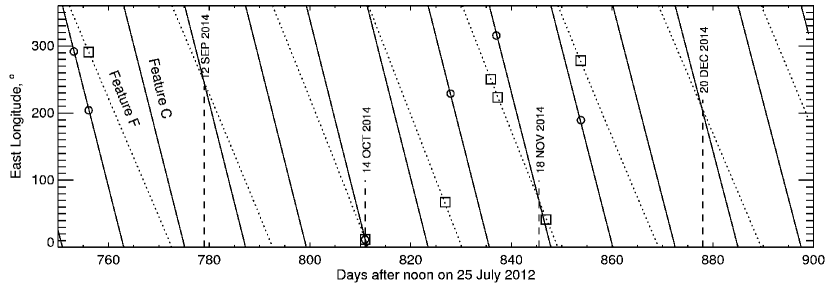
Figure 26.— Comparison of long term tracking results for features C and F. The x axis shows time in days relative to 25 July 2012 at 12:00 UT. The models of longitude versus time are those given in Figs. 19 and 20, each plotted with multiple 360^∘ offsets to show crossing events (these are marked by vertical dashed lines and annotated by date at which they reach the same longitude). Measured points are plotted as circles (for feature C) and squares (for F). Note the overlap of measurements on 14 October 2014.

5.4. Unusually bright feature G

de Pater et al. (2015) identified several bright features in the 2014 Keck observations, one of exceptional brightness, which is labeled as G in Fig. 16. This appears to have faded dramatically within a month or so. A similarly bright cloud feature was detected in August 2005 (Sromovsky et al. 2007), but at a higher latitude (31^∘N). It brightened and faded dramatically within a few months, and extended to similarly high altitudes ($\sim$300 mbar level).

6. High latitude polar cloud features.

6.1. Feature morphology

The 2007 equinox observations (Sromovsky et al. 2009) provided the first detection of cloud features north of the 60^∘N westward jet peak. More features were seen in 2011 images, and it appeared that the north polar region was peppered with small low-contrast discrete clouds Sromovsky et al. (2012c), presenting what looked like a field of fair-weather cumulus convection on earth, but on a much larger scale. This was not expected because such features had never been seen in the south polar region. From 2012 onward, the improved views of the north polar region of Uranus have allowed us to combine observations from successive observing nights to form a complete picture of the polar region. Because the entire region from about 63^∘N to at least 83^∘N moves in solid body rotation, we were able to average images with that rotation period removed to obtain a pole-centered high S/N view of Uranus’ north polar region for each of the three years of observation (Fig. 27). These show a continued prevalence of large numbers of small bright features.

Almost all the polar bright features have similar size and shape, which is mainly circular. Typical diameters are 600-800 km, which is comparable to imaging resolution, and thus is an upper limit for the smaller features. There are also less numerous but well-defined small dark spots, many of which are well separated from bright spots and thus cannot be explained as an artifact of high-pass filtering. The small bright features have a typical contrast of 1-2% in the raw images, with a much brighter than typical feature in the 4-5 November image reaching 10%. The dark features have only a fraction of the contrast of the bright features (as well as the opposite sign). The lifetimes of the polar features can extend for at least 1.5 planet rotations, as quite a few of these have been tracked over that time period (not continuously, but with a one- rotation gap). The large number of features seen in the November 2012 data set seems to indicate the clear peak in activity. At a casual glance these spots appear to be fairly uniformly distributed in latitude and longitude, down to a latitude of about 55^∘N, where there begins a transition to a morphology dominated by longitudinally stretched streaky features often occurring within long narrow regions of enhanced brightness with a width comparable to the diameter of the small polar spots. However, there is a pattern in the distribution of features that has at least some crude year-to-year consistency, as discussed in Section 6.2.

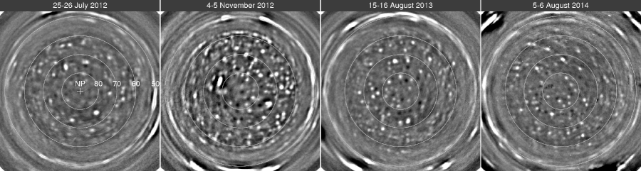
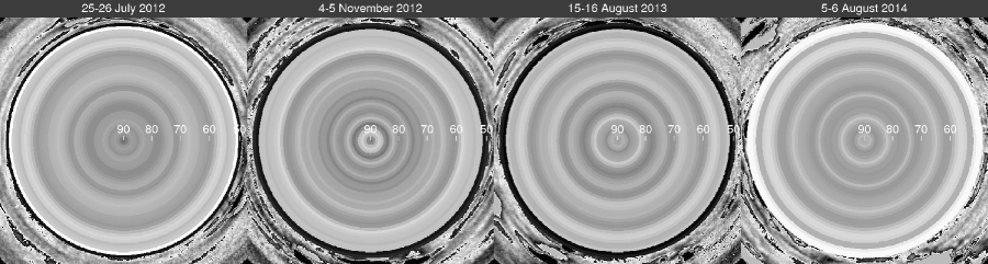
Figure 27.— Polar composites (top row) from 2012, 2013, and 2014, in which images were averaged after removing a fixed 4.1^∘/h rotation relative to the planet’s fixed coordinate system. The lack of zonal smearing at latitudes greater than 55^∘N confirm the existence of precise solid body rotation in this region. These images were high-pass filtered with a smoothing length of 25 pixels, compared to a displayed image size of 500 pixels. Zonal averages of the composites in 1^∘ bins (bottom row), showing a crudely consistent pattern in the location of bright features.

It is worth recalling, as demonstrated in Fig. 1 of Sromovsky et al. (2014), that when the south polar region was imaged in 2003, using the same telescope, camera, and essentially similar AO system, no discrete polar features of any kind were observed between 50^∘S and the south pole. That observation was made in southern hemisphere fall, while the current observations were made during northern hemisphere spring. One might surmise that this seasonal difference is the cause of this striking morphological asymmetry. A long season of radiative cooling from the top of the atmosphere during Uranus’ northern winter might tend to produce an unstable thermal profile that favors vertical mixing, which is likely to be most active following equinox. On the other hand, the long summer of heating from above during southern hemisphere summer might stabilize the thermal profile and inhibit vertical convection in southern polar regions in the fall. Although this has a plausible ring to it, there are other indicators of vertical convection, such as depleted methane mixing ratios in both polar regions at the same time (Sromovsky et al. 2014), which argues against such seasonal modulations in at least the large scale flow. We are expecting that this “convective” activity might continue for a while as the northern hemisphere moves into summer, but it is plausible to expect it to eventually dissipate as summer heating intensifies. We also expect the formation of a polar cap cloud (Hammel and Lockwood 2007), which appears to have begun (de Pater et al. 2015).

6.2. Zonal-average patterns in polar clouds

A closer look reveals that the zonal average relative brightness between 50^∘N and 90^∘N displays a roughly consistent pattern, evident in the zonally averaged polar projections in Fig. 27, and the plot of relative brightness versus latitude in Fig. 28. In the average for all three years, the two 2012 values are averaged together to represent the average for that year. All three years have minima near planetographic latitudes of 53-54^∘N, 60-61^∘N, 70-71^∘N, and 76-80^∘N, though the 2012 November 4-5 composite is somewhat of an anomaly, with both larger numbers of polar features and features of greater contrast than seen in other years. Other details regarding positioning and widths and numbers of various bands vary from year to year. Between 60^∘N and 80^∘N, the August 2012 and 2013 composites have better pattern agreement with each other than either has with the 2014 composite. But at 80^∘ N and 90^∘ N the 2013 and 2014 composites agree much better with each other than with the 2012 composites. Whether these changes from year to year are real trends, or just due to stochastic variations is hard to evaluate without more observations. Certainly 2012 demonstrates considerable variability within a single year. The 3-year average pattern is roughly consistent with observed high-latitude variations in the apparent methane mixing ratio inferred from 2012 STIS observations by Sromovsky et al. (2014), who noted the correlation with 2012 Keck observations. They also pointed out that these apparent mixing ratio variations might actually be caused by para fraction variations induced by local vertical convection.

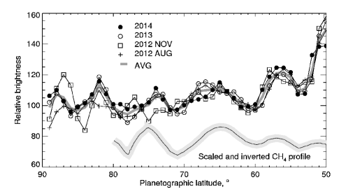
Figure 28.— Zonal average of relative brightness as a function of latitude for each data set during 2012-2014 (thin lines), derived from polar composites displayed in Fig. 27. The average over all data sets (giving equal weights to each year) is plotted as a thick dark gray curve, and a scaled and inverted version of the methane profile of Sromovsky et al. (2014) is plotted in the lower part of the figure, where the variations between 60^∘ and 80^∘ correspond to CH₄ volume mixing ratio variations of about $\pm$0.005 relative to a mean of 0.02. As noted by Sromovsky et al. (2014), these variation might actually be caused by para fraction variations induced by local vertical convection.

A more detailed view of polar cloud features is presented in Fig. 29, where we see that almost all features have about the same size, which is 600 km to 800 km according to 2-D Gaussian fits to many of the features. Line scans through several bright and dark spots are plotted in the bottom panel of Fig. 29, showing that both bright and dark features have FWHM values comparable to the Keck NIRC2 PSF (about 0.06^′′). Thus, these features are generally not resolved and might actually be considerably smaller than they appear in these images. The dark spots, which are possibly regions of reduced cloud opacity, perhaps produced by downwelling motions, have lower contrast than bright features, but are of similar apparent size. Spacing between features is typically 1000 km to several thousand km. The dark spots are generally found at higher latitudes than the bright features, most within 20^∘ of the pole. There is also another change in distribution between regions close to the pole, where spots appear to be randomly distributed, and regions further from the pole, where features seem to appear more often as beads on a string, with the “string” in this case lying along a circle of constant latitude.

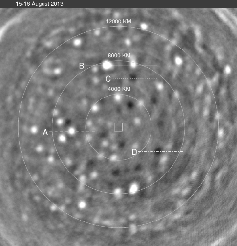
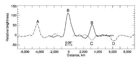
Figure 29.— Detailed view of polar bright and dark spots in August 2013 (upper) and line scans through several spot features (lower). Note that dark spots often occur in isolation from bright features. Line scans indicate that the spot features are generally not resolved; they appear to have Gaussian cross sections and full-width-half-maximum values comparable to that of the imaging system (about 0.06^′′ in H under ideal conditions). In the upper panel, circles of constant distances from the pole provide a sense of the physical scale. The small square centered at the pole is 1000 km on a side. This image was also high-pass filtered as in Fig. 27. The contrast in unfiltered images was measured to be 2.7% for the brighter feature along scan B and 2% for the feature intersected by scan A.

7. Near-equatorial waves

One of the more striking features in Uranus’ atmosphere is the scalloped wave form that was first brought to light by high-S/N measurements in 2012. The immediate appearance is that of two sine waves that criss-cross each other, similar to a two strand braid (Fiq. 18). This appears strikingly similar to vertically varying cloud forms created by Kelvin-Helmholtz instabilities generated by sharp vertical gradients in the horizontal winds. A different wave mechanism must be at work here however, perhaps Kelvin waves or mixed internal gravity-Rossby waves. A correct identification would be helped by measuring its dispersion relation (phase speed versus wavelength), which is not likely to be feasible with current observations. The lower boundary of this morphology is a sort of ribbon wave (Fiq. 30), though the ribbon does not have a constant latitudinal width. The better defined upper boundary of the ribbon, which is the lower boundary of the scalloped features, is somewhat sinusoidal, with a longitudinal wavelength of about 20^∘ (corresponding to a wavenumber of 17 to 19), with only a small decrease from 21^∘ in 2012 to 19^∘ in 2014, and a latitudinal peak-to-peak amplitude of about 2.4-2.9^∘. The dark ribbon itself has a width of about 1-2^∘ in latitude. The ribbon continues around the planet, but the transverse wave does not; instead it seems highly damped on one side and well defined on the other. This can be seen from images in Fig. 2, specifically pairs taken on successive nights, which look at opposite sides of the planet. For example, compare pairs B-D, J-L, N-P, and R-T. In the last case, instead of the transverse wave, we see small discrete bright features in the same latitude region. These characteristics are more clearly evident in the rectangular maps of Fig. 16, especially in the 2012 maps.

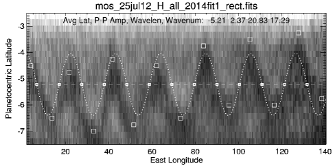
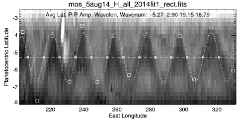
Figure 30.— South-equatorial waves in 2012 (top) and 2014 (bottom), with sinusoidal fits for each to the lower boundary of the bright region above the dark “ribbon” feature. For context, see Fig. 2.

Ribbon waves have also been seen in the cloud forms on Saturn, one located at the peak of a mid-latitude eastward jet in the northern hemisphere (Sromovsky et al. 1983) and one located near the peak of an eastward jet in the southern hemisphere (Sanchez-Lavega et al. 2000). The latter waves had peak-to-peak amplitudes of 1-1.3^∘ in latitude, and wavelengths of 5-6^∘ in longitude, smaller than the waves we observed on Uranus by a factor of two in amplitude and a factor of four in wavelength. The mechanism suggested to explain the Saturnian waves is baroclinic instability (Godfrey and Moore 1986). A viable mechanism that might explain the uranian ribbon wave remains to be determined.

8. Persistent latitudinal patterns in reflectivity

To investigate the latitudinal band patterns over the whole globe we sampled our mosaicked images in narrow latitude bands, computing both zonal means and zonal median values to avoid the contributions of bright cloud features. The results from each time period are shown in Fig. 31 in image form and in Fig. 32 as normalized plots. The zonal average, shown in the top panel in Fig. 31 includes the effect of discrete cloud features, and the bright bands in the 2014 image are due to the eruption in cloud activity during that year. The median images (lower panel) are much less affected by discrete cloud features and yet show many of the same persistent patterns, especially the brighter bands near 40-50^∘S, 10-20^∘S, 0-8^∘N, 10-12^∘N, 18-31^∘N, 38-42^∘N, and 48-52^∘N. The exceptions are mainly for the 2014 observations where the large number of discrete features has apparently obscured the background band patterns in the northern hemisphere. The plots of latitudinal profiles in Fig. 32 make clear how subtle the patterns really are. These features cannot be directly discerned in the direct averages and median profiles shown in panel A. They only become obvious when the profiles have their smoothed versions subtracted, and the difference amplified by a factor of 100, as in panels B and C.

The large scale relative changes in panel A with latitude are somewhat distorted by the variation of effective view angle with latitude in the mosaicked images, especially at high southern latitudes, where the effective view angle cosines are of necessity much smaller than for mid-latitudes and for all of the northern hemisphere. To examine this issue we formed a median image without remapping to a fixed time, then sampled latitudinal brightness profiles at fixed view angle cosines. At $\mu=0.3$ we found that in July 2012 the I/F at 50^∘ N was about 25% brighter than the equator when compared at the same view angles, but 18% brighter in the mosaicked images. The same comparison at 45^∘S, found a ratio of 0.95 for the sampling at equal view angles, but 0.83 in our mosaicked image. However, the trend of increasing brightness with time at high northern latitudes is also seen when sampled at constant view angle, as is the trend of darkening with time at high southern latitudes, both with respect to equatorial values.

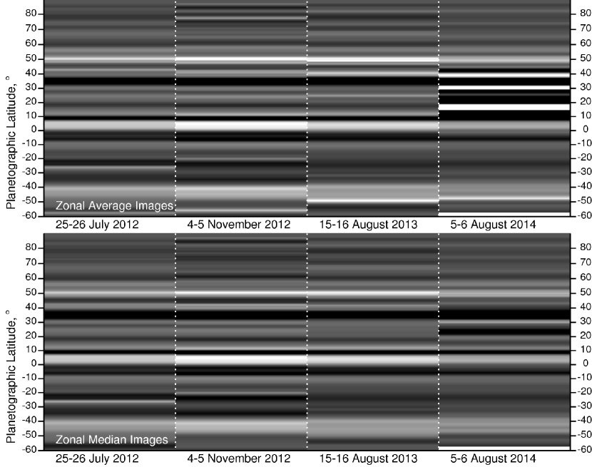
Figure 31.— Images of zonal mean (top) and zonal median (bottom) relative brightness values obtained from high-pass filtered mosaicked image maps displayed in Fig. 16. The median images avoid contributions from discrete cloud features. In both images black and white correspond to approximate I/F deviations of -0.4$\times 10^{-4}$ and +0.8$\times 10^{-4}$ respectively (the central disk I/F in H is about 0.01).

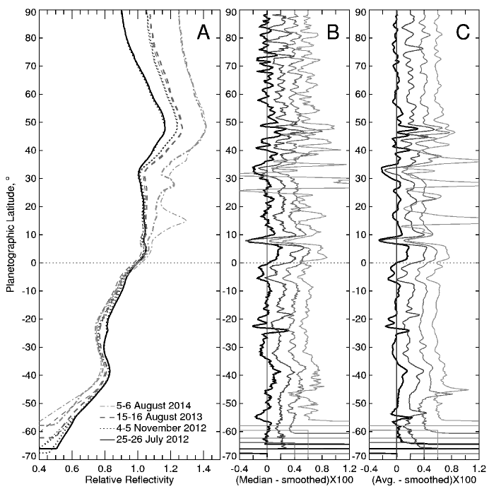
Figure 32.— Zonal mean and zonal median reflectivities from rectangular maps of mosaicked images without high pass filtering and normalized to 1.0 at the equator (A), and high-pass filtered deviation profiles for median (B), and mean (C) values for each data set. The subtracted smooth profiles used a 3.25^∘ boxcar. In A, thinner lines show mean brightness (which includes discrete cloud contribution) and thicker lines show median brightness. In B and C the lightest curve is for the earliest data set (25-26 July, 2012) and the darkest curve is for the latest.

9. Cloud composition and vertical structure

9.1. Cloud composition

The composition of the clouds is constrained by indirect measurements. Spectral observations show that the main condensable in the upper troposphere is methane. At the pressures and temperatures of the brighter clouds (about 1 bar and 77 Kelvin) it seems certain that they are mainly made of frozen methane particles. The deeper clouds, at pressures near 1.6 bars, are less certain. H₂S is a good candidate for these clouds, along with NH₄SH for the even deeper layers (de Pater et al. 1991).

9.2. Vertical structure

The spectral filters used in our high-S/N observing program had to be very limited due to the time required to obtain high S/N ratios. Besides our primary H filter, we also used Hcont, CH4S, and limited K^′ filters, to provide constraints on effective cloud altitudes (see Fig. 3), although we cannot constrain the many parameters of a detailed vertical structure model with these observations. Effective altitudes were estimated for major features seen in 2014 images by de Pater et al. (2015), finding that the larger bright feature had effective cloud top pressures from as low as 300 mb to as high as 1.2 bars. From a similar analysis of northern high-latitude features in 2011 Keck images, Sromovsky et al. (2012c) found cloud altitudes of 200 mb to 400 mb for the two brightest features, and found that the small polar cloud features (many unresolved) were at considerably higher pressures, most in the 1-2 bar range. Since the latter analysis, it has been confirmed that the methane mixing ratio at high polar latitudes is depleted substantially in the upper troposphere relative to low latitudes (Sromovsky et al. 2014). That implies that a more complex analysis is needed to interpret spectral constraints on cloud altitudes in the north polar region, which we leave for future work. For the moment, we can provide a qualitative view of relative cloud height differences using H and Hcont images from our 2012 Keck data set. In Fig. 33, we display two color-composite images in which we assign Hcont to blue and green color channels, and H to the red color channel. Deep clouds are attenuated more in H than in Hcont, so they appear to have a blue tint, while higher altitude clouds of low optical depth have relatively greater brightness increases above background in H than in Hcont, thus appearing with a red tint, while optically thick high altitude clouds can appear equally bright in both channels, and thus can appear white, with appropriate display enhancements.

Among the high-altitude features, based on their visibility in K^′ images, we find that B and C reached pressures less than one bar. No features reached that level in the southern hemisphere. We suspect that feature A may have reached that level in 2012, but lacking any K^′ images from that period, we need to carry out a full radiative transfer analysis to confirm it. Its bright clouds were not visible in K^′ images from 2013 and 2014. Feature F was the only feature prominent in amateur images from 2014, which were typically taken with a 625-nm long-pass filter (cut off by CCD response falloff). F is not a high-altitude feature; it is not visible in Keck K^′ images, but apparently is of sufficient optical thickness to provide contrast at wavelengths with less methane absorption. At these wavelengths, the background atmosphere becomes too bright to allow detection of optically thin high-altitude features, even though they can be very prominent in K^′ images. An analysis of cloud pressures for major 2014 features by (de Pater et al. 2015) shows that C4 (their feature 1) reached levels of 420-720 mbar, that F (their feature 2) did not extend much above 2 bars, while G (their feature Br) had a complex structure with component elements reaching pressures from 300-700 mbar.

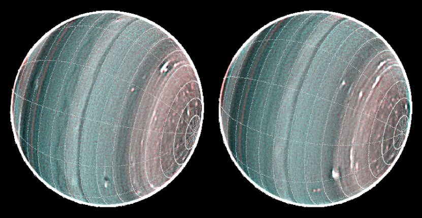
Figure 33.— Broad cloud altitude changes indicated by H and Hcont brightness differences in these 25 (L) and 26 (R) July 2012 image composites. Here low altitude clouds have a blue tint, high altitude optically thin clouds have a red tint, while clouds that are both high and optically thick appear white. Some of the color gradient between high and low latitudes may be related to the decline in the upper tropospheric methane mixing ratio with latitude. These images have been processed to amplify the high spatial frequencies using I(enhanced)=I + k*(I-smoothed(I)), with k set to 35 and the smoothing length set to 9 pixels (0.09 arcseconds). The grid intervals are 10^∘ in planetographic latitude and 30^∘ in longitude.

10. Discussion: Polar circulation and static stability

There may be a connection between the numerous small, apparently convective, cloud features in the north polar region of Uranus, and its circulation being solid-body over the region where this suggested convection occurs. If the static stability (as measured by its Brunt-Vaisala frequency or its Rossby deformation radius $L_{R}$ (Pedlosky 1982)) were large, then the planetary east-west flow would be expected to act as if were two-dimensional and quasi-geostrophic (QG) (Marcus 1993). In the mid-latitudes between 10^∘ and 60^∘ in both hemispheres, we can show that the mean east-west flow is well-approximated with a QG model with an $L_{R}\simeq 6000$ km and with a weak potential vorticity gradient, in accord with Deng and LeBeau (2007). A QG model does not approximate the flow well in the region of the equatorial jet, where the Coriolis parameter passes through zero and where the east-west flow is likely to be more three-dimensional and driven by cellular motions such as a Hadley cell (Yamazaki et al. 2005). In addition, a QG model does not approximate the near solid-body rotation that we observe at the north polar region of Uranus. On the other hand, if the north polar region has low static stability with intermittent, local convection and/or baroclinic instabilities, as suggested by the region’s profuse clouds and by the fact that it recently passed from winter to summer (see Section 6.1), then there is reason to expect that solid-body rotation would develop there.

In modeling stars, it was traditionally believed that the turbulent mixing within convection zones made the convective regions of stars rotate as solid bodies (Maeder and Meynet 2000). In fact, a number of different authors have argued that in convectively stable regions of stars with internal gravity waves or with baroclinic instabilities, such as the Goldreich-Schubert-Fricke instability, the flow is driven to solid-body rotation (Maeder and Meynet 2000). However, measurements of the rotation curves in our sun, using helioseismology (c.f., Fig. 5 in (Beck 2000)) show a more complex picture of rotation. Solar observations, along with three-dimensional numerical simulations (Miesch et al. 2006) in which there is mixing, show that only polar regions within 20^∘ – 30^∘ of the poles rotate as solid bodies. Although there is differential rotation in the outermost surface of the sun, deeper, at the boundary of the convection zone and the radiative region (which is a nearly spherical surface with constant pressure), there is near solid-body rotation. (See the comparison between the surfaces of constant rotation and the location of the convective zone boundary in Fig. 1 of Balbus et al. (2009)). Because we expect that clouds that we use in determining the east-west velocities or Uranus are located near the boundary of its convective and radiative zones, it is the differential (or lack thereof) rotation curve at this boundary that is relevant to us.

A simple argument by Balbus (2009) based on weak instability and the thermal wind equation explains the solid-body rotation at the poles and differential rotation elsewhere. His original argument required that the weak instability be due to magnetic fields, but later showed that any weak instability, including convective or baroclinic, would suffice (Balbus et al. 2009). The decrease in the static stability at the north pole of Uranus due to the cooling of the atmosphere during winter over the long season of darkness may be sufficient to allow weak, new baroclinic instabilities to form or old instabilities to strengthen and cause the north polar region to rotate as a solid body during its winter and spring. If this connection between solid body rotation and weak static stability is valid, then as the north polar region of Uranus passes into summer, we would expect to observe a decrease in the number of clouds at the north polar region and an increase in its differential rotation. Future observations should be capable of testing this hypothesis.

The angular velocity acceleration needed to transform the polar circulation from the solid body form seen in north polar spring to the more complex form seen at southern hemisphere solstice might be produced by vertical advection of angular momentum from below or from poleward meridional motions, for which conservation of angular momentum would tend to increase angular velocity with decreasing distance to the pole. Whether such a transformation actually takes place, and how effective these mechanisms might be in producing the speculated transformation remains to be determined.

11. Summary and Conclusions

We reported on the analysis of an extensive data set of high-quality AO images acquired from Keck and Gemini observatories from 2012 through 2014. Further enhancement of image quality was obtained by averaging multiple images in a body fixed coordinate system, allowing the improvement of signal to noise ratios while avoiding the smear due to planet rotation. Our results are summarized below.

1. We made over 850 measurements of cloud features in high-S/N images from 2012, 2013, and 2014. These are heavily weighted towards the northern hemisphere not only because the sub-earth and sub-solar latitudes were in the northern hemisphere, but also because Uranus produced more cloud features there. The number of trackable cloud features in 2014 was exceptionally large compared to other years. Gemini observations produced far fewer trackable features than Keck observations, mainly due to the higher performance of the Keck AO system as a result of its ability to use Uranus as a wave-front reference.

2. These observations revealed an active polar region, with many small cloud features of 600-800 km, comparable to the Keck telescope’s resolution. Most of the features are bright, but a number of dark features were also seen of about the same size and mainly circular shape. These features are found between the north pole and about 55^∘N. The small polar cloud features were seen in every year of high-S/N observations, but were most apparent in 4-5 November 2012 observations, where they seemed to have higher contrast and greater numbers. A sizable fraction of these features lived long enough to track on successive nights, providing an accurate determination of their wind speeds.

3. Our new measurements firmly established that the high-latitude zonal winds of Uranus, between 60^∘N and at least 83^∘N, closely adhere to solid-body rotation at a rate of 4.08$\pm$0.015^∘/h westward relative to body-fixed coordinates. When winds are plotted in units of m/s, the transition to solid-body rotation appears as a zonal jet with a peak velocity of 260 m/s westward

4. We were able to fill in details of the zonal profile in the 12^∘N - 30^∘N region, which has been under-sampled in prior data sets.

5. Binned wind measurements show a stair-step appearance at middle latitudes, suggesting that the wind profile may not be an entirely smooth function of latitude.

6. We discovered a substantial difference between the near-equatorial motions of waves and those of small discrete cloud features, with the former moving at a speed of 0.4^∘/h eastward and the latter at a speed of 0.1^∘/h eastward. This may mean that the equatorial mass flow is much slower than previously inferred and that the waves move eastward faster than the zonal flow by 0.3^∘/h.

7. Three symmetric (even order) Legendre polynomial fits were derived from the new wind observations. One is based on essentially the entire data set. A second is based on observations including the wave motions but excluding the small discrete feature tracking that was obtained from the 2014 observations, and a third is based on observations that exclude the wave motion measurements.

8. We also found that the preponderance of current and past observations are consistent with a north-south mid-latitude asymmetry in the zonal wind profile of Uranus. Using an asymmetric model to characterize this difference, we find that the maximum asymmetry amplitude is 0.09^∘/h when all high accuracy observations from Voyager onward are included, and 0.135^∘/h, when all but 2012-2104 observations are included, with the main asymmetries peaking near $\pm$30^∘. It appears that the asymmetry has decreased with time. We did not include in this analysis the enormous high-latitude asymmetry implied by the recent reanalysis of Voyager images by Karkoschka (2015).

9. Although there are no HST or groundbased wind measurements at high southern latitudes (50^∘S - 90^∘S), a recent reanalysis of 1986 Voyager 2 Uranus observations by Karkoschka (2015) has yielded wind results there that are very different from northern winds at corresponding northern latitudes. This large north-south asymmetry might be seasonal. However, only minimal changes have been seen in the north polar region between 2011 and 2014, and at middle latitudes only tiny changes have been seen since 1986. This argues against a large seasonal change in polar winds, though it cannot be ruled out.

10. We found two types of equatorial wave features. One type, seen in prior observations, as well as in our more recent observations, are diffuse bright features a few degrees north of the equator, spaced about 30^∘ to 40^∘ apart in longitude. The other kind of wave feature, not observed prior to these high S/N observations, is a transverse wave marked by a dark ribbon with a latitudinal width of about 1^∘ and a longitudinal wavelength of about 20^∘. However, the transverse wave amplitude, which is of the order of several degrees of latitude over about half of the planet’s circumference, damps to nearly zero over the remaining longitude range.

11. We found that zonal averages of brightness of polar cloud features has a latitudinal pattern in which brightness minima occur near 53.5^∘N, 61^∘N, 71.5^∘N, and 78^∘N. This is a good match to the apparent CH₄ mixing ratio variations inferred by Sromovsky et al. (2014). More obvious patterns are seen at lower latitudes, but most are only visible with high-pass filtering.

12. Zonal maps made from images acquired on successive nights in August 2012, November 2012, August 2013, and August 2014, show persistent patterns, and six easily distinguished long-lived cloud features, which we were able to track for long periods that ranged from 5 months to over two years. Two at similar latitudes are associated with dark spots, and move with the atmospheric zonal flow close to the location of their associated dark spot instead of following the flow at the latitude of the bright features. These features retained their morphologies and drift rates in spite of several close interactions. A second pair of features at similar latitudes also survived several close approaches. Several of the long-lived features also exhibited equatorward drifts and latitudinal oscillations.

13. Among the high-altitude features, based on their visibility in K^′ images, we find that B and C reached pressures less than one bar, and thus are likely at least partly composed of methane ice. No features reached that level in the southern hemisphere. We suspect that Feature A reached that level in 2012, but lacking any K^′ images from that period we would need a full radiative transfer analysis to confirm it.

14. There is a correlation between the region of polar “convective” cloud forms and the region of solid body rotation, both extending from about 60^∘ N to at least 83^∘ N. There are dynamical reasons to expect that these might be related, and that when the convection subsides, the winds might also change.

As Uranus moves towards its 2030 northern hemisphere summer solstice, a large seasonal shift in wind speeds should occur if the recent results of Karkoschka (2015) for the southern hemisphere indicate a seasonal asymmetry. What also might happen is that the cloud features that we currently use to track motions in this region either disappear or become obscured by an overlying haze, a result suggested by the fact that we have never seen near-IR cloud features in the south polar region. We can only hope that any seasonal changes will become observable before the tracers we use to observe them disappear.

References

- Alexander (1965) Alexander, A. F. O., 1965. The planet Uranus; a history of observation, theory, and discovery. New York, American Elsevier Pub. Co., 1965.
- Allison et al. (1991) Allison, M., Beebe, R. F., Conrath, B. J., Hinson, D. P., Ingersoll, A. P., 1991. Uranus atmospheric dynamics and circulation. In: Bergstralh, J. T., Miner, E. D., Matthews, M. S. (Eds.), Uranus. University of Arizona, Tucson, pp. 253–295.
- Archinal et al. (2011) Archinal, B. A., AHearn, M. F., Bowell, E., Conrad, A., Consolmagno, G. J., Courtin, R., Fukushima, T., Hestroffer, D., Hilton, J. L., Krasinsky, G. A., Neumann, G., Oberst, J., Seidelmann, P. K., Stooke, P., Tholen, D. J., Thomas, P. C., Williams, I. P., 2011. Report of the IAU Working Group on Cartographic Coordinates and Rotational Elements: 2009. Cel. Mech. & Dyn. Astr. 109, 101–135.
- Balbus (2009) Balbus, S. A., 2009. A simple model for solar isorotational contours. Monthly Notices of the Royal Astronomical Society 395 (4), 2056–2064.
- Balbus et al. (2009) Balbus, S. A., Bonart, J., Latter, H. N., Weiss, N. O., 2009. Differential rotation and convection in the sun. Monthly Notices of the Royal Astronomical Society 400 (1), 176–182.
- Beck (2000) Beck, J. G., 2000. A comparison of differential rotation measurements–(invited review). Solar Physics 191 (1), 47–70.
- de Pater et al. (1991) de Pater, I., Romani, P. N., Atreya, S. K., 1991. Possible microwave absorption by H2S gas in Uranus’ and Neptune’s atmospheres. Icarus 91, 220–233.
- de Pater et al. (2011) de Pater, I., Sromovsky, L., Hammel, H. B., Fry, P. M., LeBeau, R. P., Rages, K. A., Showalter, M. R., Matthews, K., 2011. Post-equinox Observations of Uranus: Berg’s Evolution, vertical structure, and track towards the equator. Icarus 215, 332–345.
- de Pater et al. (2015) de Pater, I., Sromovsky, L. A., Fry, P. M., , Hammel, H. B., Baranec, C., Sayanagi, K., 2015. Record-breaking storm activity on Uranus in 2014. Icarus 252, 121–128.
- Deng and LeBeau (2007) Deng, X., LeBeau, R. P., 2007. Comparative cfd simulations of the dark spots of uranus and neptune. In: 18th AIAA Computational Fluid Dynamics Conference, Miami, FL. pp. 25–28.
- Fry et al. (2012a) Fry, P. M., Sromovsky, L. A., de Pater, I., Hammel, H. B., Rages, K. A., 2012a. Detection and Tracking of Subtle Cloud Features on Uranus. Astron. J. 143, 150–161.
- Fry et al. (2012b) Fry, P. M., Sromovsky, L. A., Rages, K. A., Hammel, H. B., de Pater, I., 2012b. Uranus High Signal-to-noise Ratio Near-IR Imaging: Recent Results. In: AAS/Division for Planetary Sciences Meeting Abstracts. Vol. 44 of AAS/Division for Planetary Sciences Meeting Abstracts. p. #412.20.
- Godfrey and Moore (1986) Godfrey, D. A., Moore, V., 1986. The Saturnian ribbon feature - A baroclinically unstable model. Icarus 68, 313–343.
- Hammel et al. (2005) Hammel, H. B., de Pater, I., Gibbard, S., Lockwood, G. W., Rages, K., 2005. Uranus in 2003: Zonal winds, banded structure, and discrete features. Icarus 175, 534–545.
- Hammel and Lockwood (2007) Hammel, H. B., Lockwood, G. W., 2007. Long-term atmospheric variability on Uranus and Neptune. Icarus 186, 291–301.
- Hammel et al. (2001) Hammel, H. B., Rages, K., Lockwood, G. W., Karkoschka, E., de Pater, I., 2001. New Measurements of the Winds of Uranus. Icarus 153, 229–235.
- Hammel et al. (2009) Hammel, H. B., Sromovsky, L. A., Fry, P. M., Rages, K., Showalter, M., de Pater, I., van Dam, M. A., Lebeau, R. P., Deng, X., 2009. The Dark Spot in the atmosphere of Uranus in 2006: Discovery, description, and dynamical simulations. Icarus 201, 257–271.
- Karkoschka (1998) Karkoschka, E., 1998. Clouds of High Contrast on Uranus. Science 280, 570–572.
- Karkoschka (2015) Karkoschka, E., 2015. Uranus’ southern circulation revealed by Voyager 2: Unique characteristics. Icarus 250, 294–307.
- Lindal et al. (1987) Lindal, G. F., Lyons, J. R., Sweetnam, D. N., Eshleman, V. R., Hinson, D. P., 1987. The atmosphere of Uranus - Results of radio occultation measurements with Voyager 2. J. Geophys. Res. 92, 14987–15001.
- Maeder and Meynet (2000) Maeder, A., Meynet, G., 2000. The evolution of rotating stars. Annual Review of Astronomy and Astrophysics 38, 143–190.
- Marcus (1993) Marcus, P., 1993. Jupiter’s Great Red Spot and other vortices. Annual Review of Astronomy and Astrophysics 31, 523–573.
- Meeus (1997) Meeus, J., 1997. Equinoxes and solstices on Uranus and Neptune. Journal of the British Astronomical Association 107, 332.
- Miesch et al. (2006) Miesch, M. S., Brun, A. S., Toomre, J., 2006. Solar differential rotation influenced by latitudinal entropy variations in the tachocline. The Astrophysical Journal 641 (1), 618.
- Pedlosky (1982) Pedlosky, J., 1982. Geophysical fluid dynamics. New York and Berlin, Springer-Verlag, 1982. 636 p. 1.
- Porco et al. (2005) Porco, C. C., Baker, E., Barbara, J., Beurle, K., Brahic, A., Burns, J. A., Charnoz, S., Cooper, N., Dawson, D. D., Del Genio, A. D., Denk, T., Dones, L., Dyudina, U., Evans, M. W., Giese, B., Grazier, K., Helfenstein, P., Ingersoll, A. P., Jacobson, R. A., Johnson, T. V., McEwen, A., Murray, C. D., Neukum, G., Owen, W. M., Perry, J., Roatsch, T., Spitale, J., Squyres, S., Thomas, P., Tiscareno, M., Turtle, E., Vasavada, A. R., Veverka, J., Wagner, R., West, R., 2005. Cassini Imaging Science: Initial Results on Saturn’s Atmosphere. Science 307, 1243–1247.
- Sanchez-Lavega et al. (2000) Sanchez-Lavega, A., Rojas, J. F., Sada, P. V., 2000. Saturn’s Zonal Winds at Cloud Level. Icarus 147, 405–420.
- Sayanagi and al. (2015) Sayanagi, K. M., al., e., 2015. Evolution of bright storms on Uranus during 2014-2015 observed by HST and ground-based telescopes. Icarus, in preparation.
- Smith et al. (1986) Smith, B. A., Soderblom, L. A., Beebe, R., Bliss, D., Brown, R. H., Collins, S. A., Boyce, J. M., Briggs, G. A., Brahic, A., Cuzzi, J. N., Morrison, D., co-authors, 1986. Voyager 2 in the Uranian system - Imaging science results. Science 233, 43–64.
- Smith (1986) Smith, P. H., 1986. The vertical structure of the Jovian atmosphere. Icarus 65, 264–279.
- Sromovsky and Fry (2005) Sromovsky, L. A., Fry, P. M., 2005. Dynamics of cloud features on Uranus. Icarus 179, 459–484.
- Sromovsky et al. (2002) Sromovsky, L. A., Fry, P. M., Baines, K. H., 2002. The Unusual Dynamics of Northern Dark Spots on Neptune. Icarus 156, 16–36.
- Sromovsky et al. (2012a) Sromovsky, L. A., Fry, P. M., Hammel, H. B., , de Pater, I., Rages, K. A., Showalter, M. R., Merline, W. J., Tamblyn, P., Neyman, C., Margot, J.-L., Fang, J., Colas, F., Dauvergne, J.-L., G\a’omez-Forrellad, J. M., Hueso, R., S\a’anchez-Lavega, A., Stallard, T., 2012a. Episodic bright and dark spots on Uranus. Icarus 220, 6–22.
- Sromovsky et al. (2009) Sromovsky, L. A., Fry, P. M., Hammel, H. B., Ahue, W. M., de Pater, I., Rages, K. A., Showalter, M. R., van Dam, M. A., 2009. Uranus at equinox: Cloud morphology and dynamics. Icarus 203, 265–286.
- Sromovsky et al. (2012b) Sromovsky, L. A., Fry, P. M., Hammel, H. B., de Pater, I., Rages, K. A., 2012b. First Views of North Polar Clouds and Circulation on Uranus. In: AAS/Division for Planetary Sciences Meeting Abstracts. Vol. 44. p. Abstract #504.01.
- Sromovsky et al. (2012c) Sromovsky, L. A., Fry, P. M., Hammel, H. B., de Pater, I., Rages, K. A., 2012c. Post-equinox dynamics and polar cloud structure on Uranus. Icarus 220, 694–712.
- Sromovsky et al. (2007) Sromovsky, L. A., Fry, P. M., Hammel, H. B., de Pater, I., Rages, K. A., Showalter, M. R., 2007. Dynamics, Evolution, and Structure of Uranus’ Brightest Cloud Feature. Icarus 192, 558–575.
- Sromovsky et al. (2014) Sromovsky, L. A., Karkoschka, E., Fry, P. M., Hammel, H. B., de Pater, I., Rages, K. A., 2014. Methane depletions in both polar regions of Uraus inferred from HST/STIS and Keck/NIRC2. Icarus 238, 137–155.
- Sromovsky et al. (1993) Sromovsky, L. A., Limaye, S. S., Fry, P. M., 1993. Dynamics of Neptune’s Major Cloud Features. Icarus 105, 110–141.
- Sromovsky et al. (1983) Sromovsky, L. A., Revercomb, H. E., Krauss, R. J., Suomi, V. E., 1983. Voyager 2 observations of Saturn’s northern mid-latitude cloud features - Morphology, motions, and evolution. J. Geophys. Res. 88 (17), 8650–8666.
- Yamazaki et al. (2005) Yamazaki, Y., Read, P., Skeet, D., 2005. Hadley circulations and kelvin wave-driven equatorial jets in the atmospheres of jupiter and saturn. Planetary and Space Science 53 (5), 508–525.