On the Network Topology Dependent Solution Count of the Algebraic Load Flow Equations

Abstract

A large amount of research activity in power systems areas has focused on developing computational methods to solve load flow equations where a key question is the maximum number of isolated solutions. Though several concrete upper bounds exist, recent studies have hinted that much sharper upper bounds that depend the topology of underlying power networks may exist. This paper establishes such a topology dependent solution bound which is actually the best possible bound in the sense that it is always attainable. We also develop a geometric construction called adjacency polytope which accurately captures the topology of the underlying power network and is immensely useful in the computation of the solution bound. Finally we highlight the significant implications of the development of such solution bound in solving load flow equations.

1 Introduction

Engineers are regularly required to perform power flow computations for designing, operating, and controlling power systems [36]. The solutions of the power flow or load flow equations, a system of multivariate nonlinear equations, are used to ensure the normal operating conditions as well as to perform contingency, stability, and bifurcations analysis. In addition, these solutions, which we refer to as solutions of the load flow equations from now on, are also important in system security assessment and optimal dispatching. In general, load flow equations may have more than one solutions [34]. There are indeed quite a few existing methods for finding one or many load flow solutions [31, 23, 62, 5, 63, 30, 18, 20, 45, 19, 38, 1, 44, 10, 52, 43, 57, 54, 59, 58, 16, 60, 41, 49, 8, 9, 47] (see [48] for a recent review). Out of the few methods that guarantee to find all load flow solutions, i.e., the interval based approach [57], Gröbner bases technique [54, 59, 58, 16] and the numerical polynomial homotopy continuation (NPHC) method [60, 41, 49, 8, 9, 47], the NPHC method appears most promising in scalability with increasing system sizes in that it has already found all load flow solutions of up to IEEE 14 bus systems [49] (and 18 oscillators case for the Kuramoto model [47]) and is inherently parallel: formulating load flow equations as system of polynomial equations, the NPHC method, whose roots are in complex algebraic geometry, finds all isolated complex systems which obviously include all the isolated real solutions. In all these computational methods, the knowledge of the number of solutions play a crucially important role.

While several concrete upper bounds exist, several studies [25, 53] has hinted that much sharper upper bounds that depend the topology of underlying power networks may exist. The main goal of this paper is to establish such a topology dependent solution bound. The remainder of the paper is organized as follows: In Sec. 2, we set up a formulation of the algebraic load flow equations, define the problems precisely, and provide a brief historical account on the available results. Sec. 3 describes our rigorous results: in Sec. 3.1 we describe the tight bound, called the BKK bound, on the number of isolated complex solutions for our systems. We also refine the BKK bound in the context of algebraic load flow systems. In Sec. 3.2 we introduce a novel upper bound called adjacency polytope (AP) bound. Sec. 3.3 discusses the computational issues, and in Sec. 3.4 we highlight the significant implications of the development of these solution bounds in homotopy methods for solving load flow equations. In Sec. 4, we compute the BKK and AP bounds and the actual number of complex solutions for numerous power network examples from literature and compare with the previously known bounds. In Sec. 6, we discussion our results in a larger context and conclude.

2 Algebraic formulation

In this paper, we focus on the mathematical abstraction of a power network which is captured by a graph $G=(B,E)$ together with a complex matrix $Y=(Y_{ij})$. Here $B$ is the finite set of nodes representing the “buses”, $E$ is the set of edges (also called lines or branches) representing the connections between buses, and the matrix $Y$ is the nodal admittance matrix which assigns a nonzero complex value $Y_{ij}$ (mutual admittances) to each edge in $(i,j)\in E$. For any $(i,j)\notin E$ (i.e., nodes $i$ and $j$ are not directly connected), $Y_{ij}=Y_{ji}=0$. Here, $Y$ is not assumed to be symmetric, but we require $Y_{ij}$ and $Y_{ji}$ to be either both zero or both nonzero (i.e., the underlying graph is “undirected”). As a convention, we further require all nodes to be connected with itself via a “loop” to reflect the nonzero diagonal entries $Y_{ii}$ known as the self-admittances. That is, we require $(i,i)\in E$ for any $i\in B$.

For brevity, we define $n$ to be the number of non-reference buses (i.e., $|B|=n+1$) and label the nodes by integers $0,1,2,\dots,n$. The corresponding complex valued voltages will be denoted by $v_{0},v_{1},\dots,v_{n}$. Here we fix node 0 to be the designated reference bus for which the voltage is fixed to a nonzero real number, that is, $v_{0}\in\mathbb{R}$ is a nonzero constant. In this setup, the load flow equation takes the form of

$$S_{i}=\sum_{j=0}^{n}Y_{ij}^{*}v_{i}v_{j}^{*}\quad\text{for }i=1,\dots,n,$$ (1)

which is a system of $n$ equations in the $n$ variables $v_{1},\dots,v_{n}$ since $v_{0}$, corresponding to the reference bus, is fixed (and hence not a variable). Here $v_{i}^{*}$ and $Y_{ij}^{*}$ denotes the complex conjugates of $v_{i}$ and $Y_{ij}$ respectively, and $S_{i}\in\mathbb{C}$ are the injected power. The equations 1 may represent either a transmission or a distribution network, with PQ buses. It is the network topology along with other features that can distinguish these cases: a mesh topology would usually correspond to transmission networks, whereas radial (tree-like) topology would correspond to distribution networks.

A solution to (1) is said to be isolated if it is the only solution in a sufficiently small neighborhood. i.e., an isolated solution has no degree of freedom. Solutions with some $v_{k}=0$ are said to be deficient, and non-deficient otherwise. By a standard application of Sard’s Theorem[60], it can be verified that under a generic perturbation of $S_{1},\dots,S_{n}$, the system (1) has no deficient solutions (though not a completely unlikely case in some load flow systems). We therefore focus only on the non-deficient solutions. The problem central to this paper is a counting problem for the isolated non-deficient load flow solutions:

Problem Statement 1.

For a power network, what is the maximum number of isolated non-deficient solutions to the system (1)?

Following the fruitful algebraic approach taken by works such as [3, 42], we shall “embed” this problem into a bigger algebraic root counting problem: That is, we consider a polynomial system whose solution set captures all the solutions of the above (non-algebraic) system. To that end, we introduce new variables

$$u_{k}=v_{k}^{*}\quad\text{for each }k=0,\dots,n.$$ (2)

Substituting them into (1), we obtain the system of algebraic equations

$$S_{j}=\sum_{k=0}^{n}Y_{jk}^{*}\,v_{j}\,u_{k}\quad\text{for }j=1,\dots,n.$$ (3)

This is a system of $n$ equations in $2n$ variables. However, a “square” system where the number of variables and equations match is often much more convenient from an algebraic point of view. We therefore extract $n$ hidden equations by taking the complex conjugate of both sides of each of the above equations and obtain

$$S_{j}^{*}=\sum_{k=0}^{n}(Y_{jk}^{*}\,v_{j}\,u_{k})^{*}=\sum_{k=0}^{n}Y_{jk}\,u_{j}\,v_{k}\quad\text{for }j=1,\dots,n.$$ (4)

We now sever the tie between $\mathbf{u}=(u_{1},\dots,u_{n})$ and $\mathbf{v}=(v_{1},\dots,v_{n})$ and consider them to be variables independent from one another. That is, we ignore (2). Then (3) and (4) combine into a system of $2n$ polynomial equations in the $2n$ variables:

$$P_{G,Y}(v_{1},\dots,v_{n},u_{1},\dots,u_{n})=\begin{cases}\sum_{k=0}^{n}Y_{1k}^{*}\,v_{1}u_{k}-S_{1}=0\\ \quad\vdots\\ \sum_{k=0}^{n}Y_{nk}^{*}v_{n}u_{k}-S_{n}=0\\[6.45831pt] \sum_{k=0}^{n}Y_{1k}\,\,u_{1}v_{k}-S_{1}^{*}=0\\ \quad\vdots\\ \sum_{k=0}^{n}Y_{nk}\,u_{n}v_{k}-S_{n}^{*}=0.\end{cases}$$ (5)

Note that here the values of $v_{0}$ and $u_{0}$ are fixed, as they correspond to the reference node and are hence constants in the above system. For brevity, this system will be referred to as the algebraic load flow equations in the following discussions. This formulation first appeared in [42] to the best of our knowledge. Other polynomial formulations of the load flow equations have been also known (see, e.g., [3, 2, 49, 8, 9, 46]).

It is worth noting that in $P_{G,Y}$, the topology (i.e., the edges) of the underlying power network, in a sense, is encoded in the set of monomials while entries of $Y$ appear as the coefficients. Developing a solution count that exploits network topology via the monomial structure is the main goal of the current article.

Clearly, for every solution $\mathbf{v}=(v_{1},\dots,v_{n})$ of the original (non-algebraic) system (1), we naturally have $P_{G,Y}(\mathbf{v},\mathbf{v}^{*})=\boldsymbol{0}$. That is, the solution set of $P_{G,Y}=\boldsymbol{0}$ captures all solutions of the original (nonalgebraic) load flow system (1). In the following we shall focus on the following root counting problem:

Problem Statement 2.

Among the power networks of a given topology provided by a graph $G$, what is the maximum number of isolated solutions of $P_{G,Y}$ in $(\mathbb{C}\setminus\{0\})^{2n}$ for all possible choices of $Y$?

Here, the phrase “maximum number” means the lowest upper bound that is also attainable and shall be distinguished from a mere “upper bound”. Of course, the existence of such a “maximum number” is not a priorily guaranteed, after all the lowest upper bound taken over an infinite family (choices of $Y$’s), even if exists, may not be attainable. One of the goals of this paper is to establish the validity of the above question. Clearly, any answer to Problem 2 provides an upper bound for the answer to Problem 1.

Various upper bounds for Problem 2 have been proposed in the past (see [53] for a recent review). The classical Bézout number (CB number) provides a simple upper bound: it is the product of the degrees of each polynomial equation in (5) (hence also known as the total degree). It is a basic fact in algebraic geometry that the number of isolated complex solutions of a polynomial system is bounded above by the CB number. Therefore, for a power network of $n$ (non-reference) buses, and one reference bus, the CB bound is $2^{2n}$, since there are $2n$ equations in (5) each of degree 2. A much tighter upper bound on the number of isolated complex solutions, $\binom{2n}{n}$, was derived for the special case of completely interconnected lossless networks with all nodes being power-voltage nodes in Ref. [3] and then for the general case in Ref. [42] (see [46] for a recent alternative derivation of this bound). We shall refer to this bound as the Baillieul-Byrne-Li-Sauer-Yorke (BBLSY) bound. However, neither of these bounds exploit the network topology of a given power system. The link between network topology and complex solution count was first hinted in [25], however, a concrete and computable answer remains elusive.

In a recent study [53], with extensive numerical experiments via the NPHC methods, it was observed that the number of isolated complex solutions is generally significantly lower than both the CB and BBLSY bound for sparsely connected graphs. Based on these observations, it was anticipated that the key to exploiting the network structure of the power system may be to exploit the underlying topology of the power system. In the present work, we show that this maximum number exists and it is essentially the Bernshtein-Kushnirenko-Khovanskii (or BKK) bound. We then develop a novel approximation of this maximum number, the “adjacency polytope” (or AP) bound, which has tremendous computational advantage over the BKK bound. Moreover, we show, via experiments, that the AP bound is exactly the BKK bound for many concrete cases, making it an ideal surrogate for the BKK bound.

3 The Maximum Number of Solutions

We shall focus on Problem 2 and show that the BKK bound provides the best possible bound for any given power network topology which is always attainable by some choice of the $Y$-matrix. Then in §3.2 we propose a simplified formulation that is easier to compute and analyze. Computational issues are explored in §3.3.

3.1 The BKK bound

Problem 2 is a special case of the root counting problem for systems of polynomial equations which is an important problem in algebraic geometry and mathematics in general that has wide range of applications [60, 55, 56]. Two basic root counts are provided by the CB and BBLSY bounds described above. One common weakness of these two upper bounds is that they only utilize the rather incomplete information about the polynomial system — the degree (or “multi-degree” of the polynomials). In the context of the algebraic load flow equation, this means that they do not take into consideration the topology of the underlying power network. Following up from the observations in Ref. [53] we refine these bounds using the theory of BKK bound [4] which accurately captures the network topology of the power systems. Here we state the powerful, albeit abstract, Bernshtein’s theorem in the context of the algebraic load flow equation.

Theorem 1 (Bershtein [4]).

Consider the algebraic load flow system of $2n$ polynomial equations (5) in $2n$ variables.

1. The number of isolated solutions the system has in $(\mathbb{C}\setminus\{0\})^{2n}$ is bounded above by the mixed volume of the Newton polytopes of the $2n$ equations.

2. Without enforcing the conjugate relations among the coefficients there is a nonempty Zariski open set of coefficients for which all solutions of the system (5) in $(\mathbb{C}\setminus\{0\})^{2n}$ are isolated and the total number is exactly the upper bound given in (A).

The technical terms are explained in Appendix A for completeness. Here, it is sufficient to take the following interpretation: Part (A) establishes a computable upper bound for the number of isolated solutions that depends on the geometric configuration of the monomial structure, and part (B) shows this upper bound is generically exact. The original proof was given in [4]. An alternative proof that gives rise to the development of polyhedral homotopy is developed in [28]. More detail can be found in references such as [29, 41, 15]. In [7], the root count in the above theorem was nicknamed the BKK bound after the works of Bernshtein [4], Kushnirenko [37], and Khovanskii [33]. In general, it provides a much tighter bound on the number of isolated zeros of a polynomial system compared to variants of Bézout bounds. More importantly, it is sensitive to the monomial structure and hence the topology of the underlying power network.

It is important to note that the “generic exactness” expressed in part (B) of the above theorem only holds when one ignores the tie between $Y_{ij}$ and $Y_{ij}^{*}$ as well that between $S_{i}$ and $S_{i}^{*}$. That is, one must allow $Y_{ij}$ and $Y_{ij}^{*}$ to vary independently in interpreting the above theorem. We shall now bring back the restriction that all the $(Y_{ij},Y_{ij}^{*})$ and $(S_{i},S_{i}^{*})$ must be conjugate pairs and investigate the sharpness of the BKK bound under these restriction. Since the BKK bound is sensitive to the monomial structure in the equation (5) and hence topology of the underlying power network, we shall fix the network topology in the following discussion. That is, we shall fix the sparsity pattern of the $Y$ matrix but allow its entries to vary among the set of nonzero complex numbers. In the following, we shall establish that within the set of admittance matrices of the same sparsity pattern: The BKK bound of the algebraic load flow equations is always exact for some choices of the admittance matrix. In other words, we have the following assertions:

Theorem 2.

Given a graph $G$, there exists an admittance matrix $Y$ on $G$ for which the number of isolated solutions of the corresponding algebraic load flow equation $P_{G,Y}$ in $(\mathbb{C}\setminus\{0\})^{2n}$ is exactly the BKK bound.

Proof.

For convenience, let $Z=(Z_{1},\dots,Z_{\ell})$ which collect all the nonzero entries of $Y_{jk}$ and $S_{j}$. That is, $Z$ contains all the nonzero coefficients in (5). By the interpretation given in Appendix B, we simply have to show that there exists a choice of $Z\in(\mathbb{C}\setminus\{0\})^{\ell}$ such that $D(Z,Z^{*})\neq 0$.

Suppose no such choice of $Z$ exist, then $D(Z,Z^{*})=0$ for all $Z\in(\mathbb{C}\setminus\{0\})^{\ell}$. By Lemma 7 in Appendix C, $D(Z,W)=0$ for all $(Z,W)\in(\mathbb{C}\setminus\{0\})^{2\ell}$. This means $D$ must be a zero polynomial, which is a contradiction. Therefore, we must conclude that there is always a choice of $Z$ (and hence $Y$ and $S$) such that $D(Z,Z^{*})\neq 0$. ∎

3.2 Solution bound via adjacency polytope

In this section, we develop a significantly simplified version of the BKK bound for the algebraic load flow equation (5) that can be analyzed and computed more easily. Here we borrow a construction from coding theory and encode the given graph into a polytope (which, roughly speaking, is a geometrical object whose all sides are flat) which we shall call the “symmetric AP”. The definition requires the following notations: We define $\mathbf{e}_{0}:=\boldsymbol{0}\in\mathbb{R}^{n}$. For $i=1,\dots,n$, $\mathbf{e}_{i}$ denotes the vector in $\mathbb{R}^{n}$ that has an entry 1 on the $i$-th position and zero everywhere else. $(\mathbf{e}_{i},\mathbf{e}_{j})$ is simply the concatenation of the two vectors $\mathbf{e}_{i}\in\mathbb{R}^{n}$ and $\mathbf{e}_{j}\in\mathbb{R}^{n}$ that forms a vector in $\mathbb{R}^{2n}$. Finally, “conv” denotes the convex hull operator which produces the smallest convex set containing a given set.

Definition 3.

Given a graph $G=(B,E)$, let

$$\Gamma_{G}:=\bigcup_{(i,j)\in E}\{(\mathbf{e}_{i},\mathbf{e}_{j})\}\;\subset\mathbb{R}^{2n}.$$

With this, we define the symmetric adjacency polytope of $G$ to be

$$\nabla_{G}:=\operatorname{conv}(\Gamma_{G}\cup\{\boldsymbol{0}\}).$$

Implicit in this definition is the assumption that the graph $G=(B,E)$ is undirected, that is, if $(i,j)\in E$ then $(j,i)\in E$. The polytope $\nabla_{G}$ is a geometric encoding of the connectivity of the underlying power network with connections manifested as points. It is only dependent on the connectivity among the nodes (and hence the sparsity patterns in $Y$) but independent from the actual entries in $Y$.

Remark 1.

It is evident in the construction of (5) that equations in the system always contain many common monomials. Indeed, if $(i,j)$ is an edge in the graph, then the monomial $v_{i}u_{j}$ appear in both the $i$-th and the $(n+j)$-th equation. In other words, the monomial structure of (5) has certain level of built-in redundancy. Such redundancy is removed in the construction of $\nabla_{G}$: In Definition 3, one takes the union of the set of points representing the edges, common monomials in (5) will therefore coalesce into the same points. Consequently, the polytope $\nabla_{G}$, in a sense, contains much less information than the monomial structure in (5). Therefore the encoding $\nabla_{G}$ is advantageous from a computational point of view.

With the constructions above, we propose a new upper bound on the isolated non-deficient complex solutions to the algebraic load flow equation that takes into consideration the connectivity of the underlying power network:

Theorem 4.

The number of isolated solutions the algebraic load flow system (5) has in $(\mathbb{C}\setminus\{0\})^{2n}$ is bounded above by

$$\mu_{G}\;:=\;\operatorname{NVol}_{2n}(\nabla_{G})$$

which we shall define as the the adjacency polytope bound (or simply AP bound) for any $P_{G,Y}$ (with any choice of admittance matrix $Y$).

Here “$\operatorname{NVol}_{2n}$” denotes the normalized volume in $\mathbb{R}^{2n}$. It is a volume measurement commonly used in the study of “lattice polytopes”, and it is defined so that the standard “corner simplex” (the corner of a unit hypercube) has volume 1.

Proof.

For a nonsingular $2n\times 2n$ matrix $M$, we can form the new system $M\cdot P_{G,Y}$ by forming the formal matrix-vector product where $P_{G,Y}$ is considered as a column vector. This technique is known as randomization. Clearly, $M\cdot P_{G,Y}(\mathbf{v},\mathbf{u})=\boldsymbol{0}$ if and only if $P_{G,Y}(\mathbf{v},\mathbf{u})=\boldsymbol{0}$ and the number of isolated solutions (in $(\mathbb{C}\setminus\{0\})^{2n}$) remains the same under this transformation. It is easy to verify that the support of the randomized system $M\cdot P_{G,Y}$ is unmixed of type $2n$, and the Newton polytope is precisely the symmetric adjacency polytope $\nabla_{G}$ defined in Definition 3. Then by the unmixed form of Bernshtein’s Theorem [28], the BKK bound of this randomized system is precisely the normalized volume $\operatorname{NVol}_{2n}(\nabla_{G})$. ∎

Example 1.

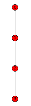
Figure 2: A path.

Consider, for example, the simple “path graph” $G=(\{0,1,2,3\},E)$ of 4 nodes as shown in Figure 2 where each node $i$ is connected the next node $i+1$. Recall that we also require each node to have a loop to itself (to reflect the nonzero diagonal entries of the nodal admittance matrix $Y$), so the edges in the graph are

$$E=\{(0,0),(0,1),(1,0),(1,1),(1,2),(2,1),(2,2),(2,3),(3,2),(3,3)\}.$$

By Definition 3, the points in $\Gamma_{G}$ are therefore

$$(\mathbf{e}_{0},\mathbf{e}_{0}),(\mathbf{e}_{0},\mathbf{e}_{1}),(\mathbf{e}_{1},\mathbf{e}_{0}),(\mathbf{e}_{1},\mathbf{e}_{1}),(\mathbf{e}_{1},\mathbf{e}_{2}),(\mathbf{e}_{2},\mathbf{e}_{1}),(\mathbf{e}_{2},\mathbf{e}_{2}),(\mathbf{e}_{2},\mathbf{e}_{3}),(\mathbf{e}_{3},\mathbf{e}_{2}),(\mathbf{e}_{3},\mathbf{e}_{3}).$$

Since $\boldsymbol{0}$ is already included in $\Gamma_{G}$, the symmetric adjacency polytope $\nabla_{G}$ is precisely the convex hull of $\Gamma_{G}$. With programs for computing volume of convex polytopes to be listed in §3.3, one can easily obtain that $\mu_{G}=\operatorname{NVol}_{6}(\nabla_{G})=\operatorname{NVol}_{6}(\operatorname{conv}\Gamma_{G})=8$. That is, the algebraic load flow equation for such a path graph has at most 8 isolated non-deficient complex solutions.

It is quite easy to understand the situation under which the introduction of a new connection in the power network will change the AP bound: Since the AP bound is formulated in terms of the volume of a polytope which is nondecreasing (i.e., it will either increase or remain unchanged when new points are added), this upper bound must also be nondecreasing with respect to the additions of new connections.

Theorem 5.

For a graph $G=(B,E)$ and two of its nodes $i$ and $j$ that are not directly connected (i.e., $(i,j)\notin E$), let $G^{\prime}=(B,E\cup\{(i,j)\})$ be the new graph constructed by adding the edge between $i$ and $j$ to $G$. Then

$$\mu_{G}\leq\mu_{G^{\prime}}.$$

Moreover, if $\{(\mathbf{e}_{i},\mathbf{e}_{j}),(\mathbf{e}_{j},\mathbf{e}_{i})\}\subset\nabla_{G}$ then

$$\mu_{G}=\mu_{G^{\prime}}.$$

Proof.

Recall that each edge in a graph contributes certain points (which may or may not be vertices) in the construction of the symmetric adjacency polytope. Since the edges of $G$ is a subset of the edges of $G^{\prime}$, we can see that $\nabla_{G}\subseteq\nabla_{G^{\prime}}$ with the equality hold precisely when the points contributed by $(i,j)$ are already inside $\nabla_{G}$. With these observations in mind, both parts of this theorem are direct implications of normalized volume being nondecreasing. ∎

Based on this observation, it can be shown that the AP bound is never more than the BBLSY bound. This is essentially our alternative proof of the BBLSY bound:

Theorem 6.

For a graph $G=(B,E)$, let $|B|=n+1$. Then, $\mu_{G}\leq\binom{2n}{n}$

Proof.

Fixing the set of buses, Theorem 5 states that the AP bound is nondecreasing as new edges are added to the graph. Consequently, the AP bound for any network constructed from this set of buses is bounded above by the AP bound for the graph with most edges, that is, a complete graph. It is easy to verify that for a complete graph $G=(B,E)$ (with loops), $\nabla_{G}\subseteq(\operatorname{conv}A)+(\operatorname{conv}B)$ where

$$A =\left\{\mathbf{e}_{0},\mathbf{e}_{1},\mathbf{e}_{2},\ldots\,\mathbf{e}_{n}\right\} B =\left\{\mathbf{e}_{0},\mathbf{e}_{n+1},\mathbf{e}_{n+2},\ldots\,\mathbf{e}_{2n}\right\}$$ (6)

and $(\operatorname{conv}A)+(\operatorname{conv}B)$ denotes the Minkowski sum of the two polytopes $(\operatorname{conv}A)$ and $(\operatorname{conv}B)$. Note that both $(\operatorname{conv}A)$ and $(\operatorname{conv}B)$ are $n$-dimensional. Then by multi-linearity of mixed volume with respect to Minkowski sum,

$$\operatorname{NVol}((\operatorname{conv}A)+(\operatorname{conv}B)) =\sum_{k=0}^{2n}\binom{2n}{k}MV((convA)^{(k)},(convB)^{(2n-k)})$$

$$=\binom{2n}{n}MV((convA)^{(n)},(convB)^{(n)})$$

$$=\binom{2n}{n}$$

∎

We conclude this section with a reiteration of the various root counts involved in the discussion. Recall that for a power network $G=(B,E)$, the number of isolated non-deficient solutions of the original (non-algebraic) load flow equation (1) (physical solutions), the number of isolated complex solutions of the algebraic load flow equation (5) in $(\mathbb{C}\setminus\{0\})^{2n}$, the BKK bound provided by Theorem 1, the AP bound given in Theorem 4, the BBLSY bound given in [3, 42], and the CB number are related as follows:

$$\parbox{38.74988pt}{\centering Physical \\ solution \\ count\@add@centering}\;\leq\;\parbox{38.74988pt}{\centering Complex \\ solution \\ count\@add@centering}\;\leq\;\parbox{30.1388pt}{\centering BKK \\ bound\@add@centering}\;\leq\;\parbox{30.1388pt}{\centering AP \\ bound\@add@centering}\;\leq\;\parbox{34.44434pt}{\centering BBLSY \\ bound\@add@centering}\;\leq\;\parbox{38.74988pt}{\centering CB \\ bound\@add@centering}$$

3.3 Computing BKK and AP bounds

The BKK bound, can be computed by using efficient software packages such as DEMiCs [51], Gfan [32], MixedVol [22], MixedVol-2.0 [39]. For larger power networks involving many buses, the induced algebraic load flow equation may contain a large number of terms. Parallel computing technology will be essential in the computation of the BKK bounds for such large scale polynomial systems. MixedVol-3 [13, 14] (with an improved version integrated in Hom4PS-3 [12]) is capable of computing the BKK bound for large polynomial systems in parallel on a wide range of hardware architectures including multi-core systems, NUMA systems, and computer clusters. As noted in Remark 1, however, there is built-in level of redundancy in the Newton polytopes (see Appendix A) of the algebraic load flow equations. The formulation of the AP bound takes advantage of this natural redundancy and can generally be computed much more easily than the BKK bound for larger power networks. Since the AP bound is formulated in terms of the volume of a convex polytope (the symmetric AP), any software that can compute such volume exactly can be used to provide this bound. A survey on the various algorithms for exact volume computation can be found in [6]. A particularly versatile software package that utilizes a wide range of algorithms is the Vinci program [21].

3.4 Homotopy methods for solving load flow equations

The previous sections described two upper bounds — the BKK bound and the AP bound — for the number of isolated non-deficient complex solutions of the algebraic load flow equation induced by a given network topology. It is worth reiterating that the BKK bound is more than just an upper bound: As shown in Theorem 2, it is actually the maximum for the given network topology in the sense that there always exits some choice of the admittance matrix $Y$ (and $S$) for which the total number of isolated non-deficient complex solutions is exactly the BKK bound. While the AP bound, in general, may be larger than the BKK bound, as we shall show in §4, the two coincide for all the networks we have investigated in the present work. The family of numerical methods known as homotopy methods have been proved to be a robust and efficient approach for solving algebraic load flow equations. One great strength of these methods lies in the pleasantly parallel nature: in principle, each solution can be computed independently. This feature is of particular importance in dealing with larger power networks containing many buses and connections (hence more complicated equations). It is therefore a natural question to ask: is there a homotopy method that can solve the algebraic load flow equation by tracking BKK bound number of homotopy paths? This section establishes the answer in the affirmative.

This homotopy method is the polyhedral homotopy method developed in [28]. Here we briefly state the construction. We choose a pair of random (rational) numbers $\omega_{ij}$ and $\omega_{ij}^{\prime}$ for each $i,j=1,\dots,n$. With these we define the homotopy function

$$H_{G,Y}(v_{1},\dots,v_{n},u_{1},\dots,u_{n},t)=\begin{cases}\sum_{k=0}^{n}Y_{1k}\,(t)v_{1}u_{k}t^{\omega_{1k}}-S_{1}(t)\\ \quad\vdots\\ \sum_{k=0}^{n}Y_{nk}(t)v_{n}u_{k}t^{\omega_{nk}}-S_{n}(t)\\[6.45831pt] \sum_{k=0}^{n}Y_{1k}^{\prime}\,(t)u_{1}v_{k}t^{\omega_{k1}^{\prime}}-S_{1}^{\prime}(t)\\ \quad\vdots\\ \sum_{k=0}^{n}Y_{nk}^{\prime}(t)u_{n}v_{k}t^{\omega_{kn}^{\prime}}-S_{n}^{\prime}(t).\end{cases}$$ (7)

where

$$Y_{ij}(t) =(1-t)Z_{ij}+tY_{ij}^{*} S_{i}(t) =(1-t)W_{i}+S_{i}$$

$$Y_{ij}^{\prime}(t) =(1-t)Z_{ij}^{\prime}+tY_{ij} S_{i}^{\prime}(t) =(1-t)W_{i}^{\prime}+S_{i}^{*}$$

and $(Z_{ij})$ and $(Z_{ij}^{\prime})$ are randomly chosen complex matrices of the same size as $Y$ and $W=(W_{i})$ and $W^{\prime}=(W_{i}^{\prime})$ are two random complex vectors in $\mathbb{C}^{n}$.

Clearly $H_{G,Y}(\mathbf{v},\mathbf{u},1)\equiv P_{G,Y}(\mathbf{v},\mathbf{u})$. For generic choice of $Z$, $Z^{\prime}$, $W$, $W^{\prime}$, $\omega$ and $\omega^{\prime}$, it can be shown that fixing any $t\in(0,1)$, the non-deficient solutions of $H_{G,Y}(\mathbf{v},\mathbf{u},t)=\boldsymbol{0}$ are all isolated and the total number is exactly the BKK bound. Moreover, as $t$ varies within $(0,1)$, the corresponding solutions of $H_{G,Y}(\mathbf{v},\mathbf{u},t)=\boldsymbol{0}$ also vary smoothly forming smooth solution paths that collectively reach all the desired solutions of the algebraic load flow equation $P_{G,Y}(\mathbf{v},\mathbf{u})=\boldsymbol{0}$. See Figure 1 for a schematic illustration. Thus, once the “starting points” of each solution path at $t=0$ are found, standard numerical continuation techniques can be used to track the solution paths and reach all the isolated non-deficient complex solutions.

Figure 1: The solution paths defined by $H_{G,Y}(\mathbf{v},\mathbf{u},t)=\boldsymbol{0}$.

An apparent difficulty is the identifications of the “starting points”. After all, at $t=0$, $H_{G,Y}(\mathbf{u},\mathbf{v},t)$ either becomes constant or undefined since each of its nonconstant term contains a power of $t$. This, fortunately, is surmounted via a device known as mixed cells which are themselves the by-product of the computation of the BKK bound. The technical detail is outside the scope of the present article, we therefore refer to standard references such as [28, 41]. The application of the polyhedral homotopy to load flow equations will be explored in future works, here we simply emphasize that with the polyhedral homotopy method, the number of solution paths one needs to track is precisely the BKK bound of the particular polynomial formulation of the load flow equations that we have used (eq. (5)) — the best possible network topology-based complex solution bound.

4 Solution bound for certain power networks

In this section we provide concrete computation results for the BKK bound and the AP bound described above when applied to specific graphs. We should reiterate that we require all the graphs to have self-loops for each node to reflect the nonzero diagonal entries of the nodal admittance matrix $Y$. In all cases, the BKK and the AP bounds are computed via MixedVol-3 [13, 14]. Complex solutions count of specific load flow systems are computed by actually solving the systems via Hom4PS-3 [11, 12] which implements the polyhedral homotopy method described above.

For comparison, in each case we show the “5-way comparison” among the complex solution count, BKK bound, AP bound, the BBLSY Bound, and the CB number. Here, “complex solution count” refers to the number of isolated complex solutions of (5) in $(\mathbb{C}\setminus\{0\})^{2n}$ where $n$ is number of non-reference nodes. Since the actual complex solution count may depend on the coefficients ($Y_{ij}$ and $S_{i}$ in (5)), they are computed based on a sample of randomly chosen set of coefficients for each graph.

4.1 Paths

We first consider an extremely sparsely connected family of graphs – path graphs. In a path graph $G=(B,E)$ with nodes $0,1,\dots,n$ where $n=|B|-1$ (the number of non-reference nodes), a node $i$ is connected to two of its neighbors $i+1$ and $i-1$, with the exceptions that node $0$ is only connected to node 1 and the last node, node $n$, is only connected to node $n-1$.

Table 1 shows the “5-way comparison” described above. It is important to note that in all cases computed (100 in total, with 10 random admittance matrices chosen for each $|B|$), the actual complex solution count, the BKK bound, and the AP bound are exactly the same.

$|B|$	2	3	4	5	6	7	8	9	10	11	12
Solutions	2	4	8	16	32	64	128	256	512	1024	2048
BKK	2	4	8	16	32	64	128	256	512	1024	2048
AP	2	4	8	16	32	64	128	256	512	1024	2048
BBLSY	2	6	20	70	252	924	3432	12870	48620	184756	705432
CB	4	16	64	256	1024	4096	16384	65536	262144	1048576	4194304

Table 1: The “5-way comparison” of the solution bounds for path graphs of size 2–12.

4.2 Rings

By joining the two ends of a path graph studied above, a “ring graph” is obtained. More precisely, in a ring $G=(B,E)$ with nodes $0,1,\dots,n$ where $n=|B|-1$, a node $i$ is connected to two of its neighbors $i+1$ and $i-1$, and node reference node, node $0$ is connected to node $n$. See, for example, the graph shown in Figure 3(a). Table 2 shows the similar “5-way comparison”. Again, in all cases computed (100 in total, with 10 random admittance matrices chosen for each $|B|$), the actual complex solution count, the BKK bound, and the AP bound are all exactly the same.

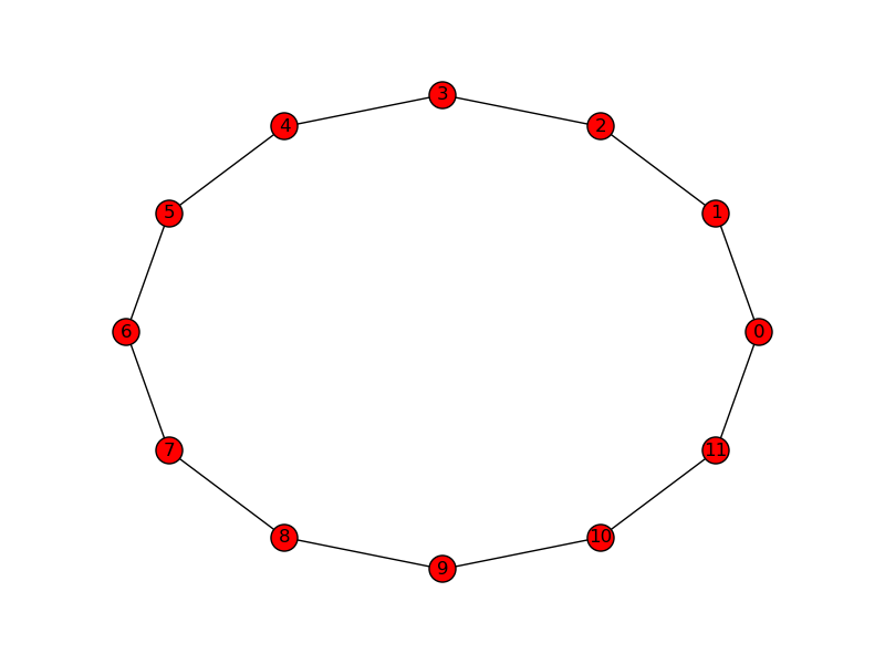
(a) A ring.

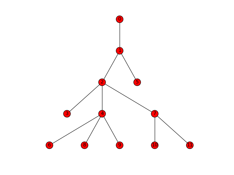
(b) A random tree

$|B|$	2	3	4	5	6	7	8	9	10	11	12
Solutions	2	6	16	40	96	224	512	1152	2560	5632	12288
BKK	2	6	16	40	96	224	512	1152	2560	5632	12288
AP	2	6	16	40	96	224	512	1152	2560	5632	12288
BBLSY	2	6	20	70	252	924	3432	12870	48620	184756	705432
CB	4	16	64	256	1024	4096	16384	65536	262144	1048576	4194304

Table 2: The “5-way comparison” of solution bounds for ring graphs of size 2–12.

4.3 Random trees

Since distribution networks often have structures of trees, randomly generated trees may actually resemble some realistic power networks. To get a reasonable sample size, tree graphs with $|B|=3,\dots,13$ are studied. For each of the sizes 10 trees are randomly generated (see, for example, the trees shown in Figure 3(b)). For each of these trees, 100 set of random $Y$ matrices are assigned. Therefore for each given size $|B|$, 1000 polynomial systems are generated (a total of 10000 systems for $|B|=3,\dots,13$). Table 3 shows the similar “5-way comparison” used above.

$|B|$	3	4	5	6	7	8	9	10	11	12	13
Solutions	4	8	16	32	64	128	256	512	1024	2048	4096
BKK	4	8	16	32	64	128	256	512	1024	2048	4096
AP	4	8	16	32	64	128	256	512	1024	2048	4096
BBLSY	6	20	70	252	924	3432	12870	48620	184756	705432	2704156
CB	16	64	256	1024	4096	16384	65536	262144	1048576	4194304	16777216

Table 3: The “5-way comparison” for randomly generated trees of given sizes.

4.4 Clusters

Real power networks generally exhibit certain level of “clustering”, that is, certain subset of buses are densely connected while on a larger scale, the connections among such subsets are sparse. Here for simplicity, we focus on the most extreme cases where a larger network is created by joining completely connected subnetworks. This section lists concrete results of the BKK and AP bounds for certain simple types of clusters. For comparison, in each case we only show the “3-way comparison” among the BKK bound, AP bound, and the BBLSY bound (due to the large amount of data).

4.4.1 Subnetworks sharing nodes

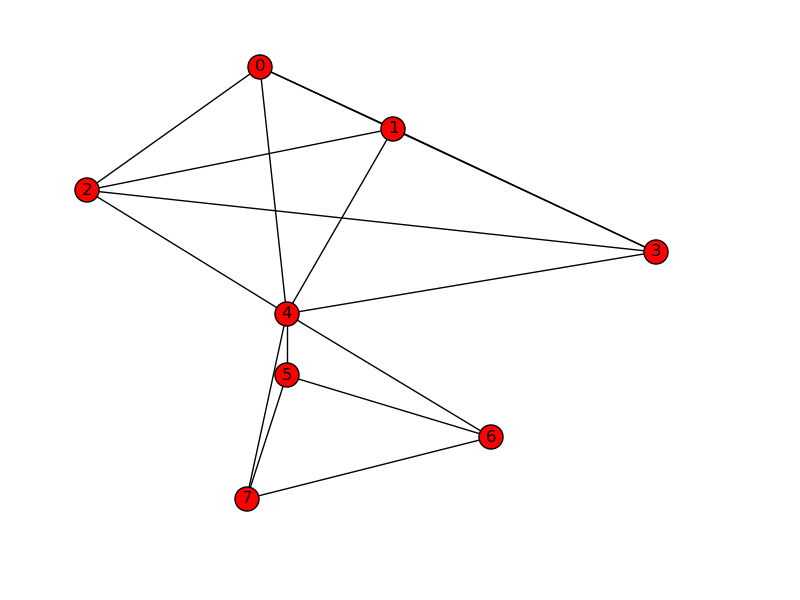
(a) Sharing one node

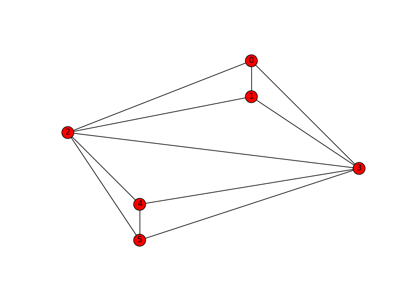
(b) Sharing two nodes

Figure 4: Completely connected subgraphs sharing common nodes.

First, these subnetworks can be jointed by sharing common nodes. See, for example, the networks shown in Figure 4. Table 4 shows the “3-way comparison” for cases where two completely connected subnetworks share a single (non-reference) common bus. These cases have been studied in [26]. Our computational results agree with their assertion. Table 5 shows the similar “3-way comparison” for cases where two completely connected subnetworks share two (non-reference) common bus. These cases have been extensively studied in [53] via numerical methods. The results and conjectures in that work are precisely reproduced by our computation. For larger networks, the AP bounds are generally much easier to compute than the BKK bound using existing implementations. In Table 6 and 7, we show the AP bounds for the above referenced clusters.

$c_{1}\backslash c_{2}$	2	3	4	5	6
2	4/4/6	12/12/20	40/40/70	140/140/252	504/504/924
3	12/12/20	36/36/70	120/120/252	420/420/924	1512/1512/3432
4	40/40/70	120/120/252	400/400/924	1400/1400/3432	5040/5040/12870
5	140/140/252	420/420/924	1400/1400/3432	4900/4900/12870	17640/17640/48620
6	504/504/924	1512/1512/3432	5040/5040/12870	17640/17640/48620	63504/63504/184756

Table 4: The “3-way comparison” for two completely connected subnetworks of sizes $c_{1}$ and $c_{2}$ respectively sharing a single common non-reference nodes.

$c_{1}\backslash c_{2}$	2	3	4	5	6
2	2/2/2	6/6/6	20/20/20	70/70/70	252/252/252
3	6/6/6	18/18/20	60/60/70	210/210/252	756/756/924
4	20/20/20	60/60/70	200/200/252	700/700/924	2520/2520/3432
5	70/70/70	210/210/252	700/700/924	2450/2450/3432	8820/8820/12870
6	252/252/252	756/756/924	2520/2520/3432	8820/8820/12870	31752/31752/48620

Table 5: The “3-way comparison” for two completely connected subnetworks of sizes $c_{1}$ and $c_{2}$ respectively sharing two common non-reference nodes.

$c_{1}\backslash c_{2}$	2	3	4	5	6	7	8
2	4	12	40	140	504	1848	6864
3	12	36	120	420	1512	5544	20592
4	40	120	400	1400	5040	18480	68640
5	140	420	1400	4900	17640	64680	240240
6	504	1512	5040	17640	63504	232848	864864
7	1848	5544	18480	64680	232848	853776	3171168
8	6864	20592	68640	240240	864864	3171168	11778624

Table 6: The AP bounds for graphs consisting of two cliques of size $c_{1}$ and $c_{2}$ respectively sharing a single common non-reference node.

$c_{1}\backslash c_{2}$	2	3	4	5	6	7	8
2	2	6	20	70	252	924	3432
3	6	18	60	210	756	2772	10296
4	20	60	200	700	2520	9240	34320
5	70	210	700	2450	8820	32340	120120
6	252	756	2520	8820	31752	116424	432432
7	924	2772	9240	32340	116424	426888	1585584
8	3432	10296	34320	120120	432432	1585584	5889312

Table 7: The AP bounds for graphs consisting of two cliques, of size $c_{1}$ and $c_{2}$ respectively sharing two common non-reference nodes.

4.4.2 Completely connected subnetworks connected by edges

We now consider cases where completely connected subnetworks are connected by edges. For example, Figure 5(a) shows a network that consists of two cliques of size four and five respectively connected by a single edge. Table 8 shows the AP bounds for networks created from joining two completely connected subnetworks by a single edge.

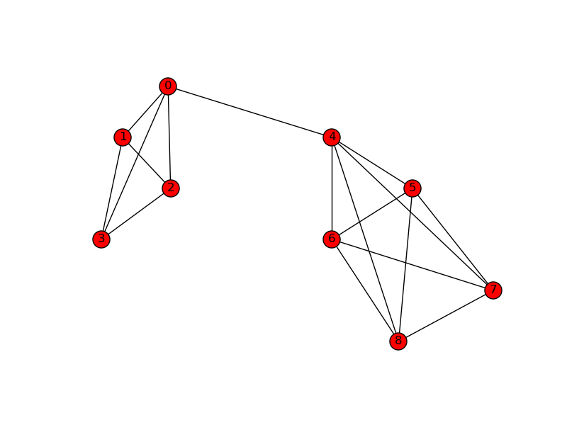
(a) Two completely connected subnetworks jointed via a single edge.

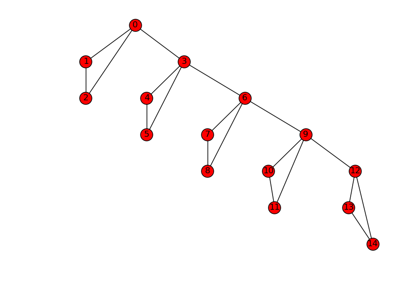
(b) A network containing several subnetworks linked together via edges.

Figure 5: Completely connected subnetworks connected by edges

$c_{1}\backslash c_{2}$	1	2	3	4	5	6	7	8	9	10
1		4	12	40	140	504	1848	6864	25740	97240
2	4	8	24	80	280	1008	3696	13728	51480	194480
3	12	24	72	240	840	3024	11088	41184	154440	583440
4	40	80	240	800	2800	10080	36960	137280	514800	1944800
5	140	280	840	2800	9800	35280	129360	480480	1801800
6	504	1008	3024	10080	35280	127008	465696	1729728
7	1848	3696	11088	36960	129360	465696	1707552
8	6864	13728	41184	137280	480480	1729728
9	25740	51480	154440	514800	1801800
10	97240	194480	583440	1944800

Table 8: The AP bound of graphs consisting of two cliques of size $c_{1}$ and $c_{2}$ joint by a single edge.

Table 9 shows the AP bounds of the more general cases where the networks consist of multiple completely connected subnetworks of the same sizes connected via edges to form chains-like structure. See, for example, the network shown in Figure 5(b) where five cliques each of size three are connected via edges that, on a macro level, resembles a chain.

$c\backslash m$	1	2	3	4	5	6	7	8
	1	2	3	4	5	6	7	8
1		2	4	8	16	32	64	128
2	2	8	32	128	512	2048	8192	32768
3	6	72	864	10368	124416	1492992	17915904
4	20	800	32000	1280000
5	70	9800	1372000
6	252	127008
7	924	1707552
8	3432

Table 9: The AP bound for graphs consisting of $n$ cliques each of size $c$.

5 IEEE 14 bus system

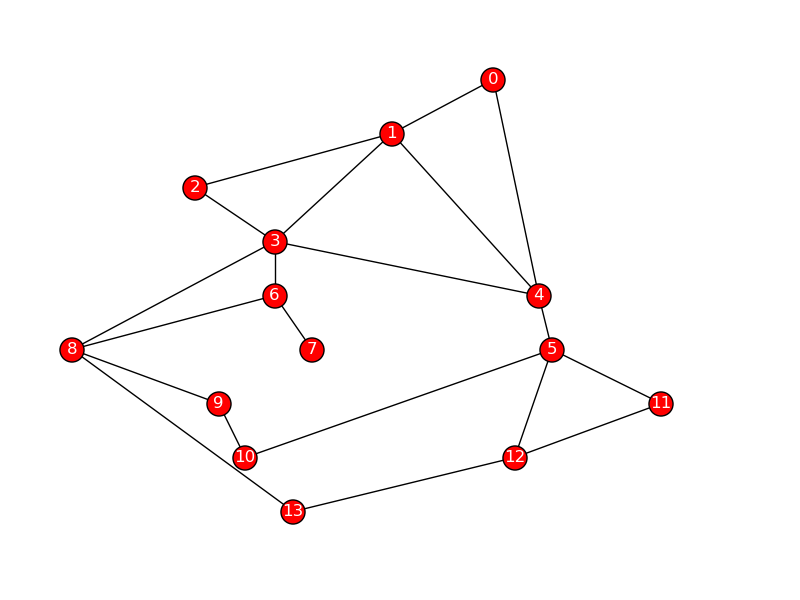
Figure 6: IEEE 14 bus system

The IEEE 14 bus system (the network toopology shown in Figure 6), representing a portion of the power system of the Midwestern U.S.A. in the 1960s, is a widely used benchmark system in testing the efficiency of different solvers for load flow equations.

Here we show that the isolated complex solution count, BKK bound, and AP bound are much smaller than previously studied solution bounds. In particular, the BKK bound in our formulation of the load flow equations is 427680. This means the polyhedral homotopy method described in Sec. 3.4 need to trace at most 427680 paths to obtain all isolated non-deficient complex solutions, which compared with the BKK bound in a previous formulation of the load flow equations [49], 49283072, is around a factor 115 of reduction. This is well within the reach of modern polyhedral homotopy implementations. In particular, with a random choice of the $Y$-matrix, Hom4PS-3 [11, 12] was able to find all solutions in less than 5 minutes (around 297 seconds) on a single workstation (with two Intel Xeon processor).

Solutions	427680
BKK bound	427680
AP bound	427680
BKK-MNT[49]	49283072
BBLSY bound	10400600
CB bound	67108864

Table 10: Solution bounds for the IEEE 14-bus topology, with generic complex coefficients. BKK-MNT is the BKK bound with a different polynomial formulation [49].

6 Conclusion and Outlook

Solutions of the load flow equations play an important role in design and operations of power systems and a huge amount of research activities have been focused on developing efficient computational methods to solve the load flow equations [48]. In this paper we focus on computing a tight upper bound on the number of load flow solutions for the following reasons: the NPHC method [60, 41] introduced in power systems areas in [49, 8, 9, 47, 53] requires an upper bound on the number of isolated (complex) solutions of the system. The CB bound or most of the other existing upper bounds, and in particular the BBLSY bound [3, 42], do not capture the network topology[53] of the power system into account. To make the computation of the NPHC method efficient, and to provide a definitive stopping criterion for other iterative methods, one has to come up with a tighter upper bound on the number of isolated complex solutions.

In this paper, for technical reasons, we ignore the physically less likely solutions at which at least one of the voltages is zero. We described a specific version of the algebraic formulation of the load flow equations and a corresponding tighter upper bound known as the BKK bound. We showed that there exists at least some generic parameter values for which the BKK bound is attainable.

Another novel feature in this paper is the introduction of a novel bound, called an AP, for sparse systems. With this bound, we proved one of our main theorems, Theorem 4, which gives a more explicit bound on the number of complex solutions. The new bound is computationally much more tractable for large systems compared to the BKK bound.

Our bounds not only give the precise number of complex solutions for the given power system, but also provide a particular specialization of the NPHC method that in turn achieves all the solutions for the system but more efficiently than the previous ones that are based on the crude bounds. We examined our results on upper bounds on the number of complex solutions with the actual number of complex solutions obtained with the help of the polyhedral NPHC method for various cases including complete graphs; path graphs; ring graphs; wheel graphs; random tree graphs; graphs having two cliques sharing exactly one, two and three nodes; graphs having two cliques both connected by a single edge; graphs with multiple cliques of equal size connected via edges, and the IEEE standard 14-bus system. In all the instances we have tested, we find that (1) the BKK bound is always equal to the adjacency bound, and (2) the BKK bound is always equal to the actual number of complex solutions, i.e., the BKK or the AP bound are the actual number of isolated complex solutions for generic coefficients and completely capture the specific network topology of the given power systems. A proof supporting the numerical results will be published elsewhere. Our numerical investigations reproduced all the previously known results [3, 27, 53]. In addition, we provide further novel results for aforementioned list of graphs.

We emphasis that the BKK bound is dependent on the polynomial formulation used to compute it, though the number of complex solutions and number of physical solutions are obviously independent of the polynomial formulations. The phrase ”BKK bound” throughout the paper, unless specified otherwise, is computed from the polynomial formulation we have described in this paper (given in eq. (5)). In other words, our polynomial formulation seems optimal since the BKK bound computed using it is generically equal to the number of isolated complex solutions. To give an example, for the IEEE standard 14-bus system, the BKK using a previous formulation was $49,283,072$, whereas the BKK in the present formulation is $427,680$, i.e., a factor of around $115$ reduction with our present formulation.

Our results open up several future directions: though a less likely case, extending our results to the situtation where at least one of the voltages is zero would further complete the discussion on number of complex solutions. Further refinement will be accomplished by computing or estimating the number of physical solutions, and analysing their stability properties for different network topologies. Investigating for which parameter values the number of physical solutions is equal or at least of the same order of magnitude as the number of complex solutions of the systems will also provide a better tool to analyse efficiencies of different computational methods: For example, for the 3 nodes complete graph case, it is known that the number of real solutions does attain the tight-most upper bound on the number of complex solutions, $6$[61, 2, 35]. However, for $4$ nodes complete graph case, so far parameter points with only $14$ physical solutions are known as opposed to $20$ complex solutions [3]. This has an important consequences on the tracing-methods for solving load flow equations such as proposed in Refs. [44, 40]. Leaving aside the lack of proof for guaranteeing all the physical solutions of the load flow equations in the tracing-methods, for such parameter points at which the number of physical solutions is equal or of the same order of magnitude as the BKK bound, the number of traces the method has to go through will be equivalent to the polyhedral NPHC method will also have to go through. Hence, in such cases, there will be no gain even if one ignores the guarantee to find all solutions that the NPHC method provides. On the other hand, our bounds can provide the necessary stopping criterion to the tracing-methods and hence the two methods may complement each other in some cases.

Appendix A Mixed volume and BKK bound

Given $m$ convex polytopes $Q_{1},\dots,Q_{m}\subset\mathbb{R}^{n}$ and $m$ positive real numbers $\lambda_{1},\dots,\lambda_{m}$ with $m\leq n$ Minkowski’s Theorem [50] states that the $n$-dimensional volume of the Minkowski sum [50, 24].

$$\lambda_{1}Q_{1}+\cdots+\lambda_{n}Q_{n}=\{\;\lambda_{1}\mathbf{q}_{1}+\cdots+\lambda_{n}\mathbf{q}_{n}\mid\mathbf{q}_{i}\in Q_{i}\text{ for }i=1,\dots,n\;\}$$

is a homogeneous polynomial of degree $n$ in the variables $\lambda_{1},\dots,\lambda_{n}$. For a $m$-tuple of nonnegative integers $(k_{1},\dots,k_{m})$, the coefficient associated with the monomial $\lambda_{1}^{k_{1}}\cdots\lambda_{m}^{k_{m}}$ is known as the mixed volume [24, 50] of type $(k_{1},\dots,k_{m})$. Mixed volume of type $(1,\dots,1)$ is often simply referred to as the mixed volume. As a common convention, the mixed volume involving two shapes in $\mathbb{R}^{2}$ are usually called mixed area instead.

The BKK bound is formulated in terms of mixed volume. We start with an example (used in [28]): With $\mathbf{x}=(x_{1},x_{2})$, let $P(\mathbf{x})$ be the polynomial system

$$p_{1}(\mathbf{x}) =c_{11}x_{1}x_{2}+c_{12}x_{1}+c_{13}x_{2}+c_{14}$$

$$p_{2}(\mathbf{x}) =c_{21}x_{1}x_{2}^{2}+c_{22}x_{1}^{2}x_{2}+c_{23}$$

Here, $c_{ij}$’s are nonzero coefficients. The formal expressions for the monomials in $p_{1}$ are $x_{1}x_{2}=x_{1}^{1}x_{2}^{1}$, $x_{1}=x_{1}^{1}x_{2}^{0}$, $x_{2}=x_{1}^{0}x_{2}^{1}$ and $1=x_{1}^{0}x_{2}^{0}$. Considering the exponents of each monomial as a point on the plane, the set of exponent points $S_{1}=\{a=(0,0),\;b=(1,0),\;c=(1,1),\;d=(0,1)\}$ is called the support of $p_{1}$, and its convex hull $Q_{1}=\operatorname{conv}(S_{1})$ is called the Newton polygon of $p_{1}$. Similarly, the support of $p_{2}$ is $S_{2}=\{e=(0,0),\;f=(2,1),\;g=(1,2)\}$ and its Newton polygon is $Q_{2}=\operatorname{conv}(S_{2})$. The two newton polygons are shown in Figure 7(a) and 7(b) respectively. The mixed area of $Q_{1}$ and $Q_{2}$ can be intuitively taken as the area within the Minkowski sum $Q_{1}+Q_{2}$ contributed by “mixing” of the two shapes. From Figure 7(c), it is easy to see that $Q_{1}+Q_{2}$ contains copies of $Q_{1}$ and $Q_{2}$. The rest (the shaded region) are resulted from the “mixing effect” of edges from both $Q_{1}$ and $Q_{2}$ in constructing the Minkowski sum. The total area of these regions is the mixed area.

(a) $Q_{1}$

(b) $Q_{2}$

(c) The Minkowski sum $Q_{1}+Q_{2}$

Figure 7: The Newton polygons of $p_{1}$ and $p_{2}$ along with their Minkowski sum and a graphical depiction of the mixed volume (mixed area).

In general, given a polynomial system $P=(p_{1},\dots,p_{n})$ of the form

$$\left(\sum_{\mathbf{a}\in S_{1}}c_{1,\mathbf{a}}\mathbf{x}^{\mathbf{a}},\;\dots\;,\sum_{\mathbf{a}\in S_{n}}c_{n,\mathbf{a}}\mathbf{x}^{\mathbf{a}}\right)$$

where $\mathbf{x}=(x_{1},\dots,x_{n})$ and $S_{1},\dots,S_{n}$ are fixed subsets of $\mathbb{Z}^{n}$ called the support of $p_{1},\dots,p_{n}$ respectively. Note that here with $\mathbf{a}=(a_{1},\dots,a_{n})$ we use the notation $\mathbf{x}^{\mathbf{a}}=x_{1}^{a_{1}}\cdots x_{n}^{a_{n}}$ for a monomial. The convex hull $Q_{j}=\operatorname{conv}(S_{j})$ in $\mathbb{R}^{n}$ is called the Newton polytope of $p_{j}$. In this context, the BKK bound is the mixed volume of the Newton polytopes $Q_{1},\dots,Q_{n}$.

Appendix B Zariski openness

Part (B) of Theorem 1 states that ignoring the conjugate relations among the coefficients, the set of coefficients for which the upper bound given by Theorem 1 part (A) hold exactly is at least a nonempty “Zariski open” set. This “Zariski openness” can be characterized as follows: If we replace $Y_{jk}^{*}$ and $S_{j}^{*}$ in (5) by independent coefficients $Y_{jk}^{\prime}$ and $S_{j}^{\prime}$, then there exists a nonzero polynomial $D$ in the variables $\{Y_{jk},Y_{jk}^{\prime},S_{j},S_{j}^{\prime}\}$ such that $D\neq 0$ implies the BKK bound is exact.

Appendix C The polarization lemma

The proof for Theorem 2 hinges on a key lemma in the theory of complex variables that is sometimes referred to as the polarization lemma:

Lemma 7.

Suppose that $H:(\mathbb{C}\setminus\{0\})^{n}\times(\mathbb{C}\setminus\{0\})^{n}\to\mathbb{C}$ is a holomorphic function of the $2n$ complex variables $(\mathbf{z},\mathbf{w})$, and that $H(\mathbf{z},\mathbf{z}^{*})=0$ for all $\mathbf{z}\in(\mathbb{C}\setminus\{0\})^{n}$. Then, $H(\mathbf{z},\mathbf{w})=0$ for all $(\mathbf{z},\mathbf{w})\in(\mathbb{C}\setminus\{0\})^{n}\times(\mathbb{C}\setminus\{0\})^{n}$.

This lemma has its roots in the works of W. Wirtinger. Here we refer to [17] for a direct proof.

References

- [1] Venkataramana Ajjarapu and Colin Christy, The continuation power flow: a tool for steady state voltage stability analysis, Power Systems, IEEE Transactions on, 7 (1992), pp. 416–423.
- [2] J Baillieul, The critical point analysis of electric power systems, in The 23rd IEEE Conference on Decision and Control, no. 23, 1984, pp. 154–159.
- [3] J. Baillieul and C.I. Byrne, Geometric Critical Point Analysis of Lossless Power System Models, IEEE Trans. Circuits Syst., 29 (1982).
- [4] David N Bernshtein, The number of roots of a system of equations, Funct. Anal. Its Appl., 9 (1975), pp. 183–185.
- [5] D.M. Bromberg, M. Jereminov, X. Li, G. Hug, and L. Pileggi, An Equivalent Circuit Formulation of the Power Flow Problem with Current and Voltage State Variables, in IEEE Eindhoven PowerTech, Jun. 2015.
- [6] Benno Büeler, Andreas Enge, and Komei Fukuda, Exact Volume Computation for Polytopes: A Practical Study, in Polytopes — Combinatorics and Computation, Gil Kalai and Günter M. Ziegler, eds., no. 29 in DMV Seminar, Birkhäuser Basel, Jan. 2000, pp. 131–154.
- [7] John Canny and J. Maurice Rojas, An optimal condition for determining the exact number of roots of a polynomial system, in Proceedings of the 1991 International Symposium on Symbolic and Algebraic Computation, ISSAC ’91, New York, NY, USA, 1991, ACM, pp. 96–102.
- [8] Souvik Chandra, Dhagash Mehta, and Aranya Chakrabortty, Exploring the impact of wind penetration on power system equilibrium using a numerical continuation approach, arXiv preprint arXiv:1409.7844, (2014).
- [9] , Equilibria analysis of power systems using a numerical homotopy method, in Power & Energy Society General Meeting, 2015 IEEE, IEEE, 2015, pp. 1–5.
- [10] H. Chen, Cascaded Stalling of Induction Motors in Fault-Induced Delayed Voltage Recovery (FIDVR), Masters Thesis, University of Wisconsin-Madison, Department of Electrical and Computer Engineering, (2011).
- [11] Tianran Chen, Tsung-Lin Lee, and Tien-Yien Li, Hom4PS-3: an numerical solver for polynomial systems using homotopy continuation methods.
- [12] , Hom4PS-3: A Parallel Numerical Solver for Systems of Polynomial Equations Based on Polyhedral Homotopy Continuation Methods, in Mathematical Software – ICMS 2014, Hoon Hong and Chee Yap, eds., no. 8592 in Lecture Notes in Computer Science, Springer Berlin Heidelberg, Jan. 2014, pp. 183–190.
- [13] , Mixed volume computation in parallel, Taiwan. J. Math., 18 (2014), pp. 93–114.
- [14] , Mixed cell computation in Hom4PS-3, Numer. Algebr. Geom. Spec. Issue J. Symb. Comput., ((To appear)).
- [15] Tianran Chen, Tien-Yien Li, and Xiaoshen Wang, Theoretical aspects of mixed volume computation via mixed subdivision, Commun. Inf. Syst., 14 (2014), pp. 213–242.
- [16] D. Cifuentes and P. Parrilo, Exploiting Chordal Structure in Polynomial Ideals: A Gröbner Bases Approach, Preprint: http://arxiv.org/abs/1411.1745, (2014).
- [17] John P. D’Angelo, Several Complex Variables and the Geometry of Real Hypersurfaces, CRC Press, Jan. 1993.
- [18] F. Dörfler and F. Bullo, Novel Insights into Lossless AC and DC Power Flow, in IEEE PES General Meeting, Jul. 2013.
- [19] P. Dreesen and B. De Moor, Polynomial Optimization Problems are Eigenvalue Problems, in Model-Based Control: Bridging Rigorous Theory and Advanced Technology, Paul M.J. Hof, Carsten Scherer, and Peter S.C. Heuberger, eds., Springer US, 2009, pp. 49–68.
- [20] K. Dvijotham, S. Low, and M. Chertkov, Solving the Power Flow Equations: A Monotone Operator Approach, Submitted. Preprint available: http://arxiv.org/abs/1506.08472, (2015).
- [21] Andreas Enge, Benno Büeler, and Komei Fukuda, VINCI: an easy to install C package that implements the state of the art algorithms for volume computation.
- [22] Tangan Gao, Tien-Yien Li, and Mengnien Wu, Algorithm 846: MixedVol: a software package for mixed-volume computation, ACM Trans. Math. Softw. TOMS, 31 (2005), pp. 555–560.
- [23] J.D. Glover, M.S. Sarma, and T.J. Overbye, Power System Analysis and Design, Cengage Learning, 2011.
- [24] H. Groemer, Minkowski addition and mixed volumes, Geom Dedicata, 6 (1977), pp. 141–163.
- [25] S.X. Guo and F.M.A. Salam, Determining the solutions of the load flow of power systems: Theoretical results and computer implementation, in , Proceedings of the 29th IEEE Conference on Decision and Control, 1990, Dec. 1990, pp. 1561–1566 vol.3.
- [26] S.X. Guo and F.M.A. Salam, Determining the Solutions of the Load Flow of Power Systems: Theoretical Results and Computer Implementation, in IEEE 29th Ann. Conf. Decis. Contr. (CDC), Dec. 1990, pp. 1561–1566.
- [27] , The Number of (Equilibrium) Steady-State Solutions of Models of Power Systems, IEEE Trans. Circuits Syst. I, Fundam. Theory Appl., 41 (1994), pp. 584–600.
- [28] B. Huber and B. Sturmfels, A polyhedral method for solving sparse polynomial systems, Math. Comput., 64 (1995), pp. 1541–1555.
- [29] , Bernstein’s theorem in affine space, Discrete Comput Geom, 17 (1997), pp. 137–141.
- [30] M. Ilic, Network Theoretic Conditions for Existence and Uniqueness of Steady State Solutions to Electric Power Circuits, in IEEE Int. Symp. Circuits Syst. (ISCAS), May 1992.
- [31] S. Iwamoto and Y. Tamura, A Load Flow Calculation Method for Ill-Conditioned Power Systems, IEEE Trans. Power App. Syst., PAS-100 (1981), pp. 1736–1743.
- [32] Anders N. Jensen, A Presentation of the Gfan Software, in Mathematical Software - ICMS 2006, Andrés Iglesias and Nobuki Takayama, eds., no. 4151 in Lecture Notes in Computer Science, Springer Berlin Heidelberg, Jan. 2006, pp. 222–224.
- [33] A.G. Khovanskii, Newton polyhedra and the genus of complete intersections, Funct. Anal. Its Appl., 12 (1978), pp. 38–46.
- [34] A. Klos and A. Kerner, The Non-Uniqueness of Load Flow Solution, in 5th Power Syst. Comput. Conf. (PSCC), 1975.
- [35] A Klos and J Wojcicka, Physical aspects of the nonuniqueness of load flow solutions, International Journal of Electrical Power & Energy Systems, 13 (1991), pp. 268–276.
- [36] Prabha Kundur, Neal J Balu, and Mark G Lauby, Power system stability and control, vol. 7, McGraw-hill New York, 1994.
- [37] A. G. Kushnirenko, Newton polytopes and the Bezout theorem, Funct Anal Its Appl, 10 (1976), pp. 233–235.
- [38] Jean-Bernard Lasserre, Moments, Positive Polynomials and Their Applications, vol. 1, Imperial College Press, 2010.
- [39] Tsung-Lin Lee and Tien-Yien Li, Mixed volume computation in solving polynomial systems, Contemp Math, 556 (2011), pp. 97–112.
- [40] B. Lesieutre and D. Wu, An Efficient Method to Locate All the Load Flow Solutions - Revisited, 53rd Annual Allerton Conference on Communication, Control, and Computing, Sept 29-Oct 2, (2015).
- [41] Tien-Yien Li, Numerical solution of polynomial systems by homotopy continuation methods, in Handbook of Numerical Analysis, P. G. Ciarlet, ed., vol. 11, North-Holland, 2003, pp. 209–304.
- [42] Tien-Yien Li, Tim Sauer, and James A. Yorke, Numerical solution of a class of deficient polynomial systems, SIAM J. Numer. Anal., 24 (1987), pp. 435–451.
- [43] C.-W. Liu, C.-S. Chang, J.-A. Jiang, and G.-H. Yeh, Toward a CPFLOW-based Algorithm to Compute All the Type-1 Load-Flow Solutions in Electric Power Systems, IEEE Trans. Circuits Syst. I, Reg. Papers, 52 (2005), pp. 625–630.
- [44] W. Ma and S. Thorp, An Efficient Algorithm to Locate All the Load Flow Solutions, IEEE Trans. Power Syst., 8 (1993), p. 1077.
- [45] R. Madani, J. Lavaei, and R. Baldick, Convexification of Power Flow Problem over Arbitrary Networks, IEEE 54th Ann. Conf. Decis. Contr. (CDC), (2015).
- [46] Jakub Marecek, Timothy McCoy, and Martin Mevissen, Power flow as an algebraic system, arXiv preprint arXiv:1412.8054, (2014).
- [47] Dhagash Mehta, Noah S Daleo, Florian Dörfler, and Jonathan D Hauenstein, Algebraic geometrization of the kuramoto model: Equilibria and stability analysis, Chaos: An Interdisciplinary Journal of Nonlinear Science, 25 (2015), p. 053103.
- [48] Dhagash Mehta, Daniel K Molzahn, and Konstantin Turitsyn, Recent advances in computational methods for the power flow equations, arXiv preprint arXiv:1510.00073, (2015).
- [49] D. Mehta, H. Nguyen, and K. Turitsyn, Numerical Polynomial Homotopy Continuation Method to Locate All The Power Flow Solutions, Preprint: http://arxiv.org/abs/1408.2732, (2014).
- [50] Hermann Minkowski, Theorie der Konvexen Körper, insbesondere Begrundung ihres Oberflachenbegriffs, Gesammelte Abh. Von Hermann Minkowski, 2 (1911), pp. 131–229.
- [51] Tomohiko Mizutani and Akiko Takeda, DEMiCs: A Software Package for Computing the Mixed Volume Via Dynamic Enumeration of all Mixed Cells, in Software for Algebraic Geometry, Michael Stillman, Jan Verschelde, and Nobuki Takayama, eds., no. 148 in The IMA Volumes in Mathematics and its Applications, Springer, Jan. 2008, pp. 59–79.
- [52] D.K. Molzahn, B.C. Lesieutre, and H. Chen, Counterexample to a Continuation-Based Algorithm for Finding All Power Flow Solutions, IEEE Trans. Power Syst., 28 (2013), pp. 564–565.
- [53] Daniel K Molzahn, Dhagash Mehta, and Matthew Niemerg, Toward topologically based upper bounds on the number of power flow solutions, arXiv preprint arXiv:1509.09227, (2015).
- [54] Antonio Montes and Jordi Castro, Solving the load flow problem using gröbner basis, ACM SIGSAM Bulletin, 29 (1995), pp. 1–13.
- [55] Alexander Morgan and Andrew Sommese, Computing all solutions to polynomial systems using homotopy continuation, Applied Mathematics and Computation, 24 (1987), pp. 115–138.
- [56] Alexander P. Morgan, Andrew J. Sommese, and Layne T. Watson, Finding all isolated solutions to polynomial systems using HOMPACK, ACM Trans Math Softw, 15 (1989), pp. 93–122.
- [57] H. Mori and A. Yuihara, Calculation of Multiple Power Flow Solutions with the Krawczyk Method, in IEEE Int. Symp. Circuits Syst. (ISCAS), 30 May - 2 Jun. 1999.
- [58] Hieu D Nguyen and Konstantin S Turitsyn, Appearance of multiple stable load flow solutions under power flow reversal conditions, in PES General Meeting— Conference & Exposition, 2014 IEEE, IEEE, 2014, pp. 1–5.
- [59] Jiaxin Ning, Wenzhong Gao, G. Radman, and J. Liu, The Application of the Groebner Basis Technique in Power Flow Study, in North American Power Symp. (NAPS), Oct. 2009.
- [60] A. J. Sommese and C. W. Wampler, The numerical solution of systems of polynomials arising in engineering and science, World Scientific Pub Co Inc, 2005.
- [61] Carlos J Tavora and Otto JM Smith, Equilibrium analysis of power systems, Power Apparatus and Systems, IEEE Transactions on, (1972), pp. 1131–1137.
- [62] J.S. Thorp and S.A. Naqavi, Load Flow Fractals, in IEEE 28th Ann. Conf. Decis. Contr. (CDC), Dec. 1989.
- [63] A. Trias, The Holomorphic Embedding Load Flow Method, in IEEE PES General Meeting, Jul. 2012.