Uncertainty Quantification for Cargo Hold Fires

Abstract

The purpose of this study is twofold – first, to introduce the application of high-order discontinuous Galerkin methods to buoyancy-driven cargo hold fire simulations; second, to explore statistical variation in the fluid dynamics of a cargo hold fire given parameterized uncertainty in the fire source location and temperature. Cargo hold fires represent a class of problems that require highly-accurate computational methods to simulate faithfully. Hence, we use an in-house discontinuous Galerkin code to treat these flows. Cargo hold fires also exhibit a large amount of uncertainty with respect to the boundary conditions. Thus, the second aim of this paper is to quantify the resulting uncertainty in the flow, using tools from the uncertainty quantification community to ensure that our efforts require a minimal number of simulations. We expect that the results of this study will provide statistical insight into the effects of fire location and temperature on cargo fires, and also assist in the optimization of fire detection system placement.

1 Introduction

Federal aviation regulations require that all large passenger aircraft have fire detection and suppression systems in all cargo compartments. Several different detection methods are generally used together, such as sensors for temperature, carbon monoxide, smoke particulate, radiation, and optical detection. These sensors are required to detect the fire within 60 seconds of fire ignition. Certification of these systems currently requires expensive ground and in-flight testing. Current fire detection certification focuses on experiments using a small fire in empty cargo holds, such as the narrow-body Boeing 707 fuselage located at the Federal Aviation Administration William J. Hughes Technical center in Atlantic City, New Jersey[1]. Simulating a single fire case is a well-posed problem and relatively straightforward, but of limited utility. Due to the costs associated with these types of experiments, testing a wide variety of fire sources, positions, and compartment cargo cluttering is not feasible.

CFD tools that can accurately simulate heat and particulate transfer in fire-induced flow in cargo holds can potentially reduce these certification costs by reducing the amount of experimental work necessary. Simulations can then be used to assess the effectiveness of a particular detector placement, as well as optimize their placement in a given cargo hold. The allure of CFD tools is the reduction of monetary costs associated with certification tests; however, a drawback is the associated computational expense. In light of this, an issue that needs to be addressed is how to accurately quantify the uncertainty associated with randomly variable boundary conditions (eg., fire source location or temperature) while using the least amount of CFD simulations possible.

This work has two main objectives. The first is to establish efficient and accurate CFD tools that can be used to simulate cargo fires over a wide range of parameters. For these simulations we develop an in-house high-order accurate discontinuous Galerkin (DG)[2] flow solver on unstructured meshes. The DG scheme approach is well-suited for computing the turbulent, vorticity-dominated buoyancy-driven flows observed in cargo hold, and unstructured meshes allows one to compute on a complex domain such as those encountered in cluttered cargo holds.

The second objective is to apply techniques of uncertainty quantification to explore the statistical effects of parameterized boundary condition uncertainty with the ultimate goal of optimizing the placement of fire detection systems. In particular, we will be using Polynomial Chaos Expansions (PCE) to achieve this, as this method is efficient and accurate. In order to assess the feasibility of these methods to the problem at hand, we are restricting the problem to the 2-dimensional cross-section of the cargo hold.

2 Simulation methodology

2.1 Discontinuous Galerkin simulation tool

It is well known that traditional low-order $O(\Delta x^{2})$ flow solvers are excessively dissipative for vorticity-dominated flows such as those seen in fires. Adequate resolution of vorticity convection far from its generation source typically requires either a prohibitively fine mesh or a higher-order representation of the flow solution. The in-house simulation tool used in this work is a nodal discontinuous Galerkin (DG) flow solver for the compressible Navier-Stokes equations with buoyancy effects, discretized with an unstructured mesh suitable for complex geometries and arbitrarily-high order of accuracy. The spatial discretization used here follows that detailed by Hesthaven and Warburton[2], and is briefly summarized here.

For a multi-dimensional conservation law of quantity $u$, flux $\mathbf{f}$, and source $\Psi$

$$\frac{\partial u(\mathbf{x},t)}{\partial t}+\nabla\cdot\mathbf{f}(u(\mathbf{x},t),\mathbf{x},t)=\Psi(\mathbf{x},t)$$ (1)

the quantities can be approximated by an expansion

$$u(\mathbf{x},t)\approx u_{h}(\mathbf{x},t)=\sum_{i=1}^{N_{p}}u_{h}(\mathbf{x}_{i},t)\boldsymbol{l}_{i}(\mathbf{x})$$ (2)

where $\boldsymbol{l}_{i}(\mathbf{x})$ is the multidimensional Lagrange polynomial defined by grid points $\mathbf{x}_{i}$, and $N_{p}$ is the number of nodes in the element, $N_{p}=(N+1)(N+2)/2$ for a triangular element of polynomial order $N$.

Taking the product of this with the same Lagrange polynomial $\boldsymbol{l}_{j}$ serving as a test function and integrating by parts on the spatial component over an element $V$ with surface $S$ yields

$$\int_{V}\left(\frac{\partial u_{h}}{\partial t}\boldsymbol{l}_{j}(\mathbf{x})-\mathbf{f}_{h}\cdot\nabla\boldsymbol{l}_{j}(\mathbf{x})-\Psi_{h}\boldsymbol{l}_{j}\right)\ dV=-\int_{S}\mathbf{f}^{\star}\boldsymbol{l}_{j}(\mathbf{x})\cdot\mathbf{n}\ dS$$ (3)

where flux $\mathbf{f}^{\star}$ is the numerical flux, uniquely defined at element interfaces. In this work the inviscid components of flux are computed using the local Lax-Friedrichs flux splitting, and the viscous flux components use a centered average.

Time integration is performed using the implicit 3rd order backward difference formula

$$\frac{du}{dt}\approx\left(u^{n+1}-\frac{18}{11}u^{n}+\frac{9}{11}u^{n-1}-\frac{2}{11}u^{n-1}\right)/\left(\frac{6}{11}\Delta t\right)$$ (4)

where $\Delta t$ is the discrete time step size and $n$ the time step index.

This discretization leads to a non-linear system of algebraic equations to be solved at each time step. The non-linear system can be written as $\mathbf{F}(\mathbf{u})=0$, and Newton’s method can be used with the iterative step index $k$,

$$\mathbf{F}(\mathbf{u^{k+1}})=\mathbf{F}(\mathbf{u^{k}})+\mathbf{F^{\prime}}(\mathbf{u^{k}})(\mathbf{u^{k+1}}-\mathbf{u^{k}})$$ (5)

resulting in a sequence of linear systems

$$\mathbf{J}(\mathbf{u^{k}})\delta\mathbf{u^{k}}=-\mathbf{F}(\mathbf{u^{k}}),\quad\mathbf{u^{k+1}}=\mathbf{u^{k}}+\delta\mathbf{u^{k}}$$ (6)

for the Jacobian $\mathbf{J}=\mathbf{F^{\prime}}(\mathbf{u})$. The Jacobian matrix $\mathbf{J}$ is a very large sparse matrix which can be prohibitively expensive to store in computer memory. Fortunately the Krylov subspace methods for the solution of linear algebraic systems do not require this matrix itself, but only the matrix-vector product. This can be approximated by a finite difference

$$\mathbf{J}\delta\mathbf{u}\approx[\mathbf{F}(\mathbf{u}+\epsilon\delta\mathbf{u})-\mathbf{F}(\mathbf{u})]/\epsilon$$ (7)

for a small ($\sim 10^{-6}$) parameter $\epsilon$. In this work the restarted GMRES algorithm is used for the solution of the linear systems at each Newton iteration, with the Newton method progressing until a desired convergence tolerance is reached and the physical time step is advanced. This approach for solving non-linear systems by coupling matrix-free Krylov iterative methods for linear systems with Newton iterations is known as a “Jacobian-free Newton-Krylov” (JFNK) method, and is detailed in the review paper by Knoll & Keyes[3].

2.2 Cargo hold geometry and boundary conditions

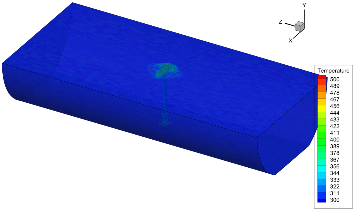
The geometry of interest here is the forward cargo compartment of a Boeing 707. This geometry shortly after a small fire is started in the center can be seen in figure 1(a). The flow is entirely driven by buoyant effects due to the local heating produced by the fire. We note that a short distance away from the fire source, there is no longer a significant effect on the dynamics of the flow due to the actual chemical combustion process taking place. This type of flow can therefore be accurately modeled as a heat source addition into non-reactive air, freeing us from the need to tackle the computationally expensive details of the combustion problem. Experimental results of the full 3D case and background on this problem can be found in work by Oztekin et al[1, 4].

(a) Temperature field after start-up of a small fire in the center.

(b) Flow driven by a heat source in a 2D cross-section. Colormap shown is temperature normalized by the initial bulk temperature.

Figure 1: Example flowfields of buoyancy-driven flow in Boeing 707 cargo hold geometry.

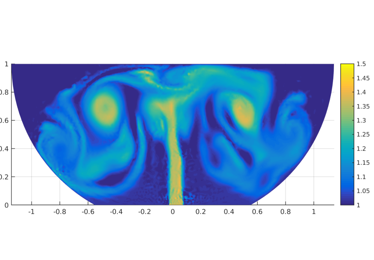
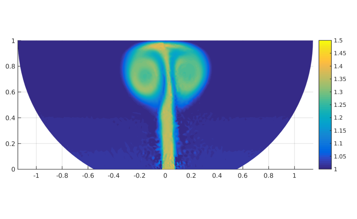
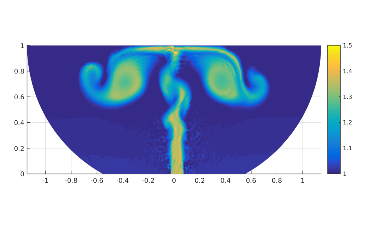
A typical simulation of a 2D cross-section of the cargo geometry (computed using our in-house DG code) can be seen in figure 1(b). A turbulent plume rising from the heat sources drives vortical flow around the compartment feeding back into itself at the bottom. We note recirculation regions in both upper corners leading to stagnation regions where streamlines are separating, indicating a sensor position there would be less effective than at other locations. The turbulent, buoyant flow is instantaneously asymmetric, but statistically averaged is largely symmetric due to symmetric boundary conditions. The base of the geometry is $1.107m$ wide, and the ceiling is $2.286m$ wide and $1m$ tall.

In this work, we restrict the analysis to a 2D cross-section of a cargo hold. All boundary conditions are isothermal, with the majority of the wall boundary fixed to the initial bulk temperature non-dimensionalized to $T_{\infty}=1$. A $0.1m$ wide section of the floor is then set to an isothermal condition at a multiple of the bulk temperature in order to model a heat source. The temperature source $T_{s}$ is examined in the range between $T_{s}=1.2$ and $1.5$, and the temperature location $x_{s}$ in the range between $x_{s}=0.0$ (centerline) and $0.503m$ (the rightmost possible location for $0.1m$ wide source.) Due to symmetry, sources need only be placed to one side of the geometry in order to analyze sources at a reflected point along the floor.

All DNS simulations here are performed using cubic ($N=3$) elements, with the 2D meshes consisting of approximately $1500$ triangular cells. This results in $10$ nodes per cell for each of the $4$ quantities (density, $x$ and $y$ momentum, and energy) to be solved, for a total of $\sim 60,000$ degress of freedom.

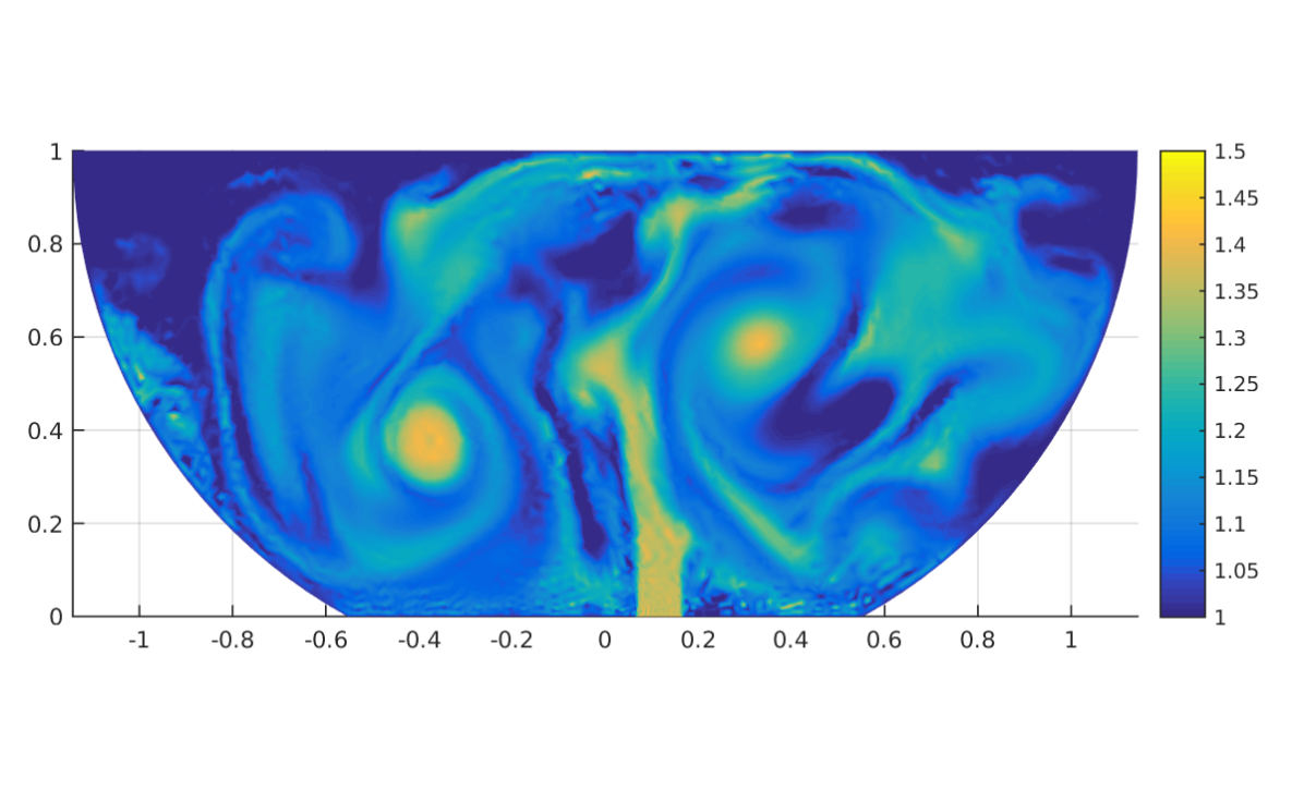
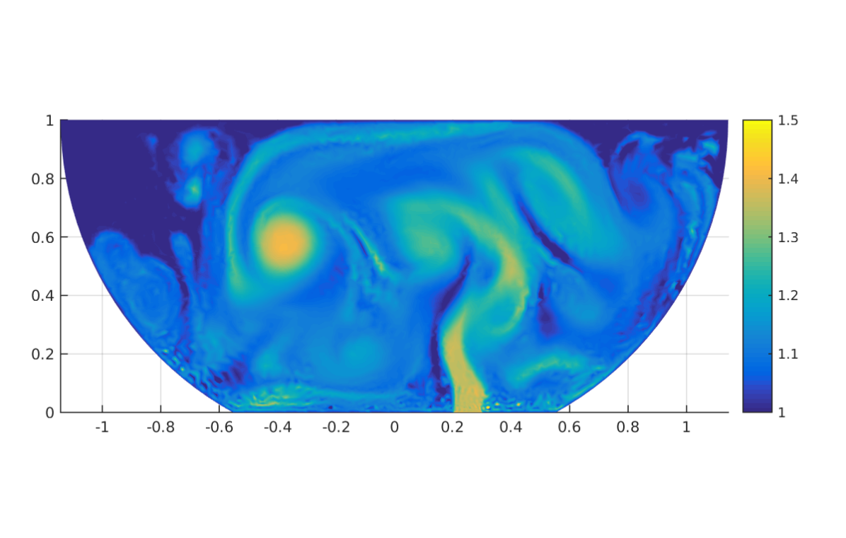
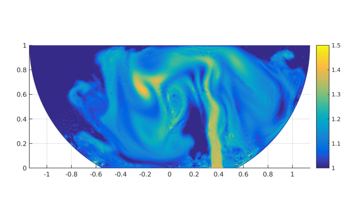
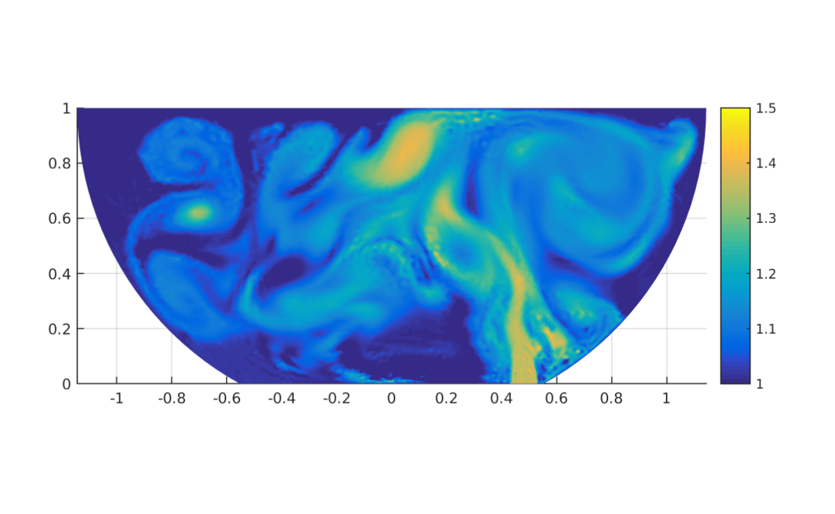
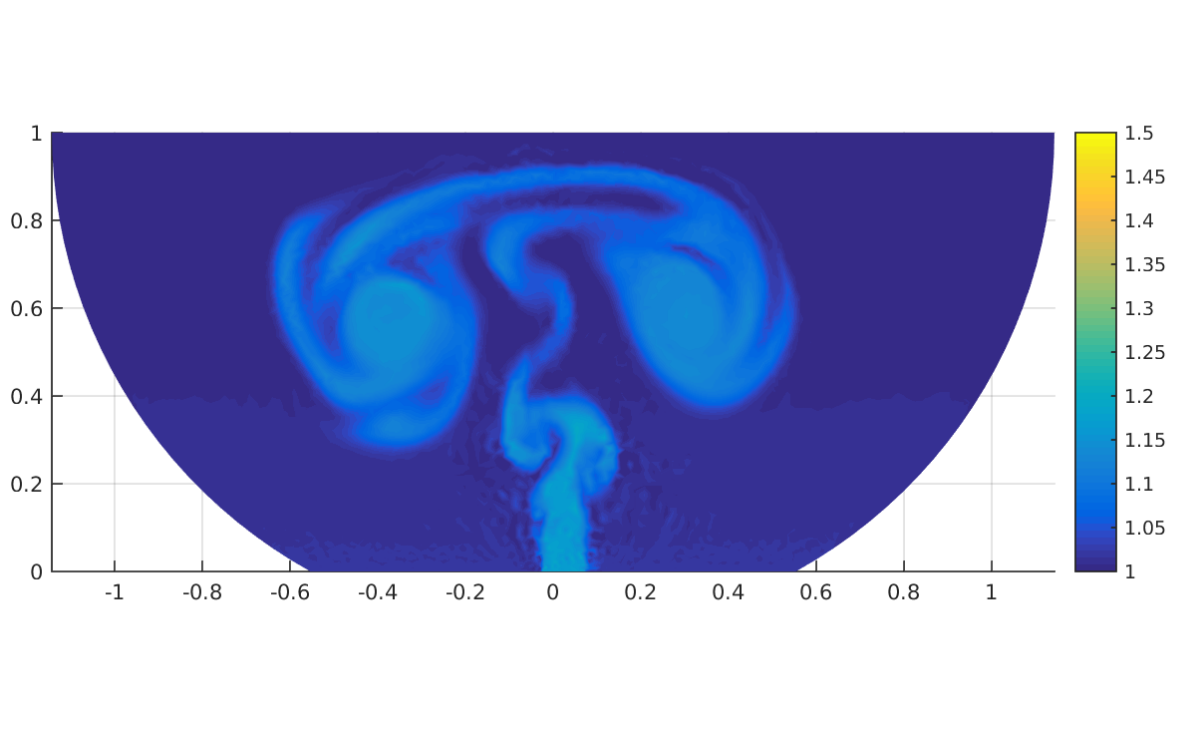
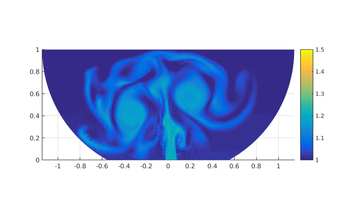
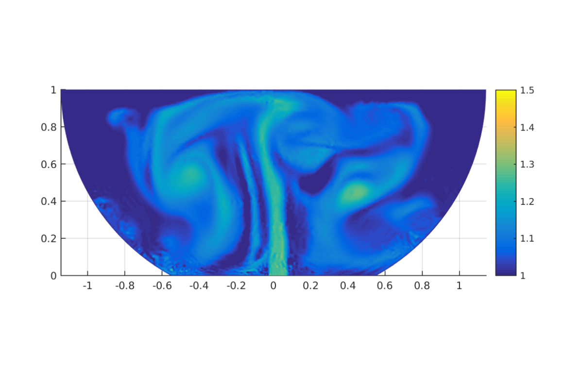
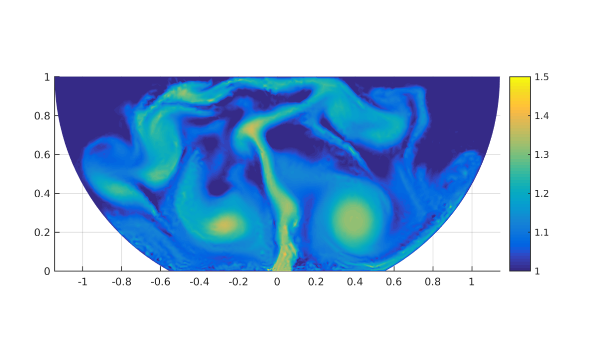
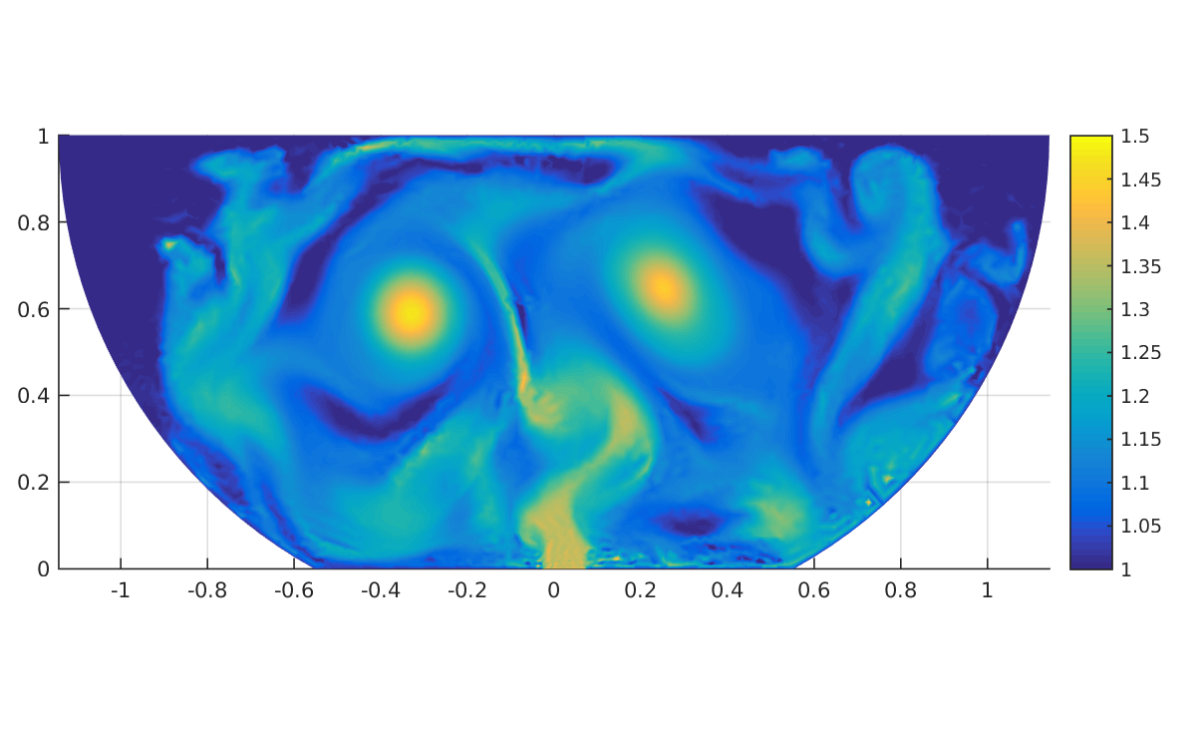
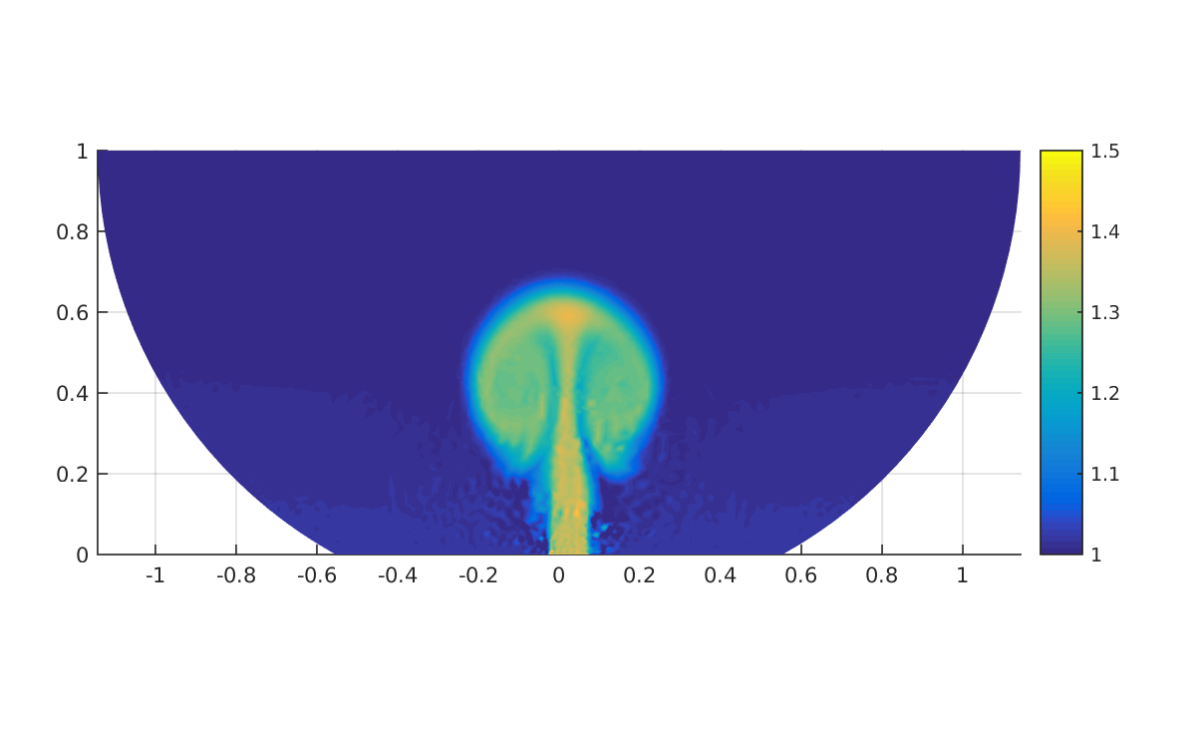
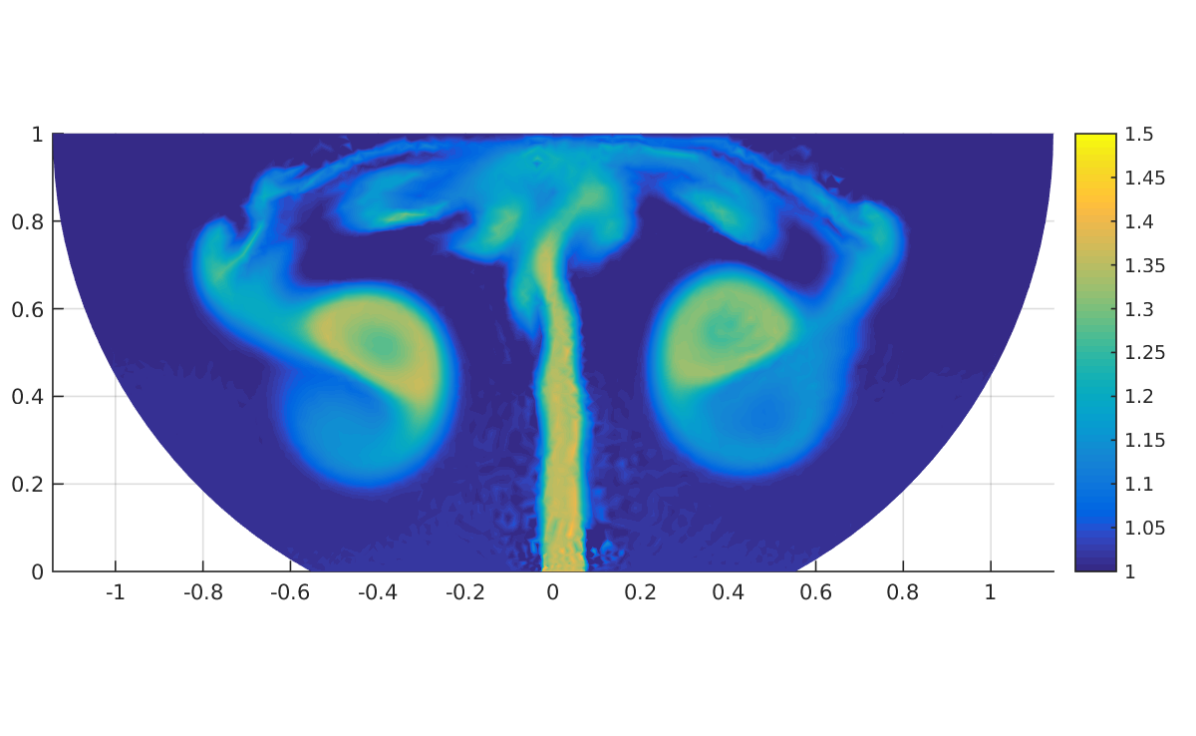
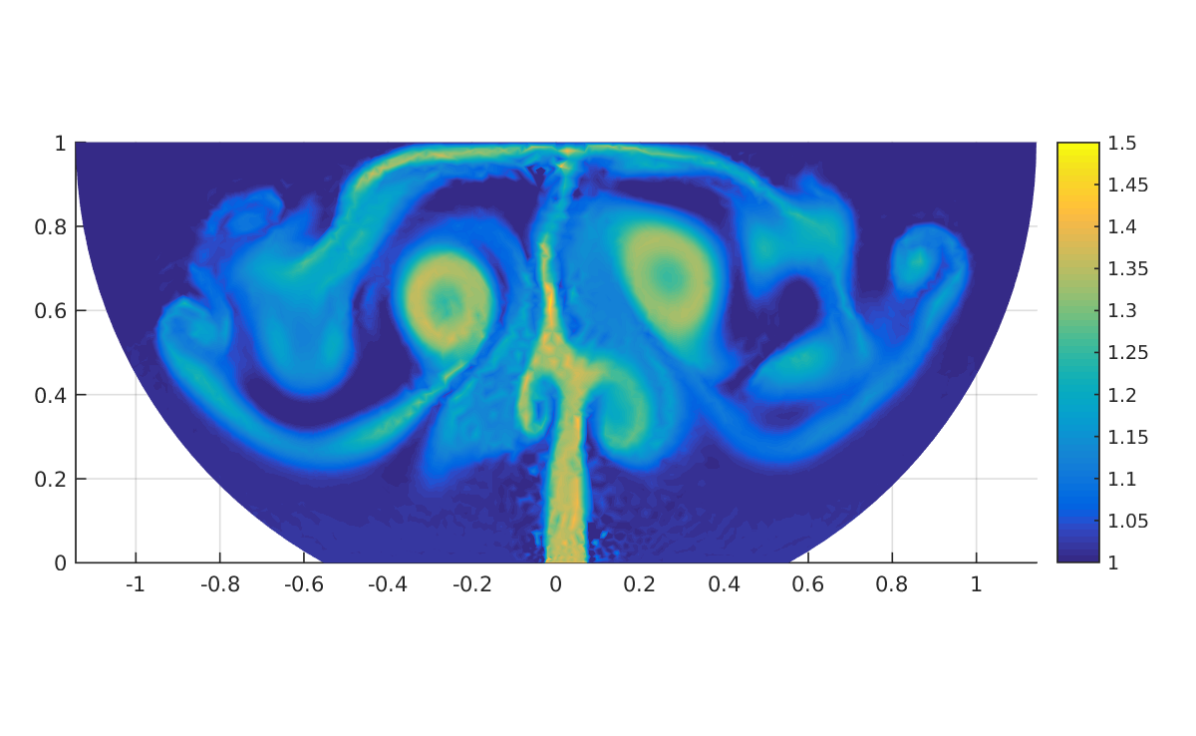
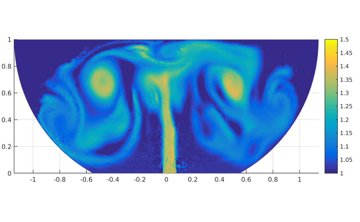
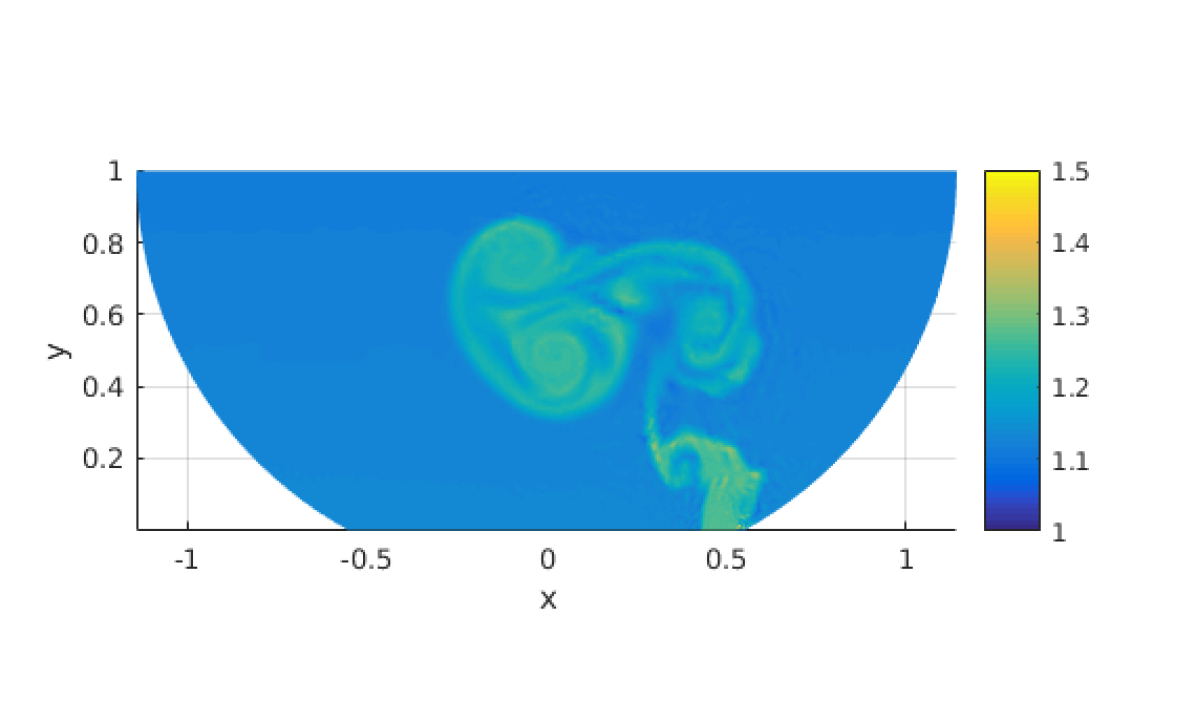
Sample flowfield snapshots of temperature are displayed in Figures 2, 3, and 4. These figures illustrate the wide range of spatio-temporal flow behaviors that are possible when the fire source location and temperature are varied, and motivates a study aimed at quantifying the statistics of some measure of the flow given parameterized uncertainty in the fire source location and temperature.

(a) $x_{s}=0.024m$.

(b) $x_{s}=0.116m$.

(c) $x_{s}=0.262m$.

(d) $x_{s}=0.387m$.

(e) $x_{s}=0.480m$.

Figure 2: Temperature fields for $T_{s}=1.486$ source at the 5 source locations, time $t=10s$ after startup.

(a) $T_{s}=1.214$.

(b) $T_{s}=1.269$.

(c) $T_{s}=1.350$.

(d) $T_{s}=1.431$.

(e) $T_{s}=1.486$.

Figure 3: Temperature fields at $x_{s}=0.024m$ for the 5 values of temperature source, time $t=10s$ after startup.

(a) $t=2s$.

(b) $t=3s$.

(c) $t=4s$.

(d) $t=5s$.

(e) $t=6s$.

(f) $t=7s$.

Figure 4: Temperature field time evolution for $T_{s}=1.486$, $x_{s}=0.024$ case.

3 Uncertainty Quantification using Polynomial Chaos Expansions (PCE)

Motivated by the wide range of possible flow patterns displayed in Figures 2, 3, and 4, our goal is to vary the fire source location $x_{S}$ and temperature $T_{S}$ at the base of the cargo hold and quantify how this affects the flow dynamics, while using a minimal number of DG simulations. We wish to construct a surrogate model that explicitly describes this input-output behavior, which can be inexpensively sampled and analyzed for statistical correlations and trends. As a result of these requirements, we choose to use Polynomial Chaos Expansions (PCE) as our framework for performing UQ.

We give a brief overview of this approach below; further details can be found in introductory references on PCE methods[5, 6, 7].

Let $Z=(Z_{1},Z_{2})$ be a vector of standard random variables that parameterizes the uncertainty in the cargo hold fire simulations. Let $d=2$ be the number of random parameters. We are interested in the corresponding uncertainty of some measure of the fluid dynamics, represented by $y(Z)$. In our setting, $Z_{1}$ is a coordinate that parameterizes the fire source location along the base of the cargo hold, and $Z_{2}$ is a coordinate that parameterizes the fire source temperature. The output, $y(Z)$, is some measure of the fire dynamics; for example, the temperature at specific locations along the ceiling of the cargo hold, at different sample times.

The goal of the method is to represent $y(Z)$ in terms of some basis functions $\Phi_{i}$. Assuming (for ease of exposition) that $y(Z)$ is scalar-valued, we write:

$$y(Z)=\sum_{|i|=0}^{N}y_{i}\Phi_{i}(Z).$$ (8)

Here, $i=(i_{1},i_{2})$ is a multi-index, and $|i|=i_{1}+i_{2}$. We define an inner product on the space of functions of the random variables by

$$\left\langle f,g\right\rangle=\int_{\Gamma}f(Z)g(Z)\rho(Z)\,dZ,$$ (9)

where $\rho(Z)$ denotes the probability density function of $Z$, and has support $\Gamma$. A fundamental insight in PCE methods is to employ basis functions that are orthonormal with respect to this inner product, so that

$$\left\langle\Phi_{i},\Phi_{j}\right\rangle=\delta_{ij},$$ (10)

where $\delta_{ij}=1$ if $i=j$, and $0$ if $i\neq j$. In particular, a multivariate basis polynomial $\Phi_{i}$ may be written as

$$\Phi_{i}(Z)=\prod_{k=1}^{d}\phi_{i_{k}}(Z_{k}),$$ (11)

where $\phi_{n}$ is a (univariate) polynomial of degree $n$. The $\{\phi_{n}\}$ will be a basis of orthogonal polynomials chosen so that the orthogonality condition (10) is satisfied. For example, if we work with uniformly distributed random variables, then our basis polynomials would be the multivariate Legendre polynomials.

The coefficients $y_{i}$ in the expansion (8) may be determined by taking an inner product with $\Phi_{j}$: because the $\Phi_{j}$ are orthonormal, we have

$$y_{j}=\left\langle y,\Phi_{j}\right\rangle.$$ (12)

Note that one could also take $y(Z)$ to be a vector of several different aerodynamic quantities of interest: in this case, the coefficients $y_{i}$ in the expansion (8) are vectors, and each component of $y_{i}$ is determined by an equation such as (12), for the corresponding component of $y$.

The important issue now is how we choose to approximate the projection integrals in (12). A possible choice is to use Gauss quadrature, in which the function $y(Z)$ is evaluated on a grid consisting of the tensor product of $d$ separate 1-D quadrature point sets in parameter space. A drawback of this method is that it suffers from the curse of dimensionality; however, since our uncertain parameter space is only two-dimensional, we choose to use this method.

After computing the PCE surrogate, statistical quantities of interest readily follow. The probability density function of the output quantities may be approximated by Monte Carlo sampling of the PC expansion. The mean $\mu$ and variance $\sigma^{2}$ of the PC model may be analytically computed as a function of the model coefficients:

$$\mu =y_{0}$$ (13)

$$\sigma^{2} =\sum_{|i|=1}^{N}y_{i}^{2}\|\phi_{i}\|^{2}$$

Sobol indices, which provide a metric of the relative “importance” of each of the uncertain parameters on the output, may also be analytically computed from the PC model coefficients [8]. Specifically, the “total” Sobol index $T_{i}$ is defined as the fraction of the total variance contributed by all those polynomials in the PC expansion which involve $Z_{i}$:

$$T_{i} =\frac{\mathbb{E}[\operatorname{Var}(y|Z_{-i})]}{\operatorname{Var}(y)},\qquad i=1,\ldots,d$$ (14)

$$=\frac{1}{\sigma^{2}}\sum_{j}y_{j}^{2}\|\phi_{j}\|^{2}$$

where $j$ in the above expression is understood to index only those terms in the PC expansion which involve parameter $Z_{i}$, $Z_{-i}$ denotes all parameters except $Z_{i}$, and $\mathbb{E}[\cdot]$ denotes the expected value.

4 Case Study: 2-D Cargo Hold Fire with Uncertain Location/Temperature

In this section, we apply the tools discussed to study a test problem in which both the fire source location and temperature are independent, uncertain parameters with some joint probability distribution $\rho(Z)$. We choose to equip both parameters with a uniform distribution. We assume that the range of possible fire source locations consists of the right half of the cargo hold floor. This is done in order to study the effect of spatial asymmetry on the UQ problem. We assume that the range of possible fire source temperatures is given by the interval $[1.2,1.5]\times T_{\infty}$.

Given that both of our parameters are uniformly distributed, our PC basis consists of the Legendre polynomials. We choose to truncate the PC expansion (8) at total order $N=4$. This implies that we use a $5\times 5$ grid of collocation points in the parameter space to evaluate the projection integrals (12), corresponding to the tensor product of the five zeros of the fifth order Legendre polynomials (suitably shifted/scaled) with themselves. These nodes are given in Table 1. These are the collocation points that specify the fire source locations/temperatures that we will simulate using our DG code.

Temperature strength $T_{s}$, $5\times 5$	$1.214,\ 1.269,\ 1.350,\ 1.431,\ 1.486$
Temperature location $x_{s}(m)$, $5\times 5$	$0.024,\ 0.116,\ 0.252,\ 0.387,\ 0.480$

Table 1: Discrete simulation parameters for uncertainty quantification study. The parameter sweep is performed using a tensor product of these values.

Quantifying an entire field quantity $u(x,t;Z)$ using PCE is difficult. This is because the spatio-temporal behavior of the flow can vary significantly with fire source location and temperature, which makes it difficult to interpolate in parameter space accurately using $4^{th}$ order polynomials. Therefore, we focus on a set of observables more amenable to our techniques, corresponding to the temperature along a 1-D segment near the cargo hold ceiling. This observable vector is highly relevant from an engineering standpoint, since it informs the choice of fire sensor placement.

We denote the temperature along the line segment at height $y=0.95$ in the cargo hold as $T_{C}(x,t;Z)$. Intuitively, one would expect a certain characteristic rise time $t_{R}(Z)$ of the buoyant plume from the fire source, which should be dominated by the source temperature (and possibly affected by source location if the plume interacts with the cargo walls). We define $t_{R}(Z)$ as the time required from the start of the fire to detection at any point on the ceiling. For early fire detection, we are interested in the ceiling temperature distribution averaged over a short period of time beginning at $t_{R}(Z)$ (for some choice of $Z$). Therefore, we define the time-averaged ceiling temperature distribution:

$$\overline{T_{C}}(x;Z)=\frac{1}{\Delta t}\int_{t_{R}(Z)}^{t_{R}(Z)+\Delta t}T_{C}(x,t;Z)\;dt\quad,$$ (15)

and we quantify uncertainty in the observables $\overline{T_{C}}(x;Z)$ and $t_{R}(Z)$. We use an averaging time period of $\Delta t=1s$. Note that $t_{R}(Z)$ is a scalar quantity and hence has one PC expansion associated with it, whereas $\overline{T_{C}}(x;Z)$ is a function in $x$ (which is discretized as a vector at discrete locations) and hence has one PC expansion for each location in $x$ we choose to measure. The units of $t_{R}(Z)$ will be seconds; as noted previously, $\overline{T_{C}}(x;Z)$ is temperature normalized by the initial bulk temperature $T_{\infty}$.

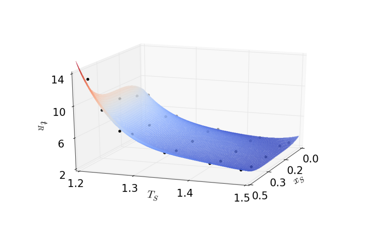
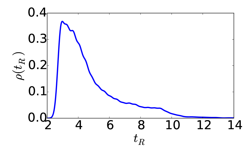
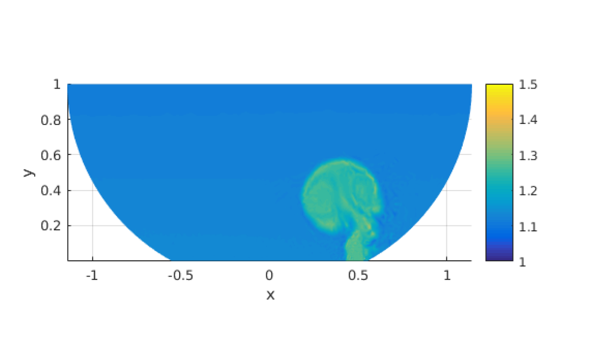
We first examine the rise time $t_{R}(Z)$. The PCE surrogate model for rise times $t_{R}(Z)$ is shown in Figure 5, along with statistical quantities in Table 2. Examination of Figure 5 and Table 2 confirms our hypothesis that the characteristic rise time $t_{R}$ is dominated by the source temperature. As shown, source temperature has a Sobol index of 0.95, which means that $95\%$ of the variance in the distribution of $t_{R}$ can be attributed to source temperature (either acting alone or interacting with location). The only portion of parameter space that really is affected strongly by source location appears to be the “corner” area of parameter space where the source is very close to the cargo hold wall and the source temperature is very low. The result of this combination of variables is that the initial buoyant plume “rolls over” toward the center of the cargo hold and falls back downward toward the floor before reaching a height of $y=0.95$ (where we are observing ceiling temperature). This time-dependent behavior is illustrated in Figure 6. It is not until several seconds after this has occured that subsequent buoyant plumes finally touch the ceiling. This combination of low temperature with a wall effect is what accounts for the tail of the distribution of $t_{R}$.

(a) PCE surrogate map of $t_{R}(Z)$, together with the values at the 25 quadrature nodes.

(b) Probability density function $\rho(t_{R}(Z))$ (approximated using 10,000 random samples of the PCE surrogate).

Figure 5: PCE surrogate for $t_{R}(Z)$.

(a) $t=6s$.

(b) $t=8s$.

(c) $t=10s$.

Figure 6: Temperature field snapshots with $Z=(0.48,1.21)$. The initial plume falls toward the floor without ever touching the ceiling, explaining the unusually long rise time.

Mean	4.8
Variance	3.9
Sobol Index 1 (Location)	0.08
Sobol Index 2 (Temperature)	0.95

Table 2: Statistical quantities of interest for $t_{R}(Z)$.

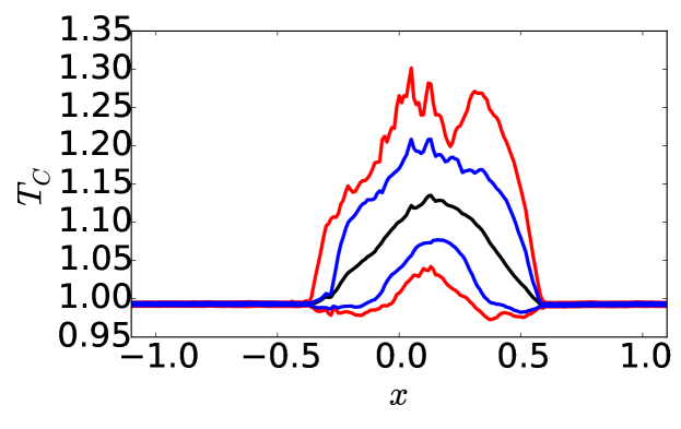
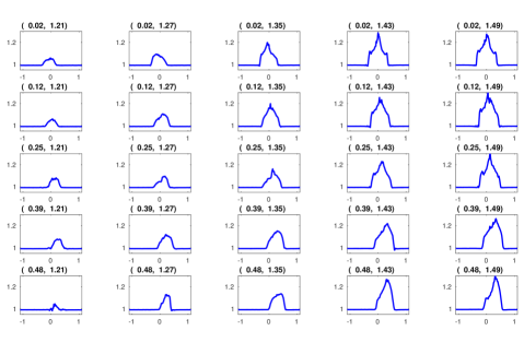
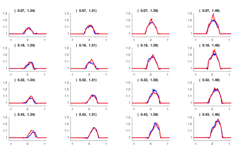
We next turn our attention to the time-averaged ceiling temperature distribution $\overline{T_{C}}(x;Z)$. The time-averaged ceiling temperature distributions at the quadrature nodes are shown in Figure 9. The mean distribution along with confidence intervals – computed from Monte Carlo samples of the PCE surrogate – is shown in Figure 7(a). The accuracy of the PC model for ceiling temperature can be verified by comparing the PC interpolation to data at various points in parameter space. This is done in Figure 10, which confirms that our the PC model provides reasonably accurate interpolation.

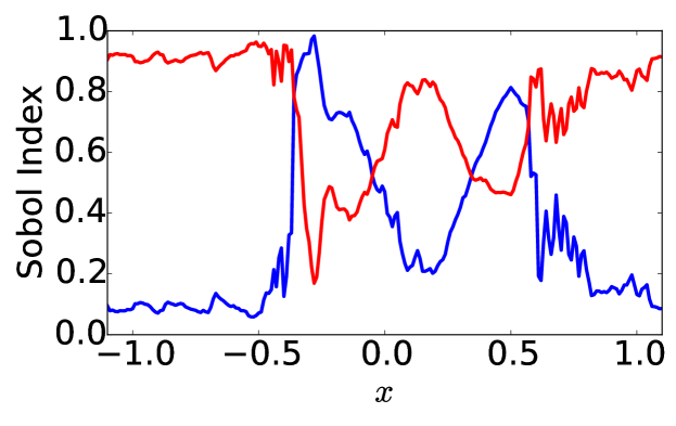
We can also examine the total Sobol indices as a function of $x$ for the ceiling temperature observable, which indicate which of the two uncertain parameters best explains the variance in the ceiling temperature. These Sobol indices are displayed in Figure 7(b). As can be seen, source temperature is the dominant parameter in the area around the maximum of the mean profile. The peripheral areas are dominated by source location. The explanation of this phenomenon is natural: source temperature controls the intensity of the temperature fluctuations observed on the ceiling where they are hottest, but source location determines whether or not temperature fluctuations are actually observed at all in the peripheral areas.

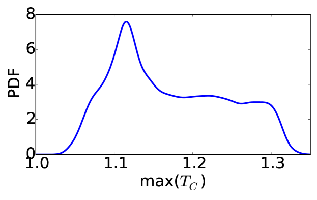
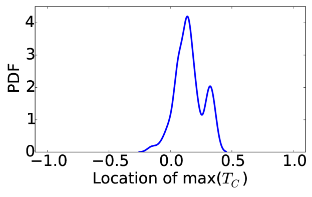
Having a PCE surrogate for ceiling temperature also means that we can compute the statistics of any quantity derived from it. Two particularly relevant examples of this include the maximum value of $\overline{T_{C}}(x;Z)$ as well as its location along the ceiling. We display these statistics in Figure 8. We see that a wide range of maximum ceiling temperatures are possible, with a skew toward lower maximum values. We also see a clear skew in the location of the maximum ceiling temperature to the right of the center (as would be expected from the asymmetry in the source location). Computing correlations between these output quantities and our uncertain parameters confirms what one would expect – source temperature dominates the maximum value of the ceiling temperature, whereas source location dominates its location.

(a) Black: mean time-averaged ceiling temperature profile. Blue: 68$\%$ confidence interval. Red: 95$\%$ confidence interval.

(b) Sobol indices for ceiling temperature at points along the ceiling. Blue: source location. Red: source temperature.

Figure 7: Statistical quantities of interest for time-averaged ceiling temperature.

(a) Distribution of the maximum value of the time-averaged ceiling temperature.

(b) Distribution of the location of the maximum value of the time-averaged ceiling temperature.

Figure 8: Distributions of maximum ceiling temperature value and location. Computed from 10,000 Monte Carlo samples of the PCE surrogate.

Figure 9: Time-averaged ceiling temperature distributions collected at the 25 quadrature nodes. Each subtitle corresponds to the parameter pair $(x_{S},T_{S})$.

Figure 10: Time-averaged ceiling temperature distributions collected at points on the 4x4 mesh which is dual to the 5x5 mesh. Data are displayed in blue; PC models are displayed in red. Each subtitle corresponds to the parameter pair $(x_{S},T_{S})$.

Combining all of this information together gives a clear and insightful view of the physics of our cargo hold problem. We see that the main effects of increasing temperature are to increase the maximum ceiling temperature, and to decrease the rise time. The main effect of location is to influence whether or not fluctuations in ceiling temperature are observed in the peripheral regions of the ceiling. The fact that we observe these intuitive trends in our surrogate model gives us further validation of the claim that PCE methods may provide a method for UQ which is not only efficient, but also accurate for this class of problems.

Of course, the main usage of these UQ tools is not just to confirm intuition, but to quantify it. We see that, on average, we can expect a ceiling temperature distribution which is roughly symmetric between the limits $y\in[-0.35,0.60]$, with a maximum around $y=0.125$. We can also give confidence intervals on the mean ceiling temperature distribution (Figure 7), and estimate the probability distributions for the value and location of the maximum ceiling temperature (Figure 8).

5 Conclusions

The purpose of this paper was establish a framework for performing efficient, accurate investigations of the statistical variations in cargo hold fires that occur due to parameterized uncertainty in the boundary conditions. We address two related problems – increasing the numerical accuracy of the CFD simulation, and uncertainty quantification. Higher order numerical accuracy is necessary because traditional finite-volume schemes require a prohibitively fine mesh in order to resolve the vortex-dominated flows seen in cargo hold fire solutions. The need for uncertainty quantification stems from the fact that the boundary conditions of the cargo hold fire will always be fundamentally unpredictable, since one can never know a priori exactly where the fire will start, how hot it will be, how much luggage clutter there is, etc.

In order to provide greater simulation accuracy, we developed an in-house discontinuous Galerkin (DG) flow solver for the compressible Navier-Stokes equations with buoyancy effects. This code also features an unstructured mesh suitable for complex geometries. To make uncertainty quantification feasible, we first reduced the problem from quantifying the full flow field to quantifying measures of the flow field – a characteristic rise time of the buoyant flow, and a time-averaged ceiling temperature distribution. This made the problem amenable to treatment with spectral expansion methods, and so we used PCE as the tool to efficiently and accurately quantify the effects of fire source location and temperature. A case study of a 2D cargo hold geometry in which the fire source location and temperature were uncertain confirmed that PCE tools provide a viable UQ approach, and keep the number of required CFD simulations to a minimum.

We are currently working to extend these methods to 3D cargo hold fire configurations. We are also planning to investigate methods for accounting for geometric uncertainty in cargo hold luggage clutter, which was not accounted for in our empty cargo hold geometries.

6 Acknowledgments

This research was supported under the Federal Aviation Administration (FAA) Joint University Program (JUP). The authors would also like to thank Ezgi Oztekin for helpful discussions on previous cargo hold fire research as well as a tour of the cargo hold fire testing facilities at the FAA Tech Center.

References

- [1] Oztekin, E. S., “Heat and mass transfer due to a small-fire in an aircraft cargo compartment,” International Journal of Heat and Mass Transfer, Vol. 73, 2014, pp. 562–573.
- [2] Hesthaven, J. and Warburton, T., Nodal Discontinuous Galerkin Methods: Algorithms, Analysis, and Applications, Texts in Applied Mathematics, Springer, 2008.
- [3] Knoll, D. and Keyes, D., “Jacobian-free Newton–Krylov methods: a survey of approaches and applications,” Journal of Computational Physics, Vol. 193, No. 2, jan 2004, pp. 357–397.
- [4] Oztekin, E. S., Zha, G.-c., and Lyon, R. E., “Flow induced by a small fire in an aircraft cargo compartment,” 50th AIAA Aerospace Sciences Meeting, No. January, Nashville, TN, 2012.
- [5] Ghanem, R. G. and Spanos, P., Stochastic Finite Elements: A Spectral Approach, Springer-Verlag, New York, 1991.
- [6] Xiu, D., Numerical Methods for Stochastic Computations: A Spectral Method Approach, Princeton University Press, 2010.
- [7] LeMaitre, O., Spectral Methods for Uncertainty Quantification, Springer, 2010.
- [8] Sudret, B., “Global sensitivity analysis using polynomial chaos expansion,” Reliability Engineering and System Safety, 2007.