Globally Optimal Joint Uplink Base Station Association and Beamforming*

Abstract

The joint base station (BS) association and beamforming problem has been studied extensively in recent years, yet the computational complexity for even the simplest SISO case has not been fully characterized. In this paper, we consider the problems for an uplink SISO/SIMO cellular network under the max-min fairness criterion. We first prove that the problems for both the SISO and SIMO scenarios are polynomial time solvable. Secondly, we present a fixed point based binary search (BS-FP) algorithm for both SISO and SIMO scenarios whereby a QoS (Quality of Service) constrained subproblem is solved at each step by a fixed point method. Thirdly, we propose a normalized fixed point (NFP) iterative algorithm to directly solve the original problem and prove its geometric convergence to global optima. Although it is not known whether the NFP algorithm is a polynomial time algorithm, empirically it converges to the global optima orders of magnitude faster than the polynomial time algorithms, making it suitable for applications in huge-scale networks.

I Introduction

To meet the surging mobile traffic demand, wireless cellular networks have increasingly relied on low power transmit nodes such as pico base stations (BS) to work in concert with the existing macro BSs. Such a heterogeneous network (HetNet) architecture can provide substantially improved data service to cell edge users.

One crucial problem in the system design of future networks is how to associate mobile users with serving BSs. The conventional greedy scheme that associates receivers with the transmitter providing the strongest signal and its modern variant Range Extension [2] may be suboptimal during periods of congestion. A more systematic approach is to jointly design BS association and other system parameters so as to maximize a network-wide utility. The early work in this direction [3] and [4] proposed a fixed point iteration to jointly adjust BS association and power allocation in the uplink (UL), while subject to QoS (Quality of Service) constraints, with the goal to minimize total transmit power. The global convergence of this algorithm has been established when the problem is feasible. This algorithm has been extended to the single input single output (SISO) cellular network with power budget constraints for both the UL and the downlink (DL) in [5, 6], respectively. The fixed point algorithm in [3, 4] can also be interpreted as an alternating optimization approach: fix the BS association, each user updates it power to satisfy the QoS Constraint; fix the power, each user updates its BS association to maximize its SINR (Signal to Interference plus Noise Ratio). This alternating optimization approach was extended to joint BS association, power allocation and beamforming for UL SIMO cellular network in [7].

Recently, various approaches have been applied to tackle the BS association problem [8, 9, 10, 11, 12]. The work in [8] proposed to solve a utility maximization problem by alternately optimizing over BS association and other system parameters for SISO DL cellular network. References [9, 10] considered a partial CoMP (Coordinated Multiple Point) transmission strategy, i.e., allowing one user to be served by multiple BSs for MIMO DL cellular network. They proposed sparse optimization techniques to compute a desirable BS association that incurs low overhead. References [11, 12] studied the joint design of BS association and frequency resource allocation for a fixed transmission power for DL SISO Cellular Network .

The computational complexity of maximizing a certain utility function by joint BS association and power allocation has been studied in different scenarios [13, 14, 15]. For the sum rate utility function, the NP hardness of the joint design problem has been established for both the UL MIMO cellular network [13] and the DL MIMO cellular network [14]. As a counterpart, for the max-min fairness utility, the joint design problem in a DL SISO network is shown to be NP-hard in general, while for some special cases (with an equal number of users and BSs and under additional QoS constraints) this problem is shown to be polynomial time solvable [16].

Despite the extensive research, a fundamental theoretical question remains open: is the joint design problem under max-min fairness criterion in an UL cellular network polynomial time solvable? In addition, to handle large scale networks, fast algorithms with performance guarantee (not only theoretically polynomial time solvable) are much needed.

In this paper, we aim to resolve these issues. In particular, we consider the joint BS association and beamforming problem under the the max-min fairness criterion for both UL SISO and SIMO cellular networks. Our main contributions are as follows:

1. We prove that the problems for both SISO and SIMO scenarios are polynomial time solvable. To be more specific, we show that the problem for SIMO (resp. SISO) networks can be solved by a binary search method whereby each subproblem can be solved by SDP (resp. LP), and we refer to this algorithm as BS-SDP (resp. BS-LP). This is rather surprising since the considered optimization problem involves discrete variables and falls into the class of mixed integer nonlinear programming.

2. We present a globally optimal fixed point based binary search (BS-FP) algorithm in which the QoS constrained subproblems are solved by fixed point algorithms, which can avoid invoking a LP solver for SISO scenarios or a SDP solver for SIMO scenarios.

3. We propose a normalized fixed point (NFP) algorithm to directly solve the joint BS association and beamforming max-min fairness problem, which can avoid binary search. Theoretically, using results from the concave Perron-Frobenius theory [17, 18], we prove the geometric convergence of the proposed algorithm to global optima. At this point, we are only able to show the pseudo-polynomial time, not polynomial time complexity, of the NFP algorithm, although empirically it is much faster than the polynomial time algorithms BS-LP and BS-SDP. In fact, the NFP algorithm converges in less than 20 iterations for networks with hundreds of BSs and users, as shown in the numerical experiments.

We summarize the computational complexity results for the joint BS association and beamforming problem under the max-min fairness criterion for both UL and DL cellular networks in Table I below.

Table I: The Complexity Status of the Joint BS Association and Beamforming Problem (max-min fairness)

	Fixed BS association	Joint
		UL	DL
SISO	Polynomial [19]	Polynomial (Theorem 1)	NP-Hard [16]
SIMO	Polynomial [20]	Polynomial (Theorem 3)	NP-Hard [16]
MISO	Polynomial [21, 22]	Unknown	NP-Hard [16]
MIMO	NP-Hard [23]	Unknown	NP-Hard [16]

This paper is structured as follows. In Section II, the max-min fairness problem by joint BS association, power control and beamforming problem for an UL SIMO cellular network is introduced. In Section III, we investigate the SISO scenario. We first prove the polynomial time solvability for the SISO scenario, then present a BS-FP algorithm and finally propose the NFP algorithm. In Section IV we investigate the SIMO scenario. We first prove the polynomial time solvability for the SIMO scenario, then present a BS-FP algorithm and finally propose the NFP algorithm. Simulation results are provided in Section V to compare the efficiency and the effectiveness of the algorithms. Finally, some concluding remarks are offered in Section VI.

II System Overview

Consider an uplink cellular network where $K$ mobile users transmit to $N$ BSs. Each user is equipped with a single antenna and the $n$th BS is equipped with $M_{n}\geq 1$ antennas, $n=1,\cdots,N$. They share the same time/frequency resource for transmission. Each user is to be associated with exactly one BS, but one BS can serve multiple users. Assuming that the transmitted signal from the $k$th mobile user is $s_{k}$, the received signal $\boldsymbol{y}_{n}$ at the $n$th BS may be expressed as

$$\boldsymbol{y}_{n}=\sum_{k=1}^{K}\boldsymbol{h}_{nk}s_{k}+\boldsymbol{n}_{n},$$ (1)

where the $M_{n}$-dimensional vector $\boldsymbol{h}_{nk}$ denotes the flat fading channel coefficient between the $k$th mobile user and the $n$th BS, while the $M_{n}$-dimensional vector $\boldsymbol{n}_{n}$ denotes the AWGN with zero mean and a covariance matrix of $\sigma_{n}^{2}\boldsymbol{I}$. Let $\bm{a}=(a_{1},a_{2},\dots,a_{K})$ denote the association profile, i.e., $a_{k}=i$ if user $k$ is associated with BS $i$. For the $k$th user, the BS $a_{k}$ invokes a $M$-dimensional unit-norm linear receiver $\boldsymbol{u}_{a_{k},k}$ to generate the decision signal $\tilde{s}_{k}$ for the $k$th user as

$$\tilde{s}_{k} =\boldsymbol{u}_{a_{k},k}^{H}\boldsymbol{y}_{a_{k}}=\boldsymbol{u}_{a_{k},k}^{H}\sum_{j=1}^{K}\boldsymbol{h}_{a_{k},j}s_{j}+\boldsymbol{u}_{i,k}^{H}\boldsymbol{n}_{k}$$

$$=\boldsymbol{u}_{a_{k},k}^{H}\boldsymbol{h}_{a_{k},k}s_{k}+\boldsymbol{u}_{a_{k},k}^{H}\sum_{j=1,j\not=k}^{K}\boldsymbol{h}_{a_{k},j}s_{j}+\boldsymbol{u}_{a_{k},k}^{H}\boldsymbol{n}_{a_{k}}.$$ (2)

The SINR for the $k$th user is given by

$$\textrm{SINR}_{k}=\frac{p_{k}\boldsymbol{u}_{a_{k},k}^{H}\boldsymbol{h}_{a_{k},k}\boldsymbol{h}_{a_{k},k}^{H}\boldsymbol{u}_{a_{k},k}}{\sigma_{a_{k}}^{2}+\boldsymbol{u}_{a_{k},k}^{H}\sum_{j=1,j\not=k}^{K}p_{j}\boldsymbol{h}_{a_{k},j}\boldsymbol{h}_{a_{k},j}^{H}\boldsymbol{u}_{a_{k},k}},$$ (3)

where $p_{k}=E[s_{k}s_{k}^{*}]$ denotes the transmission power of the $k$th user.

$$\begin{split}\textrm{(P)}:\max_{\begin{subarray}{c}\boldsymbol{a},\boldsymbol{p},\\ \{\boldsymbol{u}_{n,k}\}_{\begin{subarray}{c}k=1,\dots,K,\\ n=1,\dots,N\end{subarray}}\end{subarray}}&\min_{k=1,\dots,K}\textrm{SINR}_{k}\\ \textrm{s.t.}\quad&0\leq p_{k}\leq\bar{p}_{k},\;k=1,\dots,K,\\ &a_{k}\in\{1,2,\dots,N\},\;k=1,\dots,K,\\ &\|\boldsymbol{u}_{n,k}\|=1,\;k=1,\dots,K,n=1,\dots,N,\end{split}$$ (4)

where $\bar{p}_{k}$ is the power budget of the $k$th user.

In the following, we will investigate the SISO and SIMO scenarios, respectively. Note that the results and algorithms for SIMO are more general than those for SISO; but to make the ideas easier to understand, we will present those for SISO separately.

III Joint BS Association and Power Control for UL SISO Celluar Networks

In this section, we consider the SISO system where $M_{n}=1,\forall\ n$. In this case, each beamforming vector ${\boldsymbol{u}_{n,k}}$ reduces to a scaler $u_{n,k}$ and the optimal $u_{n,k}$ is given by $\hat{u}_{n,k}=h_{n,k}^{\dagger}/\|h_{n,k}\|$, where the superscript $\dagger$ denotes the complex conjugation. Substituting $\hat{u}_{n,k}$ into problem (P) yileds

$$\begin{split}\textrm{(P\textsubscript{SISO})}:\max_{\bm{p},\bm{a}}&\min_{k=1,\dots,K}{\rm SINR}_{k}=\frac{g_{a_{k}k}p_{k}}{\sigma_{a_{k}}^{2}+\sum_{j\neq k}g_{a_{k}j}p_{j}},\\ \textrm{s.t.}\quad&0\leq p_{k}\leq\bar{p}_{k},\;k=1,\dots,K,\\ &a_{k}\in\{1,2,\dots,N\},\;k=1,\dots,K,\end{split}$$ (5)

where $g_{ik}=\|h_{ik}\|^{2}$ is the channel gain between user $k$ and BS $i$.

Optimizing $\bm{p}$ and $\bm{a}$ separately is easy. Specifically, given a fixed BS association $\bm{a}$, the formulation (5) is a max-min fairness power control problem for an I-MAC (interfering multiple-access channel). It can be solved in polynomial time using a binary search strategy whereby a QoS constrained subproblem is solved by LP (Linear Programming) at each step [19]. Moreover, notice that the interference for user $k$ is $\sum_{j\neq k}g_{a_{k}j}p_{j}$, which only depends on $a_{k}$, and does not depend on $a_{j},\forall j\neq k$. Thus, given a power vector $\bm{p}$, the optimal association of each user $k$ does not depend on the choices of other users and can be easily computed:

$$a_{k}=\arg\max_{n\in\{1,\dots,N\}}\left\{\frac{g_{nk}p_{k}}{\sigma_{n}^{2}+\sum_{j\neq k}g_{nj}p_{j}}\right\}.$$ (6)

In case of multiple $n$’s that achieve the maximum in (6), we just use $\arg\max\{\dots\}$ to represent any element achieving the maximum. However, it is not straightforward to jointly optimize the continuous variable $\bm{p}$ and the discrete variable $\bm{a}$, and this is the focus of our work.

III-A Polynomial Time Solvability

In this section, we will prove that the problem (P_SISO) is polynomial time solvable.

Theorem 1

The problem (P_SISO), i.e., maximizing the minimum SINR by joint BS association and power control for an uplink SISO cellular network, is polynomial time solvable.

Proof:

The max-min fairness problem is closely related to the QoS constrained problem, i.e., minimize the total transmission power subject to the QoS constraints. The QoS constrained joint BS association and power allocation problem is given as follows:

$$\textrm{(P\textsubscript{SISO-QoS})}:\min_{\boldsymbol{p},\boldsymbol{a}} \sum_{k=1}^{K}p_{k},$$

s.t. $$0\leq p_{k}\leq\bar{p}_{k},\;k=1,\dots,K,$$ (7a)

$$a_{k}\in\{1,2,\dots,N\},\;k=1,\dots,K,$$ (7b)

$${\rm SINR}_{k}=\frac{g_{a_{k}k}p_{k}}{\sigma_{a_{k}}^{2}+\sum_{j\neq k}g_{a_{k}j}p_{j}}\geq\gamma,\;$$ (7c)

$$k=1,\dots,K,$$

where $\gamma$ is the required SINR value. Thus, problem (P_SISO) can be solved by a sequence of subproblems of the form (P_SISO-QoS) and a binary search on $\gamma$. In the following, we will show that the QoS constrained subproblem (P_SISO-QoS) can be transformed to a linear programming (LP).

Since the optimal BS association $a_{k}$ is given by (6), we have

$$\exists\ \boldsymbol{a}\leavevmode\nobreak\ \leavevmode\nobreak\ \textrm{satisfying}\leavevmode\nobreak\ \leavevmode\nobreak\ \textrm{(\ref{min power_SISO_2}) and (\ref{min power_SISO_3})}$$

$$\Longleftrightarrow\max_{n\in\{1,\dots,N\}}\frac{g_{nk}p_{k}}{\sigma_{n}^{2}+\sum_{j\not=k}g_{nj}p_{j}}\geq\gamma,\ k=1,\dots,K$$ (8)

$$\Longleftrightarrow p_{k}\geq\min_{n\in\{1,\dots,N\}}\gamma(\boldsymbol{g}_{k}^{n}\boldsymbol{p}+\tilde{\sigma}_{nk}^{2}),\ k=1,\dots,K,$$ (9)

where $\boldsymbol{g}_{k}^{n}=[g_{n1}/g_{nk},\cdots,g_{n(k-1)}/g_{nk},0,g_{n(k+1)}/g_{nk},\cdots,$ $g_{nK}/g_{nk}]$ and $\tilde{\sigma}_{nk}^{2}=\sigma_{n}^{2}/g_{nk}$. Consequently, the problem (P_SISO-QoS) is equivalent to the following problem:

$$\begin{split}\textrm{(P\textsubscript{SISO-QoS-1})}:\min_{\boldsymbol{p}}&\sum_{k=1}^{K}p_{k},\\ \textrm{s.t.}\quad&0\leq p_{k}\leq\bar{p}_{k},\;k=1,\dots,K,\\ &p_{k}\geq\min_{n}\gamma(\boldsymbol{g}_{k}^{n}\boldsymbol{p}+\tilde{\sigma}_{n}^{2}),\;k=1,\dots,K.\end{split}$$ (10)

According to [4, Lemma 4(2)], the equation

$$p_{k}=\min_{n}\gamma(\boldsymbol{g}_{k}^{n}\boldsymbol{p}+\tilde{\sigma}_{n}^{2}).$$ (11)

has a unique fixed point, denoted as $\hat{\bm{p}}$.

Let us consider another QoS constrained problem (P_SISO-QoS-2) below:

$$\begin{split}\textrm{(P\textsubscript{SISO-QoS-2})}:\max_{\boldsymbol{p}}&\sum_{k=1}^{K}p_{k},\\ \textrm{s.t.}\quad&0\leq p_{k}\leq\bar{p}_{k},\ k=1,\dots,K;\\ &p_{k}\leq\min_{n}\gamma(\boldsymbol{g}_{k}^{n}\boldsymbol{p}+\tilde{\sigma}_{n}^{2}),\;k=1,\dots,K.\end{split}$$ (12)

This problem is always feasible since $(0,0,\dots,0)$ is one feasible solution; in addition, the objective value is upper bounded by $\sum_{k}\bar{p}_{k}$, thus the optimal solution to (P_SISO-QoS-2) always exists.

The following result shows that (P_SISO-QoS-1) and (P_SISO-QoS-2) are “equivalent”.

Lemma 1

The two problems (P_SISO-QoS-1) and (P_SISO-QoS-2) are equivalent in the following sense: if (P_SISO-QoS-1) is infeasible, then for any optimal solution to (P_SISO-QoS-2), denoted as $\tilde{\bm{p}}$, there exists some $k$ such that $\tilde{p}_{k}<\min_{n}\gamma(\bm{g}_{k}^{n}\tilde{\bm{p}}+\tilde{\sigma}^{2}_{n})$; if (P_SISO-QoS-1) is feasible, then $\hat{\bm{p}}$ is the unique optimal solution to both (P_SISO-QoS-1) and (P_SISO-QoS-2), where $\hat{\bm{p}}$ is the unique fixed point of (11).

Proof: If (P_SISO-QoS-1) is infeasible, suppose $\tilde{\bm{p}}$ is one optimal solution to (P_SISO-QoS-2), then $\tilde{p}_{k}\leq\min_{n}\gamma(\bm{g}_{k}^{n}\tilde{\bm{p}}+\tilde{\sigma}^{2}_{n}),\forall k$. We must have $\tilde{p}_{k}<\min_{n}\gamma(\bm{g}_{k}^{n}\tilde{\bm{p}}+\tilde{\sigma}^{2}_{n})$ for some $k$; otherwise $\tilde{p}_{k}=\min_{n}\gamma(\bm{g}_{k}^{n}\tilde{\bm{p}}+\tilde{\sigma}^{2}_{n}),\forall k$, implying that $\tilde{\bm{p}}$ is a feasible solution to (P_SISO-QoS-1), a contradiction.

If (P_SISO-QoS-1) is feasible, we claim that its optimal solution $\bm{p}^{*}$ must satisfy (11). In fact, if one $p_{k}^{*}>\min_{n}\gamma(\boldsymbol{g}_{k}^{n}\boldsymbol{p}^{*}+\tilde{\sigma}_{n}^{2})$, then we can reduce the power $p_{k}^{*}$ to strictly improve the objective function without violating all constraints. According to [4, Lemma 4 (2)], the solution to the fixed point equation (11) is unique. Thus $\bm{p}^{*}$ must coincide with $\hat{\bm{p}}$ and (P_SISO-QoS-1) has a unique optimal solution $\hat{\bm{p}}$.

Next, we show that $\hat{\bm{p}}$ is also the unique optimal solution to (P_SISO-QoS-2). Assume the contrary, that (P_SISO-QoS-2) has an optimal solution $\tilde{\bm{p}}\neq\hat{\bm{p}}$. Due to the optimality of $\tilde{\bm{p}}$, we have

$$\sum_{k}\tilde{p}_{k}\geq\sum_{k}\hat{p}_{k}.$$ (13)

Define a set $\mathcal{K}=\{k\mid\tilde{p}_{k}>\hat{p}_{k}\}$. According to (13) and the assumption $\tilde{\bm{p}}\neq\hat{\bm{p}}$, the set $\mathcal{K}$ must be nonempty; otherwise, we have $\tilde{p}_{k}\leq\hat{p}_{k},\forall k$, which together with (13) implies $\tilde{p}_{k}=\hat{p}_{k}$, a contradiction.

Define $k_{0}=\arg\max_{k}\left\{\frac{\tilde{p}_{k}}{\hat{p}_{k}}\right\}$ and $\tau=\max_{k}\left\{\frac{\tilde{p}_{k}}{\hat{p}_{k}}\right\}=\frac{\tilde{p}_{k_{0}}}{\hat{p}_{k_{0}}}>1$, then

$$\tau\hat{p}_{j}\geq\tilde{p}_{j},\ \forall j.$$ (14)

We have

$$\min_{n}\gamma(\bm{g}_{k_{0}}^{n}\tilde{\bm{p}}+\tilde{\sigma}_{n}^{2})\overset{(i)}{\geq}\tilde{p}_{k_{0}}=\tau\hat{p}_{k_{0}}\overset{(ii)}{=}\tau\gamma\min_{n}(\bm{g}_{k_{0}}^{n}\hat{\bm{p}}+\tilde{\sigma}_{n}^{2})$$

$$\overset{(iii)}{>}\gamma\min_{n}(\bm{g}_{k_{0}}^{n}\tau\hat{\bm{p}}+\tilde{\sigma}_{n}^{2})\overset{(iv)}{\geq}\gamma\min_{n}(\bm{g}_{k_{0}}^{n}\tilde{\bm{p}}+\tilde{\sigma}_{n}^{2}).$$

Here, $(i)$ is because $\bm{\tilde{}}{p}$ satisfies the constraints of (P_SISO-QoS-2), $(ii)$ is because $\hat{\bm{p}}$ is the fixed point of (11), $(iii)$ is due to the facts that $\tau>1$ and the noise variance $\tilde{\sigma}_{n}^{2}>0,\forall n$, and $(iv)$ follows from (14). The above relation is a contradiction, thus $\hat{\bm{p}}$ must be the unique optimal solution to (P_SISO-QoS-2). $\Box$

Lemma 1 implies that solving (P_SISO-QoS-2) either provides an optimal solution to (P_SISO-QoS-1) or provides an infeasibility certificate for (P_SISO-QoS-1); in fact, (P_SISO-QoS-1) is infeasible if and only if for any optimal solution to (P_SISO-QoS-2) there is at least one active inequality. Therefore, Lemma 1 leads to a two-step algorithm for solving (P_SISO-QoS-1):

Step 1: Find one optimal solution $\tilde{\bm{p}}$ to (P_SISO-QoS-2).

Step 2: Equality test: test whether $\tilde{p}_{k}=\min_{n}\gamma(\bm{g}_{k}^{n}\tilde{\bm{p}}+\tilde{\sigma}^{2}_{n}),\forall k$. If yes, then $\tilde{\bm{p}}$ is the unique optimal solution to (P_SISO-QoS-1); if no, then (P_SISO-QoS-1) is infeasible.

Problem (P_SISO-QoS-2) can be recast as

$$\begin{split}\textrm{(P\textsubscript{SISO-QoS-LP})}:\max_{\boldsymbol{p}}&\sum_{k=1}^{K}p_{k},\\ \textrm{s.t.}\quad&0\leq p_{k}\leq\bar{p}_{k},\;k=1,\dots,K,\\ &p_{k}\leq\gamma(\boldsymbol{g}_{k}^{n}\boldsymbol{p}+\tilde{\sigma}_{n}^{2}),\;\\ &k=1,\dots,K,n=1,\dots,N,\end{split}$$ (15)

which is an LP (linear programming) and thus polynomial time solvable. As a result, (P_SISO-QoS-1) can be solved by a two-step algorithm where the first step consists of solving an LP, and the second step is a simple equality test. Thus (P_SISO-QoS-1) can be solved in polynomial time.

Let us come back to the proof of Theorem 1. (P_SISO) can be solved by a binary search method whereby each subproblem (P_SISO-QoS-1) can be solved by an LP plus an equality test (we refer to this method as BS-LP algorithm), thus (P_SISO) is polynomial time solvable. ∎

III-B A Fixed Point Based Binary Search Algorithm

In the BS-LP algorithm, we need to solve a series of LPs, which may still be computationally intensive. In this section, we present a BS-FP algorithm, which solves the QoS constraint subproblem (P_SISO-QoS) using an existing fixed point method without resorting to LPs. To this end, define

$$T_{k}^{(n)}(\bm{p})\triangleq\left\{\frac{\sigma_{n}^{2}+\sum_{j\neq k}g_{nj}p_{j}}{g_{nk}}\right\},$$ (16)

$$T_{k}(\bm{p})\triangleq\min_{1\leq n\leq N}T_{k}^{(n)}(\bm{p}),$$ (17)

$$A_{k}(\bm{p})\triangleq\arg\min_{n}T_{k}^{(n)}(\bm{p}).$$ (18)

Notice that $T_{k}^{(n)}(\bm{p})$ represents the minimum power needed by user $k$ to achieve a SINR value of $1$ if its associated BS is $n$ and the power of other users are fixed at $p_{j},\forall j\neq k$. The minimum power user $k$ needs to achieve a SINR level of $1$ among all possible choices of BS association is defined as $T_{k}(\bm{p})$, and the corresponding BS association is defined as $A_{k}(\bm{p})$ (if there are multiple elements in $\arg\min_{n}T_{k}^{(n)}(\bm{p})$, let $A_{k}(\bm{p})$ be any one of them). Note that the BS association $a_{k}$ defined in (6) is precisely $A_{k}(\bm{p})$.

Reference [5] proposed a general algorithmic framework based on the standard interference functions, and we will use the fact that $T_{k}(\boldsymbol{p})$ is a standard interference function (for completeness, see Lemma 5 for a proof) to apply the framework to the QoS constrained problem (P_SISO-QoS). The algorithm of [5] starts from any positive vector $\bm{p}(0)$, and updates the power vector by

$$p_{k}(t+1)=\min\{\gamma T_{k}(\bm{p}(t)),\bar{p}_{k}\},\;k=1,\dots,K,$$ (19)

where $\bm{p}(t)=(p_{1}(t),\dots,p_{K}(t))$ is the power vector at the $t$-th iteration. It has been shown in [5, Section V.B,Corollary 1] that the above procedure (19) converges to $\bm{q}$, which is the unique fixed point of the following equation:

$$q_{k}=\min\{\gamma T_{k}(\bm{q}),\bar{p}_{k}\},\;k=1,\dots,K,$$ (20)

Let the corresponding BS association $b_{k}=A_{k}(\bm{q})$, and denote $\gamma_{\rm ach}$ as the minimum SINR achieved by $(\bm{q},\bm{b})$, i.e.

$$\gamma_{\rm ach}=\min_{k}\frac{g_{b_{k}k}q_{k}}{\sigma_{b_{k}}^{2}+\sum_{j\neq k}g_{b_{k}j}q_{j}}=\min_{k}\frac{q_{k}}{T_{k}(\boldsymbol{q})},\;k=1,\dots,K,$$ (21)

Since $q_{k}\leq\gamma T_{k}(\bm{q}),\;\forall k$, we have $\gamma_{\rm ach}\leq\gamma$.

Proposition 1

If $\gamma_{\rm ach}=\gamma$, then problem (P_SISO-QoS) is feasible and $(\bm{q},\bm{b})$ is an optimal solution; if $\gamma_{\rm ach}<\gamma$, (P_SISO-QoS) is infeasible.

Proof:

See Appendix A. ∎

Proposition 1 implies that the procedure (19) can be used to check the feasibility of problem (P_SISO-QoS). Combining the fixed point method (19) with a binary search method, the problem (P_SISO) can be solved to global optima.

III-C A Normalized Fixed Point Algorithm

Both the BS-LP and BS-FP algorithms invoke the binary search, resulting in an intensive computational burden. In this subsection, we propose a novel NFP (Normalized Fixed Point) algorithm, which can directly solve the joint BS association and power control problem without resorting to the binary search method.

Denote

$$\bar{\bm{p}}\triangleq(\bar{p}_{1},\dots,\bar{p}_{K}),$$

$$T(\bm{p})\triangleq(T_{1}(\bm{p}),\dots,T_{K}(\bm{p})),$$

where $\bar{p}_{k}$ is the power budget of user $k$, and $T_{k}(\bm{p})$ is defined in (17). Define a weighted infinity norm $\|\cdot\|_{\infty}^{\bar{\bm{p}}}$ as

$$\|\bm{x}\|^{\bar{\bm{p}}}_{\infty}=\max_{1\leq k\leq K}\frac{x_{k}}{\bar{p}_{k}},\;\forall\;\bm{x}\in\mathbb{R}^{K}.$$ (22)

If all users have the same power budget $\bar{p}_{k}=P_{\max}$, the defined norm $\|\bm{x}\|^{\bar{\bm{p}}}_{\infty}=\|x\|_{\infty}/P_{\max}$.

The proposed algorithm is based on the following lemma, which states that the optimal power vector satisfies a fixed point equation.

Lemma 2

Suppose $(\bm{p}^{*},\bm{a}^{*})$ is an optimal solution to problem (P_SISO), then $\bm{p}^{*}$ satisfies the following equation:

$$\bm{p}^{*}=\frac{T(\bm{p}^{*})}{\|\bm{T}(\bm{p}^{*})\|^{\bar{\bm{p}}}_{\infty}}.$$ (23)

Proof of Lemma 2: For a given power allocation $\bm{p}^{*}$, the optimal BS association is $a_{k}^{*}=A_{k}(\bm{p}^{*})=\arg\min_{n}T_{k}^{(n)}(\bm{p}^{*}).$ Therefore, the SINR of user $k$ at optimality is

$$\text{SINR}_{k}^{*}=\frac{p_{k}^{*}}{T_{k}^{(a^{*}_{k})}(\bm{p}^{*})}=\frac{p_{k}^{*}}{\min_{n}T_{k}^{(n)}(\bm{p}^{*})}=\frac{p_{k}^{*}}{T_{k}(\bm{p}^{*})}.$$ (24)

Let $\gamma^{*}$ denote the optimal value $\min_{k}\text{SINR}_{k}^{*}$, then we have

$$\text{SINR}_{k}^{*}=\gamma^{*},\quad\forall\;k.$$ (25)

In fact, if $\text{SINR}_{j}^{*}>\gamma^{*}$ for some $j$, then we can reduce the power of user $j$ so that $\text{SINR}_{j}$ decreases and all other $\text{SINR}_{k}$ ’s increase, yielding a minimum SINR that is higher than $\gamma^{*}$. This contradicts the optimality of $\gamma^{*}$, thus (25) is proved.

According to (24) and (25), we have

$$\gamma^{*}T_{k}(\bm{p}^{*})=p_{k}^{*},\quad\forall\;k.$$ (26)

Next, we show that at least one user transmits at full power, i.e.

$$\max_{k}\frac{p_{k}^{*}}{\bar{p}_{k}}=1.$$ (27)

Assume $\mu=\max_{k}\frac{p_{k}^{*}}{\bar{p}_{k}}<1$. Define a new power vector $\bm{p}=\bm{p}^{*}/\mu$, then $\bm{p}$ satisfies the power constraints $p_{k}\leq\bar{p}_{k},\forall k$. The SINR of user $k$ achieved by $(\bm{p},\bm{a}^{*})$ is $\text{SINR}_{k}=p_{k}/T_{k}^{(a^{*}_{k})}(\bm{p})=p^{*}_{k}/(\mu T_{k}^{(a^{*}_{k})}(\bm{p}^{*}/\mu))>p^{*}_{k}/(T_{k}^{(a^{*}_{k})}(\bm{p}^{*}))=\text{SINR}_{k}^{*}$, which contradicts the optimality of $(\bm{p}^{*},\bm{a}^{*})$.

Plugging (26) into (27), we obtain

$$\frac{1}{\gamma^{*}}=\max_{k}\frac{T_{k}(\bm{p}^{*})}{\bar{p}_{k}}=\|T(\bm{p}^{*})\|_{\infty}^{\bar{p}}.$$ (28)

Combining (26) and (28), we obtain (23). $\blacksquare$

Based on the fixed point equation (23), we propose an NFP algorithm to solve problem (5).

Table II: NFP Algorithm for UL SISO Cellular Networks

Initialization: pick random positive power vector $\bm{p}(0)$.

Loop $t$:

1) Compute BS association: $a_{k}(t)\leftarrow A_{k}(\bm{p}(t)),\ \forall\;k$.

2) Update power: $\bm{p}(t+1)\leftarrow T(\bm{p}(t))$ ;

3) Normalize: $\bm{p}(t+1)\leftarrow\frac{\bm{p}(t+1)}{\|\bm{p}(t+1)\|_{\infty}^{\bar{p}}}$ , where $\|\bm{p}(t+1)\|_{\infty}^{\bar{p}}=\max_{k}\frac{p_{k}(t+1)}{\bar{p}_{k}}$.

Iterate until convergence.

The following theorem shows that the NFP algorithm in Table II converges to the optimal solution to (5) at a geometric rate.

Theorem 2

Suppose $(\bm{p}^{*},\bm{a}^{*})$ is an optimal solution to problem (P_SISO). Then the sequence $\{\bm{p}(t)\}$ generated by the NFP algorithm in Table II converges geometrically to $\bm{p}^{*}$, i.e.,

$$\|\bm{p}(t)-\bm{p}^{*}\|_{\infty}^{\bar{p}}\leq C\kappa^{t},$$ (29)

where $C>0,\ 0<\kappa<1$ are constants that depend only on the problem data.

Proof of Theorem 2: By definition (16), the mapping $T(\bm{p})=(T_{1}(\bm{p}),\dots,T_{K}(\bm{p})):\mathbb{R}_{+}^{K}\rightarrow\mathbb{R}_{+}^{K}$ is the pointwise minimum of affine linear mappings $T^{(n)}(\bm{p})=(T_{1}^{(n)}(\bm{p}),\dots,T_{K}^{(n)}(\bm{p}))$, for $n=1,\dots,N$. It follows that $T$ is a concave mapping. According to Lemma 2, $\bm{p}^{*}$ is a fixed point of (23). According to the concave Perron-Frobenius theory [17, Theorem 1], (23) has a unique fixed point, and the NFP algorithm in Table II converges to this fixed point. Therefore, the NFP algorithm in Table II converges to $\bm{p}^{*}$.

To show the geometric convergence, we define $U$ as the set of power vectors $\bm{p}$ with $\|\bm{p}\|_{\infty}^{\bar{p}}=1$ (i.e. $\max_{k}\frac{p_{k}}{\bar{p}_{k}}=1$). It can be easily verified that

$$A_{k}\leq T_{k}(\bm{p})\leq B_{k},\quad\forall\;\bm{p}\in U,$$ (30)

where $A_{k}=\min_{n}\frac{\sigma_{n}^{2}}{g_{nk}}$ and $B_{k}=T_{k}(\bar{\bm{p}})=\min_{n}\frac{\sigma_{n}^{2}+\sum_{j\neq k}g_{nj}\bar{p}_{j}}{g_{nk}}$ are both constants that only depend on the problem data. For two vectors $x,y$, we denote $x\geq y$ if $x_{k}\geq y_{k},\ \forall\;k$. Define $\kappa=1-\min_{k}\frac{A_{k}}{B_{k}}\in(0,1)$ and $\bm{e}=(B_{1},\dots,B_{K})>0$. Then (30) implies

$$(1-\kappa)e\leq T(\bm{p})\leq e,\quad\forall\;\bm{p}\in U.$$ (31)

According to the concave Perron-Frobenius theory [18, Lemma 3, Theorem], if $T$ is a concave mapping and satisfies (31), then the NFP algorithm in Table II converges geometrically at the rate $\kappa$. $\blacksquare$

Remark 1

Theorem 2 implies the pseudo-polynomial time solvability of problem (5). Without loss of generality, we can assume $\sigma_{n}^{2}=1$; in fact, replacing $g_{nk}^{2}$ by $g_{nk}^{2}/\sigma_{n}^{2}$ and $\sigma_{n}^{2}$ by $1$ for all $n,k$ does not change problem (5) and the NFP algorithm in Table II. It is easy to verify that $\kappa\leq 1-1/(KG\cdot\mathrm{SNR}+1)$, where $\mathrm{SNR}=\max_{k}\bar{p}_{k}$ and $G=\max_{n,k}\{g_{nk}\}$. To achieve an $\epsilon$-optimal solution, the NFP algorithm in Table II takes $T\leq\frac{\log(1/\epsilon)}{\log(1/\kappa)}\leq\log(1/\epsilon)(KG\cdot\mathrm{SNR}+1)$ iterations. Since $KG\cdot\mathrm{SNR}$ is polynomial in the input parameters $K,\{\bar{p}_{k}\}$ and $\{g_{nk}\}$, we obtain the pseudo-polynomial time solvability of problem (5). Note that to prove the polynomial time solvability, we need to show that $T$ is upper bounded by a polynomial function of $K,\{\log p_{k}\},\{\log g_{nk}\}$. It is an open question whether the NFP algorithm is a polynomial time algorithm or not, though we observe that the NFP algorithm always converges much faster than the polynomial time algorithm BS-LP in the numerical experiments.

IV Joint BS Association and Beamforming for UL SIMO Cellular Networks

For a SIMO system where $M_{n}>1,\ \forall\ n$, the beamforming vectors $\{\boldsymbol{u}_{n,k}\}$ are also design variables, making the problem (P) much more complicated than the SISO scenario. For fixed $\{\boldsymbol{u}_{n,k}\}$, the problem reduces to a joint BS association and power control design problem, which can be solved by the algorithms dedicated to the SISO scenario. For a fixed power $\boldsymbol{p}$, the optimal receiver beamforming vector ${\boldsymbol{u}}_{n,k}$ is given by [20]

$$\hat{\boldsymbol{u}}_{n,k}=\boldsymbol{M}_{n}^{-1}(\boldsymbol{p})\boldsymbol{h}_{n,k}$$ (32)

up to a scaling factor (note that the optimal $\boldsymbol{u}_{n,k}$ is independent of $\boldsymbol{a}$), where $\boldsymbol{M}_{n}(\boldsymbol{p})$ is given by [20]

$$\boldsymbol{M}_{n}(\boldsymbol{p})=\sigma_{n}^{2}\boldsymbol{I}+\sum_{j=1}^{K}\boldsymbol{h}_{n,j}\boldsymbol{h}_{n,j}^{H}p_{j},$$ (33)

and the optimal association vector $\boldsymbol{a}$ is given by

$$a_{k}=\textrm{arg}\max_{n\in\{1,\dots,N\}}\left\{\frac{p_{k}\hat{\boldsymbol{u}}_{n,k}^{H}\boldsymbol{h}_{n,k}\boldsymbol{h}_{n,k}^{H}\hat{\boldsymbol{u}}_{n,k}}{\sigma_{n}^{2}+\hat{\boldsymbol{u}}_{n,k}^{H}\sum_{j=1,j\not=k}^{K}p_{j}\boldsymbol{h}_{n,j}\boldsymbol{h}_{n,j}^{H}\hat{\boldsymbol{u}}_{n,k}}\right\}.$$ (34)

For fixed association profile $\boldsymbol{a}$, the problem reduces to maximizing the minimum SINR by jointly designing $\boldsymbol{p}$ and receiver beamforming vectors $\{\boldsymbol{u}_{a_{k},k}\}$, which is polynomial time solvable [20]. Specifically, the optimal receiver beamforming vectors $\{\hat{\boldsymbol{u}}_{a_{k},k}\}$ can be given by [20]

$$\hat{\boldsymbol{u}}_{a_{k},k}=\boldsymbol{M}_{a_{k}}^{-1}(\boldsymbol{p})\boldsymbol{h}_{a_{k},k}$$ (35)

up to a scaling factor. Upon substituting (35) into (3), the SINR for the $k$th user can be expressed as

$$\textrm{SINR}_{k}=\frac{1}{\frac{1}{p_{k}\boldsymbol{h}_{a_{k},k}^{H}\boldsymbol{M}_{a_{k}}^{-1}(\boldsymbol{p})\boldsymbol{h}_{a_{k},k}}-1}.$$ (36)

The problem becomes maximizing the minimum SINR of (36) over $\boldsymbol{p}$, which can be solved by a BS-SDP algorithm in [20].

However, when joint designing BS association, power control and beamforming vectors, the problem (P) becomes more complicated, which is the focus of this section.

IV-A Polynomial Time Solvability

In this section, we will prove that the problem (P) is polynomial solvable for the SIMO scenario. While the overall proof framework is similar to the proof of Theorem 1, for Theorem 3 we need to deal with the extra operator $\boldsymbol{M}_{k}^{-1}(\boldsymbol{p})$ which does not have closed form. This makes the proof more involved than the proof of Theorem 1. For example, the uniqueness of the solution in Lemma 4 was not known before, and we utilize the property of $\boldsymbol{M}_{k}^{-1}(\boldsymbol{p})$ to derive a new proof.

Theorem 3

Problem (P), i.e., the maximizing the minimum SINR by joint BS association, power control and beamforming for an uplink SIMO cellular network, is polynomial time solvable.

Proof:

Let us consider the following power minimization problem with QoS constraints:

$$\textrm{(P\textsubscript{SIMO-QoS})}:\min_{\boldsymbol{p},\boldsymbol{a},\{\boldsymbol{u}_{n,k}\}_{k=1,\dots,K,\;n=1,\dots,N}}\sum_{k=1}^{K}p_{k},$$

$$\textrm{s.t.}\quad 0\leq p_{k}\leq\bar{p}_{k},\;k=1,\dots,K,$$ (37a)

$$a_{k}\in\{1,2,\dots,N\},\;k=1,\dots,K,$$ (37b)

$$\textrm{SINR}_{k}=\frac{p_{k}\boldsymbol{u}_{a_{k},k}^{H}\boldsymbol{h}_{a_{k},k}\boldsymbol{h}_{a_{k},k}^{H}\boldsymbol{u}_{a_{k},k}}{\sigma_{a_{k}}^{2}+\boldsymbol{u}_{a_{k},k}^{H}\sum_{j=1,j\not=k}^{K}p_{j}\boldsymbol{h}_{a_{k},j}\boldsymbol{h}_{a_{k},j}^{H}\boldsymbol{u}_{a_{k},k}}\geq\gamma,\;$$ (37c)

$$k=1,\dots,K,$$

$$\|\boldsymbol{u}_{n,k}\|=1,\;k=1,\dots,K,\;n=1,\dots,N,$$ (37d)

where $\gamma$ is the required SINR value. Similar as the SISO scenario, Problem (P) can be solved by a sequence of subproblems of the form (P_SIMO-QoS) and a binary search on $\gamma$. In the following, we will show that the QoS constrained subproblem (P_SIMO-QoS) can be transformed to a semidefinite programming (SDP).

For fixed power $\boldsymbol{p}$, based on the expression of the optimal receiver beamforming vector $\hat{\boldsymbol{u}}_{n,k}$ in (32), we have

$$\exists\ \{\boldsymbol{u}_{n,k}\},\textrm{satisfying}\leavevmode\nobreak\ \textrm{ (\ref{eq:subeq3_qos}) and (\ref{eq:subeq4-2_qos})}$$

$$\Longleftrightarrow\frac{p_{k}\boldsymbol{h}_{a_{k},k}^{H}\boldsymbol{M}_{a_{k}}^{-1}(\boldsymbol{p})\boldsymbol{h}_{a_{k},k}}{1-p_{k}\boldsymbol{h}_{a_{k},k}^{H}\boldsymbol{M}_{a_{k}}^{-1}(\boldsymbol{p})\boldsymbol{h}_{a_{k},k}}\geq\gamma,\;k=1,\dots,K$$ (38)

$$\Longleftrightarrow p_{k}\boldsymbol{h}_{a_{k},k}^{H}\boldsymbol{M}_{a_{k}}^{-1}(\boldsymbol{p})\boldsymbol{h}_{a_{k},k}\geq\frac{\gamma}{1+\gamma},\;k=1,\dots,K.$$ (39)

Since the optimal BS association $a_{k}$ is given by (34), we have

$$\exists\ \boldsymbol{a}\leavevmode\nobreak\ \leavevmode\nobreak\ \textrm{satisfying}\leavevmode\nobreak\ \leavevmode\nobreak\ \textrm{(\ref{eq:subeq2_qos}) and (\ref{eq:subeq4-11_qos})}$$

$$\Longleftrightarrow\max_{n\in\{1,\dots,N\}}p_{k}\boldsymbol{h}_{n,k}^{H}\boldsymbol{M}_{n}^{-1}(\boldsymbol{p})\boldsymbol{h}_{n,k}\geq\frac{\gamma}{1+\gamma},\;k=1,\dots,K$$ (40)

Consequently, the problem (P_SIMO-QoS) is equivalent to the following problem:

$$\begin{split}&\textrm{(P\textsubscript{SIMO-QoS-1})}:\min_{\boldsymbol{p}}\sum_{k=1}^{K}p_{k},\\ \textrm{s.t.}\quad&0\leq p_{k}\leq\bar{p}_{k},\;k=1,\dots,K,\\ &\max_{n\in\{1,\dots,N\}}p_{k}\boldsymbol{h}_{n,k}^{H}\boldsymbol{M}_{n}^{-1}(\boldsymbol{p})\boldsymbol{h}_{n,k}\geq\frac{\gamma}{1+\gamma},\;\\ &k=1,\dots,K.\end{split}$$ (41)

Lemma 3

The equation

$$\max_{n\in\{1,\dots,N\}}p_{k}\boldsymbol{h}_{n,k}^{H}\boldsymbol{M}_{n}^{-1}(\boldsymbol{p})\boldsymbol{h}_{n,k}=\frac{\gamma}{1+\gamma},\;k=1,\dots,K.$$ (42)

has a unique fixed point.

Proof:

See Appendix B. ∎

Proposition 2

For a given $\gamma$, if problem (P_SIMO-QoS-1) is feasible, its optimal solution $\hat{\boldsymbol{p}}$ must satisfy (42), i.e.,

$$\max_{n}\hat{p}_{k}\boldsymbol{h}_{n,k}^{H}\boldsymbol{M}_{n}^{-1}(\hat{\boldsymbol{p}})\boldsymbol{h}_{n,k}=\frac{\gamma}{1+\gamma},\ k=1,\dots,K,$$ (43)

and $\hat{\boldsymbol{p}}$ is the unique solution to problem (P_SIMO-QoS-1).

Proof:

If (43) does not hold for some $k$, according to [20, Lemma 3.1], we can reduce $\hat{p}_{k}$ to achieve a lower objective value without violating any constraints. According to Lemma 3, such $\hat{\boldsymbol{p}}$ is unique. ∎

Reversing the direction of the inequality in the second constraint above and maximizing the objective function instead of minimizing, we obtain a new problem

$$\begin{split}&\textrm{(P\textsubscript{SIMO-QoS-2})}:\max_{\boldsymbol{p}}\sum_{k=1}^{K}p_{k},\\ \textrm{s.t.}\quad&0\leq p_{k}\leq\bar{p}_{k},\;k=1,\dots,K,\\ &\max_{n\in\{1,\dots,N\}}p_{k}\boldsymbol{h}_{n,k}^{H}\boldsymbol{M}_{n}^{-1}(\boldsymbol{p})\boldsymbol{h}_{n,k}\leq\frac{\gamma}{1+\gamma},\;\\ &k=1,\dots,K,\end{split}$$ (44)

which is always feasible since $(0,0,\dots,0)$ is one feasible solution. The following result shows that (P_SIMO-QoS-1) and (P_SIMO-QoS-2) are “equivalent”.

Lemma 4

The two problems (P_SIMO-QoS-1) and (P_SIMO-QoS-2) are equivalent in the following sense: for a given $\gamma$, if (P_SIMO-QoS-1) is infeasible, then for any optimal solution to (P_SIMO-QoS-2), denoted as $\tilde{\bm{p}}$, there exists some $k$ such that $\max_{n\in\{1,\dots,N\}}\tilde{p}_{k}\boldsymbol{h}_{n,k}^{H}\boldsymbol{M}_{n}^{-1}(\tilde{\boldsymbol{p}})\boldsymbol{h}_{n,k}<\frac{\gamma}{1+\gamma}$; if problems (P_SIMO-QoS-1) is feasible, then $\hat{\bm{p}}$ is the unique optimal solution to both (P_SIMO-QoS-1) and (P_SIMO-QoS-2), where $\hat{\bm{p}}$ is the unique fixed point of (42).

Proof:

See Appendix C. ∎

Problem (P_SIMO-QoS-2) can be rewritten as

$$\begin{split}\max_{\boldsymbol{p}}&\sum_{k=1}^{K}p_{k},\\ \textrm{s.t.}\quad&0\leq p_{k}\leq\bar{p}_{k},\;k=1,\dots,K,\\ &p_{k}\boldsymbol{h}_{n,k}^{H}\boldsymbol{M}_{n}^{-1}(\boldsymbol{p})\boldsymbol{h}_{n,k}\leq\frac{\gamma}{1+\gamma},\;\\ &k=1,\dots,K,\ n=1,\dots,N.\end{split}$$ (45)

By using Schur complement, the above problem can be further rewritten in the SDP format as (note that (46) is an SDP since $\boldsymbol{M}_{n}(\boldsymbol{p})$ defined by (36) depends linearly on $\boldsymbol{p}$) [20]

$$\begin{split}\textrm{(P\textsubscript{SIMO-QoS-SDP})}:\max_{\boldsymbol{p}}&\sum_{k=1}^{K}p_{k},\\ \textrm{s.t.}\quad&0\leq p_{k}\leq\bar{p}_{k},\;k=1,\dots,K,\\ &\boldsymbol{M}_{n}(\boldsymbol{p})\succeq p_{k}(1+\frac{1}{\gamma})\boldsymbol{h}_{n,k}\boldsymbol{h}_{n,k}^{H},\;\\ &k=1,\dots,K,\ n=1,\dots,N,\end{split}$$ (46)

which is polynomial time solvable.

Lemma 4 and Proposition 2 suggest a two-step algorithm to solve (P_SIMO-QoS-1) [20]:

Step 1: SDP: For a given $\gamma$, solve the problem (P_SIMO-QoS-SDP) and denote its optimal solution as $\hat{\boldsymbol{p}}$.

Step 2: Equality test: test whether $\hat{\boldsymbol{p}}$ satisfies (43). If yes, then $\hat{\bm{p}}$ is the unique optimal solution to (P_SISO-QoS-1); if no, then (P_SIMO-QoS-1) is infeasible.

Let us come back to the proof of Theorem 3. Problem (P) can be solved by a binary search method whereby each subproblem (P_SIMO-QoS-1) can be solved by an SDP and equality test (we refer to this method as BS-SDP algorithm), thus (P) is also polynomial time solvable. ∎

IV-B A Fixed Point Based Binary Search Algorithm

In the BS-SDP algorithm, solving a series of SDPs may impose an intensive computational burden. In this section, we present a BS-FP algorithm, which solves the QoS constrained subproblem (P_SIMO-QoS) using a fixed point method without invoking SDP. This algorithm is a direct generalization of the BS-FP algorithm for the SISO case. However, this algorithm was not explicitly stated in the literature; in addition, we are not aware of an explicit statement and proof of Lemma 5 in previous works, even though it is probably not surprising for experts in this area. To this end, denote

$$\tilde{T}_{k}^{n}(\boldsymbol{p}) \triangleq\min_{\|\boldsymbol{u}_{n,k}\|=1}\left\{\frac{\sigma_{n}^{2}+\boldsymbol{u}_{n,k}^{H}\sum_{j=1,j\not=k}^{K}p_{j}\boldsymbol{h}_{n,j}\boldsymbol{h}_{n,j}^{H}\boldsymbol{u}_{n,k}}{\boldsymbol{u}_{n,k}^{H}\boldsymbol{h}_{n,k}\boldsymbol{h}_{n,k}^{H}\boldsymbol{u}_{n,k}}\right\}$$

$$=\frac{\sigma_{n}^{2}+\hat{\boldsymbol{u}}_{n,k}^{H}\sum_{j=1,j\not=k}^{K}p_{j}\boldsymbol{h}_{n,j}\boldsymbol{h}_{n,j}^{H}\hat{\boldsymbol{u}}_{n,k}}{\hat{\boldsymbol{u}}_{n,k}^{H}\boldsymbol{h}_{n,k}\boldsymbol{h}_{n,k}^{H}\hat{\boldsymbol{u}}_{n,k}},$$ (47)

which represents the minimum power needed by user $k$ to achieve a SINR value of $1$ if its associated BS is $n$ and the power of other users are fixed at $p_{j},\ \forall\ j\not=k$ and the optimal receiver beamforming vector $\hat{\boldsymbol{u}}_{n,k}$ is determined by (32).

Lemma 5

$\tilde{T}_{k}^{n}(\boldsymbol{p})$ is a standard interference function (see the definition in [5, Definition]).

Proof:

See Appendix D. ∎

Denote

$$\tilde{T}_{k}(\boldsymbol{p})\triangleq\min_{1\leq n\leq N}\tilde{T}_{k}^{n}(\boldsymbol{p}),$$ (48)

$$\tilde{A}_{k}(\boldsymbol{p})\triangleq\textrm{arg}\min_{n}\tilde{T}_{k}^{n}(\boldsymbol{p}),$$ (49)

where $\tilde{T}_{k}(\boldsymbol{p})$ represents the minimum power user $k$ needs to achieve SINR level of $1$ among all possible choices of BS association, and the corresponding BS association is defined as $\tilde{A}_{k}(\boldsymbol{p})$ (if there are multiple elements in $\textrm{arg}\min_{n}\tilde{T}_{k}^{n}(\boldsymbol{p})$, let $\tilde{A}_{k}(\boldsymbol{p})$ be any one of them).

Since $\tilde{T}_{k}^{n}(\boldsymbol{p})$ is a standard interference function, $\tilde{T}_{k}(\boldsymbol{p})$ is a standard interference function as well [5, Theorem 5]. We apply the algorithmic framework of [5] to propose the following algorithm: starting from any positive vector $\boldsymbol{p}(0)$, update the power vector $\boldsymbol{p}$ as

$$p_{k}(t+1)=\min\{\gamma\tilde{T}_{k}(\boldsymbol{p}(t)),\bar{p}_{k}\},$$ (50)

where $\boldsymbol{p}(t)=[p_{1}(t),\cdots,p_{K}(t)]$ denotes the power vector at the $t$-th iteration. According to [3, Section V.B, Corollary 1], the algorithm (42) converges to a unique fixed point $\boldsymbol{q}$, which is the unique fixed point for

$$q_{k}=\min\{\gamma\tilde{T}_{k}(\boldsymbol{p}),\bar{p}_{k}\},\ k=1,\cdots,K.$$ (51)

Denote $\boldsymbol{b}=[b_{1},\cdots,b_{K}]$ as the association profile corresponding to $\boldsymbol{q}$, where $b_{k}=\tilde{A}_{k}(\boldsymbol{p}^{*})$, and denote $\gamma_{ach}$ as the minimum SINR achieved by $(\boldsymbol{q},\boldsymbol{b})$.

Proposition 3

If $\gamma_{\rm ach}=\gamma$, then problem (P_SIMO-QoS) is feasible and $(\bm{q},\bm{b})$ is an optimal solution; if $\gamma_{\rm ach}<\gamma$, (P_SIMO-QoS) is infeasible.

The proof of Proposition 3 is similar to that for Proposition 1. Consequently, combining (50) with a binary search method, problem (P) can be solved to global optima.

IV-C A Normalized Fixed Point Algorithm

In both the BS-SDP and BS-FP algorithms, the binary search could require significant computational burden. In this subsection we propose an NFP algorithm, which can directly solve the joint BS association, power control and beamforming problem without resorting to the binary search. Again, this algorithm is a generalization of NFP algorithm for the SISO case. The most nontrivial part is the proof of Lemma 6 stated later, which is based on a technical result proved recently in [20]. With Lemma 6, the proof of the main result in this subsection Theorem 4 is a rather direct extension of Theorem 2. Define

$$\tilde{T}(\boldsymbol{p})\triangleq(\tilde{T}_{1}(\boldsymbol{p}),\tilde{T}_{2}(\boldsymbol{p}),\dots,\tilde{T}_{K}(\boldsymbol{p})).$$ (52)

Lemma 6

Suppose $(\boldsymbol{p}^{*},\{\boldsymbol{u}_{n,k}^{*}\}_{k=1,\dots,K,\ n=1,\dots,N},\boldsymbol{a}^{*})$ is an optimal solution to problem (P), then $\boldsymbol{p}^{*}$ satisfies the following equation:

$$\boldsymbol{p}^{*}=\frac{\tilde{T}(\boldsymbol{p}^{*})}{\|\tilde{T}(\boldsymbol{p}^{*})\|_{\infty}^{\bar{\boldsymbol{p}}}}.$$ (53)

Proof:

For a given power allocation $\boldsymbol{p}^{*}$, the optimal BS association $a_{k}^{*}=\tilde{A}_{k}(\boldsymbol{p}^{*})=\textrm{arg}\min_{n}\tilde{T}_{k}^{n}(\boldsymbol{p}^{*})$. Let $\textrm{SINR}_{k}^{*}$ denote the SINR of the user $k$ at the optimality. For optimal association profile $\boldsymbol{a}^{*}$ and optimal beamforming vector $\boldsymbol{u}_{a_{k}^{*},k}$, according to (36), we have

$$\textrm{SINR}_{k}^{*}=\frac{1}{\frac{1}{p_{k}^{*}\boldsymbol{h}_{a_{k}^{*},k}^{H}\boldsymbol{M}_{a_{k}^{*}}^{-1}(\boldsymbol{p}^{*})\boldsymbol{h}_{a_{k}^{*},k}}-1}.$$ (54)

Let $\gamma^{*}$ denote the optimal value $\min_{k}\textrm{SINR}_{k}^{*}$, then we can prove

$$\textrm{SINR}_{k}^{*}=\gamma^{*},\ \forall\ k.$$ (55)

In fact, if $\textrm{SINR}_{j}^{*}>\gamma^{*}$, we can reduce the power of user $j$, so that $\textrm{SINR}_{j}^{*}$ decreases while the other $\textrm{SINR}_{k}^{*}$’s increase, resulting in a minimum $\textrm{SINR}_{k}^{*}$ that is higher than $\gamma^{*}$. Here, we use the fact that $\textrm{SINR}_{j}^{*}$ is a strictly increasing function in $p_{j}\geq 0$ and $\textrm{SINR}_{k}^{*}$ is a strictly decreasing function in $p_{j}\geq 0,\ \forall\ k\not=j$ [20, Lemma 3.1] (The original version of [20, Lemma 3.1] only claims that $\textrm{SINR}_{k}^{*}$ is a decreasing function on $p_{j}\geq 0,\ \forall\ k\not=j$. However, when the entries in $\boldsymbol{h}_{n,j}$ are generic (e.g., drawn from a continuous probability distribution), $\sum_{j=1}^{K}\boldsymbol{h}_{n,j}\boldsymbol{h}_{n,j}^{H}p_{j}$ is a positive definite matrix with probability one, in which case we can prove that $\textrm{SINR}_{k}$ is a strictly decreasing function on $p_{j}\geq 0,\ \forall\ k\not=j$).

Note that $\textrm{SINR}_{k}^{*}$ can also be expressed as

$$\textrm{SINR}_{k}^{*}=\frac{p_{k}^{*}}{\tilde{T}_{k}^{a_{k}^{*}}(\boldsymbol{p}^{*})}.$$ (56)

According to (55) and (56), we have

$$\gamma^{*}\tilde{T}_{k}(\boldsymbol{p}^{*})=p_{k}^{*},\ \forall\ k.$$ (57)

Next, we show that at least one user transmits at full power, i.e.,

$$\max_{k}\frac{p_{k}^{*}}{\bar{p}_{k}}=1.$$ (58)

Assume $\mu=\max_{k}\frac{p_{k}^{*}}{\bar{p}_{k}}<1$. Define a new power $\boldsymbol{p}=\frac{\boldsymbol{p}^{*}}{\mu}$, then $\boldsymbol{p}$ satisfies the power constraints $p_{k}\leq\bar{p}_{k},\ \forall\ k$. For given $\boldsymbol{a}^{*}$ and $\boldsymbol{p}$, the SINR of the user $k$ achieved can be expressed as

$$\textrm{SINR}_{k}=\frac{p_{k}}{\tilde{T}_{k}^{a_{k}^{*}}(\boldsymbol{p})}=\frac{p_{k}^{*}}{\mu\tilde{T}_{k}^{a_{k}^{*}}(\boldsymbol{p}^{*}/\mu)}>\frac{p_{k}^{*}}{\tilde{T}_{k}^{a_{k}^{*}}(\boldsymbol{p}^{*})}=\textrm{SINR}_{k}^{*},$$ (59)

where the last inequality is due to (D) proved in the appendix. The above relation contradicts the optimality of (59), thus the assumption $\max_{k}\frac{p_{k}^{*}}{\bar{p}_{k}}<1$ does not hold. Therefore, we have proved (58).

Upon plugging (57) into (58), we arrive at

$$\frac{1}{\gamma^{*}}=\max_{k}\frac{\tilde{T}_{k}^{a_{k}^{*}}(\boldsymbol{p}^{*})}{p_{k}^{*}}=\|\tilde{T}(\boldsymbol{p}^{*})\|_{\infty}^{\bar{\boldsymbol{p}}}.$$ (60)

Upon plugging (60) into (57), we can obtain (53). ∎

Based on the fixed point equation (53), we propose an NFP algorithm to solve problem (P) (See Table III).

Table III: NFP Algorithm for UL SIMO Cellular Networks

Initialization: pick random positive power vector $\boldsymbol{p}(0)$.

Loop $t$:

1) Compute the optimal beamforming vector $\{\hat{\boldsymbol{u}}_{n,k}(t)\}$:

2) Compute BS association: $a_{k}(t)\leftarrow\tilde{A}_{k}(\boldsymbol{p}(t)),\ \forall\;k$.

3) Update power: $\boldsymbol{p}(t+1)\leftarrow\tilde{T}(\boldsymbol{p}(t))$ ;

4) Normalize: $\boldsymbol{p}(t+1)\leftarrow\frac{\boldsymbol{p}(t+1)}{\|\boldsymbol{p}(t+1)\|_{\infty}^{\bar{p}}}$ , where $\|\boldsymbol{p}(t+1)\|_{\infty}^{\bar{p}}=\max_{k}\frac{p_{k}(t+1)}{\bar{p}_{k}}$.

Iterate until convergence.

The convergence property of this algorithm is given in the following result.

Theorem 4

Suppose $(\bm{p}^{*},\{\boldsymbol{u}_{n,k}^{*}\}_{k=1,\dots,K,\ n=1,\dots,N},\bm{a}^{*})$ is an optimal solution to problem (P). Then the sequence $\{\bm{p}(t)\}$ generated by the NFP algorithm in Table III converges geometrically to $\bm{p}^{*}$, i.e.,

$$\|\bm{p}(t)-\bm{p}^{*}\|_{\infty}^{\bar{p}}\leq C\kappa^{t},$$ (61)

where $C>0,\ 0<\kappa<1$ are constants that depend only on the problem data.

Before proving Theorem 4, we introduce the following lemma.

Lemma 7

The mapping $\tilde{T}(\boldsymbol{p})$ is concave.

Proof:

For fixed $\boldsymbol{p}$, $\tilde{T}_{k}^{n}(\boldsymbol{p})$ is the minimum of a family of functions

$$\left\{\hat{T}_{k}^{n}(\boldsymbol{p},\boldsymbol{u}_{n,k})=\frac{\sigma_{n}^{2}+\boldsymbol{u}_{n,k}^{H}\sum_{j=1,j\not=k}^{K}p_{j}\boldsymbol{h}_{n,j}\boldsymbol{h}_{n,j}^{H}\boldsymbol{u}_{n,k}}{\boldsymbol{u}_{n,k}^{H}\boldsymbol{h}_{n,k}\boldsymbol{h}_{n,k}^{H}\boldsymbol{u}_{n,k}}\right\}_{\begin{subarray}{c}\|\boldsymbol{u}_{n,k}\|\\ =1\end{subarray}},$$

thus $\tilde{T}_{k}^{n}(\boldsymbol{p})$ is a concave function of $\boldsymbol{p}$. Furthermore, the function $\tilde{T}_{k}(\boldsymbol{p})$ defined in (48) is the minimum of $N$ concave functions $\tilde{T}_{k}^{n}(\boldsymbol{p}),n=1,\dots,N$, hence $\tilde{T}(\boldsymbol{p})=(\tilde{T}_{1}(\boldsymbol{p}),\tilde{T}_{2}(\boldsymbol{p}),\dots,\tilde{T}_{K}(\boldsymbol{p}))$ is a concave function. Consequently, the mapping $\tilde{T}(\boldsymbol{p})$ is a concave mapping. ∎

Proof:

See Appendix E. ∎

Remark 2

Theorem 4 implies the pseudo-polynomial time solvability of problem (5). Without loss of generality, we can assume $\sigma_{n}^{2}=1$ [24], which does not change problem (5) and the NFP algorithm in Table III. Based on Cauchy-Schwarz inequality, we have $\|\boldsymbol{u}_{n,k}^{H}\boldsymbol{h}_{n,j}\|^{2}\leq\|\boldsymbol{h}_{n,j}\|^{2}$. Hence, it is easy to verify that $\kappa\leq 1-1/(KG\cdot\mathrm{SNR}+1)$, where $\mathrm{SNR}=\max_{k}\bar{p}_{k}$ and $G=\max_{n,k}\{\|\boldsymbol{h}_{nk}\|^{2}\}$. To achieve an $\epsilon$-optimal solution, the NFP algorithm in Table III takes $T\leq\frac{\log(1/\epsilon)}{\log(1/\kappa)}\leq\log(1/\epsilon)(KG\cdot\mathrm{SNR}+1)$ iterations, where we have used the property $-\log(1-x)>x,\textrm{when}\leavevmode\nobreak\ x<1$. Since $KG\cdot\mathrm{SNR}$ is polynomial in the input parameters $K,\{\bar{p}_{k}\}$ and $\{\|\boldsymbol{h}_{nk}\|^{2}\}$, we obtain the pseudo-polynomial time solvability of problem (5). Note that to prove the polynomial time solvability, we need to show that $T$ is upper bounded by a polynomial function of $K$, $\{\log p_{k}\}$ and $\{\log\|\boldsymbol{h}_{nk}\|^{2}\}$.

Remark 3

With fixed BS association, problem (P) becomes a joint beamforming and power allocation problem in an SIMO I-MAC. We can adapt the NFP algorithm in Table III to solve this simplified problem (assuming fixed BS association $\bm{a}$): replacing $\hat{\boldsymbol{u}}_{n,k}(t)$ with $\hat{\boldsymbol{u}}_{a_{k},k}(t)$, skipping step 2, and replacing $\tilde{T}(\boldsymbol{p}(t))$ with $\tilde{T}^{\boldsymbol{a}}(\boldsymbol{p})\triangleq(\tilde{T}_{1}^{a_{1}}(\boldsymbol{p}),\tilde{T}_{2}^{a_{2}}(\boldsymbol{p}),\dots,\tilde{T}_{K}^{a_{K}}(\boldsymbol{p}))$. Using a similar argument, we can prove that this simplified algorithm also converges to the global optima geometrically.

V Simulation Results

In this section, numerical results are provided to demonstrate the performance of the proposed algorithms. We consider both homogeneous networks (HomoNets) and heterogeneous networks (HetNets). For HomoNets, each macro cell contains one macro BS in the center and the distance between adjacent macro BSs is 1000m. For HetNets, we assume that each macro cell contains one macro BS in the center and there are 3 pico BSs randomly placed in each macro cell. There are $K$ users with the same power budget $\bar{p}_{k}=P_{\max}$ in the network and we consider two user distributions: in “Uniform”, users are uniformly distributed in the network area; in “Congested”, $K/4$ users are placed randomly in one macro cell, while other users are uniformly distributed in the network area. For SISO cellular networks, $g_{nk}=S_{nk}(200/d_{nk})^{3.7}$ where $d_{nk}$ is the distance from user $k$ to BS $n$ and $10\log_{10}S_{n,k}\sim\mathcal{N}(0,64)$ models the shadowing effect. For SIMO cellular networks, the number of antennas at each BS is set to be the same as $M_{1}=\cdots=M_{N}=4$ and the channel coefficients between user $k$ and BS $n$ are modeled as zero mean circularly symmetric complex Gaussian vector with $S_{nk}(200/d_{nk})^{3.7}$ being the variance for both real and imaginary dimensions. Suppose the noise power is $\sigma=1$, and define the signal to noise ratio as $\text{SNR}=10\log_{10}(P_{\max})$.

V-A Comparison of Average Computation Time

Firstly, the average computation time is considered as the efficiency indicator of the three different algorithms. We perform the numerical experiments in a PC with a Pentium G2030 3GHz CPU, 4GB RAM and Matlab R2014a.

Table IV: Comparison of Average Computation Time Used by Different Algorithms for a SISO Scenario

SNR (dB)	0	5	10	15	20	25	30
Time (s) BS-LP	70.8511	87.7384	116.8736	122.2134	102.6065	81.3555	70.0839
Time (s) BS-FP	0.0112	0.0121	0.0139	0.0138	0.0204	0.0334	0.0519
Time (s) NFP	0.0004	0.0005	0.0007	0.0009	0.0015	0.0021	0.0026

Table V: Comparison of Average Computation Time Used by Different Algorithms for a SIMO Scenario

SNR (dB)	0	5	10	15	20	25	30
Time (s) BS-SDP	61.0384	54.5044	68.0620	66.6358	70.2120	69.8054	89.1961
Time (s) BS-FP	0.2388	0.2022	0.4163	0.6571	1.1019	2.0289	4.2315
Time (s) NFP	0.0207	0.0188	0.0233	0.0228	0.0231	0.0232	0.0247

For the SISO scenario, we consider a HetNet that consists of 10 hexagon macro cells. There are 3 pico BSs randomly placed in each macro cell, thus in total there are $N=40$ BSs. There are $K=80$ users uniformly distributed in the network area. For BS-LP algorithm, the LP subproblem is solved by “linprog” function in Matlab with simplex method. The average computation time is obtained by averaging over $500$ monte carlo runs and is listed in Table IV and the stopping criterion is $\|\boldsymbol{p}(t+1)-\boldsymbol{p}(t)\|\leq\epsilon$, where $\epsilon=10^{-6}P_{\max}\sqrt{K}$. As we can see from Table IV, the NFP algorithm is at least 26000 times faster than BS-LP algorithm and BS-FP algorithm is at least 1300 times faster than BS-LP algorithm for all considered SNR values.

For the SIMO scenario, we consider a HomoNet that consists of 3 hexagon macro cells. There are $K=10$ users uniformly distributed in the network area. For BS-SDP algorithm, the SDP subproblem is solved by CVX 2.1. The average computation time is obtained by averaging over $500$ monte carlo runs and is listed in Table V and the stopping criterion is $\|\boldsymbol{p}(t+1)-\boldsymbol{p}(t)\|\leq\epsilon$, where $\epsilon=10^{-6}P_{\max}\sqrt{K}$. As we can see from Table V, the NFP algorithm is at least 2800 times faster than BS-SDP algorithm for any SNR and BS-FP algorithm can be 21 to 260 times faster than BS-SDP algorithm depending on SNR. Due to the high efficiency of both the BS-FP and the NFP algorithms, we only investigate the performance of these two algorithms below.

V-B Comparison of Number of Iterations

The simulation scenarios in the last subsection are limited to small size networks, as the running time required for BS-LP and BS-SDP algorithms increases substantially with increasing number of BSs and users. In this subsection, we consider the scenarios with many more users and BSs than the scenarios considered in the last subsection to further evaluate the performance of the BS-FP and the NFP algorithms. In particular, we consider a HetNet that consists of 25 hexagon macro cells, each containing one macro BS in the center. There are 3 pico BSs randomly placed in each macro cell, thus in total there are $N=100$ BSs. Furthermore, there are $K=160$ users. When only the FP algorithm is considered, it has similar computation complexity with one iteration of the NFP algorithm. Hence, the biggest difference of the BS-FP and the NFP algorithms comes from the binary search invoked in BS-FP. We will show that the binary search makes the BS-FP algorithm much slower than the NFP algorithm in terms of number of iterations.

Fig. 1 depicts the CDF (Cumulative Distribution Function) of the number of iterations needed in the context of SISO cellular networks for the following three algorithms to converge: the BS-FP, the NFP and the algorithm “Oracle” when $\textrm{SNR}=15$dB. In the algorithm “Oracle”, we fix the BS association to be the optimal one $\bm{a}$, and compute the optimal power allocation by the following procedure (proposed in [25])

$$p_{k}(t+1)\leftarrow\frac{T_{k}^{a_{k}}(\bm{p}(t))}{\|T^{\boldsymbol{a}}(\bm{p}(t))\|_{\infty}^{\bar{p}}},$$ (62)

where $T^{\boldsymbol{a}}(\bm{p})\triangleq[T_{1}^{a_{1}}(\bm{p}),T_{2}^{a_{2}}(\bm{p}),\dots,T_{K}^{a_{K}}(\bm{p})]$. A little surprisingly, the NFP algrorithm and the algorithm “Oracle” converge equally fast: they usually converge in 10$\sim$30 iterations. Due to the binary search step, BS-FP algorithms takes more than $150$ iterations in total to converge.

Fig. 2 depicts the CDF of the number of iterations needed in the context of SIMO cellular networks for the following three algorithms to converge: the BS-FP, the NFP and the algorithm “Oracle” when $\textrm{SNR}=10$dB. In the algorithm “Oracle”, we fix the BS association to be the optimal one $\bm{a}$, and compute the optimal power allocation by the algorithm in Remark 3, i.e.

$$p_{k}(t+1)\leftarrow\frac{\tilde{T}_{k}^{a_{k}}(\bm{p}(t))}{\|\tilde{T}^{\boldsymbol{a}}(\bm{p}(t))\|_{\infty}^{\bar{p}}}.$$ (63)

As mentioned in Remark 3, the above procedure also converges geometrically. In Fig. 2, it can be observed that the NFP algorithm and the algorithm “Oracle” converge equally fast: they usually converge in 20$\sim$40 iterations. Due to the binary search step, BS-FP algorithms takes more than $150$ iterations in total to converge.

V-C Comparison of Minimum SINR Achieved

In this subsection, the system performance is evaluated in terms of achievable minimum SINR. The system configuration is the same as that in Subsection V-B.

Fig. 3 compares the minimum SINR achieved by the BS-FP, the NFP and the “max-SNR” algorithm for SISO cellular networks. The “max-SNR” algorithm computes the BS association based on the maximum receive SNR, i.e. $a_{k}=\arg\max_{n}\{g_{nk}\bar{p}_{k}\}$. For a fair comparison, the optimal power allocation corresponding to “max-SNR” algorithm is then computed by (62). Each point in the figure is obtained by averaging over $500$ monte carlo runs. The BS-FP and the NFP algorithms have similar performance in terms of the minimum rate. For the setting “Uniform”, the NFP algorithm outperforms “max-SNR” by approximately $70\%$ (when SNR$=35$dB); for “Congested”, the NFP algorithm outperforms “max-SNR” by $400\%$ (when SNR$=35$dB).

Fig. 4 compares the minimum SINR achieved by the BS-FP, the NFP and the “max-SNR” algorithms for SIMO cellular networks. The “max-SNR” algorithm computes the BS association based on the maximum receive SNR, i.e. $a_{k}=\arg\max_{n}\{\|\boldsymbol{h}_{nk}\|^{2}\bar{p}_{k}\}$. For a fair comparison, the optimal power allocation corresponding to “max-SNR” algorithm is then computed by (63). Each point in the figure is obtained by averaging over $500$ monte carlo runs. The BS-FP and the NFP algorithms almost have the same performance in terms of the minimum rate. For the setting “Uniform”, the NFP algorithm outperforms “max-SNR” by approximately $35\%$ (when SNR$=25$dB); for “Congested”, the NFP algorithm outperforms “max-SNR” by $200\%$ (when SNR$=25$dB).

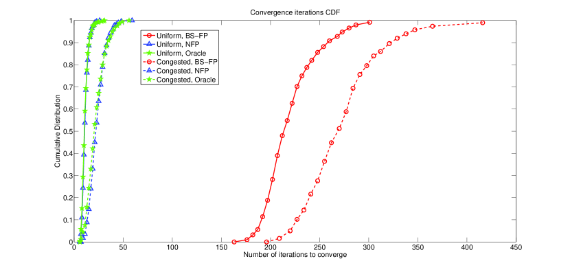
Figure 1: Distribution of the number of iterations required to converge for SISO cellular networks. $N=100$ BSs, $K=160$ users, $\text{SNR}=15$dB.

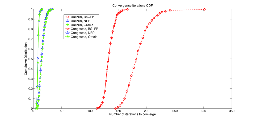
Figure 2: Distribution of the number of iterations required to converge for SIMO cellular networks. $N=100$ BSs, $K=160$ users, $\text{SNR}=10$dB.

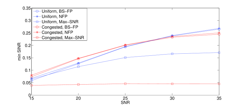
Figure 3: Comparison of the minimum SINR achieved for SISO cellular networks. $N=100$ BSs, $K=160$ users.

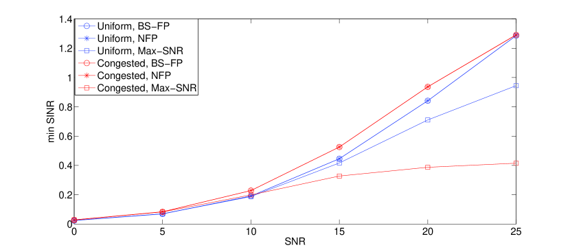
Figure 4: Comparison of the minimum SINR achieved for SIMO cellular networks. $N=100$ BSs, $K=160$ users.

VI Conclusions

In this paper, we investigate the joint BS association and beamforming problem for max-min fairness criterion in the context of UL SIMO cellular networks. We prove the polynomial time solvability of the problem for both SISO and SIMO scenarios by transferring the original problem into a binary search method in conjunction with a series of QoS subproblems which can solved by LP for SISO or SDP for SIMO scenarios, yielding the so-called BS-LP and BS-SDP algorithms. Furthermore, in order to avoid the computational complexity imposed by LP or SDP, we present a BS-FP algorithm where QoS subproblems are solved by a fixed point method. Moreover, for the further reduction of computational complexity, we proposed a novel NFP algorithm which can directly solve the original problem without resorting to the binary search. We show that the NFP algorithm converges to the global optima at a geometric rate. Though we are not able to prove that the NFP algorithm is a polynomial time algorithm, empirically it converges much faster than BS-FP and the provably polynomial time algorithm (BS-LP and BS-SDP). It is a theoretically interesting open question whether the NFP algorithm is a polynomial time algorithm.

Appendix A Proof of Proposition 1

Proof:

We first prove the following fact: if problem (P_SISO-QoS) is feasible, then its optimal power vector $\boldsymbol{p}^{*}$ satisfies the fixed point equation (20). It can be seen that $\frac{p_{k}^{*}}{T_{k}(\boldsymbol{p}^{*})}=\gamma$; otherwise, we can reduce the power $p_{k}^{*}$ to improve the objective function without violating all constraints. As $\boldsymbol{p}^{*}$ satisfies the constraints of (P_SISO-QoS), we have $\bar{\boldsymbol{p}}_{k}\geq p_{k}^{*}=\gamma T_{k}(\boldsymbol{p}^{*})$. Consequently, $p_{k}^{*}=\min\{\gamma T_{k}(\boldsymbol{p}^{*}),\bar{p}_{k}\},\ \forall\ k$, which means that $\boldsymbol{p}^{*}$ satisfies the fixed point equation of (20).

If $\gamma_{\textrm{ach}}=\gamma$, according to (21), we have $\textrm{SINR}_{k}=\frac{q_{k}}{T_{k}(\boldsymbol{q})}\geq\gamma,\forall k$. Based on (20), we have $0\leq q_{k}\leq\bar{p}_{k},\forall k$. Hence $\boldsymbol{q}$ satisfies the constraints of problem (P_SISO-QoS), i.e. $\boldsymbol{q}$ is a feasible solution to (P_SISO-QoS). Assume $\boldsymbol{p}^{*}$ is an optimal power vector to (P_SISO-QoS), then by the argument in the last paragraph $\boldsymbol{p}^{*}$ satisfies (20). As both $\boldsymbol{q}$ and $\boldsymbol{p}^{*}$ are fixed points of (20) and as mentioned earlier that according to [5, Section V.B,Corollary 1] $\boldsymbol{q}$ is the unique fixed point of (20), we have $\boldsymbol{q}=\boldsymbol{p}^{*}$ and $(\bm{q},\bm{b})$ is an optimal solution to (P_SISO-QoS).

If $\gamma_{\textrm{ach}}<\gamma$, according to (21) there exists at least one $q_{k}$ satisfying $q_{k}<\gamma T_{k}(\boldsymbol{q})$ and for this $q_{k}$, based on (20), we have $\bar{p}_{k}=q_{k}<\gamma T_{k}(\boldsymbol{q})$. Assume (P_SISO-QoS) is feasible and its optimal power vector is $\boldsymbol{p}^{*}$, we have $\boldsymbol{p}^{*}=\gamma T_{k}(p^{*})\leq\bar{p}_{k},\ \forall\ k$, thus $\boldsymbol{q}\not=\boldsymbol{p}^{*}$. Therefore, $\boldsymbol{q}$ and $\boldsymbol{p}^{*}$ are two distinct fixed points of (20), which contradicts the the fact that (20) has a unique fixed point. Hence, (P_SISO-QoS) is infeasible. ∎

Appendix B Proof of Lemma 3

Proof:

We can prove this Lemma by following the argument in [20].

Denote

$$f_{n,k}(\boldsymbol{p})=p_{k}\boldsymbol{h}_{n,k}^{H}\boldsymbol{M}_{n}^{-1}(\boldsymbol{p})\boldsymbol{h}_{n,k},\ k=1,\dots,K,\ n=1,\dots,N,$$ (64)

which is a strictly increasing function on $p_{k}\geq 0$ and a decreasing function on $p_{j},j\not=k$ [20, Lemma 3.1].

Suppose there are two distinct solutions $\tilde{\boldsymbol{p}}$ and $\hat{\boldsymbol{p}}$ satisfying Eq.(42), i.e.

$$\max_{n}f_{n,k}(\tilde{\boldsymbol{p}})=\max_{n}f_{n,k}(\hat{\boldsymbol{p}})=\frac{\gamma}{1+\gamma},\;k=1,\dots,K.$$ (65)

Define a nonempty set $\mathcal{K}=\{k\in K\mid\tilde{p}_{k}/\hat{p}_{k}>1\}$ and $k_{0}=\arg\max_{k\in\mathcal{K}}\{\tilde{p}_{k}/\hat{p}_{k}\}$. Define the vector $\boldsymbol{\alpha}=[\alpha_{1},\cdots,\alpha_{K}]$, where $\alpha_{k}$ is given by

$$\alpha_{k}=\left\{\begin{array}[]{ll}\frac{\tilde{p}_{k_{0}}}{\hat{p}_{k_{0}}}>1,&\mbox{if $k\in\mathcal{K}$};\\ 1,&\mbox{otherwise},\end{array}\right.$$ (68)

Consequently, we have

$$f_{n,k_{0}}(\tilde{\boldsymbol{p}}) =f_{n,k_{0}}(\tilde{p}_{k_{0}},\tilde{\boldsymbol{p}}_{-k_{0}})\overset{\textrm{(i)}}{\geq}f_{n,k_{0}}(\tilde{p}_{k_{0}},\boldsymbol{\alpha}_{-k_{0}}\circ\hat{\boldsymbol{p}}_{-k_{0}})$$

$$\overset{\textrm{(ii)}}{=}\alpha_{k_{0}}\hat{p}_{k_{0}}\boldsymbol{h}_{n,k_{0}}^{H}(\sigma_{n}^{2}\boldsymbol{I}+\alpha_{k_{0}}\sum_{j\in\mathcal{K}}\boldsymbol{h}_{n,j}\boldsymbol{h}_{n,j}^{H}\hat{p}_{j}+$$

$$\sum_{j\not\in\mathcal{K}}\boldsymbol{h}_{n,j}\boldsymbol{h}_{n,j}^{H}\hat{p}_{j})^{-1}\boldsymbol{h}_{n,k_{0}}$$

$$\overset{\textrm{(iii)}}{>}\hat{p}_{k_{0}}\boldsymbol{h}_{n,k_{0}}^{H}(\sigma_{n}^{2}\boldsymbol{I}+\sum_{j\in\mathcal{K}}\boldsymbol{h}_{n,j}\boldsymbol{h}_{n,j}^{H}\hat{p}_{j}++$$

$$\sum_{j\not\in\mathcal{K}}\boldsymbol{h}_{n,j}\boldsymbol{h}_{n,j}^{H}\hat{p}_{j})^{-1}\boldsymbol{h}_{n,k_{0}}$$

$$=f_{n,k_{0}}(\hat{\boldsymbol{p}}),$$ (69)

where the notation $\circ$ denotes the Hadamard product, $\tilde{\boldsymbol{p}}_{-k_{0}}$ is the power vector with $k_{0}$th element deleted and $\hat{\boldsymbol{p}}_{-k_{0}}$ as well as $\boldsymbol{\alpha}_{-k_{0}}$ are defined analogously. Moreover, (i) is due to $\tilde{\boldsymbol{p}}_{-k_{0}}\leq\boldsymbol{\alpha}_{-k_{0}}\circ\hat{\boldsymbol{p}}_{-k_{0}}$, (ii) is due to Eq.(68), while (iii) is due to $\alpha_{k_{0}}\hat{p}_{j}>\hat{p}_{j},j\in\mathcal{K}$.

Consequently, we have

$$\max_{n}f_{n,k_{0}}(\tilde{\boldsymbol{p}})>\max_{n}f_{n,k_{0}}(\hat{\boldsymbol{p}})=\frac{\gamma}{1+\gamma},$$ (70)

which contradicts the eq.(65), hence eq.(42) has a unique fixed point. ∎

Appendix C Proof of Lemma 4

Proof:

For a given $\gamma$, if (P_SIMO-QoS-1) is infeasible, suppose $\tilde{\boldsymbol{p}}$ is one optimal solution to (P_SIMO-QoS-2), then $\max_{n\in\{1,\dots,N\}}\tilde{p}_{k}\boldsymbol{h}_{n,k}^{H}\boldsymbol{M}_{n}^{-1}(\tilde{\boldsymbol{p}})\boldsymbol{h}_{n,k}\leq\frac{\gamma}{1+\gamma},\forall k$. We must have $\max_{n\in\{1,\dots,N\}}\tilde{p}_{k}\boldsymbol{h}_{n,k}^{H}\boldsymbol{M}_{n}^{-1}(\tilde{\boldsymbol{p}})\boldsymbol{h}_{n,k}\leq\frac{\gamma}{1+\gamma}$ for some $k$; otherwise $\max_{n\in\{1,\dots,N\}}\tilde{p}_{k}\boldsymbol{h}_{n,k}^{H}\boldsymbol{M}_{n}^{-1}(\tilde{\boldsymbol{p}})\boldsymbol{h}_{n,k}=\frac{\gamma}{1+\gamma},\forall k$, implying that $\tilde{\bm{p}}$ is a feasible solution to (P_SIMO-QoS-1), a contradiction.

If (P_SIMO-QoS-1) is feasible, denote its optimal solution as $\hat{\boldsymbol{p}}$. According to Proposition 3, $\hat{\boldsymbol{p}}$ is the unique solution to (43). Assume $\tilde{\boldsymbol{p}}$ is one solution to (P_SIMO-QoS-2) with $\tilde{\boldsymbol{p}}\not=\hat{\boldsymbol{p}}$. In this case, we have

$$\max_{n}f_{n,k}(\tilde{\boldsymbol{p}})\leq\frac{\gamma}{1+\gamma},\ k=1,\dots,K.$$ (71)

and $\sum_{k=1}^{K}\tilde{p}_{k}\geq\sum_{k=1}^{K}\hat{p}_{k}$.

Define a nonempty set $\mathcal{K}=\{k\in K\mid\tilde{p}_{k}/\hat{p}_{k}>1\}$ and $k_{0}=\arg\max_{k\in\mathcal{K}}\{\tilde{p}_{k}/\hat{p}_{k}\}$. Define the vector $\boldsymbol{\alpha}=[\alpha_{1},\cdots,\alpha_{K}]$, where $\alpha_{k}$ is given by

$$\alpha_{k}=\left\{\begin{array}[]{ll}\frac{\tilde{p}_{k_{0}}}{\hat{p}_{k_{0}}}>1,&\mbox{if $k\in\mathcal{K}$};\\ 1,&\mbox{otherwise},\end{array}\right.$$ (74)

Consequently, we have

$$f_{n,k_{0}}(\tilde{\boldsymbol{p}}) =f_{n,k_{0}}(\tilde{p}_{k_{0}},\tilde{\boldsymbol{p}}_{-k_{0}})\geq f_{n,k_{0}}(\tilde{p}_{k_{0}},\boldsymbol{\alpha}_{-k_{0}}\circ\hat{\boldsymbol{p}}_{-k_{0}})$$

$$=\alpha_{k_{0}}\hat{p}_{k_{0}}\boldsymbol{h}_{n,k_{0}}^{H}(\sigma_{n}^{2}\boldsymbol{I}+\alpha_{k_{0}}\sum_{j\in\mathcal{K}}\boldsymbol{h}_{n,j}\boldsymbol{h}_{n,j}^{H}\hat{p}_{j}++$$

$$\sum_{j\not\in\mathcal{K}}\boldsymbol{h}_{n,j}\boldsymbol{h}_{n,j}^{H}\hat{p}_{j})^{-1}\boldsymbol{h}_{n,k_{0}}$$

$$>\hat{p}_{k_{0}}\boldsymbol{h}_{n,k_{0}}^{H}(\sigma_{n}^{2}\boldsymbol{I}+\sum_{j\in\mathcal{K}}\boldsymbol{h}_{n,j}\boldsymbol{h}_{n,j}^{H}\hat{p}_{j}++$$

$$\sum_{j\not\in\mathcal{K}}\boldsymbol{h}_{n,j}\boldsymbol{h}_{n,j}^{H}\hat{p}_{j})^{-1}\boldsymbol{h}_{n,k_{0}}$$

$$=f_{n,k_{0}}(\hat{\boldsymbol{p}})$$ (75)

Consequently, we have

$$\max_{n}f_{n,k_{0}}(\tilde{\boldsymbol{p}})>\max_{n}f_{n,k_{0}}(\hat{\boldsymbol{p}})=\frac{\gamma}{1+\gamma},$$ (76)

which contradicts Eq.(71).

Consequently, if problems (P_SIMO-QoS-1) is feasible, the problems (P_SIMO-QoS-1) and (P_SIMO-QoS-2) have the same solution. ∎

Appendix D Proof of Lemma 5

Proof:

In order to show that $\tilde{T}_{k}^{n}(\boldsymbol{p})$ is a standard interference function, we need to show three properties:

1. Positivity: For $\boldsymbol{p}\geq\boldsymbol{0}$, $\tilde{T}_{k}^{n}(\boldsymbol{p})>0$;

2. Monotonicity: If $\boldsymbol{p}\geq\boldsymbol{p}^{{}^{\prime}}$, then $\tilde{T}_{k}^{n}(\boldsymbol{p})\geq\tilde{T}_{k}^{n}(\boldsymbol{p}^{{}^{\prime}})$;

3. Scalability: For any $\alpha>1$, $\alpha\tilde{T}_{k}^{n}(\boldsymbol{p})>\tilde{T}_{k}^{n}(\alpha\boldsymbol{p})$.

1) is obvious; 2) can be obtained from [7, Lemma 2 (c)]. In order to show the scalability, we have

$$\tilde{T}_{k}^{n}(\alpha\boldsymbol{p}) =\min_{\|\boldsymbol{u}_{n,k}\|=1}\left\{\frac{\sigma_{a_{k}}^{2}+\alpha\boldsymbol{u}_{n,k}^{H}\sum_{j=1,j\not=k}^{K}p_{j}\boldsymbol{h}_{n,j}\boldsymbol{h}_{n,j}^{H}\boldsymbol{u}_{n,k}}{\boldsymbol{u}_{n,k}^{H}\boldsymbol{h}_{n,k}\boldsymbol{h}_{n,k}^{H}\boldsymbol{u}_{n,k}}\right\}$$

$$<\alpha\min_{\|\boldsymbol{u}_{n,k}\|=1}\left\{\frac{\sigma_{n}^{2}+\boldsymbol{u}_{n,k}^{H}\sum_{j=1,j\not=k}^{K}p_{j}\boldsymbol{h}_{n,j}\boldsymbol{h}_{n,j}^{H}\boldsymbol{u}_{n,k}}{\boldsymbol{u}_{n,k}^{H}\boldsymbol{h}_{n,k}\boldsymbol{h}_{n,k}^{H}\boldsymbol{u}_{n,k}}\right\}$$

$$=\alpha\tilde{T}_{k}^{n}(\boldsymbol{p}).$$ (77)

Hence $\tilde{T}_{k}^{n}(\boldsymbol{p})$ is a standard interference function. ∎

Appendix E Proof of Theorem 4

Proof:

According to Lemma 6, $\boldsymbol{p}^{*}$ is a fixed point of (53). According to the concave Perron-Frobenius theory[17, Theorem 1], we know that (53) has a unique fixed point and the NFP algorithm in Table III converges to this fixed point. Hence, the NFP algorithm in Table III converges to $\boldsymbol{p}^{*}$.

Define $U$ as the set of power vectors $\boldsymbol{p}$ with $\|\boldsymbol{p}\|_{\infty}^{\bar{\boldsymbol{p}}}=1$. It can be verified that

$$A_{k}\leq\tilde{T}_{k}(\boldsymbol{p})\leq B_{k},\ \forall\ \boldsymbol{p}\in U,$$ (78)

where $A_{k}=\min_{n}\min_{\{\|\boldsymbol{u}_{n,k}\|=1\}}\frac{\sigma_{n}^{2}}{\boldsymbol{u}_{n,k}^{H}\boldsymbol{h}_{n,k}\boldsymbol{h}_{n,k}^{H}\boldsymbol{u}_{n,k}}=\min_{n}\frac{\sigma_{n}^{2}}{\|\boldsymbol{h}_{n,k}\|^{2}}$ (note that the second equality is based on the Cauchy-Schwarz inequality of $\|\boldsymbol{u}_{n,k}^{H}\boldsymbol{h}_{n,j}\|^{2}\leq\|\boldsymbol{h}_{n,j}\|^{2}$), and $B_{k}=\tilde{T}_{k}(\bar{\boldsymbol{p}})=\\ \min_{n}\min_{\{\|\boldsymbol{u}_{n,k}\|=1\}}\frac{\sigma_{n}^{2}+\boldsymbol{u}_{n,k}^{H}\sum_{j=1,j\not=k}^{K}\boldsymbol{h}_{n,j}\boldsymbol{h}_{n,j}^{H}\boldsymbol{u}_{n,k}\bar{p}_{j}}{\boldsymbol{u}_{n,k}^{H}\boldsymbol{h}_{n,k}\boldsymbol{h}_{n,k}^{H}\boldsymbol{u}_{n,k}}=\min_{n}\frac{1}{\bar{p}_{k}\boldsymbol{h}_{n,k}\boldsymbol{M}_{n}^{-1}(\bar{\boldsymbol{p}})\boldsymbol{h}_{n,k}}-1$, both of which are constants that only depend on the problem data. Based on (78), we have

$$(1-\kappa)\boldsymbol{e}\leq\tilde{T}(\boldsymbol{p})\leq\boldsymbol{e},\ \forall\ \boldsymbol{p}\in U,$$ (79)

where $\kappa=1-\min_{k}\frac{A_{k}}{B_{k}}\in(0,1)$ and $\boldsymbol{e}=(B_{1},B_{2},\dots,B_{K})>0$. According to the concave Perron-Frobenius Theory [18, Lemma 3, Theorem], the NFP algorithm in Table III converges geometrically at the rate $\kappa$. ∎

References

- [1] R. Sun and Z. Q. Luo, “Globally optimal joint uplink base station association and power control for max-min fairness,” in International Conference on Acoustics, Speech and Signal Processing (ICASSP), 2014.
- [2] A. Khandekar, N. Bhushan, T. Ji, and V. Vanghi, “LTE-advanced: Heterogeneous networks,” in European Wireless Conference (EW), 2010.
- [3] R. Yates and C.-Y. Huang, “Integrated power control and base station assignment,” IEEE Trans. on Vehicular Technology, vol. 44, no. 3, pp. 638–644, 1995.
- [4] S. V. Hanly, “An algorithm for combined cell-site selection and power control to maximize cellular spread spectrum capacity,” IEEE Journal on Selected Areas in Communications, vol. 13, no. 7, pp. 1332–1340, 1995.
- [5] R. Yates, “A framework for uplink power control in cellular radio systems,” IEEE Journal on Selected Areas in Communications, vol. 13, no. 7, pp. 1341–1347, 1995.
- [6] F. Rashid-Farrokhi, K. Liu, and L. Tassiulas, “Downlink power control and base station assignment,” IEEE Communications Letters, vol. 1, no. 4, pp. 102–104, 1997.
- [7] F. Rashid-Farrokhi, L. Tassiulas, and K. J. R. Liu, “Joint optimal power control and beamforming in wireless networks using antenna arrays,” IEEE Transactions on Communications, vol. 46, no. 10, pp. 1437–1450, 1998.
- [8] R. Madan, J. Borran, A. Sampath, N. Bhushan, A. Khandekar, and T. Ji, “Cell association and interference coordination in heterogeneous LTE-A cellular networks,” IEEE Journal on Selected Areas in Communications, vol. 28, no. 9, pp. 1479–1489, 2010.
- [9] M. Hong, R. Sun, H. Baligh, and Z.-Q. Luo, “Joint base station clustering and beamformer design for partial coordinated transmission in heterogeneous networks,” IEEE Journal on Selected Areas in Communications, vol. 31, no. 2, pp. 226–240, 2013.
- [10] R. Sun, H. Baligh, and Z.-Q. Luo, “Long-term transmit point association for coordinated multipoint transmission by stochastic optimization,” in International Workshop on Signal Processing Advances in Wireless Communications (SPAWC), pp. 330–334, 2013.
- [11] Q. Ye, B. Rong, Y. Chen, M. Al-Shalash, C. Caramanis, and J. Andrews, “User association for load balancing in heterogeneous cellular networks,” IEEE Trans. on Wireless Communications, 2012.
- [12] K. Shen and W. Yu, “Downlink cell association optimization for heteregeneous networks via dual coordinate descent,” in International Conference on Acoustics, Speech and Signal Processing (ICASSP), 2013.
- [13] M. Hong and Z.-Q. Luo, “Joint linear precoder optimization and base station selection for an uplink MIMO network: A game theoretic approach,” in International Conference on Acoustics, Speech and Signal Processing (ICASSP), pp. 2941–2944, 2012.
- [14] M. Sanjabi, M. Razaviyayn, and Z.-Q. Luo, “Optimal joint base station assignment and downlink beamforming for heterogeneous networks,” in International Conference on Acoustics, Speech and Signal Processing (ICASSP), pp. 2821–2824, 2012.
- [15] R. Sun, M. Hong, and Z.-Q. Luo, “Optimal joint base station assignment and power allocation in a cellular network,” in International Workshop on Signal Processing Advances in Wireless Communications (SPAWC), pp. 234–238, 2012.
- [16] R. Sun, M. Hong, and Z.-Q. Luo, “Joint downlink base station association and power control for max-min fairness: Computation and complexity,” arXiv preprint arXiv:1407.2791, 2014.
- [17] U. Krause, “Concave Perron–Frobenius theory and applications,” Nonlinear Analysis: Theory, Methods & Applications, vol. 47, no. 3, pp. 1457–1466, 2001.
- [18] U. Krause, “Relative stability for ascending and positively homogeneous operators on Banach spaces,” Journal of Mathematical Analysis and Applications, vol. 188, no. 1, pp. 182–202, 1994.
- [19] Z.-Q. Luo and S. Zhang, “Dynamic spectrum management: Complexity and duality,” IEEE Journal of Selected Topics in Signal Processing, vol. 2, no. 1, pp. 57–73, 2008.
- [20] Y. F. Liu, M. Hong, and Y. H. Dai, “Max-min fairness linear transceiver design problem for a multi-user SIMO interference channel is polynomial time solvable,” IEEE Signal Processing Letters, vol. 20, no. 1, pp. 27–30, 2013.
- [21] M. Bengtsson and B. Ottersten, “Optimal and suboptimal transmit beamforming,” in Handbook of Antennas in Wireless Communications, CRC Press, 2001.
- [22] A. Wiesel, Y. C. Eldar, and S. Shamai, “Linear precoding via conic optimization for fixed mimo receivers,” IEEE Transactions on Signal Processing, vol. 54, no. 1, pp. 161–176, 2006.
- [23] Y.-F. Liu, Y.-H. Dai, and Z.-Q. Luo, “Max-min fairness linear transceiver design for a multi-user MIMO interference channel,” IEEE Transactions on Signal Processing, vol. 61, no. 9, pp. 2413–2423, 2013.
- [24] M. Schubert and H. Boche, “Solution of the multiuser downlink beamforming problem with individual SINR constraints,” IEEE Transactions on Vehicular Technology, vol. 53, no. 1, pp. 18–28, 2004.
- [25] C. Tan, M. Chiang, and R. Srikant, “Fast algorithms and performance bounds for sum rate maximization in wireless networks,” in INFOCOM, pp. 1350–1358, 2009.