The non-equilibrium allele frequency spectrum
in a Poisson random field framework

Abstract

In population genetic studies, the allele frequency spectrum (AFS) efficiently summarizes genome-wide polymorphism data and shapes a variety of allele frequency-based summary statistics. While existing theory typically features equilibrium conditions, emerging methodology requires an analytical understanding of the build-up of the allele frequencies over time. In this work, we use the framework of Poisson random fields to derive new representations of the non-equilibrium AFS for the case of a Wright-Fisher population model with selection. In our approach, the AFS is a scaling-limit of the expectation of a Poisson stochastic integral and the representation of the non-equilibrium AFS arises in terms of a fixation time probability distribution. The known duality between the Wright-Fisher diffusion process and a birth and death process generalizing Kingman’s coalescent yields an additional representation. The results carry over to the setting of a random sample drawn from the population and provide the non-equilibrium behavior of sample statistics. Our findings are consistent with and extend a previous approach where the non-equilibrium AFS solves a partial differential forward equation with a non-traditional boundary condition. Moreover, we provide a bridge to previous coalescent-based work, and hence tie several frameworks together. Since frequency-based summary statistics are widely used in population genetics, for example, to identify candidate loci of adaptive evolution, to infer the demographic history of a population, or to improve our understanding of the underlying mechanics of speciation events, the presented results are potentially useful for a broad range of topics.

1 Introduction

The allele frequency spectrum (AFS) describes the distribution of allele frequencies over a large number of identical and independent loci. In practice, the AFS is approximated by allele frequencies recorded in a sample of individuals. Here, the recent progress in whole-genome re-sequencing has significantly improved the accessibility of the AFS, and several allele frequency-based summary statistics have become central measurements in population genetic studies. The estimation of the AFS is then often based on polymorphic nucleotide sites, where the frequency of the derived allele over a finite collection of sites in the sample is summarized. In this context, the otherwise equivalent term ‘site frequency spectrum’ (SFS) is frequently used. For the purpose of generality, we here use the term AFS.

The theory on the AFS was initiated in the 1930s with the classical work of Fisher and Wright in a framework of diffusion theory including effects of natural selection [Fisher, 1930, Wright, 1931, 1938]. Subsequently, Kimura [1964] pioneered the systematic use of stochastic processes in population genetics, and developed the theory further. In particular, he considered the equilibrium distribution of allele frequencies under irreversible mutation in an ensemble of polymorphic loci [Kimura, 1970b]. Central to these successful applications of diffusion theory in describing the equilibrium limit AFS for various mutation and selection scenarios is the Green function representation of diffusion process occupation time functionals [Karlin and Taylor, 1981]. Then, in order to study the impact of natural selection on the number of fixations in diverging species, Sawyer and Hartl [1992] introduced the Poisson random field framework. The basic assumptions of this approach are that new mutant alleles arise at Poisson times, mutations are irreversible, and the frequencies of the descendants of each mutation are described by independent Markov processes (no linkage). The loss or fixation of a mutant allele is captured by the separate events of extinction or fixation of the Markov process. The collection of Markov processes form a Poisson random field in the sense that the limiting distributions of the allele frequencies are independent Poisson random variables. In particular, the number of fixations is a Poisson random variable with expected value increasing linearly over time. Segregating mutations are, on the other hand, in equilibrium with respect to time, and hence the marginal distributions of the corresponding Poisson variables are stationary. In other words, the AFS is assumed to be in equilibrium with respect to time.

More recently, Evans et al. [2007] initiated the study of the non-equilibrium AFS in a single population including effects of natural selection, in the sense of deriving a function $f(t,x)$ which represents the expected fraction of alleles of frequency $x$ existing at some time $t$, given an initial fraction $f(0,x)$ of alleles at time $t=0$. Some of the modeling parameters, such as population size and selection intensity, are also allowed to depend on time. The resulting non-equilibrium AFS $f(t,x)$ is provided as a solution to a partial differential equation (PDE), essentially the Kolmogorov forward equation for the corresponding diffusion, linked to a given rate of mutational influx via a specific boundary condition of $f(t,x)$ as $x\to 0$. An additional approximation method using moments is employed to study the resulting allele frequencies in a sample. Building on this approach, Zivkovic and Stephan [2011] provide analytical results on the non-equilibrium AFS for the neutral case, focusing on time-dependence arising due to changes in population size. In the same direction, Zivkovic et al. [2015] consider the case of natural selection and develop the moment approximation method for a scenario of piecewise-constant population size starting from an equilibrium.

In a parallel methodological track the AFS has been studied using the view of coalescent theory, where mutations are randomly placed on the branches of a genealogy of a sample of individuals [Kingman, 1982]. First, Fu [1995] obtained a representation of the stationary AFS for a single population under the assumptions of neutrality and constant population size, by deriving mean and variance of the number of mutations on each branch of a given length. Griffiths and Tavaré [1998] explored the duality relation between the neutral Wright-Fisher diffusion process and Kingman’s pure death coalescent process further and addressed deterministic changes in population size. Moreover, Wakeley and Hey [1997] obtained a description of the joint AFS of two isolated populations descending from a common ancestor under neutrality. Chen [2012] elaborated on their work and extended it to multiple populations and also modeled scenarios such as selective sweeps, influx of migration and changes in population size.

Here, we build on the work of Sawyer and Hartl [1992] and develop the approach of Mugal et al. [2014] further to derive a representation of the non-equilibrium AFS as the limiting expected value of a suitable Poisson stochastic integral. The model is developed in steps starting with finite population size $N$ and sequences of $L$ sites, subject to mutational influx of derived alleles and Wright-Fisher reproduction in discrete generation time. Assuming mutation and selection rates per individual and generation of order $1/N$ and evolutionary time $t$ counting $Nt$ generations, we then apply the continuous time Wright-Fisher diffusion approximation, but follow Evans et al. [2007] in keeping $N$ as a modeling parameter. In a next stage of approximation the mutation rate per site tends to zero with preserved over-all mutation rate for sequences, a procedure which we interpret and implement as a limit in distribution as $L\to\infty$. The result is a Poisson random field parametrized by $N$, which we study in some detail. Then, we find the limiting expected values as $N\to\infty$ and identify the time-dependent AFS which arises in the limit. Thereby, we provide a link between the Poisson random field approach by Sawyer and Hartl [1992] and the setting of Evans et al. [2007], in particular by identifying the PDE solution $f(t,x)$ in terms of a Wright-Fisher fixation time probability distribution. An additional representation is obtained by elaborating on the duality relation between the Wright-Fisher diffusion process and a class of birth and death processes, where birth rates are proportional to the strength of selection [Shiga and Uchiyama, 1986, Athreya and Swart, 2005].

2 Poisson random field model

2.1 Basic Markov chain model

A population consists of $N$ individuals, where each individual is represented by a sequence of $L$ sites. Random mutation events act on sites, independently and uniformly over individuals, replacing an ancestral allele by a derived. Only mono-allelic sites are affected by mutation. Thus, the setting of the model only allows for two alleles, the derived and the ancestral, in each site. The composition of ancestral and derived alleles per site changes in discrete steps from one generation to the next according to the Wright-Fisher reproduction with selection, which relies on the following assumptions 1) non-overlapping generations, 2) constant population size and 3) random mating. The population dynamics is then given by a collection of independent, identically distributed Markov chains in discrete time, $\{(X^{i}_{n})_{n\geq 0},1\leq i\leq L\}$, one component for each site. The state variable is

$$X^{i}_{n}=\mbox{\# of individuals in generation $n$ with the derived allele in site $i$}$$

and the state space of each chain is $\{0,1,\dots,N\}$. An example path of the Markov chain is visualized in Figure 1. Site $i$ is said to be mono-allelic at time $n$ if it carries the ancestral allele throughout the entire population, so that $X^{i}_{n}=0$. A trajectory $(X^{i}_{n})_{n\geq 0}$ consists of subsequent mono-allelic periods in state $0$ and active polymorphic periods with both ancestral and derived alleles present. Whenever a derived allele reaches fixation in generation $n$, that is $X_{n}^{i}=N$, then the derived is declared to be the new ancestral allele at that site.

We let $\mu>0$ be the mutation probability

$$\mu=$$ probability per individual and generation that an ancestral is replaced

$$\textrm{ by the derived allele at a single mono-allelic site},$$

and for each generation $n$ and site $i$, we let $J^{i}_{n}$ be binomially distributed independent random variables, such that for $i=1,\dots,L$, $n\geq 1$,

$$J_{n}^{i}=\mbox{\# of mutations in generation $n$ hitting a mono-allelic site $i$}\in\mathrm{Bin}(N,\mu).$$

In the limit of small mutation rate $\mu\to 0$, such that $N\mu$ is a small probability, we have

$$P(J_{n}^{i}=0)=(1-\mu)^{N}=1-N\mu+o(N\mu)$$

as well as

$$P(J_{n}^{i}=1)=N\mu+o(N\mu),\quad P(J_{N}^{i}\geq 2)=o(N\mu).$$

Hence, given $X_{n}^{i}$ in generation $n$, the random variable

$$J^{i}_{n+1}1_{\{X^{i}_{n}=0\}}=\mbox{\# of mutations in site $i$ at generation $n+1$}$$

is approximately $\mathrm{Bin}(1,N\mu)$ distributed, for each $i$. It is the injection of new derived alleles in the population at mono-allelic sites, and the change-of-state of the Markov chain from $0$ to $1$, which marks the beginning of the active periods. To make the dynamics during active periods precise, we let $s$, $s\geq-1$, denote the coefficient of selection. Then, conditionally given $X_{n}^{i}=k$ derived alleles at site $i$ in the parental generation $n$, the number of offspring derived alleles for the next generation $n+1$ is a binomially distributed random variable $H^{i}_{n+1}$, such that

$$H_{n+1}^{i}\in\mathrm{Bin}(N,p_{k}),\quad p_{k}=\frac{k(1+s)}{k(1+s)+(N-k)\cdot 1}.$$

Here, the case $k=N$ represents fixation of the derived allele and hence the substitution of a former ancestral type with a derived in site $i$. In our context, however, the derived is redefined to be the new ancestral type from generation $n+1$ and onwards, and therefore the offspring $H^{i}_{n+1}=N$ will not count towards $X_{n+1}^{i}$. Summing up, given an initial distribution of $X_{0}=(X_{0}^{1},\dots,X_{0}^{L})$, the components of the discrete time Markov chain $X_{n}=(X^{1}_{n},\dots,X_{n}^{L})$, are defined recursively by

$$X_{n+1}^{i}=H_{n+1}^{i}-N1_{\{X_{n}^{i}=N\}}+J^{i}_{n+1}1_{\{X^{i}_{n}=0\}},\quad n\geq 0,\quad 1\leq i\leq L.$$

It follows that a mono-allelic site remains mono-allelic for a geometrically distributed number of generations until a single mutation hits after an average number of $1/N\mu$ generations.

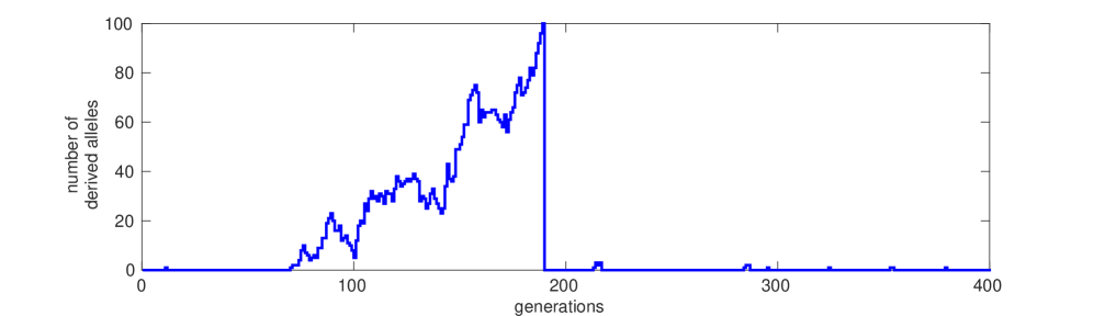
Figure 1: Simulation of a single path $\{X_{n},0\leq n\leq 400\}$ for the case $N=100$, $s=0$, and $\mu=2\cdot 10^{-4}$. A site is referred to as mono-allelic if $X_{n}=0$. Once a mutation hits a site, the site becomes polymorphic $0<X_{n}<N$, i.e. both the ancestral and the derived allele are segregating in the population. The ultimate fate of the derived allele is either extinction, $X_{n}=0$, or fixation, $X_{n}=N$. However, whenever a derived allele reaches fixation in generation $n$, then the derived allele is declared to be the new ancestral allele at that site, in other words $X_{n}$ is set to $0$.

2.2 Diffusion approximation

For the transition to a continuous time Markov chain we introduce the scaled parameters $\theta>0$ and $\gamma$ defined by

$$\theta =LN\mu=\mbox{mutation intensity per sequence and generation}$$

$$\gamma =Ns=\mbox{selection intensity per site and generation}.$$

Along the relevant evolutionary time scale, $t$ units of time correspond to $[Nt]$ generations. On this scale the total mutation rate is $N\theta$ per sequence and time unit. We define the time-scaled allele frequencies $X_{N}(t)=(X_{N}^{1}(t),\dots,X_{N}^{L}(t))$ by

$$X_{N}^{i}(t)=N^{-1}X_{[Nt]}^{i},\quad 1\leq i\leq L,\quad t\geq 0.$$

Then, with $h\sim 1/N$ denoting a small evolutionary time step,

$$X^{i}_{N}(t+h)-X^{i}_{N}(t)=\frac{1}{N}H^{i}_{[Nt]+1}-1_{\{X^{i}_{N}(t)=1\}}-X^{i}_{N}(t)+\frac{1}{N}J^{i}_{[Nt]+1}1_{\{X^{i}_{N}(t)=0\}}.$$

Furthermore, by evaluating conditional expectations for each term, for $x\in\{0,1/N,\dots,1\}$,

$$\mathbb{E}[X^{i}_{N}(t+h)-X^{i}_{N}(t)|X^{i}_{N}(t)=x] =h\Big{(}\frac{\gamma x(1-x)}{1+x\gamma/N}\,1_{\{1/N\leq x<1\}}+\mu N\,1_{\{x=0\}}\Big{)}$$

$$\approx h\Big{(}\gamma x(1-x)\,+\frac{\theta}{L}\,1_{\{x=0\}}\Big{)},$$

where the approximation in the last step comes from ignoring the term multiplied by $\gamma/N$. Similarly, by computing second moments,

$$\mathbb{E}[(X^{i}_{N}(t+h)-X^{i}_{N}(t))^{2}|X^{i}_{N}(t)=x] =h\Big{(}x(1-x)+\frac{\theta}{NL}\,1_{\{x=0\}}\Big{)}$$

$$\approx h\,x(1-x).$$

The above relations of first and second moments are the approximative drift and variance functions for the Wright-Fisher diffusion process with selection, and with the additional mechanism of returns from state $0$ to state $1/N$ with intensity $N\theta/L$ per site. The Wright-Fisher diffusion process arises in the limit of weak convergence of the Wright-Fisher reproduction model as the population size $N$ tends to infinity. Letting $(W_{t})_{t\geq 0}$ be a standard Brownian motion, the Wright-Fisher diffusion process with scaled selection coefficient $\gamma$, is the Markov process $(\xi_{t})_{t\geq 0}$ with state space $[0,1]$ defined as the unique strong solution of the stochastic differential equation

$$d\xi_{t}=\beta(\xi_{t})\,dt+\sigma(\xi_{t})\,dW_{t},\quad t\geq 0,\quad\xi_{0}=x\in(0,1),$$

with drift function $\beta(x)$ and variance function $\sigma^{2}(x)$ given by

$$\beta(x)=\gamma x(1-x),\quad\sigma^{2}(x)=x(1-x).$$

The case $\gamma=0$ is the neutral Wright-Fisher diffusion process, $\gamma>0$ corresponds to positive selection and $\gamma<0$ to negative selection. Formally, we assume that the paths $(\xi_{t})$ are elements in the class $\mathcal{D}$ of functions defined on the real line $\mathbb{R}$ with values in the unit interval $[0,1]$, which are continuous from the right and have limits from the left. We write $\mathbb{P}^{\gamma}_{x}$ for the probability measure and $\mathbb{E}^{\gamma}_{x}$ for the expectation of the process in $\mathcal{D}$, given that $\xi_{0}=x$. It is convenient in the current setting to consider in addition time-shifted processes, initiated at an arbitrary time $s$. For such an $s$, let $\mathbb{P}_{x}^{\gamma}(d\xi^{s})$ be the law of the Wright-Fisher diffusion process with selection coefficient $\gamma$ and paths $(\xi^{s}_{u})$ in $\mathcal{D}$ with initial time $s$ and initial value $x$, that is $\xi_{u}^{s}=0$, $u<s$, and $\xi_{s}^{s}=x$. This is the strong solution of the stochastic differential equation

$$d\xi^{s}_{t}=\gamma\xi^{s}_{t}(1-\xi^{s}_{t})\,dt+\sqrt{\xi^{s}_{t}(1-\xi^{s}_{t})}\,dW_{t},\quad t\geq s,\quad\xi^{s}_{s}=x.$$

We use the same notations $\mathbb{P}_{x}^{\gamma}$ and $\mathbb{E}_{x}^{\gamma}$ for the probability measure and expectation without explicit mentioning of the initial time $s$, which will be clear from context. With initial value $x$, $0<x<1$, the process either gets fixed in $x=1$ or goes extinct in $x=0$ with the corresponding fixation time $\tau_{1}$, extinction time $\tau_{0}$, and absorption time $\tau=\tau_{0}\wedge\tau_{1}$ the minimum of $\tau_{0}$ and $\tau_{1}$. In this sense both points $\{0,1\}$ are classified as boundary exit points. The exit measure is given by the fixation probability

$$q_{\gamma}(x)=\mathbb{P}_{x}^{\gamma}(\tau_{1}<\infty)=\frac{1-e^{-2\gamma x}}{1-e^{-2\gamma}},\quad\gamma\not=0,\qquad q_{0}(x)=\mathbb{P}_{x}^{0}(\tau_{1}<\infty)=x.$$ (1)

Based on these observations we now introduce a continuous time Markov process $Y_{N,L}(t)=(Y_{N,L}^{1}(t),\dots,Y_{N,L}^{L}(t))$, which is our final population model for the case of large but finite $N$ and fixed $L$. An example of such a process is visualized in Figure 2. The components $Y_{N,L}^{i}(t)$ of $Y_{N,L}$ have state space given by the continuous interval $[0,1)$ and jumps from the boundary. The paths are cyclic with each cycle consisting of one mono-allelic period in state $0$ and one polymorphic period of non-zero frequency. The mono-allelic periods are exponentially distributed with intensity $N\theta/L$. During an active period, starting at time $s$, the path is a Wright-Fisher diffusion process $(\xi^{s}_{t})_{t\geq s}$ with initial state $1/N$. The duration of the active period is the absorption time $\tau$. The result is either fixation, which occurs with the scaled fixation probability

$$\mathbb{P}_{1/N}^{\gamma}(\tau_{1}<\infty)\approx\frac{\omega_{\gamma}}{N},\quad\omega_{\gamma}=\lim_{N\to\infty}Nq_{\gamma}(1/N)=\frac{2\gamma}{1-e^{-2\gamma}},\quad\omega_{0}=1,$$ (2)

or, otherwise, extinction. The end of the active period marks the beginning of a new mono-allelic period, hence a new cycle. The previously studied frequency processes $X^{i}_{N}(t)$, are discrete state approximations of $Y_{N,L}^{i}(t)$. The collection of allele frequencies $Y_{N,L}^{i}(t)>0$ over all $L$ sites constitutes the AFS at time $t$. Three example AFS are depicted by the histograms shown in the lower panel of Figure 2.

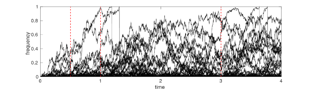
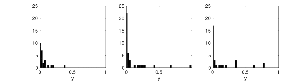
Figure 2: Upper panel: a simulation of $Y_{N,L}(t)$, $0\leq t\leq 4$, for a population of size $N=500$ consisting of $L=1500$ sites, which are all mono-allelic at $t=0$ and evolve neutrally, $\gamma=0$, with a mutation rate $\theta=3$. Each black line represents the path of the derived allele frequency at one of the $L=1500$ sites. The three vertical red dashed lines mark the time points $t=0.5,1,3$, for which the AFS is depicted by histograms. Lower panel: the three histograms display the AFS for the time points $t=0.5,1,3$ from left to right, which illustrates the build-up of higher allele frequencies with time.

2.3 Poisson random field approximation

The next stage in developing the model is concerned with calibrating the length of the sequences measured in sites, $L$, with the strength of mutation per site, $N\theta/L$. The basic observation is that the number of new mutations per time unit in $L$ mono-allelic sites is $\mathrm{Bin}(L,N\theta/L)$, hence for large $L$ but fixed population size $N$, approximately Poisson with mean $N\theta$. Rather than visualizing infinitely long sequences it is convenient therefore to imagine a spatially continuous sequence (of length one, say), where polymorphic “Poisson sites” are placed according to a Poisson process with intensity $N\theta$.

The collection of allele frequencies over all $L$ sites $\{Y_{N,L}(t),t\geq 0\}$ form a random field $\mathcal{X}_{t}^{N,L}$ on the positive real line, in the sense

$$t\mapsto\mathcal{X}_{t}^{N,L}=\sum_{i=1}^{L}\delta_{Y_{N,L}^{i}(t)},\quad t\geq 0.$$

For bounded functions $f:[0,1]\to\mathbb{R}$ on the unit interval $[0,1]$ we use the bracket notation $\langle\mathcal{X}_{t}^{N,L}\!,f\rangle$ for the application of the random field to $f$, and evaluate the combined effect of all sites by

$$t\mapsto\langle\mathcal{X}_{t}^{N,L}\!,f\rangle=\sum_{i=1}^{L}f(Y_{N,L}^{i}(t)).$$

To handle the limit operations as $L$ and, later, $N$ tend to infinity, we specify the set of functions

$$\mathcal{F}=\{f:[0,1]\to\mathbb{R},\;\mbox{$f$ bounded},\;f(0)=0,\;\int_{0}^{1}y^{-1}|f(y)|\,dy<\infty\},$$

and the further restricted subset

$$\mathcal{F}_{0}=\{f\in\mathcal{F}:f(1)=0\}.$$

The class $\mathcal{F}_{0}$ enters naturally studying properties of the Wright-Fisher diffusion process based on the Green function and occupation time functional for diffusion processes, [Karlin and Taylor, 1981, Breiman, 1992].

The scale function $S_{\gamma}(x)$ and speed function $m_{\gamma}(x)$ associated with the Wright-Fisher diffusion process with selection parameter $\gamma$ are

$$S_{0}(x)=x,\quad S_{\gamma}(x)=\frac{1}{2\gamma}(1-e^{-2\gamma x}),\quad\gamma\not=0,\qquad m_{\gamma}(x)=\frac{e^{2\gamma x}}{x(1-x)}.$$

By integration with respect to the Green function $G_{\gamma}(x,y)$, defined as

$$G_{\gamma}(x,y)=\left\{\begin{array}[]{lc}2q_{\gamma}(x)(S_{\gamma}(1)-S_{\gamma}(y))m(y),&0\leq x\leq y\leq 1\\[5.69054pt] 2(1-q_{\gamma}(x))(S_{\gamma}(y)-S_{\gamma}(0))m(y),&0\leq y\leq x\leq 1,\end{array}\right.$$

one obtains the time occupation functional

$$\mathbb{E}^{\gamma}_{x}\Big{[}\int_{0}^{\tau}g(\xi_{t})\,dt\Big{]}=\int_{0}^{1}G_{\gamma}(x,y)g(y)\,dy.$$ (3)

Using the functions

$$\pi_{\gamma}(y)=\frac{1-e^{-2\gamma(1-y)}}{\gamma y(1-y)},\quad\widetilde{\pi}_{\gamma}(y)=\frac{e^{2\gamma y}-1}{\gamma y(1-y)},\quad\gamma\not=0$$

and

$$\pi_{0}(y)=\frac{2}{y}\quad\widetilde{\pi}_{0}(y)=\frac{2}{1-y}$$

we have

$$G_{\gamma}(x,y)=q_{\gamma}(x)\,1_{\{x<y\}}\pi_{\gamma}(y)+(1-q_{\gamma}(x))\,1_{\{x>y\}}\widetilde{\pi}_{\gamma}(y)$$

and

$$\int_{0}^{1}G_{\gamma}(x,y)g(y)\,dy=q_{\gamma}(x)\int_{x}^{1}g(y)\pi_{\gamma}(y)\,dy+(1-q_{\gamma}(x))\int_{0}^{x}g(y)\widetilde{\pi}_{\gamma}(y)\,dy$$ (4)

whenever the integrals on the right hand side are well-defined. It is now straightforward to derive from (3) and (4), and also using the parameter $\omega_{\gamma}$ introduced in (2), the following well-known and fundamental limit property of Wright-Fisher diffusion processes:

$$\lim_{N\to\infty}N\mathbb{E}_{1/N}^{\gamma}\int_{0}^{\tau}f(\xi_{s})\,ds=\omega_{\gamma}\int_{0}^{1}f(y)\pi_{\gamma}(y)\,dy,\quad f\in\mathcal{F}_{0},$$ (5)

where $\omega_{\gamma}\,\pi_{\gamma}(y)$ is known as the allele frequency spectrum.

We are now in position to introduce a random field $\mathcal{X}_{t}^{N}$, which arises from $\mathcal{X}_{t}^{N,L}$ in the limit $L\to\infty$. We first construct $\mathcal{X}_{t}^{N}$ as a stochastic integral with respect to a Poisson measure, see e.g. [Kallenberg, 2002], and then establish the convergence in $L$. Let $n_{N}(ds,d\xi^{s})$ be the product measure defined on $\mathbb{R}^{+}\times\mathcal{D}$ by

$$n_{N}(ds,d\xi^{s})=N\theta\,ds\,\mathbb{P}_{1/N}^{\gamma}(d\xi^{s})$$

and let $\mathcal{N}_{N}(ds,d\xi^{s})$ be a Poisson random measure on $\mathbb{R}^{+}\times\mathcal{D}$ with intensity measure given by $n_{N}$. For $t\geq 0$, we let $\mathcal{X}_{t}^{N}$ be the Poisson random field defined by the stochastic integral

$$\langle\mathcal{X}_{t}^{N}\!,f\rangle=\int_{\mathbb{R}^{+}\times\mathcal{D}}f(\xi^{s}_{t})\,\mathcal{N}_{N}(ds,d\xi^{s}).$$

Proposition 1.

The stochastic integral $\langle\mathcal{X}^{N}_{t}\!,f\rangle$ is well-defined with finite expected value, such that, for every $f\in\mathcal{F}_{0}$,

$$\mathbb{E}\langle\mathcal{X}^{N}_{t}\!,f\rangle=N\theta\,\mathbb{E}^{\gamma}_{1/N}\Big{[}\int_{0}^{t\wedge\tau}f(\xi^{0}_{u})\,du\Big{]}<\infty$$

and, for $f\in\mathcal{F}$ and fixed $t$,

$$\mathbb{E}\langle\mathcal{X}^{N}_{t}\!,f\rangle=N\theta\,\mathbb{E}^{\gamma}_{1/N}\Big{[}\int_{0}^{t}f(\xi^{0}_{u})\,du\Big{]}<\infty.$$

Proof.

For the existence and finite expectation of the Poisson integral it is sufficient to show

$$\int_{\mathbb{R}^{+}\times\mathcal{D}}|f(\xi^{s}_{t})|\,n_{N}(ds,d\xi^{s})=N\theta\mathbb{E}^{\gamma}_{1/N}\int_{0}^{t\wedge\tau}|f(\xi_{t}^{s})|\,ds<\infty.$$

However, for $f\in\mathcal{F}_{0}$ the right hand side is bounded by

$$N\theta\mathbb{E}^{\gamma}_{1/N}\int_{0}^{\tau}|f(\xi_{t}^{s})|\,ds=N\theta\int_{0}^{1}G_{\gamma}(1/N,y)|f(y)|\,dy,$$

which is finite for every $N$ and, moreover, has a finite limit as $N\to\infty$. Thus, $\langle\mathcal{X}^{N}_{t}\!,f\rangle$ exists with finite expected value

$$N\theta\mathbb{E}^{\gamma}_{1/N}\int_{0}^{t\wedge\tau}f(\xi^{s}_{t})\,ds=N\theta\mathbb{E}^{\gamma}_{1/N}\int_{0}^{t\wedge\tau}f(\xi^{0}_{u})\,du.$$

A similar argument shows the claim for $f\in\mathcal{F}$ and fixed $t$. ∎

Proposition 2.

Let $f\in\mathcal{F}_{0}$. The allele frequency random field $\langle\mathcal{X}_{t}^{N,L}\!,f\rangle$ converges as $L$ tends to infinity to the Poisson random field $\langle\mathcal{X}_{t}^{N}\!,f\rangle$,

$$\{\langle\mathcal{X}_{t}^{N,L}\!,f\rangle,\;t\geq 0\}\Rightarrow\{\langle\mathcal{X}_{t}^{N}\!,f\rangle,\;t\geq 0\},$$

in the sense of convergence of random processes in finite-dimensional distribution.

The proof of this proposition employs an indexing method using measures, which amounts to taking the limit as $L\to\infty$ of the quantities

$$\int\langle\mathcal{X}_{u}^{N,L}\!,f\rangle\,\mu(du),$$

for a suitable class of measures $\mu$. This technique has been used for other random fields elsewhere, and the technical aspects are not central for the specific problem at hand. Therefore, the proof is given separately in Section 6.

2.4 The stationary functional

In our approach, we start from a completely mono-allelic state at time $t=0$, where $\langle\mathcal{X}_{t}^{N}\!,f\rangle$, $t\geq 0$, represents the non-equilibrium build-up of allele frequencies towards a steady-state spectrum of frequencies in the limit $t\to\infty$. One way of identifying such an asymptotic limit is achieved by tuning the initial state of the process to obtain a stationary system. Here, the appropriate initial state is obtained simply by including all mutations which occurred at some time $s<0$ and counting the resulting frequencies $\xi_{t}^{s}$ at time $t>0$. The result is a stationary version $\langle\mathcal{X}_{\infty}^{N},f\rangle$ of the population functional $\langle\mathcal{X}_{t}^{N}\!,f\rangle$. Indeed, observing that $f\in\mathcal{F}_{0}$ implies $g=e^{\alpha f}-1\in\mathcal{F}_{0}$,

$$\langle\mathcal{X}_{t}^{N}\!,f\rangle=\int_{\mathbb{R}_{+}\times\mathcal{D}}f(\xi^{s}_{t})\,\mathcal{N}_{N}(ds,d\xi^{s}),\quad f\in\mathcal{F}_{0},$$

has the Laplace functional

$$\ln\mathbb{E}\exp\{\alpha\langle\mathcal{X}_{t}^{N}\!,f\rangle\} =N\theta\,\mathbb{E}_{1/N}^{\gamma}\Big{[}\int_{0}^{t\wedge\tau}(e^{\alpha f(\xi^{s}_{t})}-1)\,ds\Big{]}$$

$$=N\theta\,\mathbb{E}_{1/N}^{\gamma}\Big{[}\int_{0}^{t\wedge\tau}(e^{\alpha f(\xi^{0}_{u})}-1)\,du\Big{]},$$

which converges as $t\to\infty$ to

$$N\theta\,\mathbb{E}_{1/N}^{\gamma}\Big{[}\int_{0}^{\tau}(e^{\alpha f(\xi^{0}_{u})}-1)\,du\Big{]}=\ln\mathbb{E}\exp\{\alpha\langle\mathcal{X}_{\infty}^{N},f\rangle\}.$$

Here, the intensity measure of

$$\langle\mathcal{X}_{\infty}^{N},f\rangle=\int_{\mathbb{R}\times\mathcal{D}}f(\xi^{s}_{t})\,\mathcal{N}_{N}(ds,d\xi^{s})$$

in the variable $s$ extends to all of the real line. Furthermore, by (5),

$$\lim_{N\to\infty}\ln\mathbb{E}\exp\{\alpha\langle\mathcal{X}_{\infty}^{N},f\rangle\}=\theta\omega_{\gamma}\int_{0}^{1}(e^{\alpha f(y)}-1)\pi_{\gamma}(y)\,dy.$$

Hence $\langle\mathcal{X}_{\infty}^{N},f\rangle$ converges in distribution as $N\to\infty$ to the stochastic integral

$$\langle\mathcal{X}_{\infty},f\rangle=\int f(y)\,\mathcal{N}(dy),$$ (6)

where $\mathcal{N}(dy)$ is a Poisson random measure on $[0,1]$ with intensity measure $\theta\omega_{\gamma}\pi_{\gamma}(y)dy$.

3 The non-equilibrium allele frequency spectrum

The limiting Poisson intensity $\omega_{\gamma}\pi_{\gamma}(y)dy$ of the stationary model $\mathcal{X}_{\infty}$ in (6) appeared in (5) as the kernel of a scaled occupation time functional. The main theoretical result in this work is the derivation of the fixed time and large population size limit of the Poisson integral expectations

$$\lim_{N\to\infty}\mathbb{E}^{\gamma}\langle\mathcal{X}_{t}^{N}\!,f\rangle$$

in Proposition 1. In doing so we obtain a non-equilibrium version of the AFS which represents the build-up of frequencies over a time period $[0,t]$. To simplify notation from now on we write $(\xi_{t})_{t\geq 0}$ (rather than $(\xi^{0}_{t})$) for the the Wright-Fisher diffusion process with initial time $t=0$. Then

$$\mathbb{E}\langle\mathcal{X}_{t}^{N}\!,f\rangle=\theta N\mathbb{E}_{1/N}^{\gamma}\int_{0}^{t}f(\xi_{u})\,du,\quad f\in\mathcal{F}$$

and

$$N\mathbb{E}_{1/N}^{\gamma}\int_{0}^{t}f(\xi_{u})\,du=N\mathbb{E}_{1/N}^{\gamma}\int_{0}^{t\wedge\tau}f(\xi_{u})\,du,\quad f\in\mathcal{F}_{0}.$$

3.1 Representation in terms of the probability distribution of the time to fixation

Let $\mathbb{P}^{*\gamma}_{x}$ and $\mathbb{E}^{*\gamma}_{x}$ be the distribution and expectation of the Wright-Fisher diffusion process with selection coefficient $\gamma$ conditioned on the event of fixation, $\tau_{1}<\infty$. Then, by symmetry,

$$\mathbb{P}^{\gamma}_{x}(\tau<t) =\mathbb{P}^{\gamma}_{x}(\tau_{1}<t)+\mathbb{P}^{\gamma}_{x}(\tau_{0}<t)$$

$$=\mathbb{P}^{*\gamma}_{x}(\tau_{1}<t)q_{\gamma}(x)+\mathbb{P}^{*-\gamma}_{1-x}(\tau_{1}<t)(1-q_{\gamma}(x)),$$

where $q_{\gamma}(x)$ is the fixation probability defined in (1). For the neutral case $\gamma=0$, the fixation time distribution given that fixation occurs is given by [Kimura, 1970a]

$$\mathbb{P}_{x}^{*0}(\tau_{1}>t)=(1-x)\sum_{i=2}^{\infty}(2i-1)(-1)^{i}H([2-i,i+1],[2],x)\,e^{-\binom{i}{2}t},$$ (7)

where $H$ is the hypergeometric function. In particular,

$$\mathbb{P}_{0}^{*0}(\tau_{1}>t)=\sum_{i=2}^{\infty}(2i-1)(-1)^{i}\,e^{-\binom{i}{2}t}.$$

The time-dependent integration kernel of the non-equilibrium AFS turns out to be $\omega_{\gamma}\mathbb{P}^{*\gamma}_{1-y}(\tau_{1}\leq t)\,\pi_{\gamma}(y)dy$, in the sense of the following result.

Theorem 1.

Let $f\in\mathcal{F}_{0}$. Then

$$\lim_{N\to\infty}\mathbb{E}\langle\mathcal{X}_{t}^{N}\!,f\rangle =\theta\omega_{\gamma}\int_{0}^{1}f(y)\,\mathbb{P}^{*\gamma}_{1-y}(\tau_{1}\leq t)\pi_{\gamma}(y)\,dy$$ (8)

$$=\theta\int_{0}^{1}f(y)\frac{\mathbb{P}^{\gamma}_{1-y}(\tau_{1}\leq t)}{1-y}\pi_{0}(y)\,dy$$ (9)

More generally, if $f\in\mathcal{F}$, then

$$\lim_{N\to\infty}\mathbb{E}\langle\mathcal{X}_{t}^{N}\!,f\rangle=\theta\omega_{\gamma}\int_{0}^{1}(f(y)-f(1)q_{\gamma}(y))\,\mathbb{P}_{1-y}^{*\gamma}(\tau_{1}\leq t)\pi_{\gamma}(y)\,dy+\theta f(1)\omega_{\gamma}\,t$$

and

$$\lim_{N\to\infty}N\mathbb{E}_{1/N}^{\gamma}\int_{0}^{t\wedge\tau}f(\xi_{u})\,du =\theta\omega_{\gamma}\int_{0}^{1}(f(y)-f(1)q_{\gamma}(y))\,\mathbb{P}_{1-y}^{*\gamma}(\tau_{1}\leq t)\pi_{\gamma}(y)\,dy$$

$$\quad+\theta f(1)\omega_{\gamma}\,\int_{0}^{t}\mathbb{P}^{*\gamma}_{0}(\tau_{1}>s)\,ds.$$ (10)

Proof.

The equivalence of (8) and (9) is immediate from

$$\mathbb{P}^{*\gamma}_{1-y}(\tau_{1}\leq t)=\frac{\mathbb{P}^{\gamma}_{1-y}(\tau_{1}\leq t)}{q_{\gamma}(1-y)},$$

hence

$$\omega_{\gamma}\mathbb{P}^{*\gamma}_{1-y}(\tau_{1}\leq t)\pi_{\gamma}(y)=\frac{\mathbb{P}^{\gamma}_{1-y}(\tau_{1}\leq t)}{1-y}\,\pi_{0}(y).$$

To prove (8) we apply a time reversal technique. Let $\nu_{N}$ be the two-state distribution which gives probability $q_{\gamma}(1/N)$ to $1/N$ and $1-q_{\gamma}(1/N)$ to $1-1/N$ and assume that $\{\eta_{v},v\geq 0\}$ with distribution $\mathbb{P}_{\nu_{N}}^{*\gamma}$ is a Wright-Fisher diffusion process with initial distribution $\nu_{N}$ and selection coefficient $\gamma$, which is conditioned on ultimate fixation in state $1$. The essence in the construction of $\eta$ is to provide a close mimic of the time and space reversal of $\xi$ defined by $1-\xi_{\tau-v}$, $0\leq v\leq\tau$. Next, take $f\in\mathcal{F}_{0}$ and observe that $\widetilde{\xi}_{t}=1-\xi_{t}$ defines a Wright-Fisher diffusion with selection coefficient $-\gamma$, initial value $\widetilde{\xi}_{0}=1-1/N$, and the same absorption time as $(\xi_{t})$. Hence

$$\mathbb{E}_{1/N}^{\gamma}\int_{0}^{\tau}f(\xi_{u})\,1_{\{u\leq t\}}\,du=\mathbb{E}_{1-1/N}^{-\gamma}\int_{0}^{\tau}f(1-\widetilde{\xi}_{u})\,1_{\{u\leq t\}}\,du.$$

Reversing time,

$$\lim_{N\to\infty}\mathbb{E}^{-\gamma}_{1-1/N}\int_{0}^{\tau}f(1-\widetilde{\xi}_{u})\,1_{\{u\leq t\}}\,du=\lim_{N\to\infty}\mathbb{E}^{*\gamma}_{\nu_{N}}\int_{0}^{\tau_{1}}f(1-\eta_{v})\,1_{\{\tau_{1}\leq v+t\}}\,dv.$$

Let $\mathcal{F}_{v}=\sigma(\eta_{u},u\leq v)$ be the minimal $\sigma$-algebra generated by $(\eta_{v})$. Then $\tau_{1}$ is an $(\mathcal{F}_{v})$-stopping time so, by conditioning,

$$\mathbb{E}^{*\gamma}_{\nu_{N}}\int_{0}^{\tau_{1}}f(1-\eta_{v})\,1_{\{\tau_{1}\leq v+t\}}\,dv=\mathbb{E}^{*\gamma}_{\nu_{N}}\int_{0}^{\tau_{1}}f(1-\eta_{v})\,\mathbb{E}^{*\gamma}[1_{\{\tau_{1}\leq v+t\}}|\mathcal{F}_{v}]\,dv$$

Here, shifting $\tau_{1}$ to $\widetilde{\tau}_{1}=\tau_{1}-v$, with the same distribution, we have

$$\mathbb{E}^{*\gamma}[1_{\{\tau_{1}\leq v+t\}}|\mathcal{F}_{v}]=\mathbb{E}^{*\gamma}_{\eta_{v}}[1_{\{\widetilde{\tau}_{1}\leq t\}}]=\mathbb{P}^{*\gamma}_{\eta_{v}}(\tau_{1}\leq t)$$

so that

$$\mathbb{E}^{*\gamma}_{\nu_{N}}\int_{0}^{\tau_{1}}f(1-\eta_{v})\,1_{\{\tau_{1}\leq v+t\}}\,dv=\mathbb{E}^{*\gamma}_{\nu_{N}}\int_{0}^{\tau_{1}}f(1-\eta_{v})\,\mathbb{P}^{*\gamma}_{\eta_{v}}(\tau_{1}\leq t)\,dv.$$

Writing $g(x)=f(x)\,\mathbb{P}^{*\gamma}_{1-x}(\tau_{1}\leq t)$, the integrand on the right hand side in the previous expression takes the form $g(1-\eta_{v})$. Hence, to complete the proof of (1), it remains to show that, for any $g\in\mathcal{F}_{0}$,

$$\lim_{N\to\infty}N\mathbb{E}^{*\gamma}_{\nu_{N}}\int_{0}^{\tau_{1}}g(1-\eta_{v})\,dv=\omega_{\gamma}\int_{0}^{1}g(y)\pi_{\gamma}(y)\,dy.$$ (11)

However, the representation of the time occupation functional in (5) extends to the measure conditional on fixation [Karlin and Taylor, 1981]. Namely,

$$\mathbb{E}^{*\gamma}_{x}\int_{0}^{\tau_{1}}g(\xi_{t})\,dt=\int G_{*}(x,y)g(y)\,dy,$$

where

$$G_{*}(x,y)=\left\{\begin{array}[]{lc}2S_{\gamma}(y)(S_{\gamma}(1)-S_{\gamma}(x))\displaystyle{\frac{S_{\gamma}(y)m_{\gamma}(y)}{S_{\gamma}(1)S_{\gamma}(x)}},&0\leq y\leq x\leq 1\\[11.38109pt] 2S_{\gamma}(x)(S_{\gamma}(1)-S_{\gamma}(y))\displaystyle{\frac{S_{\gamma}(y)m_{\gamma}(y)}{S_{\gamma}(1)S_{\gamma}(x)}},&0\leq x\leq y\leq 1.\end{array}\right.$$

for the same scale function $S_{\gamma}$ and and speed function $m_{\gamma}$ as in (3). Thus,

$$\mathbb{E}^{*\gamma}_{\nu_{N}}\int_{0}^{\tau_{1}}g(1-\eta_{v})\,dv =q_{\gamma}(1/N)\int_{0}^{1}G_{*}(1/N,y)\,g(1-y)\,dy$$

$$\quad+(1-q_{\gamma}(1/N))\int_{0}^{1}G_{*}(1-1/N,y)\,g(1-y)\,dy,$$

and so

$$N\mathbb{E}^{*\gamma}_{\nu_{N}}\int_{0}^{\tau_{1}}g(1-\eta_{v})\,dv \sim\omega_{\gamma}\int_{0}^{1}G_{*}(1/N,y)\,g(1-y)\,dy$$

$$\quad+N\int_{0}^{1}G_{*}(1-1/N,y)\,g(1-y)\,dy.$$ (12)

Here, asymptotically as $N\to\infty$

$$\int_{0}^{1}G_{*}(1/N,y) g(1-y)\,dy$$

$$=\frac{(e^{-2\gamma/N}-e^{-2\gamma})}{\gamma(1-e^{-2\gamma/N})(1-e^{-2\gamma})}\int_{0}^{1/N}\frac{(1-e^{-2\gamma y})^{2}g(1-y)}{y(1-y)e^{-2\gamma y}}\,dy$$

$$\quad+\int_{1/N}^{1}\frac{1-e^{-2\gamma(1-y)}}{\gamma y(1-y)}\frac{1-e^{-2\gamma y}}{1-e^{-2\gamma}}g(1-y)\,dy$$

$$\sim\frac{g(1)}{N}+\int_{0}^{1}\frac{1-e^{-2\gamma(1-y)}}{\gamma y(1-y)}\frac{1-e^{-2\gamma y}}{1-e^{-2\gamma}}g(y)\,dy$$

and

$$\int_{0}^{1}G_{*}(1- 1/N,y)g(1-y)\,dy$$

$$=\frac{(e^{-2\gamma(1-1/N)}-e^{-2\gamma})}{\gamma(1-e^{-2\gamma(1-1/N)})(1-e^{-2\gamma})}\int_{0}^{1-1/N}\frac{(1-e^{-2\gamma y})^{2}g(1-y)}{y(1-y)e^{-2\gamma y}}\,dy$$

$$\quad+\int_{1-1/N}^{1}\frac{1-e^{-2\gamma(1-y)}}{\gamma y(1-y)}\frac{1-e^{-2\gamma y}}{1-e^{-2\gamma}}g(1-y)\,dy$$

$$\sim\frac{\omega_{\gamma}}{N}\int_{0}^{1}\frac{1-e^{-2\gamma(1-y)}}{\gamma y(1-y)}\frac{e^{-2\gamma y}-e^{-2\gamma}}{1-e^{-2\gamma}}g(y)\,dy+\int_{0}^{1/N}g(y)\,dy.$$

By adding up the terms in (12) and using $g(0)=0$ and $g(1)$ bounded we obtain

$$\lim_{N\to\infty}N\mathbb{E}^{*\gamma}_{\nu_{N}}\int_{0}^{\tau_{1}}g(1-\eta_{v})\,dv=\omega_{\gamma}\int_{0}^{1}g(y)\pi_{\gamma}(y)\,dy,$$

as required to verify (11) and hence (8). The extension from $\mathcal{F}_{0}$ to $\mathcal{F}$ now follows by an application of Lemma 1 in Section 6. ∎

The representation of the time-dependent AFS in terms of the probability distribution of the time to fixation allows for exact analytical solutions (Figure 3).

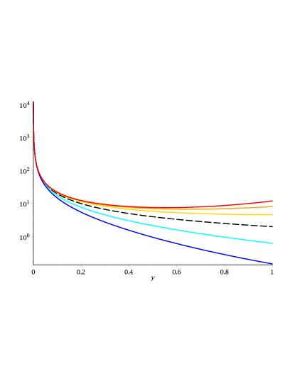
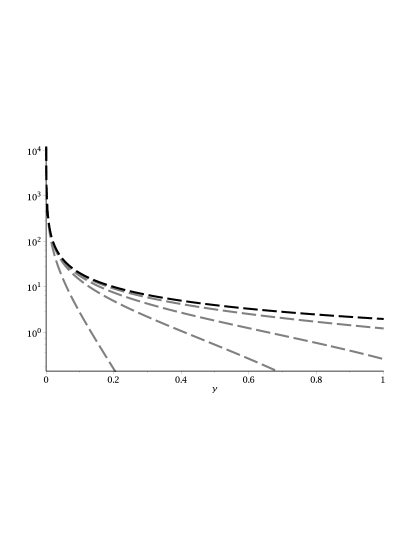
Figure 3: Left panel: the stationary AFS for six scenarios of selection, $\gamma=-2$ (blue solid line), $\gamma=-1$ (turquoise solid line), $\gamma=0$ (black dashed line), $\gamma=1$ (yellow solid line), $\gamma=2$ (orange solid line) and $\gamma=3$ (red solid line). Right panel: the build-up of the AFS starting from a completely mono-allelic state at $t=0$ for the neutral case, $\gamma=0$. The gray dashed lines represent the AFS for the time points $t=0.1$, $t=0.5$, $t=1$ and $t=2$ in increasing order. The black dashed line represents the equilibrium AFS.

To motivate the extension to the case $\mathcal{F}$ in Theorem 1, we mention $f_{\mathrm{fix}}\in\mathcal{F}$ defined by $f_{\mathrm{fix}}(y)=1_{\{y=1\}}$. Then

$$\langle\mathcal{X}_{t}^{N}\!,f_{\mathrm{fix}}\rangle=\mbox{\# of alleles that reach fixation in $[0,t]$}$$

and

$$\lim_{N\to\infty}\mathbb{E}\langle\mathcal{X}_{t}^{N}\!,f_{\mathrm{fix}}\rangle=-\theta\omega_{\gamma}\int_{0}^{1}q_{\gamma}(y)\,\mathbb{P}_{1-y}^{*\gamma}(\tau_{1}\leq t)\pi_{\gamma}(y)\,dy+\theta\omega_{\gamma}\,t.$$

But, clearly, $\int_{0}^{t\wedge\tau}f_{\mathrm{fix}}(\xi_{u})\,du=0$ and so, by (10),

$$\lim_{N\to\infty}\mathbb{E}\langle\mathcal{X}_{t}^{N}\!,f_{\mathrm{fix}}\rangle=\theta\omega_{\gamma}\,t-\theta\omega_{\gamma}\,\int_{0}^{t}\mathbb{P}^{*\gamma}_{0}(\tau_{1}>s)\,ds=\theta\omega_{\gamma}(t-\mathbb{E}^{*\gamma}_{0}(\tau_{1}\wedge t)).$$

In contrast to the work by Sawyer and Hartl [1992], who start from a stationary state, this relation, provides the precise growth in the number of fixations starting from a completely mono-allelic population at time $t=0$. Thus, it can, for example, be applied to study the number of fixations of lineage-specific mutations after a population split [Mugal et al., 2014].

3.2 Representation using the duality relationship

In this subsection, we establish an additional representation of the limit functional in Theorem 1, valid for the neutral scenario or the case of negative selection $\gamma\leq 0$. This representation of the non-equilibrium AFS results by rewriting (8), equivalently (9), using the duality between the Wright-Fisher diffusion process and a class of birth-death processes generalizing Kingman’s coalescent process. Kingman’s pure death coalescent process [Kingman, 1982], is the Markov process $(A_{t})_{t\geq 0}$ defined by jump rates

$$\mathbb{P}^{0}(A_{t+h}-A_{t}=-1|A_{t}=k)=\binom{k}{2}h+o(h),\quad h\to 0.$$ (13)

Writing $\mathbb{P}_{m}^{0}$ and $\mathbb{E}^{0}_{m}$ for the conditional law and expectation given $A_{0}=m$, Kingman’s coalescent $(A_{t})$ is a dual process of the neutral Wright-Fisher diffusion $(\xi_{t})_{t\geq 0}$, in the sense

$$\mathbb{E}^{0}_{x}(\xi_{t}^{m})=\mathbb{E}^{0}_{m}(x^{A_{t}})$$

[Tavaré, 1984], and since the distributional properties of $(A_{t})$ are known, the duality relation provides an important computational tool. Indeed, Griffiths [1979] and Tavaré [1984] showed that, under $\mathbb{P}_{m}^{0}$, the Markov transition probabilities of $A_{t}$ have the representations

$$\mathbb{P}^{0}_{m}(A_{t}=1) =1-\sum_{k=2}^{m}e^{-\binom{k}{2}t}(2k-1)(-1)^{k}\frac{m_{[k]}}{m_{(k)}}$$ (14)

$$\mathbb{P}^{0}_{m}(A_{t}=j) =\sum_{k=j}^{m}e^{-\binom{k}{2}t}\,\frac{(2k-1)(-1)^{k-j}j_{(k-1)}}{j!(k-j)!}\frac{m_{[k]}}{m_{(k)}},\quad 2\leq j\leq m,$$ (15)

with increasing and decreasing factorials defined as

$$m_{[k]}=\frac{\Gamma(m+1)}{\Gamma(m-k+1)},\quad m_{(k)}=\frac{\Gamma(m+k)}{\Gamma(m)}.$$

Furthermore,

$$\mathbb{E}^{0}_{m}(A_{t})=1+\sum_{k=2}^{m}e^{-\binom{k}{2}t}(2k-1)\frac{m_{[k]}}{m_{(k)}}.$$ (16)

These formulas remain valid as $m\to\infty$ with the replacement $m_{[k]}/m_{(k)}\to 1$, for example

$$\mathbb{E}^{0}_{\infty}(A_{t})=1+\sum_{k=2}^{\infty}e^{-\binom{k}{2}t}(2k-1).$$

The moment duality relation between the neutral Wright-Fisher diffusion process and Kingman’s coalescent process extends to duality between the Wright-Fisher diffusion process with selection and a wider class of birth-and-death processes, for which we keep the notation $A_{t}$ [Shiga and Uchiyama, 1986, Athreya and Swart, 2005]. For $\gamma\geq 0$, $(A_{t})_{t\geq 0}$ is a birth-death process with linear birth intensity $\gamma$, such that

$$\mathbb{P}(\eta_{t+h}-\eta_{t}=1|\eta_{t}=k)=\gamma kh+o(h),\quad h\to 0,$$ (17)

and death intensity the same as in (13). Then $A_{t}$ possesses a steady-state $A_{\infty}$, which has the distribution of a Poisson random variable with mean $2\gamma$, conditioned to stay positive. The duality relation is

$$\mathbb{E}^{\gamma}_{x}[(1-\xi_{t})^{m}]=\mathbb{E}^{\gamma}_{m}[(1-x)^{A_{t}}].$$

By symmetry,

$$\mathbb{E}^{-\gamma}_{x}[\xi_{t}^{m}]=\mathbb{E}^{\gamma}_{1-x}[(1-\xi_{t})^{m}].$$

Hence, if we now switch to the case $\gamma\leq 0$,

$$\mathbb{E}^{\gamma}_{1-x}[\xi_{t}^{m}]=\mathbb{E}^{-\gamma}_{m}[(1-x)^{A_{t}}].$$

This relation applied to the representation of the non-equilibrium AFS in (9) yields

$$\mathbb{P}^{\gamma}_{1-y}(\tau_{1}\leq t)=\mathbb{P}^{\gamma}_{1-y}(\xi_{t}=1)=\lim_{m\to\infty}\mathbb{E}^{\gamma}_{1-y}(\xi_{t}^{m})=\mathbb{E}^{-\gamma}_{\infty}[(1-y)^{A_{t}}]$$

so that

$$\frac{\mathbb{P}^{\gamma}_{1-y}(\tau_{1}\leq t)}{1-y}=\mathbb{E}^{-\gamma}_{\infty}[(1-y)^{A_{t}-1}]$$

and we obtain the following alternative representation of the non-equilibrium AFS in Theorem 1.

Corollary 1.

For the case of neutral evolution or negative selection, $\gamma\leq 0$, the non-equilibrium AFS in Theorem 1 has the representation

$$\omega_{\gamma}\int_{0}^{1}f(y)\,\mathbb{P}^{*\gamma}_{1-y}(\tau_{1}\leq t)\pi_{\gamma}(y)\,dy=\int_{0}^{1}\mathbb{E}^{-\gamma}_{\infty}[(1-y)^{A_{t}-1}]f(y)\,\pi_{0}(y)\,dy$$

As a remark on the computational aspects of this representation, the probabilities $\mathbb{P}^{0}_{\infty}(A_{t}=j)$ for the case $\gamma=0$ are those of (14,15) in the limit $m\to\infty$. For the negative case $\gamma<0$, one approach might be averaging over a large number of simulated paths of $(A_{t})$.

4 Population functionals and sample functionals

At this stage, we have used the discrete time Markov chain $(X_{n})$, the time-scaled allele frequencies $(X_{N}(t))$, the continuous time and continuous state scaled version $(Y_{N,L}(t))$, the random field $(\mathcal{X}_{t}^{N,L})$, and the Poisson stochastic integral $(\mathcal{X}_{t}^{N})$, to study non-equilibrium allele frequencies. Moreover, stationary versions $\mathcal{X}_{\infty}^{N}$ and $\mathcal{X}_{\infty}$ appear in the large time limit. Figure 4 shows the relation of the various random fields and the corresponding expectations. The same sequence of approximations apply to building other functionals of the allele frequencies, where it is natural to distinguish between population functionals and sample functionals. Population functionals are in principal non-observable and require knowing the history of the entire spectrum of allele frequencies in each site counted as fractions of the entire population. Sample functionals refer to the spectrum of frequencies being restricted to a smaller sample of individuals, in the sense of fixing an integer $m\geq 1$ and consider a sample of $m$ sequences chosen randomly with equal probabilities for all subsets of size $m$.

Figure 4: Schematic structure of the random fields (upper two rows), their expectations (third row) and limiting expectations (third and fourth row). Going from left to right the graph indicates the various non-equilibrium and equilibrium versions.

To identify the proper sampling functionals we consider the discrete generation version of the population model. Consider a sample of $m$ sequences. Let

$$M^{i}_{n}=\mbox{\# of sampled derived alleles in site $i$ of generation $n$}.$$

Conditionally, for each $n$ given $X_{n}$, the random variables $M_{n}^{i}$, $1\leq i\leq L$, are i.i.d. and suitably approximated by the binomial distribution Bin$(m,X^{i}_{n}/N)$. With these insights drawn from the discrete generation model it follows that $M_{[Nt]}^{i}$ is binomial with parameters $m$ and $N^{-1}X^{i}_{[Nt]}$, where the latter is a discrete approximation of $Y^{i}_{N,L}(t)$. Considering the map

$$t\mapsto\langle\mathcal{M}^{N,L}_{t}\!,g\rangle=\sum_{i=1}^{L}g(M_{N,L}^{i}(t)),\quad M_{N,L}^{i}(t)\sim\mbox{Bin}(m,Y_{N,L}^{i}(t)),$$

for $g:\mathbb{Z}\to\mathbb{R}$, $g(0)=0$, in analogy with Proposition 2 we obtain as $L\to\infty$ a limiting random field $\{\langle\mathcal{M}^{N}_{t}\!,g\rangle,\;t\geq 0\}$, such that

$$\mathcal{M}^{N}_{t}=\sum_{k=1}^{m}\delta_{Z^{N,k}_{t}}$$

and the family of random variables

$$Z^{N,k}_{t}=\mbox{\# of sites with exactly $k$ derived in the sample},\quad 1\leq k\leq m,$$

are independent and Poisson distributed with mean

$$\mathbb{E}^{\gamma}(Z_{t}^{N,k})=\theta\binom{m}{k}\,N\mathbb{E}^{\gamma}_{1/N}\Big{[}\int_{0}^{t\wedge\tau}\xi_{u}^{k}(1-\xi_{u})^{m-k}\,du\Big{]}.$$

Moreover, the sample functional $\mathcal{M}_{t}^{N}$ has a stationary version $\mathcal{M}_{\infty}^{N}$ such that the family $Z^{N,k}_{\infty}$, $1\leq k\leq m$, are independent Poisson with mean

$$\mathbb{E}^{\gamma}(Z_{\infty}^{N,k})=\theta\binom{m}{k}\,N\mathbb{E}^{\gamma}_{1/N}\Big{[}\int_{0}^{\tau}\xi_{u}^{k}(1-\xi_{u})^{m-k}\,du\Big{]}.$$

It is outside the scope of this work to study any limiting family of random processes, $\{(Z^{k}_{t})_{t\geq 0},1\leq k\leq m\}$, that might arise as $N\to\infty$. As a consequence of Theorem 1, however, we do obtain the following additional results. As $N\to\infty$, the Poisson expectations have limits

$$\mathbb{E}^{\gamma}(Z_{t}^{N,k})\to\theta\binom{m}{k}\,\omega_{\gamma}\int_{0}^{1}\mathbb{P}^{*\gamma}_{1-y}(\tau_{1}\leq t)y^{k}(1-y)^{m-k}\pi_{\gamma}(y)\,dy$$ (18)

and

$$\mathbb{E}^{\gamma}(Z_{\infty}^{N,k})\to\theta\binom{m}{k}\,\omega_{\gamma}\int_{0}^{1}y^{k}(1-y)^{m-k}\,\pi_{\gamma}(y)\,dy.$$

As an application we fix the sample size $m$ and consider

$$Z_{m}^{N}(t)=\sum_{k=1}^{m-1}Z^{N,k}_{t}=\mbox{\# of segregating sites in sample of size $m$}.$$

Using notation $a_{m}$ for the binomial formula

$$a_{m}(y)=\sum_{j=1}^{m-1}\binom{m}{j}y^{j}(1-y)^{m-j}=1-y^{m}-(1-y)^{m},\quad 0\leq y\leq 1,$$

it follows that the summation $Z_{m}^{N}(t)$ is Poisson distributed with expected value

$$\mathbb{E}^{\gamma}Z_{m}^{N}(t)=N\theta\mathbb{E}^{\gamma}_{1/N}\Big{[}\int_{0}^{t\wedge\tau}a_{m}(\xi_{u})\,du\Big{]}.$$

Since $a_{m}\in\mathcal{F}_{0}$, the limiting expected number of segregating sites,

$$S_{m}(t)=\lim_{N\to\infty}\mathbb{E}^{\gamma}Z_{m}^{N}(t),$$

is now obtained from Theorem 1 as

$$S_{m}(t)=\theta\omega_{\gamma}\int_{0}^{1}\mathbb{P}^{*\gamma}_{1-y}(\tau_{1}\leq t)a_{m}(y)\pi_{\gamma}(y)\,dy.$$

Moreover, if $\gamma\leq 0$ then by Corollary 1

$$S_{m}(t)=\theta\int_{0}^{1}E^{-\gamma}_{\infty}[(1-y)^{A_{t}-1}]\,a_{m}(y)\,\pi_{0}(y)\,dy,$$

and hence, by evaluating the integral,

$$S_{m}(t) =2\theta\,E^{-\gamma}_{\infty}\Big{[}\sum_{k=0}^{m-1}\frac{1}{k+A_{t}}-\frac{\Gamma(A_{t})\Gamma(m)}{\Gamma(A_{t}+m)}\Big{]}$$

$$\approx 2\theta E^{-\gamma}_{\infty}[\log(1+(m-1)/A_{t})].$$

Under neutral evolution $\gamma=0$, one may use (7) or (15) to obtain series representations of the limiting expressions of $S_{m}(t)$. Yet another representation of the same quantity follows from

$$\mathbb{E}^{0}Z_{m}^{N}(t) =\theta\int_{0}^{t}N\mathbb{E}^{0}_{1/N}[a_{m}(\xi_{u})]\,du$$

$$=\theta\int_{0}^{t}N\mathbb{E}_{m}^{0}[1-(1/N)^{A_{u}}-(1-1/N)^{A_{u}}]\,du$$

$$\to\theta\int_{0}^{t}(\mathbb{E}^{0}_{m}(A_{u})-\mathbb{P}^{0}_{m}(A_{u}=1))\,du,\quad N\to\infty.$$

Thus, by (14) and (16),

$$S_{m}(t)=\theta\sum_{k=2}^{m}(1+(-1)^{k})(1-e^{-\binom{k}{2}t})\frac{2k-1}{\binom{k}{2}}\frac{m_{[k]}}{m_{(k)}},$$

and we recover the fixed population size version of an expression which can be found in Tajima [1989] and Zivkovic and Stephan [2011]. For $\gamma\not=0$, the seemingly crude but straightforward approximation

$$S_{m}(t)\approx\theta\omega_{\gamma}\int_{0}^{1}\mathbb{P}^{*0}_{1-y}(\tau_{1}\leq t)a_{m}(y)\pi_{\gamma}(y)\,dy,$$ (19)

obtained by simply replacing the conditional distribution in (8) with its neutral, explicitly known, version (7), appears quite efficient and useful for many purposes. In steady-state, letting $t\to\infty$,

$$S_{m}(t)\to S_{m}=\theta\omega_{\gamma}\int_{0}^{1}a_{m}(y)\,\pi_{\gamma}(dy).$$

The neutral case $\gamma=0$ yields the familiar relation

$$S_{m}=2\theta\sum_{k=1}^{m-1}\frac{1}{k}\approx 2\theta\ln m.$$

As an illustration of these findings, Figure 5 shows the non-equilibrium growth over time of the limiting expected number of segregating sites.

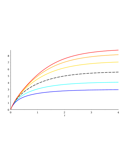
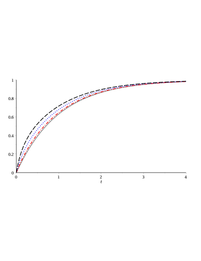
Figure 5: Left panel: the number of segregating sites, $\{S_{m}(t),0\leq t\leq 4\}$, in a sample of $m=10$ individuals, using the approximation (19), for six scenarios of selection, $\gamma=-2$ (blue solid line), $\gamma=-1$ (turquoise solid line), $\gamma=0$ (black dashed line), $\gamma=1$ (yellow solid line), $\gamma=2$ (orange solid line) and $\gamma=3$ (red solid line). Right panel: illustration of the effect of sample size for the neutral case $\gamma=0$. The normalized number of segregating sites, $\{S_{m}(t)/S_{m},0\leq t\leq 4\}$, $m=2$ (green solid line), $m=5$ (red dashed-dotted line), $m=10$ (blue dotted line), and $m=20$ (black dashed line).

5 Discussion

Several allele frequency-based summary statistics are central measurements in population genetic studies. In the study of a single population allele frequency-based measurements assist, for example, the identification of candidate loci of adaptive evolution [Tajima, 1989, Fay and Wu, 2000, Zeng et al., 2006], or the inference of the demographic history of the population [Excoffier et al., 2013]. In the study of speciation events, the consideration of the joint AFS of closely related species is of considerable interest for the underlying mechanics of speciation [Gutenkunst et al., 2009]. Moreover, measures of population differentiation, which depend on the comparison of the AFS between two populations descending from a common ancestor, are commonly used to detect genomic regions involved in the process of speciation [Seehausen et al., 2014]. From a theoretical viewpoint these kind of inferences require a sound analytical understanding of the non-equilibrium properties of the AFS as a function of time starting from any specific initial value.

Evans et al. [2007] consider the non-equilibrium AFS in a population of size $2N\rho$ with mutation rate $\theta^{\prime}$ in a bi-allelic setting with allele frequencies governed by a general class of diffusion processes, and where asymptotically in the scaling limit $N\to\infty$ the factor $\rho=\rho(t)$ may depend on time. In this setting they derive a limiting function $f(t,x)$ such that

$$f(t,x)\,dx\sim\mbox{expected fraction of alleles of frequency $[x,x+dx]$},\quad 0<x<1.$$

For the case of the Wright-Fisher diffusion process with selection parameter $S$ and varying population size $\rho(t)$, the function $f(t,x)$ is characterized by the property that the scaled function $g(t,x)=x(1-x)f(t,x)$ is a solution of

$$\frac{\partial}{\partial t}g(t,x)=-Sx(1-x)\frac{\partial}{\partial x}g(t,x)+\frac{x(1-x)}{2\rho(t)}\frac{\partial^{2}}{\partial x^{2}}g(t,x)$$

with appropriate initial value $g(0,x)=g_{0}(x)$ at $t=0$ and boundary conditions

$$\lim_{x\to 0}g(t,x)=\theta^{\prime}\rho(t),\quad\lim_{x\to 1}g(t,x)=0.$$

Comparing this result for the case $\rho(t)=1$, $S=\gamma$, $\theta^{\prime}=2\theta$ and $g_{0}=0$ with our representation (9) of the AFS in Theorem 1, leads to identifying the implicitly given function $g$ as

$$g(t,x)=2\theta\,\mathbb{P}^{\gamma}_{1-x}(\tau_{1}\leq t).$$

Similarly, using (8), one obtains the representation

$$f(t,x)=2\theta\,\mathbb{P}^{*\gamma}_{1-x}(\tau_{1}\leq t)\,\frac{1-e^{-2\gamma(1-x)}}{x(1-x)(1-e^{-2\gamma})},$$

reminding that $\mathbb{P}_{1-x}^{\gamma}$ is the probability law of the Wright-Fisher diffusion process with initial state $1-x$, $\tau_{1}$ is the time to fixation in state $1$ of the same diffusion, and $\mathbb{P}^{*\gamma}_{1-x}$ is the conditional law given $\tau_{1}<\infty$. In particular, for the neutral case $\gamma=0$,

$$f(t,x)=2\theta\,\mathbb{P}^{*0}_{1-x}(\tau_{1}\leq t)/x$$

with the probability distribution function given explicitly in (7). For non-positive selection, $\gamma\leq 0$, using the framework of duality theory of moment functionals, and recalling the birth-death process $(A_{t})$ with intensities given in (13) and (17), an alternative representation is given by

$$f(t,x)=\frac{2\theta\,\mathbb{E}^{-\gamma}[(1-x)^{A_{t}}|A_{0}\to\infty]}{x(1-x)}$$

in terms of $A_{t}$ “coming down from infinity” at time $t=0$. We thus provide exact analytical results on the non-equilibrium AFS, which if efficiently applied can improve our understanding of a broad spectrum of population genetic inferences.

Our framework can further be related to the computational method devised by Evans et al. [2007], which uses the fact that the moments

$$\mu_{n}(t)=\int_{0}^{1}x^{n}g(t,x)\,dx,\quad n=0,1,\dots$$

satisfy a coupled system of ordinary differential equations. Assuming constant population size, these moments can be identified within our framework by

$$\mu_{n}(t)=\lim_{N\to\infty}\mathbb{E}\langle\mathcal{X}_{t}^{N}\!,b_{n}\rangle,\quad b_{n}(y)=(1-y)y^{n+1}.$$

Since $b_{n}\in\mathcal{F}_{0}$, by Theorem 1,

$$\mu_{n}(t)=\theta\omega_{\gamma}\int_{0}^{1}b_{n}(y)\,\mathbb{P}^{*\gamma}_{1-y}(\tau_{1}\leq t)\pi_{\gamma}(y)\,dy.$$

Moreover, the analytical description of the build-up of the AFS starting from a completely mono-allelic state at $t=0$, can be helpful to study the build-up of lineage-specific polymorphisms as compared to the ebbing of shared ancestral polymorphisms during the process of speciation. Our work therefore ties to the work of Wakeley and Hey [1997] and Chen [2012], who model the separate AFS of lineage-specific and shared ancestral polymorphisms in samples from closely related species in the framework of coalescent theory. Precisely, our relation (18) corresponds to the AFS of lineage-specific polymorphisms in Chen [2012] (5), which in our notation reads

$$\lim_{N\to\infty}\mathbb{E}(Z_{t}^{N,k})=\theta\,\mathbb{E}^{0}_{m}\Big{[}\sum_{i=A_{t}}^{m}\frac{\binom{m-k-1}{i-2}}{\binom{m-1}{i-1}}i\,\mathbb{E}(T_{i}|A_{t})\Big{]},$$

where $T_{i}$ is the time interval during which $i$ lineages exist. While Chen [2012] provides results on the neutral AFS and the AFS in regions that underwent selective sweeps, we here add the case of negative selection. More importantly, our work illustrates that the use of the duality relation between the Wright-Fisher diffusion process and a class of birth-death processes can tie several frameworks together. We therefore foresee a broad applicability of the framework presented in this study.

6 Technical details and remaining proofs

In order to find the limits of $\mathcal{X}^{N,L}$ and $\mathcal{M}^{N,L}$ as $L\to\infty$, is is convenient to use a method first devised for Poisson random balls models [Kaj et al., 2007], which applies a set of signed measures for indexing.

6.1 Indexing random fields by measures

Let $\mathcal{H}$ be the set of finite, signed measures on the positive real line, let $|\mu|$ denote the variation norm on $\mathcal{H}$, and put

$$\mathcal{H}_{0}=\{\mu\in\mathcal{H}:\int_{0}^{\infty}|\mu|(du)<\infty\},\quad\mathcal{H}_{1}=\{\mu\in\mathcal{H}:\int_{0}^{\infty}u\,|\mu|(du)<\infty\}.$$

For a given $f\in\mathcal{F}$, denote

$$\langle\mathcal{X}^{N,L},\mu\rangle=\int\langle\mathcal{X}_{u}^{N,L}\!,f\rangle\,\mu(du)=\sum_{i=1}^{L}\int f(Y_{N,L}^{(i)}(u))\,\mu(du),\quad\mu\in\mathcal{H}_{0}.$$

In particular, with $\mu=\delta_{t}$ we have $\langle\mathcal{X}^{N,L},\delta_{t}\rangle=\langle\mathcal{X}^{N,L}_{t}\!,f\rangle$. The quantity $\langle\mathcal{M}^{N,L},\mu\rangle$ is defined analogously. Similarly, for $\mu\in\mathcal{H}$,

$$\langle\mathcal{X}^{N}\!,\mu\rangle=\int\langle\mathcal{X}_{u}^{N}\!,f\rangle\,\mu(du)=\int_{\mathbb{R}^{+}\times\mathcal{D}}\int f(\xi^{s}_{u})\,\mu(du)\,\mathcal{N}_{N}(ds,d\xi^{s}).$$

Now, in greater generality than Proposition 1, $\langle\mathcal{X}^{N}\!,\mu\rangle$ is well-defined with finite expected value, such that, for every $f\in\mathcal{F}$,

$$\mathbb{E}\langle\mathcal{X}^{N}\!,\mu\rangle=\int N\theta\,\mathbb{E}^{\gamma}_{1/N}\Big{[}\int_{0}^{u}f(\xi^{0}_{v})\,dv\Big{]}\,\mu(du)<\infty,\quad\mu\in\mathcal{H}_{1},$$ (20)

and for $f\in\mathcal{F}_{0}$,

$$\mathbb{E}\langle\mathcal{X}^{N}\!,\mu\rangle=\int N\theta\,\mathbb{E}^{\gamma}_{1/N}\Big{[}\int_{0}^{u\wedge\tau}f(\xi^{0}_{v})\,dv\Big{]}\,\mu(du)<\infty,\quad\mu\in\mathcal{H}_{0}.$$ (21)

Indeed, to verify (20) it suffices to show

$$\int_{\mathbb{R}^{+}\times\mathcal{D}}\Big{|}\int f(\xi^{s}_{u})\,\mu(du)\Big{|}\,n_{N}(ds,d\xi^{s})<\infty.$$

Here

$$\int_{\mathbb{R}^{+}\times\mathcal{D}}\int|f(\xi^{s}_{u})|\,|\mu|(du)\,n_{N}(ds,d\xi^{s}) =\mathbb{E}^{\gamma}_{1/N}\int_{0}^{\infty}\int|f(\xi^{s}_{u})|\,|\mu|(du)\,N\theta ds$$

$$=N\theta\int\mathbb{E}^{\gamma}_{1/N}\int_{0}^{\infty}|f(\xi^{s}_{u})|\,ds\,|\mu|(du),$$

and for fixed $u$,

$$\mathbb{E}^{\gamma}_{1/N}\int_{0}^{\infty}|f(\xi^{s}_{u})|\,ds=\mathbb{E}^{\gamma}_{1/N}\int_{0}^{u}|f(\xi^{s}_{u})|\,ds=\mathbb{E}^{\gamma}_{1/N}\int_{0}^{u}|f(\xi^{0}_{v})|\,dv.$$

For $f\in\mathcal{F}$ this implies

$$\int\mathbb{E}^{\gamma}_{1/N}\int_{0}^{\infty}|f(\xi^{s}_{u})|\,ds\,|\mu|(du)\leq\|f\|_{\infty}\int u\,|\mu|(du)<\infty,\quad\mu\in\mathcal{H}_{1},$$

and so

$$\mathbb{E}\langle\mathcal{X}^{f}_{N},\mu\rangle =\int_{\mathbb{R}^{+}\times\mathcal{D}}\int f(\xi^{s}_{u})\,\mu(du)\,n_{N}(ds,d\xi^{s})$$

$$=\int N\theta\,\mathbb{E}^{\gamma}_{1/N}\Big{[}\int_{0}^{u}f(\xi^{0}_{v})\,dv\Big{]}\,\mu(du),\quad\mu\in\mathcal{H}_{1}.$$

To show (21) we assume $f\in\mathcal{F}_{0}$. Then, for fixed $u$,

$$\mathbb{E}^{\gamma}_{1/N}\int_{0}^{\infty}|f(\xi^{s}_{u})|\,ds=\mathbb{E}^{\gamma}_{1/N}\int_{0}^{u\wedge\tau}|f(\xi^{0}_{v})|\,dv\leq\mathbb{E}^{\gamma}_{1/N}\int_{0}^{\tau}|f(\xi^{0}_{v})|\,dv$$

and hence using (5),

$$N\theta\int\mathbb{E}^{\gamma}_{1/N}\int_{0}^{\infty}|f(\xi^{s}_{u})|\,ds\,|\mu|(du)\leq\theta\sup_{N}N\mathbb{E}^{\gamma}_{1/N}\int_{0}^{\tau}|f(\xi^{0}_{v})|\,dv\,\int|\mu|(du)<\infty.$$

6.2 Proof of Proposition 2

To demonstrate the convergence in finite dimensional distributions of the sequence $\{\langle\mathcal{X}^{N,L}_{t}\!,f\rangle,t\geq 0\}$ to $\{\langle\mathcal{X}^{N}_{t}\!,f\rangle,t\geq 0\}$ we need to show the convergence in distribution

$$\sum_{k=1}^{n}\alpha_{k}\langle\mathcal{X}^{N,L}_{t_{k}}\!,f\rangle\stackrel{{\scriptstyle d}}{{\implies}}\sum_{k=1}^{n}\alpha_{k}\langle\mathcal{X}^{N}_{t_{k}}\!,f\rangle$$

for arbitrary weights $\alpha_{1},\dots,\alpha_{n}$ and arbitrary time points $t_{1}\leq\dots\leq t_{n}$, $n\geq 1$. But obviously, letting $\mu_{n}=\sum_{k=1}^{n}\alpha_{k}\delta_{t_{k}}$, this is the same as the convergence in distribution of $\langle\mathcal{X}^{N,L}\!,\mu_{n}\rangle$ to $\langle\mathcal{X}^{N}\!,\mu_{n}\rangle$. Because of (20) and (21) we have control of the generalized Poisson functionals in the limit and, therefore, we may continue with the method of moment generating functions. Specifically, using the defining properties of Poisson random measures,

$$\ln\mathbb{E}\exp\{\alpha\langle\mathcal{X}^{N}\!,\mu\rangle\}=N\theta\,\mathbb{E}_{1/N}^{\gamma}\Big{[}\int_{0}^{\infty}(e^{\alpha\int f(\xi^{s}_{u})\,\mu(du)}-1)\,ds\Big{]},$$

where $\mu\in\mathcal{H}_{1}$ or $\mathcal{H}_{0}$ in line with using either (20) or (21).

On the other hand, for $\mathcal{X}^{N,L}$, by the independence of the sites,

$$\ln\mathbb{E}\exp\{\alpha\langle\mathcal{X}^{N,L}\!,\mu\rangle\} =L\ln\mathbb{E}\exp\{\alpha\int f(Y^{(1)}_{N,L}(u))\,\mu(du)\}$$

$$\sim L\,\mathbb{E}\Big{[}\exp\Big{\{}\alpha\int f(Y^{(1)}_{N,L}(u))\,\mu(du)\Big{\}}-1\Big{]},$$ (22)

where we use the notation $A_{L}\sim B_{L}$ for $A_{L}/B_{L}\to 1$ as $L\to\infty$. Let $\{\kappa_{j}\}_{j\geq 1}$ be independent, exponential random variables with intensity $N\theta/L$. Since $f(0)=0$,

$$\int f(Y^{(1)}_{N,L}(u))\,\mu(du)=\int_{\kappa_{1}}^{\kappa_{1}+\tau}f(\xi_{u}^{\kappa_{1}})\,\mu(du)+\int_{\kappa_{1}+\tau+\kappa_{2}}^{\infty}f(Y^{(1)}_{N,L}(u))\,\mu(du).$$

The expected value over $\kappa_{1}$ on the right hand side in (22) now evaluates to

$$\int_{0}^{\infty}\theta Ne^{-\theta Ns/L}\mathbb{E}\Big{[}\exp\Big{\{}\alpha\int_{s}^{s+\tau}f(\xi_{u}^{s})\,\mu(du)+\alpha\int_{s+\tau+\kappa_{2}}^{\infty}\dots\,\mu(du)\Big{\}}-1\Big{]}\,ds.$$

Letting $L\to\infty$ we have $e^{-\theta Ns/L}\to 1$ and $\kappa_{2}\to\infty$, and so

$$\ln\mathbb{E}\exp\{\alpha\langle\mathcal{X}^{N,L}\!,\mu\rangle\}\to\,\int_{0}^{\infty}\theta N\mathbb{E}_{1/N}^{\gamma}\Big{[}\exp\Big{\{}\alpha\int_{s}^{s+\tau}f(\xi_{u}^{s})\,\mu(du)\Big{\}}-1\Big{]}\,ds,$$

which is the logarithmic moment generating function of $\langle\mathcal{X}^{N}\!,\mu\rangle$, hence completing the proof of convergence in distribution.

6.3 Extending Theorem 1 from $\mathcal{F}_{0}$ to $\mathcal{F}$

Our proof of Theorem 1 is stated for $f\in\mathcal{F}_{0}$, hence specifically functions $f$ with $f(1)=0$. For some applications, however, it is more natural to work with the class $\mathcal{F}$ allowing $f(1)\not=0$. To account for such cases we included two extended versions of (8) in the theorem. These follow immediately from (8) together with relations (24) and (25) of the following lemma.

Lemma 1.

Let $f$ be a bounded real-valued function defined on $[0,1]$ such that $f(0)=0$. Then

$$\mathbb{E}_{x}^{\gamma}\int_{0}^{t}f(\xi_{u})\,du=\mathbb{E}_{x}^{\gamma}\int_{0}^{t\wedge\tau}f(\xi_{u})\,du+f(1)q_{\gamma}(x)\int_{0}^{t}\mathbb{P}_{x}^{*\gamma}(\tau_{1}\leq u)\,du,$$ (23)

$$\mathbb{E}_{x}^{\gamma}\int_{0}^{t\wedge\tau}f(\xi_{u})\,du=\mathbb{E}_{x}^{\gamma}\int_{0}^{t\wedge\tau}(f(\xi_{u})-f(1)q_{\gamma}(\xi_{u}))\,du$$

$$\qquad+f(1)q_{\gamma}(x)\int_{0}^{t}\mathbb{P}_{x}^{*\gamma}(\tau_{1}>u)\,du,$$ (24)

$$\mathbb{E}_{x}^{\gamma}\int_{0}^{t}f(\xi_{u})\,du=\mathbb{E}_{x}^{\gamma}\int_{0}^{t\wedge\tau}(f(\xi_{u})-f(1)q_{\gamma}(\xi_{u}))\,du+f(1)q_{\gamma}(x)t.$$ (25)

Proof.

For bounded functions $f$ on $[0,1]$,

$$\mathbb{E}^{\gamma}_{x}\int_{0}^{t\wedge\tau}f(\xi_{r})\,dr=\int_{0}^{t}\mathbb{E}^{\gamma}_{x}[f(\xi_{r}),\tau>r]\,dr$$

and

$$\mathbb{E}^{\gamma}_{x}f(\xi_{s}) =\mathbb{E}^{\gamma}_{x}[f(\xi_{s}),\tau_{0}<s]+\mathbb{E}^{\gamma}_{x}[f(\xi_{s}),\tau_{1}<s]+\mathbb{E}^{\gamma}_{x}[f(\xi_{s}),\tau>s]$$

$$=f(0)\mathbb{P}^{\gamma}_{x}(\tau_{0}<s)+f(1)\mathbb{P}^{\gamma}_{x}(\tau_{1}<s)+\mathbb{E}^{\gamma}_{x}[f(\xi_{s}),\tau>s],$$

hence

$$\mathbb{E}_{x}^{\gamma}\int_{0}^{t} f(\xi_{u})\,du$$

$$=\mathbb{E}_{x}^{\gamma}\int_{0}^{t\wedge\tau}f(\xi_{u})\,du+f(0)\int_{0}^{t}\mathbb{P}_{x}^{\gamma}(\tau_{0}\leq u)\,du+f(1)\int_{0}^{t}\mathbb{P}_{x}^{\gamma}(\tau_{1}\leq u)\,du$$

$$=\mathbb{E}_{x}^{\gamma}\int_{0}^{t\wedge\tau}f(\xi_{u})\,du+f(0)(1-q_{\gamma}(x))+f(1)q_{\gamma}(x)t$$

$$\quad-f(0)(1-q_{\gamma}(x))\int_{0}^{t}\mathbb{P}_{x}^{*\gamma}(\tau_{0}>u)\,du-f(1)q_{\gamma}(x)\int_{0}^{t}\mathbb{P}_{x}^{*\gamma}(\tau_{1}>u)\,du.$$

Take $f(0)=0$ to obtain statement (23). Also

$$\mathbb{E}_{x}^{\gamma}\int_{0}^{t\wedge\tau}\!\!f(\xi_{u})\,du =\mathbb{E}_{x}^{\gamma}\int_{0}^{t}f(\xi_{u})\,du-f(1)q_{\gamma}(x)t+f(1)q_{\gamma}(x)\int_{0}^{t}\mathbb{P}_{x}^{*\gamma}(\tau_{1}>u)\,du.$$

Using $\mathbb{E}^{\gamma}_{x}[q_{\gamma}(\xi_{u})]=q_{\gamma}(s)$, this may be rewritten

$$\mathbb{E}_{x}^{\gamma}\int_{0}^{t\wedge\tau}f(\xi_{u})\,du =\mathbb{E}_{x}^{\gamma}\int_{0}^{t}(f(\xi_{u})-f(1)q_{\gamma}(\xi_{u}))\,du$$

$$\quad+f(1)q_{\gamma}(x)\int_{0}^{t}\mathbb{P}_{x}^{*\gamma}(\tau_{1}>u)\,du.$$

Therefore, since the function $g$ defined by $g(y)=f(y)-f(1)q_{\gamma}(y)$ satisfies $g(0)=g(1)=0$, an application of (23) to $g$ implies the second statement (24). Combine (23) and (24) to get (25). ∎

7 Acknowledgments

The authors are grateful to Hans Ellegren for encouraging this work.

References

References

• Athreya and Swart [2005] Athreya, S., Swart, J.. Branching-coalescing particle systems. Probab Theory Relat Fields 2005;131:376–414.
• Breiman [1992] Breiman, L.. Probability. SIAM: Classics in Applied Mathematics, 1992.
• Chen [2012] Chen, H.. The joint allele frequency spectrum of multiple populations: A coalescent theory approach. Theor Pop Biol 2012;81:179–195.
• Evans et al. [2007] Evans, S.E., Shvets, Y., Slatkin, M.. Non-equilibrium theory of the allele frequency spectrum. Theor Pop Biol 2007;71:109–119.
• Excoffier et al. [2013] Excoffier, L., Dupanloup, I., Huerta-Sanchez, E., Sousa, V.C., Foll, M.. Robust demographic inference from genomic and snp data. Plos Genet 2013;9.
• Fay and Wu [2000] Fay, J.C., Wu, C.I.. Hitchhiking under positive darwinian selection. Genetics 2000;155:1405–1413.
• Fisher [1930] Fisher, R.A.. The Genetical Theory of Natural Selection. Clarendon Press, Oxford, 1930.
• Fu [1995] Fu, Y.X.. Statistical properties of segregating sites. Theor Pop Biol 1995;48:172–197.
• Griffiths [1979] Griffiths, R.. On the distribution of allele frequencies in a diffusion model. Theor Pop Biol 1979;15:140–158.
• Griffiths and Tavaré [1998] Griffiths, R., Tavaré, S.. The age of a mutation in a general coalescent tree. Stochastic Models 1998;1-2:273–295.
• Gutenkunst et al. [2009] Gutenkunst, R.N., Hernandez, R.D., Williamson, S.H., Bustamante, C.D.. Inferring the joint demographic history of multiple populations from multidimensional snp frequency data. Plos Genet 2009;5.
• Kaj et al. [2007] Kaj, I., Leskelä, L., Norros, I., Schmidt, V.. Scaling limits for random fields with long-range dependence. Annals Probab 2007;35:528–550.
• Kallenberg [2002] Kallenberg, O.. Foundations of Modern Probability. Springer-Verlag, New York, 2002.
• Karlin and Taylor [1981] Karlin, S., Taylor, H.M.. A second course in stochastic processes. Academic Press, San Diego, 1981.
• Kimura [1964] Kimura, M.. Diffusion models in population genetics. J Appl Probab 1964;1:177–232.
• Kimura [1970a] Kimura, M.. The length of time required for a selectively neutral mutant to reach fixation through random frequency drift in a finite population. Genet Res 1970a;15:131–133.
• Kimura [1970b] Kimura, M.. Stochastic processes in population genetics, with special reference to distribution of gene frequencies and probability of gene fixation. In: Kojima, K.I., editor. Mathematical Topics in Population Genetics. Berlin: Springer-Verlag; 1970b. p. 178–209.
• Kingman [1982] Kingman, J.. The coalescent. Stochastic Process Appl 1982;13:235–248.
• Mugal et al. [2014] Mugal, C.F., Wolf, J.B.W., Kaj, I.. Why time matters: codon evolution and the temporal dynamics of dn/ds. Mol Biol Evol 2014;31:212–231.
• Sawyer and Hartl [1992] Sawyer, S.A., Hartl, D.L.. Population-genetics of polymorphism and divergence. Genetics 1992;132:1161–1176.
• Seehausen et al. [2014] Seehausen, O., Butlin, R.K., Keller, I., Wagner, C.E., Boughman, J.W., Hohenlohe, P.A., Peichel, C.L., Saetre, G.P., Bank, C., Brannstrom, A., Brelsford, A., Clarkson, C.S., Eroukhmanoff, F., Feder, J.L., Fischer, M.C., Foote, A.D., Franchini, P., Jiggins, C.D., Jones, F.C., Lindholm, A.K., Lucek, K., Maan, M.E., Marques, D.A., Martin, S.H., Matthews, B., Meier, J.I., Most, M., Nachman, M.W., Nonaka, E., Rennison, D.J., Schwarzer, J., Watson, E.T., Westram, A.M., Widmer, A.. Genomics and the origin of species. Nature Rev Genet 2014;15:176–192.
• Shiga and Uchiyama [1986] Shiga, T., Uchiyama, K.. Stationary states and their stability of the stepping stone model involving mutation and selection. Probab Theory Relat Fields 1986;73:87–117.
• Tajima [1989] Tajima, F.. Statistical method for testing the neutral mutation hypothesis by dna polymorphism. Genetics 1989;123:585–595.
• Tavaré [1984] Tavaré, S.. Line-of-descent and genealogical processes, and their applications in population genetics models. Theor Pop Biol 1984;26:119–164.
• Wakeley and Hey [1997] Wakeley, J., Hey, J.. Estimating ancestral population parameters. Genetics 1997;145:847–855.
• Wright [1931] Wright, S.. Evolution in mendelian populations. Genetics 1931;16:97–159.
• Wright [1938] Wright, S.. The distribution of gene frequencies under irreversible mutation. Proc Natl Acad Sci 1938;24:253–259.
• Zeng et al. [2006] Zeng, K., Fu, Y.X., Shi, S., Wu, C.I.. Statistical tests for detecting positive selection by utilizing high-frequency variants. Genetics 2006;174:1431–1439.
• Zivkovic et al. [2015] Zivkovic, D., Steinrucken, M., Song, Y.S., Stephan, W.. Transition densities and sample frequency spectra of diffusion processes with selection and variable population size. Genetics 2015;200:601–617.
• Zivkovic and Stephan [2011] Zivkovic, D., Stephan, W.. Analytical results on the neutral non-equilibrium allele frequency spectrum based on diffusion theory. Theor Pop Biol 2011;79:184–191.