MPP-2015-301 Numerical Evaluation of Two-Loop Integrals in FDR

Abstract

We present a method to numerically evaluate infrared-finite one- and two-loop integrals within the Four-Dimensional Regularization/Renormalization approach, in which a small mass serves as regulator. Typical integrals exhibit a logarithmic dependence on this mass, which we extract with the aid of suitable subtraction terms that can easily be integrated analytically until the logarithmic structure is revealed. As first physical applications to test the method, we calculate QCD corrections to the decay rates of scalar and pseudoscalar Higgs bosons into two photons in the limit of an infinite top-quark mass as well as to the $\rho$ parameter.

1 Introduction

Precise measurements at particle colliders such as the LHC necessitate theory predictions with competitive accuracy, which involve the evaluation of loop integrals. Often one needs to go beyond the one-loop level, for instance if the next-to-leading order (NLO) accuracy is not sufficient or if the leading-order (LO) diagrams are already loop-induced. While the one-loop problem is solved in principle, the calculation of two-loop integrals is in general still a major challenge with current technology. Thus any possible strategy to simplify loop calculations is highly appreciable.

The Four-Dimensional Regularization/Renormalization (FDR) approach proposed by Pittau in 2012 [1] could potentially provide a way to reduce the enormous effort required especially for next-to-next-to-leading order (NNLO) calculations [2]. In this approach an additional small mass parameter $\mu$ is introduced, maintaining gauge invariance, however, and loop integrals are redefined in a way that they are finite in four dimensions. Compared to working in Dimensional Regularization (DR) [3], which requires the evaluation of $D=(4-2\epsilon)$-dimensional integrals, this offers several simplifications. First of all the calculation of an $L$-loop observable does not require the knowledge of higher terms in the $\epsilon$ expansion of the $(L-1)$-loop result, i.e. no $\frac{\epsilon}{\epsilon}$ terms are generated. In addition, the four-dimensionality avoids problems regarding the continuation of $\gamma_{5}$ to $D$ dimensions and, in principle, welcomes numerical approaches. Another advantage of FDR is that infrared (IR) divergencies are regulated at the same time, which was demonstrated to work at NLO using a small gluon mass in the phase-space integration [4] but still needs to be explored for higher orders [5]. For IR-finite observables, to which we will restrict ourselves in this paper, complete one-loop [6, 7, 8] and two-loop [2] calculations have been performed finding agreement with DR results.

Whereas the computations mentioned above were performed analytically, we will pursue a numerical approach in this paper. For dimensionally-regulated integrals it is absolutely necessary to expand in the regulator $\epsilon$ before the numerical integration can be performed. This can be achieved (at one-loop order) using local subtraction terms in loop momentum space [9] or (at in principle arbitrary loop order) in Feynman parameter space using sector decomposition [10, 11], for example. For FDR integrals, however, the divergencies merely lead to a logarithmic dependence on the regulator $\mu$. If the expected asymptotic behavior is known, one could in principle try to evaluate the integrals directly for small values of $\mu$, subtract the corresponding logarithmic terms from the result, and extrapolate to $\mu=0$. Nevertheless, this would lead to sharply peaked integrands that are difficult to evaluate numerically. An expansion in the regulator on the integrand level is thus very helpful, although not strictly necessary. A possible way to find suitable local subtraction terms on the level of Feynman parameters is the main topic of this paper.

The structure of the rest of this paper is the following: In Section 2 we present our idea how to construct subtraction terms on the level of Feynman parameters, essentially by partly linearizing the denominator. Some physical applications of this idea are shown in Section 3 before we give our conclusions in Section 4.

2 Formalism

We begin this section with a brief review of the definition of the FDR integral [1] in Section 2.1 before we elaborate on our approach to construct subtraction terms for the one and two-loop cases in Section 2.2.

2.1 The FDR Integral

Consider a dimensionally regulated, IR-finite $L$-loop integral

$$\mathcal{I}^{\text{DR}}=\mu_{R}^{2\epsilon L}\prod_{k=1}^{L}\int\mathrm{d}^{D}l_{k}\,J(\{l_{i},q_{i},m_{i}\},\epsilon),$$ (1)

where $q_{i}$ and $m_{i}$ denote external momenta and internal masses, respectively, and $D=4-2\epsilon$. The FDR interpretation of such an integral is based on a splitting of the integrand of the form

$$J=\lim_{\mu\to 0}\left[J_{V}+J_{F}\right],$$ (2)

where a new scale $\mu$ is introduced, which is required to be lower than all the other scales in the problem and will be identified with the renormalization scale later. The splitting is defined in such a way that $J_{V}$ sums up the contributions from divergent vacuum configurations, which are assumed to be unphysical. Consequently, $J_{F}$ must contain all the information on the physical process and, since it is free of UV divergencies, it can be calculated in four dimensions.

The divergent vacuum integrals contained in the integral over $J_{V}$ depend only on $\mu$, so they either yield contributions proportional to powers of $\mu^{2}$, which vanish in the asymptotic limit $\mu\to 0$, constant terms, or logarithms of the form $\ln^{k}\left(\frac{\mu^{2}}{\mu_{R}^{2}}\right)$, $k\in\{1,2,\cdots,L\}$. The latter can be eliminated by setting $\mu=\mu_{R}$. Thus, if the FDR integral is defined as

$$\mathcal{I}^{\text{FDR}} \equiv\lim_{\mu\rightarrow 0}\prod_{k=1}^{L}\int\mathrm{d}^{4}l_{k}\,J_{F}(\{l_{i},q_{i},m_{i}\},\mu)\bigg{|}_{\mu=\mu_{R}}$$

$$=\mathcal{I}^{\text{DR}}-\lim_{\mu\rightarrow 0}\prod_{k=1}^{L}\int\mathrm{d}^{D}l_{k}\,J_{V}(\{l_{i}\},\mu,\epsilon)\bigg{|}_{\mu=\mu_{R}},$$ (3)

the difference between $\mathcal{I}^{\text{FDR}}$ and $\mathcal{I}^{\text{DR}}$ is a ($\epsilon$-dependent) constant.

To construct the splitting into $J_{F}$ and $J_{V}$ the prescription is to replace the loop momentum in every propagator by $l_{i}^{2}\to l_{i}^{2}-\mu^{2}\equiv\overline{l_{i}}^{2}$^, and to apply the partial-fraction relations

$$\frac{1}{\overline{l_{i}}^{2}-m_{j}^{2}} =\frac{1}{\overline{l}^{2}_{i}}\left(1+\frac{m_{j}^{2}}{\overline{l}^{2}_{i}-m_{j}^{2}}\right),$$ (4a)

$$\frac{1}{\overline{(l_{i}+q_{j})}^{2}-m_{j}^{2}} =\frac{1}{\overline{l}^{2}_{i}}\left(1+\frac{m_{j}^{2}-q_{j}^{2}-2l_{i}\cdot q_{j}}{\overline{(l_{i}+q_{j})}^{2}-m_{j}^{2}}\right)$$ (4b)

repeatedly to the integrand, until all the terms are either divergent vacuum integrals or UV-finite. The former can be identified as part of $J_{V}$ and be dropped, the latter as part of $J_{F}$ and be evaluated in four dimensions. In this way, the UV divergencies contained in $\mathcal{I}^{\text{DR}}$ are traded in for IR divergencies related to vanishing $\mu$.

For gauge theories it is essential that the rules $l_{i}^{2}\to\overline{l_{i}}^{2}$ are applied to the numerator as well so that the additional mass scale $\mu$ does not spoil gauge invariance. In addition, the $\mu^{2}$ piece has to be treated exactly as the corresponding $l_{i}^{2}$ term until all UV divergencies are subtracted, i.e. one should distinguish different $\mu_{i}^{2}$ and count them as $l_{i}^{2}$ when deciding by power counting how often Eq. (4) has to be applied. In this way, gauge symmetry is preserved. The purpose of this is to ensure that FDR and DR results are related in a consistent and universal way. They are connected by finite renormalization constants [2, 5], like results obtained in different renormalization schemes.

Tensor reduction is allowed in FDR as well and can be performed in four dimensions, which generates fewer terms. However, the resulting factors of $l_{i}^{2}$ are not to be interpreted as $l_{i}^{2}-\mu_{i}^{2}$ and can thus be canceled against suitable propagators only at the price of introducing $\mu_{i}^{2}$ terms in the numerator. Such terms can give finite contributions and must be treated carefully.

2.2 Construction of the Subtraction Terms

2.2.1 General Structure in Feynman Parameter Representation

After isolating and subtracting the UV divergencies, an $L$-loop FDR integral typically has the form

$$\mathcal{I} =\prod_{j=1}^{L}\int\mathrm{d}^{4}l_{j}\,N\left(\{l_{i},q_{i},m_{i}\},\mu^{2}\right)\cdot\prod_{k=1}^{N_{x}}D^{\alpha_{k}}(p_{k},q_{k},m_{k})\cdot\prod_{n=1}^{N_{y}}D_{0}^{\beta_{n}}(p_{n}),\quad\alpha_{i},\beta_{i}\in\mathds{N},$$ (5)

where $p_{i}$ and $q_{i}$ are linear combinations of the loop and external momenta, respectively, and we distinguish two types of propagators:

$$D^{-1}(p,q,m) =(p+q)^{2}-m^{2}-\mu^{2}+i\varepsilon,$$ (6a)

$$D^{-1}_{0}(p) =p^{2}-\mu^{2}+i\varepsilon.$$ (6b)

We restrict ourselves to cases where one can find a momentum routing such that $q_{i}^{2}\neq m_{i}^{2}$ for all $i$, i.e. we assume sufficiently good IR behavior. The IR regime is then governed entirely by the $D_{0}$-type propagators, which are generated in heaps from applying the partial fraction relations (4) but may also originate from massless lines of the graph under consideration. Furthermore, $N$ denotes a non-trivial numerator including scalar products of loop and external momenta as well as powers of $\mu^{2}$.

Since we exclude IR divergencies, the integral will have an asymptotic small-$\mu^{2}$ behavior of the form

$$\mathcal{I}=\sum_{i=0}^{L}A_{i}\ln^{i}\left(\mu^{2}\right)+\mathcal{O}\left(\mu^{2}\right).$$ (7)

The $\mathcal{O}\left(\mu^{2}\right)$ terms should be dropped according to the definition of the FDR integral (2.1) so we are interested only in the logarithmic behavior for $\mu^{2}\to 0$, i.e. in the coefficients $A_{0},\cdots,A_{L}$.

In order to find the origin of the divergencies that occur in this limit, it turns out to be useful to introduce Feynman parameters first. As we will see, in Feynman parameter space one can construct simpler integrals that possess the same small-$\mu^{2}$ behavior as the original integral and can serve as local subtraction terms. These auxiliary integrands can be integrated analytically over at least a subset of the parameters so that their logarithmic dependence on $\mu^{2}$ becomes explicit. The remaining integrations can then be performed numerically.

Denoting the Feynman parameters for the two classes of propagators defined in Eq. (6) $x_{i}$ and $y_{i}$, respectively, one obtains integrals of the form

$$\mathcal{I} =\prod_{i=1}^{N_{x}}\int_{0}^{1}\mathrm{d}x_{i}\,\prod_{j=1}^{N_{y}}\int_{0}^{1}\mathrm{d}y_{j}\,\,\delta\left(1-\sum_{k=1}^{N_{x}}x_{k}-\sum_{l=1}^{N_{y}}y_{l}\right)$$

$$\quad\cdot\frac{p(x_{1},\cdots,x_{N_{x}},y_{1},\cdots,y_{N_{y}})}{\left(b^{T}\operatorname{adj}(A)b+\det(A)c\right)^{N_{1}}\det(A)^{N_{2}}}.$$ (8)

The $L\times L$ matrix $A$, the $L$-dimensional vector $b$, and the scalar $c$ are obtained by expressing the sum of all propagators in terms of the loop momenta $l=(l_{1},\cdots,l_{L})$:

$$\sum_{j=1}^{N_{x}}D(p_{j},q_{j},m_{j})+\sum_{k=1}^{N_{y}}D_{0}(p_{k}) =l^{T}Al+2b\cdot l-c.$$ (9)

The elements of $A$ are sums of $x_{i}$ and $y_{i}$ parameters, $b$ contains terms of the form $x_{i}q_{i}$, and $c$ reads

$$c =\sum_{i=1}^{N_{x}}x_{i}(m_{i}^{2}-q_{i}^{2})+\mu^{2}-i\varepsilon.$$ (10)

$p$ is a polynomial whose coefficients depend on the kinematic invariants and is a result of higher powers of propagators as well as possible non-trivial denominators. One way to treat the latter is to interpret them as inverse propagators and to calculate the derivative with respect to the corresponding Feynman parameter rather than integrating over it [13].

If we ask which region in parameter space the logarithmic divergencies regulated by $\mu$ originate from, it must be the region where the denominator of Eq. (2.2.1) is of order $\mu^{2}$. Note that the only place where $\mu^{2}$ enters the denominator is $c$. Assuming $q_{i}^{2}<m_{i}^{2}$ for all $i$, it follows that all the $x_{i}$ need to be small in order to make the denominator of order $\mu^{2}$. The term $b^{T}\operatorname{adj}(A)b$ vanishes as well in this limit, so that indeed $b^{T}\operatorname{adj}(A)b+\det(A)c\propto\mu^{2}$.

A potential problem arises if $\det(A)$ vanishes as well. In a more detailed analysis, one finds that this produces overlapping singularities that need to be disentangled. After discussing in brief the one-loop case, where this problem is absent, we will show how this can be resolved for the case $L=2$.

2.2.2 Subtraction Terms for the One-Loop Case

For $L=1$ a major simplification occurs: It is $\det(A)=\sum_{i=1}^{N_{x}}x_{i}+\sum_{i=1}^{N_{y}}y_{i}=1$, which obviously never vanishes. In addition, there is only one $y$ parameter, which we integrate out using the delta function to obtain

$$\mathcal{I}^{(1l)} =\prod_{i=1}^{N_{x}}\int_{0}^{1}\mathrm{d}x_{i}\,\,\theta\left(1-\sum_{k=1}^{N_{x}}x_{k}\right)\frac{p\left(x_{1},\cdots,x_{N_{x}},1-\sum_{k=1}^{N_{x}}x_{k}\right)}{\left(\mu^{2}+\sum_{j=1}^{N_{x}}x_{j}(m_{j}^{2}-q_{j}^{2})+\left(\sum_{j=1}^{N_{x}}x_{j}q_{j}\right)^{2}\right)^{N_{1}}}.$$ (11)

As pointed out above, the region of interest is where all $x_{i}$ go to zero. Applying the useful relation

$$\prod_{i=1}^{n}\int_{0}^{1}\mathrm{d}x_{i}\,\,\theta\left(1-\sum_{k=1}^{n}x_{k}\right)f(x_{1},\cdots,x_{n})$$

$$= \prod_{i=1}^{n}\int_{0}^{1}\mathrm{d}x_{i}\,\,\delta\left(1-\sum_{k=1}^{n}x_{k}\right)\int_{0}^{1}\mathrm{d}r\,r^{n-1}f(rx_{1},\cdots,rx_{n}),$$ (12)

one can achieve that this region is associated with the vanishing of only one parameter, namely $r$:

$$\mathcal{I}^{(1l)} =\prod_{i=1}^{N_{x}}\int_{0}^{1}\mathrm{d}x_{i}\,\,\delta\left(1-\sum_{k=1}^{N_{x}}x_{k}\right)\int_{0}^{1}\mathrm{d}r\,r^{N_{x}-1}$$

$$\quad\cdot\frac{p\left(rx_{1},\cdots,rx_{N_{x}},1-r\right)}{\left(\mu^{2}+r\sum_{j=1}^{N_{x}}x_{j}(m_{j}^{2}-q_{j}^{2})+r^{2}\left(\sum_{j=1}^{N_{x}}x_{j}q_{j}\right)^{2}\right)^{N_{1}}}$$ (13)

Now we are ready to construct an auxiliary integrand that is easier to integrate but has the correct dependence on $\ln(\mu^{2})$. For this purpose, we rewrite Eq. (2.2.2) as

$$\mathcal{I}^{(1l)} =\frac{1}{(M^{2})^{N_{1}}}\prod_{i=1}^{N_{x}}\int_{0}^{1}\mathrm{d}x_{i}\,\,\delta\left(1-\sum_{k=1}^{N_{x}}x_{k}\right)\int_{0}^{1}\mathrm{d}r\,\tilde{p}(x_{1},\cdots,x_{N_{x}},r)$$

$$\quad\cdot I_{1}^{(N_{1},n_{1},n_{2},n_{3})}\left(\frac{\mu^{2}}{M^{2}},\frac{\sum_{j=1}^{N_{x}}x_{j}(m_{j}^{2}-q_{j}^{2})}{M^{2}},\frac{\left(\sum_{j=1}^{N_{x}}x_{j}q_{j}\right)^{2}}{M^{2}};r\right),$$ (14)

where we have introduced a generic notation for the integrand,

$$I_{1}^{(N_{1},n_{1},n_{2},n_{3})}(a,c_{1},c_{2};r)\equiv\frac{r^{N_{1}-1+n_{1}}(1-r)^{n_{2}}a^{n_{3}}}{(a+c_{1}r+c_{2}r^{2})^{N_{1}}},$$ (15)

and factorized as many factors of $r$,$(1-r)$, and $a$ from $p$ so that the remainder $\tilde{p}$ is still a polynomial.

The behavior for small $\mu^{2}$ is now completely determined by the parameters of $I_{1}$. In the case $n_{1}=n_{3}=0$, for example, there will be a logarithmic dependence on $\mu^{2}$. We observe that the coefficient of $\ln(\mu^{2})$ does not depend on $c_{2}$, i.e. stetting $c_{2}=0$ would alter only the finite term. Similarly, $n_{2}$ and the $r$ dependence of $\tilde{p}$ do not influence the logarithm. Thus it suffices to calculate the auxiliary integral

$$\mathcal{A}^{(1l)} \equiv\frac{1}{(M^{2})^{N_{1}}}\prod_{i=1}^{N_{x}}\int_{0}^{1}\mathrm{d}x_{i}\,\,\delta\left(1-\sum_{k=1}^{N_{x}}x_{k}\right)$$

$$\quad\cdot\int_{0}^{1}\mathrm{d}r\,I_{1}^{(N_{1},0,0,0)}\left(\frac{\mu^{2}}{M^{2}},\frac{\sum_{j=1}^{N_{x}}x_{j}(m_{j}^{2}-q_{j}^{2})}{M^{2}},0;r\right)\tilde{p}(x_{1},\cdots,x_{N_{x}},0),$$ (16)

in order to reproduce the correct $\mu^{2}$ dependence in this case. The denominator is now linear in $r$, which is the decisive simplification. To get the correct finite part one now only has to calculate

$$\lim_{\mu\to 0}\mathcal{R}^{(1l)} \equiv\lim_{\mu\to 0}\left\{\mathcal{I}^{(1l)}-\mathcal{A}^{(1l)}\right\}$$

$$=\frac{1}{(M^{2})^{N_{1}}}\prod_{i=1}^{N_{x}}\int_{0}^{1}\mathrm{d}x_{i}\,\,\delta\left(1-\sum_{k=1}^{N_{x}}x_{k}\right)\int_{0}^{1}\mathrm{d}r\,$$

$$\quad\cdot\left\{I_{1}^{(N_{1},n_{1},n_{2},n_{3})}\left(0,\frac{\sum_{j=1}^{N_{x}}x_{j}(m_{j}^{2}-q_{j}^{2})}{M^{2}},\frac{\left(\sum_{j=1}^{N_{x}}x_{j}q_{j}\right)^{2}}{M^{2}};r\right)\tilde{p}(x_{1},\cdots,x_{N_{x}},r)\right.$$

$$\qquad\left.-I_{1}^{(N_{1},0,0,0)}\left(0,\frac{\sum_{j=1}^{N_{x}}x_{j}(m_{j}^{2}-q_{j}^{2})}{M^{2}},0;r\right)\tilde{p}(x_{1},\cdots,x_{N_{x}},0)\right\},$$ (17)

where we were able to interchange the limit $\mu\to 0$ with the integration because the integrand is well-behaved in the region of small $r$ by construction. Thus the evaluation of the difference can be done completely numerically if necessary.

2.2.3 Subtraction Terms for the Two-Loop Case

In the case $L=2$, one can label the momenta in such a way that each propagator contains either $l_{1}$, $l_{2}$, or $l_{12}\equiv l_{1}+l_{2}$. We will distinguish three subclasses of propagators, depending on which of the three momenta they contain. For the $D$-type propagators (cf. Eq. (6)) we introduce three disjoint index sets $\mathcal{X}_{1}$, $\mathcal{X}_{2}$, and $\mathcal{X}_{12}$ with the following property: If a propagator contains $l_{i}$ ($i\in\{1,2,12\}$), the index of its Feynman parameter will be an element of $\mathcal{X}_{i}$. Since the $D_{0}$-type propagators are uniquely determined by the loop momentum, we can simply define the parameter of $\frac{1}{l_{i}^{2}-\mu^{2}}$ to be $y_{i}$ for $i\in\{1,2,12\}$.

Using these conventions and assuming that the integral under consideration contains at least one $D$ and one $D_{0}$ propagator with each $l_{i}$, one can verify easily that

$$\det(A) =a_{1}a_{2}+a_{1}a_{12}+a_{2}a_{12},$$ (18a)

$$b^{T}\operatorname{adj}(A)b =a_{12}(b_{1}-b_{2})^{2}+a_{2}(b_{1}+b_{12})^{2}+a_{1}(b_{2}+b_{12})^{2},$$ (18b)

where

$$a_{i}=y_{i}+\sum_{k\in\mathcal{X}_{i}}x_{k},\quad b_{i}=\sum_{k\in\mathcal{X}_{i}}x_{k}q_{k},\quad i\in\{1,2,12\}.$$ (19)

Now it is crucial to understand when a zero of $\det(A)$ overlaps with the region we are interested in, i.e. where all $x_{i}$ are small. Since it is

$$a_{1}+a_{2}+a_{12}=y_{1}+y_{2}+y_{12}+\sum_{i=1}^{N_{x}}x_{i}=1$$ (20)

due to the delta function, the point $a_{1}=a_{2}=a_{12}=0$ is outside the integration boundaries. Thus only the zeros at $(a_{1},a_{2},a_{12})=(1,0,0),(0,1,0),(0,0,1)$ remain, which, in view of Eq. (19), are associated with zeros of either $y_{1}$, $y_{2}$, or $y_{12}$. It turns out to be sufficient to factorize the worst-behaved zero. Consider a typical structure that will lead to a logarithmic dependence on $\mu^{2}$:

$$\frac{1}{\overline{l_{1}}^{4}\overline{l_{2}}^{2}\overline{l_{12}}^{2}}$$ (21)

Since the propagator $\frac{1}{\overline{l_{1}}^{2}}$ is squared, its parameter $y_{1}$ will appear as an extra factor in the numerator. Thus the behavior at $a_{1}=1$ is worst because in the other cases this extra factor becomes small and partly compensates the vanishing of the denominator.

The next step is to find a parametrization that not only factorizes the worst zero of $\det(A)$ but also makes it possible to judge which terms can be neglected in an easy-to-integrate auxiliary integrand. It is convenient to eliminate the parameter of the $D_{0}$-type propagator with the highest power, which, like in the example above, we assume to be $y_{1}$ in the following. To parametrize the zero of $\det(A)$ and the simultaneous vanishing of the $x_{i}$ in terms of a smaller set of parameters, we make use of the following transformation, which corresponds to applying Eq. (2.2.2) three times to different subsets of parameters:

$$x_{i} \rightarrow(1-r)tx_{i} \quad i\in\mathcal{X}_{1},$$ (22a)

$$x_{i} \rightarrow rsx_{i} \quad i\in\mathcal{X}_{2}\cup\mathcal{X}_{12},$$ (22b)

$$y_{1} \rightarrow(1-r)(1-t),$$ (22c)

$$y_{i} \rightarrow r(1-s)y_{i} \quad i\in\{2,12\}.$$ (22d)

The limit $(a_{1},a_{2},a_{12})\to(1,0,0)$ is mapped to $r\to 0$, and a factor of $r$ can be split off from $\det(A)$ and also from the complete denominator.

Application of this transformation to Eq. (2.2.1) (reduced to $L=2$ and $N_{y}=3$) yields

$$\mathcal{I}^{(2l)} =\prod_{i=1}^{N_{x}}\int_{0}^{1}\mathrm{d}x_{i}\,\,\delta\left(1-\sum_{l\in\mathcal{X}_{1}}x_{l}\right)\,\delta\left(1-\sum_{m\in\mathcal{X}_{2}\cup\mathcal{X}_{12}}x_{m}\right)$$

$$\quad\cdot\int_{0}^{1}\mathrm{d}y_{2}\,\int_{0}^{1}\mathrm{d}y_{12}\,\,\delta\left(1-y_{2}-y_{12}\right)\int_{0}^{1}\mathrm{d}r\,\int_{0}^{1}\mathrm{d}s\,\int_{0}^{1}\mathrm{d}t\,I_{2}^{(N_{1},N_{2})}(r,s,t),$$ (23)

where again the behavior for small $\mu^{2}$ is determined by an integral over fewer parameters, namely

$$I_{2}^{(N_{1},N_{2})}(r,s,t)$$

$$\equiv\frac{\tilde{p}(x_{1},\cdots,x_{N_{x}},y_{2},y_{12},r,s,t)}{\left[\left(1-r+r\,d(s)\right)\left(\mu^{2}+c_{1}rs+c_{2}(1-r)t\right)+e(r,s,t)\right]^{N_{1}}\left(1-r+r\,d(s)\right)^{N_{2}}}.$$ (24)

The coefficients

$$c_{1} =\sum_{k\in\mathcal{X}_{2}\cup\mathcal{X}_{12}}x_{k}(m_{k}^{2}-q_{k}^{2}),$$ (25a)

$$c_{2} =\sum_{k\in\mathcal{X}_{1}}x_{k}(m_{k}^{2}-q_{k}^{2})$$ (25b)

are constants with respect to $r$, $s$, and $t$, whereas $d$ and $e$ are polynomials in these variables:

$$\,d(s) =a_{2}(s)a_{12}(s),$$ (26a)

$$\,e(r,s,t) =(1-r)^{2}t^{2}b_{1}^{2}+2rs(1-r)t\left[a_{2}(s)b_{12}-a_{12}(s)b_{2}\right]\cdot b_{1}$$

$$\quad+r^{2}s^{2}\left[a_{2}(s)b_{12}^{2}+a_{12}(s)b_{2}^{2}\right]+rs^{2}(1-r)(b_{2}+b_{12})^{2},$$ (26b)

where $b_{i}$, $i\in\{1,2,12\}$ as in Eq. (19) and

$$a_{2}(s) =(1-s)y_{2}+s\sum_{k\in\mathcal{X}_{2}}x_{k},$$ (27a)

$$a_{12}(s) =(1-s)y_{12}+s\sum_{k\in\mathcal{X}_{12}}x_{k}.$$ (27b)

Taking a closer look at Eq. (2.2.3), we see that the denominator is dominated by $\mu^{2}$ if $rs$ and $(1-r)t$ both vanish, i.e. the logarithmic dependence is associated with three parameters. In the limit $r\to 1$, which in view of Eqs. (19) and (22) corresponds to $a_{1}\to 0$, the integrand should be integrable because we required the worst, i.e. logarithmic divergency to be at $a_{1}\to 1$. The balance between numerator and denominator both vanishing in this limit will still be present after the transformation of variables.

To eventually construct the auxiliary integrand, we replace the denominator

$$D=\left(1-r+r\,d(s)\right)\left(\mu^{2}+c_{1}rs+c_{2}(1-r)t\right)+e(r,s,t)$$ (28)

by

$$\tilde{D} =\left(1-r+r\,d(0)\right)\left(\mu^{2}+c_{1}rs+c_{2}(1-r)t+rs^{2}(b_{2}+b_{3})^{2}\right)$$ (29)

$$=D+\mathcal{O}\left(rs\mu^{2},r^{2}s^{2},rs(1-r)t,(1-r)^{2}t^{2}\right).$$ (30)

In the numerator one should drop terms of $\mathcal{O}\left(rs\mu^{2},r^{2}s^{2},rs(1-r)t,(1-r)^{2}t^{2}\right)$ as well, but this must be done in such a way that the behavior in the limit $r\to 1$ is not spoilt.

The subtraction and evaluation of the integrals can be performed analogously to the one-loop case except that the integrations over $r$,$s$, and $t$ of the auxiliary integral must be performed analytically.

3 Applications

To test our approach for the one-loop case, one can simply calculate single integrals and compare to $\overline{\text{MS}}$-renormalized results, taking into account a possible finite part of the subtracted vacuum integral. At the two-loop level, however, this one-to-one correspondence between FDR and DR integrals is lost [2]. Thus we are forced to calculate physical observables in order to be able to compare to DR results.

For this purpose we choose NLO QCD corrections to the decay rate of scalar and pseudoscalar Higgs bosons into two photons in the heavy-top limit and to the $\rho$ parameter. Both quantities can be calculated with external momenta set to zero, i.e. only vacuum integrals need to be evaluated. Amongst other simplifications, this has the advantage that no thresholds or pseudo-thresholds will be present so we do not need to perform any analytic continuation or contour deformation in this first test of our method.

Before presenting results for these observables in Sections 3.2 and 3.3, we briefly describe the setup of the calculation.

3.1 Setup

In order to generate the amplitudes related to the observables we wish to compute, we make use of the following tools:

• qgraf [16] for the generation of the diagrams,

• q2e/exp [17, 18] for topology matching, performing the asymptotic expansion [19, 20] in small external momenta and inserting the Feynman rules, and, where necessary,

• MATAD [21] to evaluate the vacuum integrals in DR for comparison.

The next step is to interpret the integrals in the amplitude within the FDR approach and derive the splitting into divergent and finite contributions, which is done in an automated way in FORM [22, 23, 24] by systematic power counting and repeated application of Eq. (4). Our FORM routines also introduce Feynman parameters and express the result in terms of integrals of the type shown in Eqs. (15) and (2.2.3). Factors involving the loop momentum in the numerator are taken into account by calculating derivatives of intermediate Schwinger parameters [13], where the derivatives are performed algebraically, i.e. using relations of the type $\left[\frac{\partial}{\partial x},f(x)\right]=f^{\prime}(x)$.

Then we switch to Mathematica, which is used to evaluate the required auxiliary integrals case by case for a given set of exponents, and write out the amplitude in terms of functions of the remaining variables as c++ code. To perform the numerical integrations we make use of the CUBA library [25], where we choose the deterministic Cuhre algorithm [26], which turns out to perform best for the type of functions that occur in our approach, at least in absence of thresholds. To optimize the computation time we adjust the required precision for the individual integrals dynamically depending on their contribution to the final result.

3.2 Higgs Decay into Two Photons at $\mathcal{O}\left(\alpha\alpha_{S}\right)$

The decay of a Higgs boson into two photons in the limit of an infinite top-quark mass already served as a test example for FDR at the two-loop level in Ref. [2], where agreement with the DR result [27, 28] was found. We will reproduce this result with our method and supplement it with the case of a pseudoscalar Higgs boson, which is of particular interest because it is linked to the axial anomaly [29], as explained in Ref. [30].

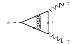
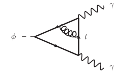
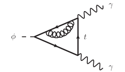
Figure 1: Two-loop QCD corrections to $\phi\rightarrow\gamma\gamma$, $\phi\in\{h,A\}$.

In terms of the momenta $q_{1,2}$ and the polarization vectors $\epsilon_{1,2}$ of the photons the amplitude for the decay of a scalar (pseudoscalar) Higgs boson $h$ ($A$) can be written as

$$\mathcal{M}_{h\rightarrow\gamma\gamma} =\left(\mathcal{M}_{h,t}+\mathcal{M}_{h,b}+\mathcal{M}_{h,W}\right)\left(q_{1}\cdot q_{2}\,\varepsilon_{1}\cdot\varepsilon_{2}-q_{1}\cdot\varepsilon_{2}\,q_{2}\cdot\varepsilon_{1}\right)\;\text{or}$$ (31a)

$$\mathcal{M}_{A\rightarrow\gamma\gamma} =\left(\mathcal{M}_{A,t}+\mathcal{M}_{A,b}\right)\epsilon_{\mu\nu\rho\sigma}q_{1}^{\mu}q_{2}^{\nu}\varepsilon_{1}^{\rho}\varepsilon_{2}^{\sigma},$$ (31b)

respectively, and in general receives contributions from heavy quarks and, in the scalar case, $W$ bosons. Here we consider only NLO QCD corrections to the top-loop contribution,

$$\mathcal{M}_{\phi,t}=\mathcal{M}_{\phi,t}^{(0)}+\frac{\alpha_{S}}{\pi}\mathcal{M}_{\phi,t}^{(1)}+\mathcal{O}\left(\alpha_{S}^{2}\right),\quad\phi\in\{h,A\},$$ (32)

for which typical diagrams are shown in Fig. 1.

Writing the top-quark couplings to the Higgs bosons generically as

$$\langle ht_{i}\bar{t}_{j}\rangle: \quad ig_{ht\bar{t}}\frac{M_{t}^{\text{bare}}}{v}\delta_{ij},$$ (33a)

$$\langle At_{i}\bar{t}_{j}\rangle: \quad ig_{At\bar{t}}\frac{M_{t}^{\text{bare}}}{v}\gamma_{5}\delta_{ij},$$ (33b)

the renormalized DR amplitudes read

$$\mathcal{M}_{h,t}(M_{t}\to\infty) =-2\frac{\alpha}{\pi}Q_{t}^{2}\frac{g_{ht\bar{t}}}{v}\left(1-\frac{\alpha_{S}}{\pi}+\mathcal{O}\left(\alpha_{S}^{2}\right)\right),$$ (34a)

$$\mathcal{M}_{A,t}(M_{t}\to\infty) =-3i\frac{\alpha}{\pi}Q_{t}^{2}\frac{g_{At\bar{t}}}{v}\left(1+\mathcal{O}\left(\alpha_{S}^{2}\right)\right).$$ (34b)

With the setup described in the previous section we obtain in FDR (without any renormalization necessary)

$$\frac{\mathcal{M}_{h,t}^{(1)}(M_{t}\to\infty)}{\mathcal{M}_{h,t}^{(0)}(M_{t}\to\infty)} =(1.9\pm 3.3)\cdot 10^{-6}\frac{M_{t}^{2}}{s}-\left\{1+(2.7\pm 0.7)\cdot 10^{-6}\right\},$$ (35a)

$$\frac{\mathcal{M}_{A,t}^{(1)}(M_{t}\to\infty)}{\mathcal{M}_{A,t}^{(0)}(M_{t}\to\infty)} =(0.1\pm 0.8)\cdot 10^{-6},$$ (35b)

i.e. we find numerical agreement to the level of $10^{-6}$. Note that in contrast to DR the usage of $\gamma_{5}$ is unproblematic in FDR. In the calculation of Eq. (35b) we simply evaluated the fermion trace in four dimensions.

3.3 Corrections to the $\rho$ Parameter at $\mathcal{O}\left(G_{F}\alpha_{S}\right)$

     

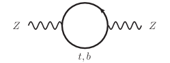
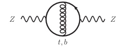
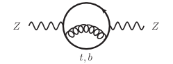
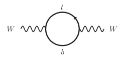
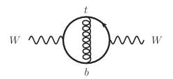
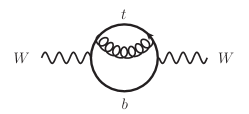
Figure 2: Heavy-quark corrections to the $W$ and $Z$ propagator contributing at $\mathcal{O}\left(G_{F}\right)$ and $\mathcal{O}\left(G_{F}\alpha_{S}\right)$.

As another physical application we calculate the $\rho$ parameter [32] to $\mathcal{O}\left(G_{F}\alpha_{S}\right)$ in FDR. Its deviation from unity $\delta\rho$, defined by

$$\rho=\frac{M_{W}^{2}}{\cos\theta_{w}^{2}M_{Z}^{2}}=1+\delta\rho,$$ (36)

can be expressed in terms of the transverse parts of the weak gauge boson polarization functions $\Pi_{VV}$, $V\in\{W,Z\}$, at zero momentum:

$$\delta\rho=\frac{\Pi_{ZZ}(0)}{M_{Z}^{2}}-\frac{\Pi_{WW}(0)}{M_{W}^{2}}$$ (37)

Typical diagrams contributing up to $\mathcal{O}\left(G_{F}\alpha_{S}\right)$ are shown in Fig. 2.

The DR result [33] depends on the renormalization scheme for $M_{t}$ and reads in the $\overline{\text{MS}}$ and in the on-shell scheme

$$\delta\rho^{\overline{\text{MS}}} =\frac{3G_{F}\left(M_{t}^{\overline{\text{MS}}}\right)^{2}}{8\sqrt{2}\pi^{2}}\left[1+\frac{\alpha_{S}}{\pi}\left(2-\frac{4}{3}\zeta_{2}+2L\right)+\mathcal{O}\left(\alpha_{S}^{2}\right)\right]\;\text{and}$$ (38a)

$$\delta\rho^{\text{pole}} =\frac{3G_{F}\left(M_{t}^{\text{pole}}\right)^{2}}{8\sqrt{2}\pi^{2}}\left[1+\frac{\alpha_{S}}{\pi}\left(-\frac{2}{3}-\frac{4}{3}\zeta_{2}\right)+\mathcal{O}\left(\alpha_{S}^{2}\right)\right],$$ (38b)

respectively, where $L=\ln\left(\frac{\mu^{2}}{M_{t}^{2}}\right)$.

With our numerical FDR setup we obtain at first

$$\delta\rho^{\text{FDR}} =\frac{3G_{F}\left(M_{t}^{\text{FDR}}\right)^{2}}{8\sqrt{2}\pi^{2}}\left[1+\frac{\alpha_{S}}{\pi}\left(2L+0.4734216(3)\right)\right]$$

$$=\frac{3G_{F}\left(M_{t}^{\text{FDR}}\right)^{2}}{8\sqrt{2}\pi^{2}}\left[1+\frac{\alpha_{S}}{\pi}\left(2L+\frac{8}{3}-\frac{4}{3}\zeta_{2}+(4\pm 3)\cdot 10^{-7}\right)\right],$$ (39)

where the top-quark mass is interpreted to be in the FDR scheme, which is related to other schemes via a finite renormalization [2, 5]:

$$\frac{M_{t}^{\text{FDR}}}{M_{t}^{\overline{\text{MS}}}} =\frac{Z_{m}^{\text{FDR}}}{Z_{m}^{\text{$\overline{\text{MS}}$}}}=1-\frac{\alpha_{S}}{3\pi}+\mathcal{O}\left(\alpha_{S}^{2}\right),$$ (40a)

$$\frac{M_{t}^{\text{FDR}}}{M_{t}^{\text{pole}}} =1+\frac{\alpha_{S}}{\pi}\left(-L-\frac{5}{3}\right)+\mathcal{O}\left(\alpha_{S}^{2}\right)$$ (40b)

Inserting either of these relations into Eq. (39) we find agreement with Eq. (38) up to the level of $10^{-7}$.

4 Conclusions

In this paper we have proposed a method to evaluate IR-finite FDR integrals numerically up to two-loop order based on the subtraction of auxiliary integrals, which are constructed by linearizing parts of the denominator in the Feynman parameter representation. The method has been applied successfully to two-loop problems with vanishing external momenta, adding the decay of a pseudoscalar Higgs boson into two photons in the heavy-top limit as well as QCD corrections to the $\rho$ parameter to the list of observables recalculated in FDR. As expected, the treatment of $\gamma_{5}$ was found to be unproblematic in FDR, at least for these examples.

The application to problems with finite external momenta, which is left for future investigations, poses several challenges. Unfortunately, the relations (4) lead to a large number of tensor integrals in the presence of external momenta. Thus it is essential to reduce the number of integrals as much as possible, which could be achieved by the application of integration-by-parts methods [34, 35] as proposed in Ref. [36]. Furthermore, the introduction of additional massless propagators may increase the number of pseudo-thresholds with presumably disadvantageous effects on the stability of the numerical integration.

Acknowledgments.

I would like to thank Robert Harlander for numerous fruitful discussions throughout this project. The Feynman diagrams presented in this paper were created with the help of jaxodraw [37, 38, 39].

References

- [1] R. Pittau, A Four-Dimensional Approach to Quantum Field Theories, JHEP 1211 (2012) 151, [1208.5457].
- [2] A. M. Donati and R. Pittau, FDR, an Easier Way to NNLO Calculations: A Two-Loop Case Study, Eur. Phys. J. C74 (2014) 2864, [1311.3551].
- [3] G. ’t Hooft and M. J. G. Veltman, Regularization and Renormalization of Gauge Fields, Nucl. Phys. B44 (1972) 189–213.
- [4] R. Pittau, QCD Corrections to in FDR, Eur. Phys. J. C74 (2014) 2686, [1307.0705].
- [5] B. Page and R. Pittau, Two-loop off-shell QCD amplitudes in FDR, JHEP 11 (2015) 183, [1506.09093].
- [6] A. Dedes and K. Suxho, Anatomy of the Higgs boson decay into two photons in the unitary gauge, Adv. High Energy Phys. 2013 (2013) 631841, [1210.0141].
- [7] A. M. Donati and R. Pittau, Gauge Invariance at Work in FDR: , JHEP 1304 (2013) 167, [1302.5668].
- [8] A. M. Donati and R. Pittau, The decay of the Higgs boson in FDR, EPJ Web Conf. 60 (2013) 12014, [1306.6785].
- [9] Z. Nagy and D. E. Soper, General subtraction method for numerical calculation of one loop QCD matrix elements, JHEP 09 (2003) 055, [hep-ph/0308127].
- [10] T. Binoth and G. Heinrich, An automatized algorithm to compute infrared divergent multiloop integrals, Nucl. Phys. B585 (2000) 741–759, [hep-ph/0004013].
- [11] G. Heinrich, Sector Decomposition, Int. J. Mod. Phys. A23 (2008) 1457–1486, [0803.4177].
- [12] T. J. E. Zirke, Perturbative Calculations and Their Application to Higgs Physics. PhD thesis, University of Wuppertal, 2014.
- [13] V. A. Smirnov, Feynman Integral Calculus. Springer, 2006.
- [14] D. E. Soper, Techniques for QCD calculations by numerical integration, Phys. Rev. D62 (2000) 014009, [hep-ph/9910292].
- [15] Z. Nagy and D. E. Soper, Numerical Integration of One-Loop Feynman Diagrams for -Photon Amplitudes, Phys. Rev. D74 (2006) 093006, [hep-ph/0610028].
- [16] P. Nogueira, Automatic Feynman Graph Generation, J. Comput. Phys. 105 (1993) 279–289.
- [17] R. Harlander, T. Seidensticker and M. Steinhauser, Complete Corrections of to the Decay of the Boson into Bottom Quarks, Phys. Lett. B426 (1998) 125–132, [hep-ph/9712228].
- [18] T. Seidensticker, Automatic Application of Successive Asymptotic Expansions of Feynman Diagrams, hep-ph/9905298.
- [19] V. A. Smirnov, Applied Asymptotic Expansions in Momenta and Masses, Springer Tracts Mod. Phys. 177 (2002) 1–262.
- [20] V. A. Smirnov, Asymptotic Expansions in Momenta and Masses and Calculation of Feynman Diagrams, Mod. Phys. Lett. A10 (1995) 1485–1500, [hep-th/9412063].
- [21] M. Steinhauser, MATAD: A Program Package for the Computation of Massive Tadpoles, Comput. Phys. Commun. 134 (2001) 335–364, [hep-ph/0009029].
- [22] J. Vermaseren, New Features of FORM, math-ph/0010025.
- [23] M. Tentyukov and J. A. M. Vermaseren, The Multithreaded version of FORM, Comput. Phys. Commun. 181 (2010) 1419–1427, [hep-ph/0702279].
- [24] J. Kuipers, T. Ueda, J. A. M. Vermaseren and J. Vollinga, FORM version 4.0, Comput. Phys. Commun. 184 (2013) 1453–1467, [1203.6543].
- [25] T. Hahn, CUBA: A Library for Multidimensional Numerical Integration, Comput. Phys. Commun. 168 (2005) 78–95, [hep-ph/0404043].
- [26] J. Berntsen, T. O. Espelid and A. Genz, An adaptive algorithm for the approximate calculation of multiple integrals, ACM Trans. Math. Software 17 (1991) 437–451.
- [27] A. Djouadi, M. Spira, J. J. van der Bij and P. M. Zerwas, QCD Corrections to Decays of Higgs Particles in the Intermediate Mass Range, Phys. Lett. B257 (1991) 187–190.
- [28] S. Dawson and R. P. Kauffman, QCD corrections to , Phys. Rev. D47 (1993) 1264–1267.
- [29] S. L. Adler and W. A. Bardeen, Absence of higher order corrections in the anomalous axial vector divergence equation, Phys. Rev. 182 (1969) 1517–1536.
- [30] A. Djouadi, M. Spira and P. M. Zerwas, Two Photon Decay Widths of Higgs Particles, Phys. Lett. B311 (1993) 255–260, [hep-ph/9305335].
- [31] S. A. Larin, The Renormalization of the Axial Anomaly in Dimensional Regularization, Phys. Lett. B303 (1993) 113–118, [hep-ph/9302240].
- [32] D. A. Ross and M. J. G. Veltman, Neutral Currents in Neutrino Experiments, Nucl. Phys. B95 (1975) 135.
- [33] K. G. Chetyrkin, J. H. Kühn and M. Steinhauser, Corrections of Order to the Parameter, Phys. Lett. B351 (1995) 331–338, [hep-ph/9502291].
- [34] F. V. Tkachov, A Theorem on Analytical Calculability of Four Loop Renormalization Group Functions, Phys. Lett. B100 (1981) 65–68.
- [35] K. G. Chetyrkin and F. V. Tkachov, Integration by Parts: The Algorithm to Calculate beta Functions in 4 Loops, Nucl. Phys. B192 (1981) 159–204.
- [36] R. Pittau, Integration-by-parts identities in FDR, Fortsch. Phys. 63 (2015) 601–608, [1408.5345].
- [37] J. A. M. Vermaseren, Axodraw, Comput. Phys. Commun. 83 (1994) 45–58.
- [38] D. Binosi and L. Theussl, JaxoDraw: A Graphical user interface for drawing Feynman diagrams, Comput. Phys. Commun. 161 (2004) 76–86, [hep-ph/0309015].
- [39] D. Binosi, J. Collins, C. Kaufhold and L. Theussl, JaxoDraw: A Graphical user interface for drawing Feynman diagrams. Version 2.0 release notes, Comput. Phys. Commun. 180 (2009) 1709–1715, [0811.4113].